Spectro-Imaging Forward Model of Red and Blue Galaxies

Abstract

For the next generation of spectroscopic galaxy surveys, it is important to forecast their performances and to accurately interpret their large data sets. For this purpose, it is necessary to consistently simulate different populations of galaxies, in particular Emission Line Galaxies (ELGs), less used in the past for cosmological purposes. In this work, we further the forward modeling approach presented in Fagioli et al. 2018, by extending the spectra simulator Uspec to model galaxies of different kinds with improved parameters from Tortorelli et al. 2020. Furthermore, we improve the modeling of the selection function by using the image simulator Ufig. We apply this to the Sloan Digital Sky Survey (SDSS), and simulate $\sim 157,000$ multi-band images. We pre-process and analyse them to apply cuts for target selection, and finally simulate SDSS/BOSS DR14 galaxy spectra. We compute photometric, astrometric and spectroscopic properties for red and blue, real and simulated galaxies, finding very good agreement. We compare the statistical properties of the samples by decomposing them with Principal Component Analysis (PCA). We find very good agreement for red galaxies and a good, but less pronounced one, for blue galaxies, as expected given the known difficulty of simulating those. Finally, we derive stellar population properties, mass-to-light ratios, ages and metallicities, for all samples, finding again very good agreement. This shows how this method can be used not only to forecast cosmology surveys, but it is also able to provide insights into studies of galaxy formation and evolution.

1 Introduction

The current and vastly accepted description of the evolution of our Universe includes the idea that it is in a phase of accelerated expansion. A number of observables probe this scenario, including the Hubble parameter $H(z)$ and the angular diameter distance $D_{A}(z)$. These probes are linked to the (baryonic and not) matter content and properties of our Universe [1, 2].

Any dynamical study, including that of the Universe as a whole, requires a working definition of a distance scale. What is used in cosmology are the so called standard rulers [3], whose evolution with cosmic time and size are known. A very good candidate for that are the Baryon Acoustic Oscillations (BAOs) [2]. BAOs encode the width of primordial density fluctuations, which have been propagating in the form of acoustic waves. With the help of General Relativity, these can be expressed in the form of $H(z)$ and $D_{A}(z)$. Also, because of hydrodynamics, BAOs result in over-densities of baryons in shells at the sound horizon scale around an initial baryon over-density. These over-densities are the locations where galaxies formed, inside dark matter halos, through gravitational collapse [4, 5, 6].

This is the reason why understanding how galaxies are located in the Universe is of fundamental importance. In particular, galaxy 3D distribution needs to be explored. While figuring out the celestial coordinates of an object is nowadays not especially challenging, understanding how far an object is from us, or, in other words, its redshift $z$, is not straightforward. Multi-band imaging can be used to estimate photometric redshifts, which however require precise calibration and may suffer from catastrophic outliers. The precise distance of an object from us can be accurately estimated by looking at how much the features on its spectrum are displaced with respect to their laboratory wavelength value. This is a measure of its spectroscopic redshift $z$. In order to do so on a large scale, spectroscopic redshift surveys are required.

In the last decades, cosmology oriented surveys have collected data mainly on the population of the so-called Luminous Red Galaxies (LRGs) [7], see for example the Deep Extragalactic Evolutionary Probe (DEEP2) [8], the Very Large Telescope Deep Survey (VVDS) [9] and the Baryon Oscillation Spectroscopic Survey (BOSS) [10] within the Sloan Digital Sky Survey (SDSS) III [11]. However, the newer-generation spectroscopic surveys like extended-BOSS (eBOSS), [12], the Dark Energy Spectroscopic Instrument (DESI) [13], the 4m Multi-Object Spectroscopic Telescope (4MOST) [14] and Subaru-Prime Focus Spectrograph (PFS) [15] aim at collecting data of a larger volume, up to the $z\sim 2$ population of Emission Lines, or blue, Galaxies (ELGs). These were precedently almost unexplored in cosmological studies due to technical limitations [16, 17], as ELGs are faint targets with emission features lying in the near-infrared background-dominated region of the spectrum at those redshifts. The combination of the two samples of ELGs and LRGs, probing different regions and cosmic times, will provide the most complete 3D map of the Universe to date.

To forecast and properly analyze these future experiments, it is therefore necessary to be able to properly simulate a wider variety of galaxies than the in past. Also, to appropriately account for possible observational biases, the simulation of a spectroscopic survey must be preceded by that of its parent imaging survey, the survey used to select targets for spectroscopy. As spectroscopic surveys require long integration time, it is crucial to appropriately pre-select suitable targets. Reproducing this step avoids that differences in the comparison between data and simulations may be originated from, for example, different magnitude definitions or star-galaxy separations, rather than the simulation itself. Also, computing speed is essential to simulate large amount of data, which is why we present here several software tools which have been developed in order to achieve this.

In this work, we aim at forward modeling a wide field imaging survey such that SDSS, and, consequently, its spectroscopic counterpart. The main idea of forward modeling [18, 19, 20] is to combine an (simple yet realistic) astrophysical model, e.g., the evolution of the luminosity functions of red and blue galaxies with cosmic time, with instrumental parameters, in order to generate realistic simulations. The model can be complexified if the need of more detailed physics appears clear. In forward modeling, data and simulations are analyzed in the same way and compared. The inputs of the simulations can be adjusted such that their agreement improves. This has been proven to be successful for wide-field imaging surveys [20, 19], a narrow-band imaging survey like PAUs (Physics of the Accelerating Universe Survey) [21], and a spectroscopic survey like SDSS [22], hereafter [F18]. After simulating SDSS imaging data, we performe cuts on both data and simulations to obtain suitable samples for red and blue (or bluer, as stated in the CMASS Sparse definition) galaxies. We then forward model SDSS spectra, and compare those to data.

It is important to note that successfully simulating galaxy spectra with this technique means also having a successful galaxy model as a starting point. Also, it means being able to recover basic galaxy properties, such that this method can be also useful in galaxy formation and evolution studies. In the course of this paper, we will show that these two goals have been fulfilled. The galaxy population model, consisting in two different redshift-dependent luminosity functions for red and blue galaxies, has been presented in [19], and fully updated in [23], by using wide-field CFHTLS imaging data [24]. The model parameters derived in [23] are those used to simulate images and spectra in this work. Its successful application to independent spectroscopic data is a further proof of the validity of the method.

The interpretation of absorption (and emission) features tells us about the origin and evolution of galaxies, of their stellar and gas components [25, 26, 27, 28, 29, 30, 31, 32, 33, 34, 31, 35, 36, 37, 38]. This is of fundamental importance for the field of galaxy evolution. In this work, we recovered basic stellar population properties (mass to light ratios, stellar ages, and stellar metallicities) through full spectral fitting [39, 40, 41, 42] for simulated spectra and compared those to real data, finding very good agreement, proving the usefulness of this method for measuring a broad range of galaxy properties.

This paper is constructed as follows. As in forward modeling a combination of input galaxy model and instrumental parameters is used, we review in Section 2 the galaxy population model, from its foundations to its most recent update obtained through an Approximate Bayesian Computation (ABC) run. This final, updated model is what we used throughout the rest of this work. Then, in Section 3, we describe our sample data, needed for both the imaging and the spectroscopic analysis of this work. In Section 4, we describe our image and spectra simulations, respectively performed with the Ultra Fast Image Generator (Ufig) [43], and Uspec [F18]. In Section 5, we describe our analysis pipeline to obtain both photometric and spectroscopic measurements. In Section 6, we comment on our findings and in Section 8 we present our conclusions.

Throughout this work, we use a standard $\Lambda$CDM cosmology with $\Omega_{\mathrm{m}}=0.3$, $\Omega_{\Lambda}=0.7$ and $\mathrm{H}_{0}=70$ km $\mathrm{s}^{-1}\,\mathrm{Mpc}^{-1}$.

2 Galaxy Population Model

2.1 Model Description

Galaxy spectra encode unique information about galaxy (light emitting) content, i.e., stars and gas. To better understand such information, we need to simulate realistic galaxy spectra. The underlying idea is to start from basic galaxy properties, which are used as inputs in the simulations, that together with instrumental parameters produce realistic simulated data, which can be images, or spectra. The model can be complexified to match observations, as outlined in Section 2.2. The model from which such properties are drawn is fully described in [19], and the model parameter values have been further updated in [23], as described in Section 2.2. We here describe the main ideas behind this model.

Galaxy redshifts and magnitudes (and spectral coefficients, as further described below) are drawn from galaxy luminosity functions $\phi$ (see e.g. [44, 45]). The galaxy luminosity function describes the number of galaxies $N$ per comoving volume $V$ in Mpc and absolute magnitude $M$:

$$\phi(z,M)=\frac{dN}{dM\,dV}$$ (2.1)

where $z$ denotes redshift. Galaxies are drawn from separate and redshift dependent luminosity functions for blue and red objects. The redshifts and absolute magnitudes are obtained by sampling from the corresponding luminosity function. Then Spectral Energy Distributions (SEDs) are modeled. SEDs of galaxies are defined as linear combinations of templates $T_{i}(\lambda)$ and coefficients $c_{i}$, where $T_{i}(\lambda)$ are the templates and $c_{i}$ come from a Dirichlet distribution [46] of order five, as described in [19]. This model made use of the NYU Value-Added Galaxy Catalog (NYU-VAGC) [47], using as templates the $kcorrect$ templates presented in [48]. These are based on Bruzual $\&$ Charlot stellar templates [49]. The stellar templates span an age range from 1 Myr to 13.75 Gyrs, and total stellar metallicities of $Z=0.0001,0.0004,0.004,0.008,0.02$ and $0.05$, where $Z=0.02$ is the value for solar metallicity. The templates have solar $\alpha$-to-iron ($[\alpha/$Fe]) ratios. 35 templates come from MAPPINGS-III [50] models of emission from ionized gas, which is what allows us to simulate bluer galaxies with emission features. Different coefficients $c_{i}$ are used for blue and red galaxies, coming from different Dirinchlet distributions, and they are redshift evolving, as better described below. The coefficients $c_{i}$ and redshifts $z$ are then given as inputs for the spectra simulations. The luminosity function parameters and magnitudes are used to render galaxy images.

2.2 Model calibration through Approximate Bayesian Computation

		Blue	Red
Luminosity Function Parameters	$\alpha$	-1.3	-0.5
	$\mathrm{M^{*}_{B,slope}}$	-0.417	-0.610
	$\mathrm{M^{*}_{B,intcpt}}-5\log{h_{70}}$	-20.591	-20.416
	$\mathrm{\phi^{*}_{amp}}$ / 10-3 h${}^{3}_{70}$ Mpc-3 mag-1	0.0063	0.0141
	$\mathrm{\phi^{*}_{exp}}$	-0.264	-2.232
Size Parameters	$\mathrm{r_{50,slope}^{phys}}$	-0.243	-0.243
	$\mathrm{r_{50,intcpt}^{phys}}$	0.954	0.954
	$\mathrm{\sigma_{phys}}$	0.568	0.568
Spectral Coefficients	$\mathrm{a}_{1,0}$	2.079	2.461
	$\mathrm{a}_{2,0}$	3.524	2.358
	$\mathrm{a}_{3,0}$	1.917	2.568
	$\mathrm{a}_{4,0}$	1.992	2.268
	$\mathrm{a}_{5,0}$	2.536	2.402
	$\mathrm{a}_{1,1}$	2.265	2.410
	$\mathrm{a}_{2,1}$	3.862	2.340
	$\mathrm{a}_{3,1}$	1.921	2.200
	$\mathrm{a}_{4,1}$	1.685	2.540
	$\mathrm{a}_{5,1}$	2.480	2.464

Table 1: Median values of the galaxy model parameters for red and blue galaxies. In this table, the first 5 entries are the numerical values for the luminosity function parameters of Equation 2.2. $\mathrm{r_{50,slope}^{phys}}$, $\mathrm{r_{50,intcpt}^{phys}}$ and $\mathrm{\sigma_{phys}}$ are size parameters also derived in [23]. The spectral coefficients are $\mathrm{a}_{\mathrm{i},0}$, which describe the galaxy population at $z=0$, and $\mathrm{a}_{\mathrm{i},1}$, at redshift $z=z_{1}>0$. The spectral coefficients come from a Dirichlet distribution of order $5$.

The galaxy population model described above is calibrated in [23]. In that work, we use Approximate Bayesian Computation (ABC) [51] to constrain the galaxy population model parameters by matching simulations and data in an iterative way. ABC is a technique to approximate a Bayesian posterior by restricting the prior space in an iterative way, for cases where no clear likelihood can be provided. The prior space is reduced by minimising one or more distance metrics, which are described in details in [23]. The data used in that work are images coming from Canada-France-Hawaii Telescope Legacy Survey (CFHTLS) wide-field galaxy survey [24]. Image simulations are performed with Ufig. As explained above, the aim of that work is to calibrate the galaxy population model and consequently measure the luminosity function of red and blue galaxies.

The luminosity functions of red and blue galaxies can be expressed as

$$\Phi(\mathrm{M,z})\mathrm{dM}\,=\,\frac{2}{5}\ln{(10)}\phi^{*}(z)10^{\frac{2}{5}(\mathrm{M^{*}(z)-M})(\alpha(z)+1)}\mathrm{e}^{\left[-10^{\frac{2}{5}(\mathrm{M(z)^{*}-M})}\right]}\mathrm{dM}$$ (2.2)

where M is the absolute magnitude of a galaxy, $z$ its redshift, $\phi*$ the normalization of the Schechter function [52], M^∗ defines where the luminosity function transitions from a power law to a decaying exponential function, and $\alpha$ sets the faint end slope. The model parameters obtained with this run are listed in Table 1, together with spectral coefficients and size parameters. The spectral coefficients evolve as

$$\mathrm{a_{i}\left(z\right)=\left(a_{i,0}\right)^{1-z/z_{1}}\times\left(a_{i,1}\right)^{z/z_{1}}}$$ (2.3)

where $\mathrm{a}_{\mathrm{i},0}$ describes the galaxy population at $z=0$, while $\mathrm{a}_{\mathrm{i},1}$ at redshift $z=z_{1}>0$. The spectral coefficients come from a Dirichlet distribution of order $5$ and their values, which can be also found in Table 1, are used to generate spectra in this work.

3 Data

3.1 Images

3.1.1 Image Retrieval

We use data from SDSS (Sloan Digital Sky Survey) DR14 (server path: http://dr12.sdss.org/sas/dr14/eboss/photoObj/frames/301/). Images and spectra were obtained at the 2.5m telescope of the Apache Point Observatory (APO) in Sunspot, New Mexico [53]. Each SDSS image can be uniquely identified by a sequence of three number, namely run, camera column (or "camcol"), and field. All information about SDSS imaging data can be found at http://www.sdss3.org/dr10/imaging/imaging_basics.php. We randomly select camcol, field and run to construct the path to the images. We download 157,000 images, all of them in five bands (ugriz). Alongside with each image, we download a star catalog from GAIA DR2 [54, 55] through the VizieR database of astronomical catalogues [56], within a radius of $0.3$ degrees around the central pixel coordinates in each field. The use of this star catalog is explained in Section 3.1.2.

3.1.2 Image Processing

In order for the images to be usable for forced photometry and spectra retrieval, some steps are necessary to pre-process them. Also, we need to compute some instrument-specific parameters to be able to properly simulate SDSS-like images. In the following paragraphs, we explain this procedure in details.

Alignment

SDSS images are downloaded in 5 bands ($ugriz$). The same field in different bands shows a dithering of $\sim 5-15$ pixels. This makes the computation of magnitudes with SExtractor forced photometry incorrect. Forced photometry uses a reference image for the source coordinates, and then draws apertures and computes fluxes according to this reference. Therefore, a misalignment would result in a wrong magnitude computation.

To align the field with pixel precision in the different bands we use SWarp [57]. SWarp is a C-based software that resamples and co-adds together FITS images using an astrometric projection chosen by the user among a list in the World Coordinate System (WCS) standards. We use the standard param.swarp given configuration file, except for those keywords which are survey specific.

Astrometry

The alignment of SDSS images in five different bands using SWarp introduces an error in their astrometry. To fix this issue, we run SCAMP [58]. SCAMP reads SExtractor [59] catalogs and computes astrometric and photometric solutions for any arbitrary sequence of FITS images. For this purpose, we first run SExtractor with SCAMP specific parameters. SCAMP computes the astrometric solution by using as a reference the GAIA catalog described in 3.1.1. Then we update the FITS headers of SDSS images with the new computed WCS specific keywords.

Simulation Parameters Estimation

• PSF: As described in Section 3.1.1, each set of images in the five $ugriz$ bands has an associated star catalog coming from GAIA. We use the star catalog to estimate the seeing and beta ($\beta$) values of the circular Moffat function, which is assumed to describe the star 1D light profile in SDSS [60]. We match the GAIA catalog to each image to securely identify stars. We then select stars within the magnitude range $14<\mathrm{mag\,g}<16$, to avoid faint or saturated stars. We make cutouts around the matched stars in the SDSS images. We then fit a two-dimentional Moffat profile, and consider the fitted median Full Width Half Maximum (FWHM) and $\beta$ as the input values for our Ufig simulations.

• Background: The background is directly estimated from SDSS images. We first run SExtractor to obtain a segmentation image, i.e., an image that separates objects from the sky background. Taking values coming only from regions identified as sky background, we compute the mean $\mu$ and the standard deviation $\sigma$, applying a 4$\sigma$ clipping. We then use those as parameters to simulate the gaussian sky background in Ufig.

• Magnitude Zeropoint: The magnitude zeropoint in SDSS is computed as $-2.5\,\log_{10}f$, where $f$ is the flux expressed in maggies (1 maggie is the flux density in Janskys divided by 3631). The $f$ value in nanomaggies ($10^{-9}$ maggies) is contained in the keyword ‘NMGY’ in the header of the SDSS fits images. It has been found that the $u-$band value needs to be shifted by $0.04$ mag in order to match the standard AB magnitude system [61], which we do in our simulations.

• Pixel Scale: The pixel scale for SDSS images is $0.396\operatorname{arcsec}$/pixel.

• Gain: Gain values in SDSS are specific for each camcol and filter. The full list can be found at https://data.sdss.org/datamodel/files/BOSS_PHOTOOBJ/frames/RERUN/RUN/CAMCOL/frame.html.

• Saturation: The imaging data saturate at about 13, 14, 14, 14, 12 magnitudes for point sources.

• Exposure time and filters: The five filters are observed in order r i u z g, 71.7 seconds apart. The integration time in each filter is $\sim 54$ seconds.

3.2 Spectra

Spectra are downloaded through the astroquery package [62], from SDSS DR14 spectroscopic data release. We use the RA and DEC coordinates stored in the SExtractor variables (ALPHAWIN_J2000 and DELTAWIN_J2000) and query spectra within $1\operatorname{arcsec}$ searching radius. We only download spectra observed with the BOSS (Baryon Oscillation Spectroscopic Survey) instrument [10, 11], and with $z>0$, so to avoid negative or nan values.

4 Simulations

4.1 Image Simulation

We simulate SDSS imaging data with the Ultra Fast Image Generator (Ufig) [43, 63, 64, 65, 19, 20, 21, 66, 23]. Ufig simulates astronomical images by combining parameters coming from a galaxy population model (magnitudes, sizes and Sérsic profiles) as described in Section 2, and instrumental parameters coming from the survey we aim at simulating. Ufig ability of simulating a variety of wide- (DES, COSMOS, CFHTLS) and narrow- (PAUS) band survey has been shown in [43, 63, 64, 65, 19, 20, 21, 66, 23]. This is the first time Ufig is used to render SDSS images. We use the instrumental properties derived as described in Section 3.1.2. Figure 1 shows the comparison between a real image from SDSS (left hand side) and a Ufig simulated image (right hand side). We run tests to assess the reliability of our image simulation, comparing the pixel and number counts for real and simulated images [43], finding very good agreement. For further details on Ufig and particularly on its speed, we refer the reader to [43].

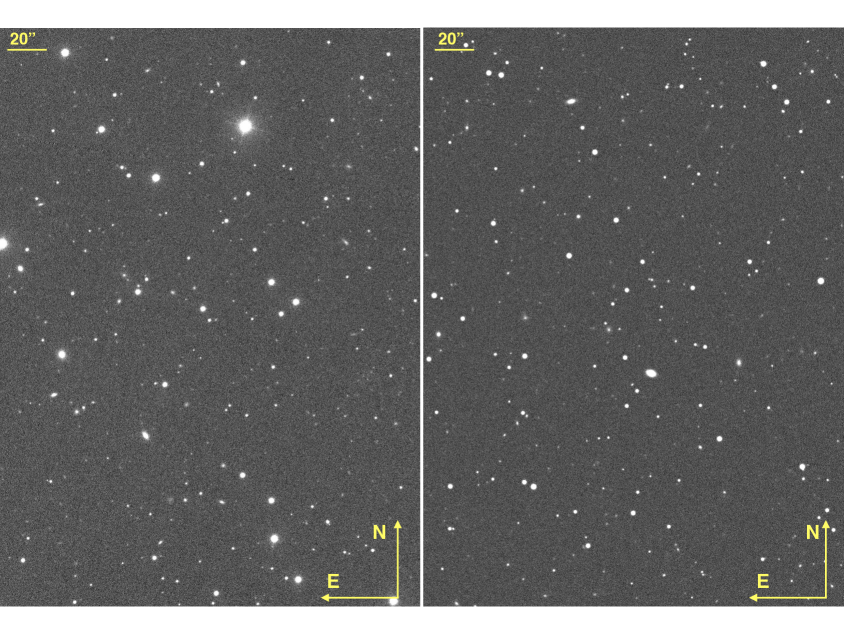
Figure 1: Comparison between a SDSS real (left panel) and simulated (right panel) $i-$band image. The real SDSS image has been preprocessed as described in Section 3. The north and east directions are shown at the bottom of the panels with yellow arrows. The upper left thick shows the angular size on the image corresponding to $20\operatorname{arcsec}$.

4.2 Spectra Simulation

We simulate galaxy spectra with our software Uspec. Uspec has been presented and described in details in [F18]. Uspec usage is fully outlined in the flowchart in Figure 3 in [F18]. Briefly, Uspec takes as inputs the galaxy model described in Section 2, and also in [19] and [23], and the instrumental setup (read-out noise, shot noise, transmission curve, exposure time) of a given telescope. As an update from the previous version of Uspec, we now include the effects of Galactic dust, following the extinction curve for diffuse gas from [67] with $R_{v}=3.1$, and using the Galactic $E(B-V)$ values from the maps of [68], in our spectra simulations. It is important to mention that one of the main noise contaminants in galaxy spectra is the spectrum coming from our own atmosphere. In [F18], we explain in details how we account for this effect, and in Figure 4 of [F18] we show the sky model which is also used in this work, and how we constructed it. In the end, Uspec outputs redshifted, noisy galaxy spectra, for both blue and red galaxies. This differentiation derives from the different spectral coefficients coming by different luminosity functions for red and blue galaxies, drawn together with magnitudes and redshifts. These spectral coefficients are combined with $kcorrect$ spectral templates [48] to produce galaxy model spectra.

5 Analysis

5.1 Imaging Measurements

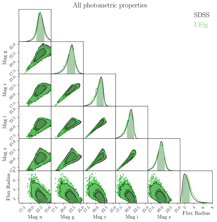
Figure 2: Comparison of galaxy imaging properties between real (black) and simulated (green) data. The 5 ($ugriz$) SDSS band are shown, together with the SExtractor FLUX_RADIUS parameter. The magnitude distributions are the $\mathrm{mag}_{\mathrm{corr}}$ defined in Equation 5.1 in Section 5.1. The agreement between data and simulation is particularly noteworthy as in no stage of the galaxy model parameters calibration in [23] SDSS images have been used.

The large amount of data, and, accordingly, simulations, required for this work, made the use of the multiple cores of the Euler cluster necessary. The whole analysis and simulations described above take about 4 hours with 1,000 cores.

We perform imaging measurements on both simulated and real images with SExtractor. On each pair of real and simulated SDSS fields (the real field from SDSS and its analog, i.e., a simulated image with instrumental parameters measured as described in Section 3.1.2), we run SExtractor in forced photometry mode in the five $ugriz$ bands. In order to do so, we construct a detection image as described in [69] and summarized in [23], and references therein. In brief, we stack the $ugriz$ images and normalize each of them by their background $\sigma$ computed as described in 3.1.2. We then used the maximum seeing, magnitude zeropoint, saturation and gain within the five images. The use of the maximum seeing ensures we do not loose signal coming from the source. This is further guaranteed by the alignment of the images made through SWarp. We then measure magnitudes in each band by using the aperture fixed in the detection image, and correct those for the different PSF among bands as described in [69] and as shown below:

$$\begin{array}[]{l}u_{\mathrm{corr}}=u_{\mathrm{ISO}}-(d_{\mathrm{ISO}}-d_{\mathrm{AUTO}})\\ g_{\mathrm{corr}}=g_{\mathrm{ISO}}-(d_{\mathrm{ISO}}-d_{\mathrm{AUTO}})\\ r_{\mathrm{corr}}=r_{\mathrm{ISO}}-(d_{\mathrm{ISO}}-d_{\mathrm{AUTO}})\\ i_{\mathrm{corr}}=i_{\mathrm{ISO}}-(d_{\mathrm{ISO}}-d_{\mathrm{AUTO}})\\ z_{\mathrm{corr}}=z_{\mathrm{ISO}}-(d_{\mathrm{ISO}}-d_{\mathrm{AUTO}}),\end{array}$$ (5.1)

where $d_{\mathrm{ISO}}$ and $d_{\mathrm{AUTO}}$ are the SExtractor MAG_ISO and MAG_AUTO measured on the detection image. We measure and store also FLUX_RADIUS and coordinates RA and DEC for later usage. The same procedure is applied to data and simulations, as in the philosophy of forward modeling.

Figure 2 shows the agreement between our real (black) and simulated (green) $\mathrm{mag}_{\mathrm{corr}}$ and the SExtractor FLUX_RADIUS parameter. This agreement on SDSS imaging measurements is a further proof of the goodness of the luminosity function parameters computed in [23], as it shows that same parameters can be applied to different surveys than those used in the ABC run. It is noteworthy that in no stage of the ABC run SDSS was used to constrain the luminosity function parameters, and yet here it is shown that SDSS images can be properly simulated with those parameters.

5.2 Selection Cuts

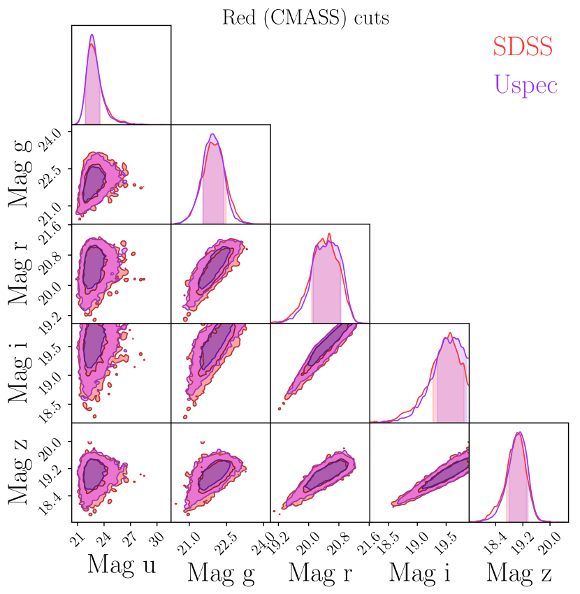
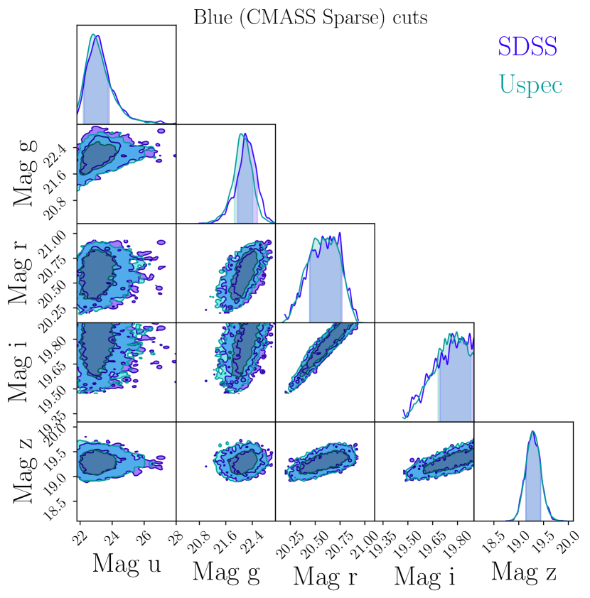
Figure 3: Comparison between photometric properties of real and simulated data for red (left panel) and blue (right panel) galaxies. Both panels show magnitudes of objects after applying the CMASS (for red galaxies) and CMASS Sparse (for blue galaxies) cuts. For all galaxies shown in this panel we retrieved the spectra which are later used in our spectroscopic analysis.

We emulate cuts as in the SDSS/BOSS CMASS sample [70]. For a more extensive description of these cuts, please read [F18], and references therein. We call this sample the red galaxies sample throughout the rest of this paper. In addition, we emulated the CMASS Sparse sample cuts. We call this sample the blue galaxies sample throughout the rest of this paper, as this is defined to be a sample of fainter and bluer galaxies with respect to CMASS. CMASS Sparse has been designed to randomly select 1 in about 10 targets.
Our specific magnitude (i.e., our $\mathrm{mag}_{\mathrm{corr}}$ as described above), color, and star-galaxy separation cuts are listed below:

CMASS, or Red Galaxies

• $17.5<\mathrm{mag}\,i<19.9$

• $r-i<2$

• $d_{\perp}>0.55$, where $d_{\perp}=(r-i)-(g-r)/8$

• $\mathrm{mag}\,i<19.86+1.6\times(d_{\perp}-0.8)$

• SExtractor CLASS_STAR < 0.1, for star-galaxy separation

CMASS Sparse, or Blue Galaxies

• $17.5<\mathrm{mag}\,i<19.9$

• $r-i<2$

• $d_{\perp}>0.55$, where $d_{\perp}=(r-i)-(g-r)/8$

• $\mathrm{mag}\,i<20.14+1.6\times(d_{\perp}-0.8)$

• SExtractor CLASS_STAR < 0.1, for star-galaxy separation

The SExtractor CLASS_STAR < 0.1 has been used to ensure purity of the sample from stars or quasars. However, no appreciable differences can be seen when applying a CLASS_STAR cut of $<0.9$.

Figure 3 shows the comparison between real and simulated magnitudes after applying the above cuts for red and blue galaxies. The two samples show a good agreement overall, with however a small shift towards fainter magnitudes for SDSS in the central $gri$ bands. A similar difference can be seen in Figure 7 in [23]. This is likely to be an observational effect due to BOSS targeting that our forward modeling technique is not able to reproduce at the current stage, as we do not see any sign of this in the magnitude comparison for the whole sample (Figure 2).

Figure 4 shows the color-magnitude comparison between SDSS CMASS and CMASS Sparse. On the left hand panel, a comparison between the $g-i$ color and the magnitude in the $i-$band of SDSS red (CMASS) and SDSS blue (CMASS sparse) samples is shown. The same on the right hand side panel, but for simulations. The two figures show how both data and simulation have the same behaviour, with the CMASS Sparse-like sample occupying the region of fainter magnitudes of the CMASS sample. CMASS Sparse is indeed described as a sample of bluer and fainter galaxies, and this is expressed in the cuts listed in Section 5.2.

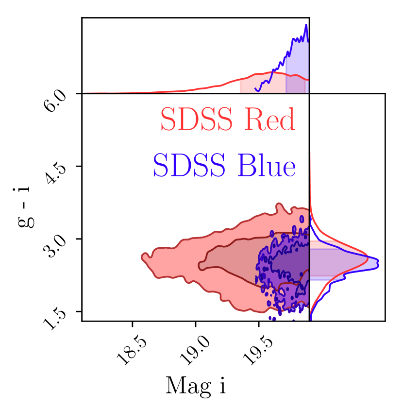
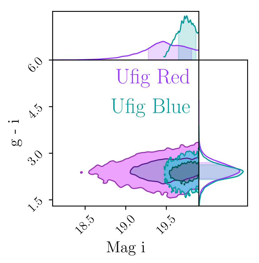
Figure 4: Color (g-i) - magnitude ($i-$band) diagram for real and simulated data. We used the $\mathrm{mag}_{\mathrm{corr}}$ described in Section 5.1. On the left hand side, a comparison between the CMASS (red) and CMASS Sparse (blue) galaxies from the SDSS survey. CMASS Sparse is defined to target bluer and fainter objects than the parent sample CMASS. This is visible also in our contours. The same trends are visible in the simulated samples on the right hand side on the plot.

5.3 Spectroscopic Measurements

After galaxies are selected according to the cuts described above, galaxy spectra for both the blue and the red samples are downloaded, as described in Section 3.2. The spectra are then analysed and compared with two different techniques: by using Principal Components Analysis (PCA), and by looking at their stellar population properties computed with full spectral fitting. The results coming from these two analysis are shown in Figures 5, 6, 7 and 9, and described in details in Section 6. Here we describe the methodologies we use for these two kinds of analysis.

5.3.1 Principal Components Analysis

Our use of PCA in comparing data and simulation has been already described in details in [F18] and [21]. To briefly summarize, applying PCA means in this case representing the spectra as a set of eigenspectra of lower dimension, as also shown in [71]. We use Singular Value Decomposition to compute the eigenspectra and eigencoefficients, as sets of spectra can be described as

$${f}(\lambda)=\sum_{j}\mathrm{a}_{j}\phi_{j}(\lambda)\,~{}~{}\mathrm{for\,data}$$ (5.2)

$${f^{\prime}}(\lambda)=\sum_{j}\mathrm{b}_{j}\psi_{j}(\lambda)\,~{}~{}\mathrm{for\,simulations}$$ (5.3)

where a_j, or b_j, are the eigencoefficients, and $\phi_{j}(\lambda)$, or $\psi_{j}(\lambda)$, are the eigenspectra for the data or the simulations, accordingly.

These are computed independently for data and simulations, and can be compared through the Mixing Matrix. We define the Mixing Matrix as

$$\mathrm{M}_{ij}=\int\phi_{i}(\lambda)\psi_{j}(\lambda)~{}d\lambda$$ (5.4)

so that, if $\phi_{i}(\lambda)\equiv\psi_{i}(\lambda)$, $\mathrm{M}_{ij}$ reduces to

$$\mathrm{M}_{ij}=\delta_{ij}$$ (5.5)

which means that, if real and simulated data were described by the same basis set, the mixing matrix would be the Identity Matrix.

For this analysis, we mask regions where strong sky lines are expected (4403 Å, 5350 Å, 5577 Å, 5588 Å, 5894.6 Å, 6301.7 Å, 6364.5 Å, 7246.0 Å, 7074 Å  with 20 Å  width, the grey stripes in Figures 5 and 6), and we exclude the $10\%$ brightest objects in the two samples, so that the outliers would not dominate the principal components. The data and simulations are analysed with matching their redshift distributions. Further details on this aspect can be found in Section 6.2. This procedure is applied to both data and simulations.

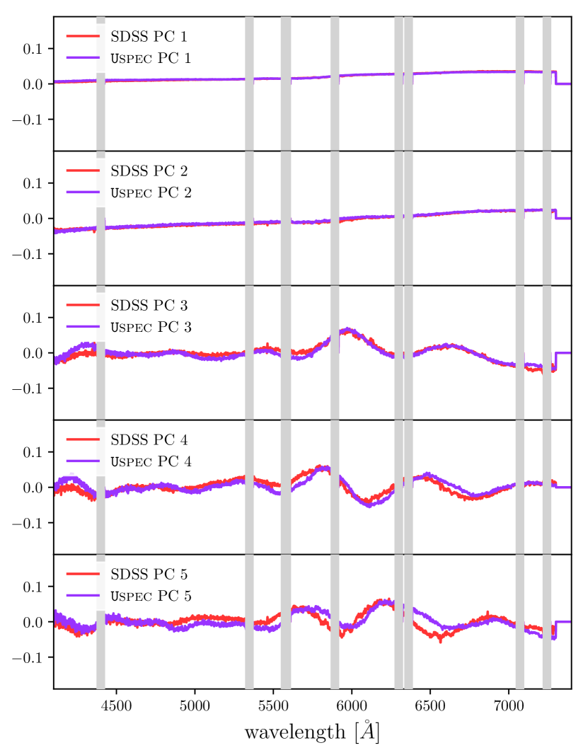
Figure 5: Mixing matrix and first 5 PCA components for red galaxies. The comparison between all first five principal components shows a very good agreement between data and simulations. This is quantified in the Mixing Matrix shown on the left hand side of the plot.

5.3.2 Full Spectral Fitting

We use full spectral fitting to compute stellar population parameters. Full spectral fitting is a technique which has been developed to compute stellar population parameters [39, 40, 41, 42], mostly stellar ages and stellar metallicities, but can also include stellar masses and gas properties. Fitting the whole spectrum at the same time constitutes an advancement on the older technique which consisted in fitting individual absorption features and their pseudo-continua [25, 26, 27, 28, 29, 30, 31, 32, 33, 34, 31, 35, 36, 37, 37, 38]. In this paper, we used the latest version of Penalized Pixel-Fitting (pPXF) [72] to perform full spectral fitting. We use templates from the MILES library [73], with a wide range of stellar ages and metallicities, and solar $[\alpha/$Fe] ratios. During the fit we use a 20th order multiplicative polynomial correction and no additive polynomials, as recommended in [72]. We do not fit the gas component simultaneously, to improve the speed of the fit. We derived stellar ages, metallicities and mass to $r-$band based light ratios as described in detail in Section 6.

6 Results

6.1 Principal Components

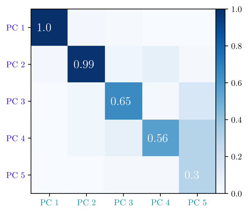
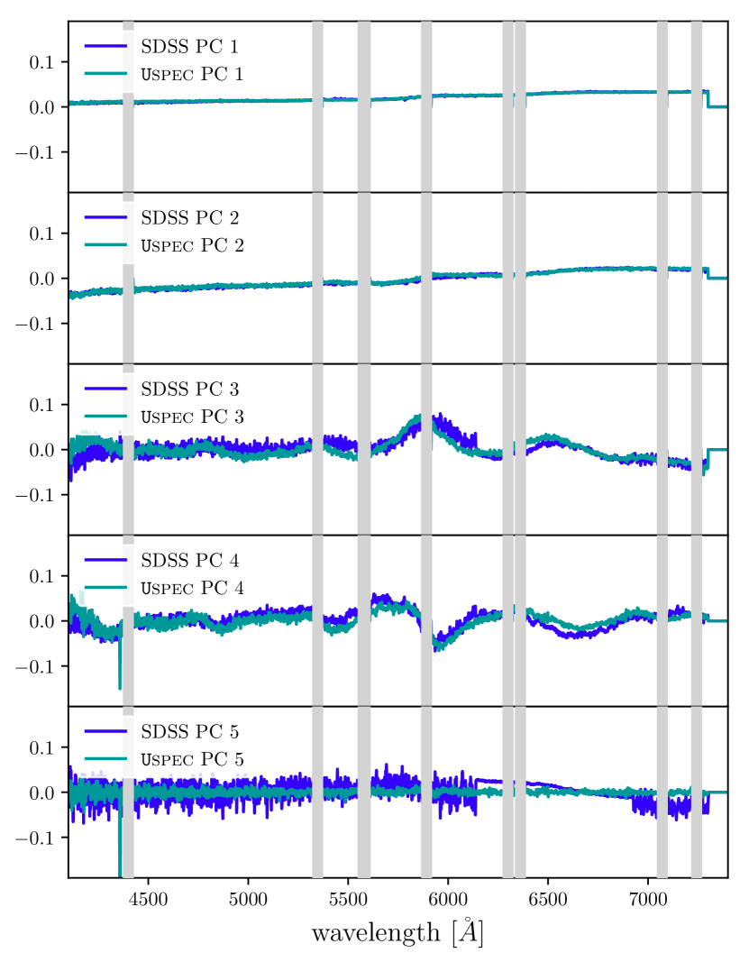
Figure 6: Mixing matrix and first 5 PCA components for blue galaxies. The comparison of the first two principal components shows excellent agreement. A less good agreement is shown for higher order principal components, as expected for blue galaxies, notoriously known as difficult to individually, rather than statistically, simulate. Higher order principal component are more sensitive to individual galaxy features. As in the previous Figure, the comparison between principal components is quantified in the Mixing Matrix shown on the left hand side of the plot.

In order to assess our ability to properly simulate galaxy spectra, we use PCA to quantify the agreement between our spectra simulation and SDSS data. The methodology has been described in details in [F18], and [21], and in Section 5.3.1. The first five eingenspectra, or principal components, we decomposed our galaxies into are shown in Figures 5 (red galaxies) and Figure 6 (blue galaxies), in the right panels. In the left panels, we show the associated Mixing Matrices, as described in Section 5.3.1.

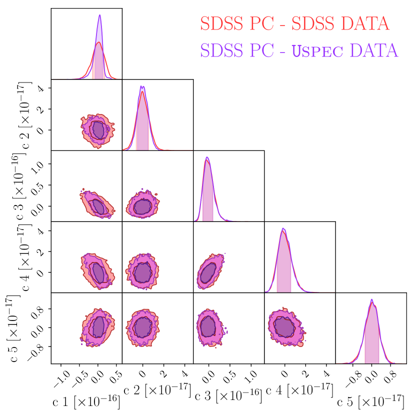
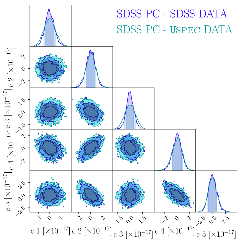
Figure 7: Eigencoefficients resulting from projecting real spectra from SDSS and simulated Uspec spectra onto SDSS principal components. The distributions for all the first five principal components appear to be centered to each other and present the same width, for both red and blue galaxies. The eigencoefficients are expressed in the same units of flux ($10^{-17}\mathrm{ergs}\,s^{-1}\,\textup{\AA}^{-1}\,\mathrm{cm}^{-2}$) as the real and simulated spectra.

As seen in Figure 5, red galaxies principal components show very good agreement. For the first component, which encodes most of the information coming from the galaxy population, we find very good agreement between data and simulations, showing that our galaxy population model, derived in [23] and summarized in Section 2.2, is successful not only in reproducing photometric galaxy properties and redshift distributions for the surveys it has been designed for, but also at reproducing spectroscopic galaxy properties for a completely independent survey as SDSS. This is impressive, as the very good agreement can be seen in both the populations of red and blue galaxies when looking at the first two principal components. Differences arise when looking at the higher order components, mostly in the blue galaxy population. In Figure 5, we see good to medium agreement up to the fifth principal component for the red galaxy sample. Individual features are not clearly visible, as this analysis is conducted in observed-frame. However, redshift distribution broadened absorption lines are visible, such as the G-band and H$\beta$ absorption. This whole analysis could as well be conducted in rest-frame. However, one of the purposes of this work is to provide a working framework to compare real and simulated galaxies in the absence of computed spectroscopic redshifts, as it could happen in the early phases of a spectroscopic redshift survey like the upcoming DESI.

A good agreement, but less pronounced than for red galaxies, can be seen in the blue galaxy population from the third principal component. The last three principal components have been rearranged in their order and on the mixing matrix, as the value of their variances was almost indistinguishable. This can be due to the objects statistics (4189 blue galaxy versus 6525 red galaxies), and therefore to the noise becoming more dominant with respect to the galaxy signal. More importantly, the individual features of blue galaxies, i.e, bright emission lines coming from gas physics and kinematics, are more difficult to simulate. This is due to the fact that templates like those used in this work are based on gas with constant density, metallicity and radiation fields, but galaxies are known to be a superposition of different states, which are extremely difficult to be properly taken into account, as described for example in [74, 75, 76], and references therein. However, the first two principal components, which show the overall shape of the mean observed-frame spectrum, show very good agreement, proving our ability to simulate the blue galaxy population in a statistical sense. This is further proven is Figure 7, which shows the distribution of eigencoefficients $\mathrm{a}_{i}$ and $\mathrm{b}_{i}$ of Equations 5.2 and 5.3. It is possible to evaluate the relative contribution of each eigenspectrum to the observed spectrum by calculating the respective eigencoefficients, which are the scalar products of the eigenspectra with their normalized spectra. For both the red and the blue samples, the distributions show very good agreement in their mean and standard deviation. This is a substantial improvement from our previous analysis, which used textbook values for the luminosity function parameters, as the comparison with Figure 9 in [F18] clearly indicates.

6.2 Galaxy Population Spectroscopic Properties

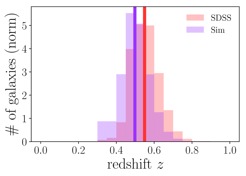
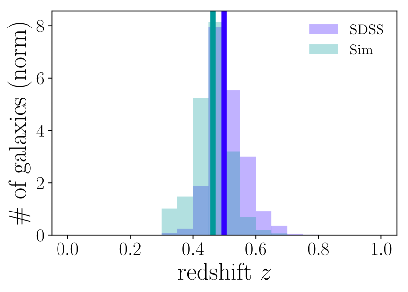
Figure 8: Spectroscopic redshift distribution (n$(z)$) for red (left panel), and blue (right panel) galaxies. Vertical lines represent the medians of their respective distribution of matching color. Red galaxies show a difference in their medians of $\Delta z_{\mathrm{red}}=0.052$, while blue galaxies have $\Delta z_{\mathrm{blue}}=0.035$.

We also measure individual galaxy properties and compare those. As a first step, we compare the redshift distributions n$(z)$ for red and blue galaxies. BOSS spectroscopic redshifts have been downloaded alongside with their spectra. Our simulated spectra come from our luminosity functions, as described in our model Section. Therefore, the two redshift definitions might show a small disagreement as they have not been measured in the same way. This must be taken into account when comparing them. Figure 8 shows the distributions for red (left hand side), and blue (right hand side), galaxies. Vertical lines of the same color of their respective distributions indicate the position of their medians. The differences in the medians result in $\Delta z_{\mathrm{red}}=0.052$ for red galaxies, and $\Delta z_{\mathrm{blue}}=0.035$ for blue galaxies. These small differences in the redshift distributions can be also used to test the performances of the model presented in [23], and can be confronted to their Figure 13.

As explained in Section 5.3.2, we also measure stellar population properties for both red and blue galaxies, on data and simulations, and we compare the property distributions. In Figure 9, we show the comparison between stellar ages, stellar metallicities, and mass-to-light ratios in the $r-$band, for our real and simulated spectra. Stellar properties appear to be very similar for red and blue galaxies. This is due to the fact that CMASS Sparse is a sub-sample of CMASS. The similarity between the two samples is also clearly visible in Figure 4.

On the left hand side of Figure 9, red galaxy stellar population properties are shown. Stellar ages appear to be centered at about 9-10 Gyrs, as expected for galaxies at these redshifts [38]. Real and simulated spectra show very good overlap. We find such high values for stellar ages also for blue galaxies not only because CMASS Sparse is a subsample of CMASS, but also because during the full spectral fitting we masked regions where emission lines coming from gas were dominant, avoiding in such way to be dominated by this effect when deriving stellar properties. The stellar ages derived here can be also compared to those derived through SED fitting in [77], with the caveats that different methodologies and choice of templates may lead to different results when deriving stellar population parameters. However, the values we report here are in the same range of those derived in that study.

An excellent agreement can be seen also for stellar metallicities, for both showing a double population peaked at values of slightly sub-solar metallicities, and very low (sub-solar) metallicities. This is in agreement with studies of CMASS galaxies, as stated for example in [77], where red galaxies never reach solar metallicity values.

A good overlap is also shown for the mass-to-light ($r-$band) ratio, with simulated galaxies showing a small shift towards lower values. The same considerations can be drawn for the blue galaxies population, with a slightly more marked disagreement for the mass-to-light ratio values.

The agreement between our real and simulated galaxies, already visible from the PCA statistical analysis, is therefore also confirmed by looking at individual stellar galaxy population properties, further strengthening our considerations about the goodness of the model presented in [23], and our technique in simulating galaxy spectra.

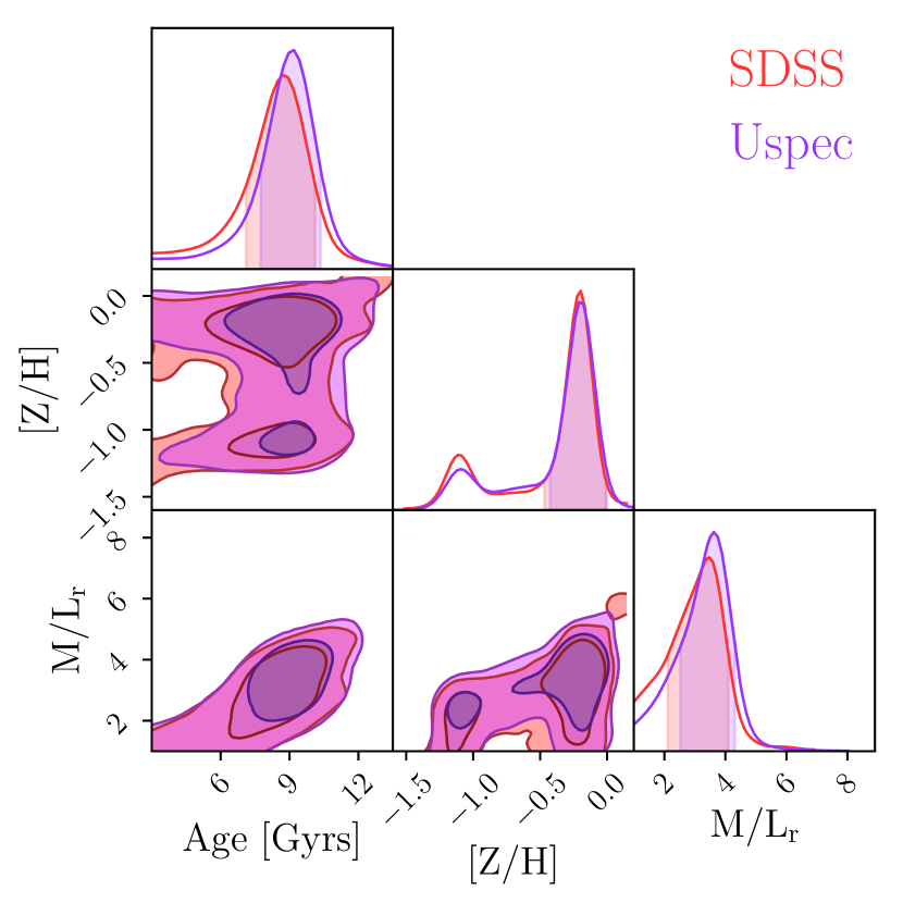
Figure 9: Stellar population properties comparison for red (left panel) and blue (right panel) between real and simulated galaxies. We show stellar ages (in Gyrs), total metallicity ([Z/H]), and Mass to Light ratios in the $r-$band (M/L_r).

7 Discussion on Forward Modeling

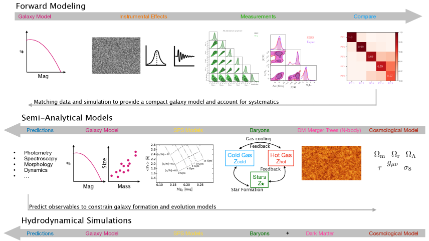
Figure 10: Synopsis of the different approaches used to model the galaxy population. Our forward modeling approach, as well as semi-analytical models and hydrodynamical simulations are shown. Forward modeling (top row) starts from a galaxy model, then includes instrumental parameters, and measurements of galaxy properties on data and simulations which are compared statistically. If the agreement between data and simulations is not sufficient, the process is repeated using modified input parameters. The process takes about a few hours on a supercomputer in our case. The second and third rows show the semi-analytical and the hydro-simulations approaches. In semi-analytical models, a cosmological model is first chosen. Then, using N-body simulations, the merger trees of dark matter halos of different masses are traced. At this point, baryons are inserted in the model together with the effects they give rise to such as hot gas cooling, cold gas conversion into stars, and feedback. This is translated into galaxy properties thorough Stellar Population Synthesis (SPS) codes. A complex, physically motivated galaxy formation and evolution model can then be developed, and different predictions about galaxy and gas properties, metallicity, temperature, initial mass function, dynamics, and morphology can be made. In hydrodynamical simulations, a cosmology is also chosen as a first step. The density fields of dark and baryonic matter are modeled. The evolution of these density fields is followed by solving numerically gravitational and hydrodynamical equations using prescriptions for baryonic physics. As well as semi-analytical models, they provide a wide-range of predictions on galaxy formation and evolution.

As the analysis presented above shows promising results, we discuss here our forward modeling technique and how it compares to other approaches.

Our analysis makes use of a simpler model for the galaxy population than the models used in semi-analytical models such as [4, 78, 79, 80, 81, 82, 83] or in hydrodynamical simulations such as [84, 85]. As illustrated in Figure 10 and described in Section 2, we indeed use a galaxy population model as an input. This includes prescriptions for the luminosity functions of red and blue galaxies, as well as a simple model for galaxy sizes and SED distribution functions, as described in [23]. In [23], it was shown that these prescriptions are successful in reproducing current observations taken from [86, 87, 88, 89, 90, 91, 45]. A question that arises is how this simple model performs for further properties which are notoriously difficult to reproduce, such as stellar ages, stellar metallicities, and mass-to-light ratios. In our approach, these properties are not inputs in the model, but they are measured after the fact in simulations and data. Therefore, we do not necessarily measure intrinsic stellar properties, but we show how our simulated sample is statistically similar to a real BOSS sample of spectra after accounting for all selection biases and systematics, for images and spectra.

Results presented in Figure 9 (see also Figure 3) show properties measured consistently on data and simulations, after careful modeling of the noise properties of images and spectra, and accounting for selection effects coming from possibly inconsistent definitions of magnitudes. These results show that our method provides a successful treatment of selection biases. Stellar population properties in particular are especially prone to biases, as results obtained with different techniques (full spectral fitting vs. Lick System, for example) can be different within the same data set [38]. Even when using the Lick System of spectral lines only, the use of different lines can lead to different results in absolute numbers, as shown in [38], however preserving consistent relative results (for example, in [38], smaller galaxies are consistently older than bigger galaxies, for stellar masses $10.5<\log\mathrm{M}_{*}/\mathrm{M}_{\odot}<11$, but the absolute ages change with different approaches, as shown in Table 3 in [38]).

Figure 10 shows a comparison between our forward modeling approach, and approaches based on semi-analytical models and hydrodynamical equations. This flowchart highlights the goals of the different methods. Forward modeling (top row) starts from a galaxy model, adding various instrumental parameters, then measures quantities on data and simulations, and then compares the two resulting measurement sets. If the level of agreement is not satisfactory, the process is repeated using a modified set of input parameters until an agreement is found using control loops. As the software tools involved are fast, this whole procedure can be executed within a few hours on a supercomputer. If the level of agreement cannot be reached by modifying both instrumental and galaxy population parameters, then the model is complexified and another set of control loops is started.

The second and third rows of Figure 10 illustrate the semi-analytical and hydrodynamic-simulation approaches. In semi-analytical models, a cosmological model is first chosen. Then, using N-body simulations, the merger trees of dark matter halos of different masses are traced. At this point, baryons are inserted in the model together with the effects they give rise to such as hot gas cooling, cold gas conversion into stars, and feedback. A complex, physically motivated galaxy formation and evolution model can then be developed, and different predictions about galaxy and gas properties, metallicity, temperature, initial mass function, dynamics, and morphology can be made. In hydrodynamical simulations, a cosmology is also chosen as a first step. The density fields of dark and baryonic matter are modeled by solving numerically gravitational and hydrodynamical equations. As well as semi-analytical models, hydrodynamic-simulations provide a wide-range of predictions on galaxy formation and evolution. These predictions go beyond the goals of our forward modeling scheme. Also, it should be taken into account that when differences arise in the comparison between the predictions of such models to real data, it is often difficult to attribute them to specific physical processes, or to noise, systematics or selection effects. Running these simulations is also a much slower process that in our forward modeling approach, especially when referring to hydrodynamical simulations.

In [92], the authors show the predictions of the GALFORM [93] semi-analytical galaxy formation model for the luminosities, morphologies, colours and scale-lengths of local galaxies. In order to compare their results to SDSS data, the authors needed to convert the standard GALFORM outputs into SDSS-like properties, like for example Petrosian magnitudes. Independently on how well one can make such a conversion, the effects of noise on data are important, especially when considering magnitudes in different bands. We showed in [22] that even when carefully modeling the noise in each band, it is difficult to obtain an agreement between real and simulated magnitudes. This is because modeling the effect of the noise in each band analytically is challenging. Such an effect can cause colours to be incorrectly estimated, and therefore galaxies associated to wrong categories in the colour-colour space. For example, our findings indicate that a large part of the differences in galaxy properties such as magnitudes and colours we saw in our previous galaxy model (see Figures 1 and 6 in [F18], but also abundance ratios in Appendix C) can be ascribed to measurements systematics and selection biases [F18]. This aspect can be explored by using, as a starting point, a simple galaxy model which can be complexified as needed, and which can be compared to other approaches. In this work, we applied the same procedure to compute real and simulated magnitudes at the image level. Therefore, with our current method we can safely assume that our residual differences between data and simulations are coming from the model rather than other effects.

Forward modeling is therefore meant to be a complementary approach to semi-analytical models and hydrodynamical simulations. The two latter approaches provide a more detailed modeling of the galaxy population, but are computationally slower than our approach which provides a detailed treatment of instrumental and selection effects. Our approach thus provides a compact, simple galaxy population model which is corrected for systematic effects and can be a useful input for comparison with the other approaches.

8 Conclusions

In this paper, we present a method to forward model a spectroscopic galaxy survey, using a target selection based on a simulated wide field imaging survey. This method can be used to simulate both red and blue galaxies.

We start from a galaxy population model which provides us with luminosity function parameters. Luminosity functions are different for red and blue galaxies. From those distributions, we draw magnitudes, redshifts and spectral coefficients, which constitute the basis for the construction of our simulated images and spectra. We then simulate a SDSS-like imaging survey with Ufig, using 157,000 images coming from the DR14 sample. We pre-process and analyse the images to derive all the parameters needed to simulate SDSS-like images. This whole analysis and simulation only take up to $\sim 4$h with 1,000 cores of a supercomputer. We simulate SDSS-like images with our fast image simulator, Ufig. We then apply selection cuts to both data and simulations. This is a particularly important step, as this allows us to avoid biases coming from different definitions of magnitudes or star-galaxy separation. We apply cuts with using our own measured magnitudes, corrected for PSF effects, and CLASS_STAR parameters coming from SExtractor.

We then retrieve SDSS/BOSS DR14 spectra. We simulate their analogs with our own built-in software devoted to that, called Uspec. We repeat the same procedure for what we call the red galaxy sample, constructed with emulating the CMASS sample cuts, and what we call the blue galaxy sample, which we obtained by following the CMASS Sparse sample cuts, a bluer subsample of the parent CMASS.

We use two main procedures to compare our populations of real and simulated galaxies. By using PCA, we compare the main statistical properties of the different samples. The first two principal components, which encode most of the information regarding the galaxy population shape of the spectrum, show very good agreement for both red and blue galaxies. The same can be said for the distribution of all the eigencoefficients, which are centered to each other and have the same width. Differences arise when looking at higher order principal components, which are more sensitive to the features of individual galaxies. These differences appear to be more pronounced for blue galaxies, as expected by the notorious difficulty to simulate their individual emission features. Also, differences in the noise properties might be relevant for higher order principal components, especially for blue galaxies, which have a lower number statistics than red galaxies.

We then compare the redshift distribution n($z$) of red and blue galaxies, finding good agreement overall but small differences in their medians. Also, we measure individual stellar population properties with pPXF, namely stellar ages, stellar metallicities and stellar masses, for both red and blue galaxies, finding very good agreement for both, and values in agreements with previous CMASS studies.

These results are a clear indication that our galaxy population model not only works for the wide-field imaging surveys it has been designed for, but also on completely independent spectroscopic data.

Our ability to reproduce realistic galaxy spectra for both red and blue galaxies offers very good prospects for future spectroscopic redshift surveys. Not only the inclusion of galaxy clustering properties can be used for cosmology applications, but the realistic stellar population properties we are able to reproduce can be used to connect clustering to studies of galaxy formation and evolution.

References

- [1] P. Collaboration, N. Aghanim, Y. Akrami, M. Ashdown, J. Aumont, C. Baccigalupi et al., Planck 2018 results. vi. cosmological parameters, 2018.
- [2] D. J. Eisenstein, I. Zehavi, D. W. Hogg, R. Scoccimarro, M. R. Blanton, R. C. Nichol et al., Detection of the Baryon Acoustic Peak in the Large-Scale Correlation Function of SDSS Luminous Red Galaxies, The Astrophysical Journal 633 (Nov., 2005) 560–574, [astro-ph/0501171].
- [3] H.-J. Seo and D. J. Eisenstein, Probing Dark Energy with Baryonic Acoustic Oscillations from Future Large Galaxy Redshift Surveys, The Astrophysical Journal 598 (Dec, 2003) 720–740, [astro-ph/0307460].
- [4] S. D. M. White and M. J. Rees, Core condensation in heavy halos: a two-stage theory for galaxy formation and clustering., Monthly Notices of the Royal Astronomical Society 183 (May, 1978) 341–358.
- [5] G. R. Blumenthal, S. M. Faber, J. R. Primack and M. J. Rees, Formation of galaxies and large-scale structure with cold dark matter., Nature 311 (Oct, 1984) 517–525.
- [6] M. Davis, G. Efstathiou, C. S. Frenk and S. D. M. White, The evolution of large-scale structure in a universe dominated by cold dark matter, The Astrophysical Journal 292 (May, 1985) 371–394.
- [7] D. J. Eisenstein, J. Annis, J. E. Gunn, A. S. Szalay, A. J. Connolly, R. C. Nichol et al., Spectroscopic Target Selection for the Sloan Digital Sky Survey: The Luminous Red Galaxy Sample, Astronomical Journal 122 (Nov., 2001) 2267–2280, [astro-ph/0108153].
- [8] B. J. Weiner, A. C. Phillips, S. M. Faber, C. N. A. Willmer, N. P. Vogt, L. Simard et al., The DEEP Groth Strip Galaxy Redshift Survey. III. Redshift Catalog and Properties of Galaxies, The Astrophysical Journal 620 (Feb., 2005) 595–617, [astro-ph/0411128].
- [9] B. Garilli, O. Le Fèvre, L. Guzzo, D. Maccagni, V. Le Brun, S. de la Torre et al., The Vimos VLT deep survey. Global properties of 20,000 galaxies in the IAB 22.5 WIDE survey, Astronomy and Astrophysics 486 (Aug., 2008) 683–695, [0804.4568].
- [10] D. Schlegel, M. White and D. Eisenstein, The Baryon Oscillation Spectroscopic Survey: Precision measurement of the absolute cosmic distance scale, in astro2010: The Astronomy and Astrophysics Decadal Survey, vol. 2010 of ArXiv Astrophysics e-prints, 2009, 0902.4680.
- [11] D. J. Eisenstein, D. H. Weinberg, E. Agol, H. Aihara, C. Allende Prieto, S. F. Anderson et al., SDSS-III: Massive Spectroscopic Surveys of the Distant Universe, the Milky Way, and Extra-Solar Planetary Systems, Astronomical Journal 142 (Sept., 2011) 72, [1101.1529].
- [12] K. S. Dawson, J.-P. Kneib, W. J. Percival, S. Alam, F. D. Albareti, S. F. Anderson et al., The SDSS-IV Extended Baryon Oscillation Spectroscopic Survey: Overview and Early Data, Astronomical Journal 151 (Feb., 2016) 44, [1508.04473].
- [13] D. J. Schlegel, R. D. Blum, F. J. Castand er, A. Dey, D. P. Finkbeiner, S. Foucaud et al., The Dark Energy Spectroscopic Instrument (DESI): The NOAO DECam Legacy Imaging Survey and DESI Target Selection, in American Astronomical Society Meeting Abstracts #225, vol. 225 of American Astronomical Society Meeting Abstracts, p. 336.07, Jan, 2015.
- [14] R. S. de Jong, O. Bellido-Tirado, C. Chiappini, É. Depagne, R. Haynes, D. Johl et al., 4MOST: 4-metre multi-object spectroscopic telescope, in Ground-based and Airborne Instrumentation for Astronomy IV, vol. 8446 of Proceedings of the SPIE, p. 84460T, Sept., 2012, 1206.6885, DOI.
- [15] H. Sugai, N. Tamura, H. Karoji, A. Shimono, N. Takato, M. Kimura et al., Prime Focus Spectrograph for the Subaru telescope: massively multiplexed optical and near-infrared fiber spectrograph, Journal of Astronomical Telescopes, Instruments, and Systems 1 (Jul, 2015) 035001, [1507.00725].
- [16] D. Masters, P. McCarthy, B. Siana, M. Malkan, B. Mobasher, H. Atek et al., Physical Properties of Emission-line Galaxies at z ~2 from Near-infrared Spectroscopy with Magellan FIRE, The Astrophysical Journal 785 (Apr, 2014) 153, [1402.0510].
- [17] G. Favole, S. A. Rodríguez-Torres, J. Comparat, F. Prada, H. Guo, A. Klypin et al., Galaxy clustering dependence on the [O II] emission line luminosity in the local Universe, Monthly Notices of the Royal Astronomical Society 472 (Nov, 2017) 550–558, [1611.05457].
- [18] A. Refregier and A. Amara, A way forward for Cosmic Shear: Monte-Carlo Control Loops, Physics of the Dark Universe 3 (Apr., 2014) 1–3, [1303.4739].
- [19] J. Herbel, T. Kacprzak, A. Amara, A. Refregier, C. Bruderer and A. Nicola, The redshift distribution of cosmological samples: a forward modeling approach, Journal of Cosmology and Astroparticle Physics 8 (Aug., 2017) 035, [1705.05386].
- [20] C. Bruderer, A. Nicola, A. Amara, A. Refregier, J. Herbel and T. Kacprzak, Cosmic shear calibration with forward modeling, ArXiv e-prints (July, 2017) , [1707.06233].
- [21] L. Tortorelli, L. Della Bruna, J. Herbel, A. Amara, A. Refregier, A. Alarcon et al., The PAU Survey: a forward modeling approach for narrow-band imaging, Journal of Cosmology and Astroparticle Physics 2018 (Nov., 2018) 035, [1805.05340].
- [22] M. Fagioli, J. Riebartsch, A. Nicola, J. Herbel, A. Amara, A. Refregier et al., Forward modeling of spectroscopic galaxy surveys: application to SDSS, Journal of Cosmology and Astroparticle Physics 11 (Nov., 2018) 015, [1803.06343].
- [23] L. Tortorelli, M. Fagioli, J. Herbel, A. Amara, T. Kacprzak and A. Refregier, Measurement of the B-band Galaxy Luminosity Function with Approximate Bayesian Computation, arXiv e-prints (Jan., 2020) arXiv:2001.07727, [2001.07727].
- [24] O. Boulade, X. Charlot, P. Abbon, S. Aune, P. Borgeaud, P.-H. Carton et al., Development of MegaCam, the next-generation wide-field imaging camera for the 3.6-m Canada-France-Hawaii Telescope, vol. 4008 of Society of Photo-Optical Instrumentation Engineers (SPIE) Conference Series, pp. 657–668. 2000. 10.1117/12.395524.
- [25] D. Burstein, S. M. Faber, C. M. Gaskell and N. Krumm, Old stellar populations. I - A spectroscopic comparison of galactic globular clusters, M31 globular clusters, and elliptical galaxies, The Astrophysical Journal 287 (Dec., 1984) 586–609.
- [26] G. Worthey, S. M. Faber, J. J. Gonzalez and D. Burstein, Old stellar populations. 5: Absorption feature indices for the complete LICK/IDS sample of stars, Astrophysical Journal, Supplement 94 (Oct., 1994) 687–722.
- [27] G. Worthey and D. L. Ottaviani, H and H Absorption Features in Stars and Stellar Populations, Astrophysical Journal, Supplement 111 (Aug, 1997) 377–386.
- [28] S. C. Trager, G. Worthey, S. M. Faber, D. Burstein and J. J. González, Old Stellar Populations. VI. Absorption-Line Spectra of Galaxy Nuclei and Globular Clusters, Astrophysical Journal, Supplement 116 (1998) 1–28, [astro-ph/9712258].
- [29] S. C. Trager, S. M. Faber, G. Worthey and J. J. González, The Stellar Population Histories of Local Early-Type Galaxies. I. Population Parameters, Astronomical Journal 119 (Apr, 2000) 1645–1676, [astro-ph/0001072].
- [30] S. C. Trager, G. Worthey, S. M. Faber and A. Dressler, Hot stars in old stellar populations: a continuing need for intermediate ages, Monthly Notices of the Royal Astronomical Society 362 (Sep, 2005) 2–8, [astro-ph/0506336].
- [31] A. J. Korn, C. Maraston and D. Thomas, The sensitivity of Lick indices to abundance variations, Astronomy and Astrophysics 438 (Aug, 2005) 685–704, [astro-ph/0504574].
- [32] B. M. Poggianti, A. Bressan and A. Franceschini, Star Formation and Selective Dust Extinction in Luminous Starburst Galaxies, The Astrophysical Journal 550 (Mar, 2001) 195–203, [astro-ph/0011160].
- [33] D. Thomas, C. Maraston and R. Bender, Stellar population models of Lick indices with variable element abundance ratios, Monthly Notices of the Royal Astronomical Society 339 (Mar, 2003) 897–911, [astro-ph/0209250].
- [34] D. Thomas and C. Maraston, The impact of alpha /Fe enhanced stellar evolutionary tracks on the ages of elliptical galaxies, Astronomy and Astrophysics 401 (Apr, 2003) 429–432, [astro-ph/0302063].
- [35] R. P. Schiavon, Population Synthesis in the Blue. IV. Accurate Model Predictions for Lick Indices and UBV Colors in Single Stellar Populations, Astrophysical Journal, Supplement 171 (Jul, 2007) 146–205, [astro-ph/0611464].
- [36] D. Thomas, C. Maraston and J. Johansson, Flux-calibrated stellar population models of Lick absorption-line indices with variable element abundance ratios, Monthly Notices of the Royal Astronomical Society 412 (Apr., 2011) 2183–2198, [1010.4569].
- [37] M. Onodera, A. Renzini, M. Carollo, M. Cappellari, C. Mancini, V. Strazzullo et al., Deep Near-infrared Spectroscopy of Passively Evolving Galaxies at z ~ 1.4, The Astrophysical Journal 755 (Aug., 2012) 26, [1206.1540].
- [38] M. Fagioli, C. M. Carollo, A. Renzini, S. J. Lilly, M. Onodera and S. Tacchella, Minor Mergers or Progenitor Bias? The Stellar Ages of Small and Large Quenched Galaxies, The Astrophysical Journal 831 (Nov., 2016) 173, [1607.03493].
- [39] P. Ocvirk, C. Pichon, A. Lançon and E. Thiébaut, STECKMAP: STEllar Content and Kinematics from high resolution galactic spectra via Maximum A Posteriori, Monthly Notices of the Royal Astronomical Society 365 (Jan, 2006) 74–84, [astro-ph/0507002].
- [40] P. Ocvirk, C. Pichon, A. Lançon and E. Thiébaut, STECMAP: STEllar Content from high-resolution galactic spectra via Maximum A Posteriori, Monthly Notices of the Royal Astronomical Society 365 (Jan, 2006) 46–73, [astro-ph/0505209].
- [41] M. Koleva, P. Prugniel, A. Bouchard and Y. Wu, ULySS: a full spectrum fitting package, Astronomy and Astrophysics 501 (Jul, 2009) 1269–1279, [0903.2979].
- [42] M. Cappellari and E. Emsellem, Parametric Recovery of Line-of-Sight Velocity Distributions from Absorption-Line Spectra of Galaxies via Penalized Likelihood, Publications of the ASP 116 (Feb., 2004) 138–147, [astro-ph/0312201].
- [43] J. Bergé, L. Gamper, A. Réfrégier and A. Amara, An Ultra Fast Image Generator (UFIG) for wide-field astronomy, Astronomy and Computing 1 (Feb., 2013) 23–32, [1209.1200].
- [44] R. Johnston, Shedding light on the galaxy luminosity function, Astronomy and Astrophysics Reviews 19 (Aug., 2011) 41, [1106.2039].
- [45] R. Beare, M. J. I. Brown, K. Pimbblet, F. Bian and Y.-T. Lin, The iz/i 1.2 Optical Luminosity Function from a Sample of 410,000 Galaxies in Bo#1255tes, The Astrophysical Journal 815 (Dec., 2015) 94, [1511.01580].
- [46] N. Balakrishnan, Handbook of the Logistic Distribution. Statistics: A Series of Textbooks and Monographs. Taylor & Francis, 2013.
- [47] M. R. Blanton, D. J. Schlegel, M. A. Strauss, J. Brinkmann, D. Finkbeiner, M. Fukugita et al., New York University Value-Added Galaxy Catalog: A Galaxy Catalog Based on New Public Surveys, Astronomical Journal 129 (June, 2005) 2562–2578, [astro-ph/0410166].
- [48] M. R. Blanton and S. Roweis, K-Corrections and Filter Transformations in the Ultraviolet, Optical, and Near-Infrared, Astronomical Journal 133 (Feb., 2007) 734–754, [astro-ph/0606170].
- [49] G. Bruzual and S. Charlot, Stellar population synthesis at the resolution of 2003, Monthly Notices of the Royal Astronomical Society 344 (Oct., 2003) 1000–1028, [astro-ph/0309134].
- [50] L. J. Kewley, M. A. Dopita, R. S. Sutherland, C. A. Heisler and J. Trevena, Theoretical Modeling of Starburst Galaxies, The Astrophysical Journal 556 (July, 2001) 121–140, [astro-ph/0106324].
- [51] J. Akeret, A. Refregier, A. Amara, S. Seehars and C. Hasner, Approximate Bayesian computation for forward modeling in cosmology, Journal of Cosmology and Astroparticle Physics 2015 (Aug, 2015) 043, [1504.07245].
- [52] P. Schechter, An analytic expression for the luminosity function for galaxies., The Astrophysical Journal 203 (Jan., 1976) 297–306.
- [53] J. E. Gunn, W. A. Siegmund, E. J. Mannery, R. E. Owen, C. L. Hull, R. F. Leger et al., The 2.5 m Telescope of the Sloan Digital Sky Survey, Astronomical Journal 131 (Apr., 2006) 2332–2359, [astro-ph/0602326].
- [54] Gaia Collaboration, VizieR Online Data Catalog: Gaia DR1 (Gaia Collaboration, 2016), VizieR Online Data Catalog (Jun, 2016) I/337.
- [55] Gaia Collaboration, VizieR Online Data Catalog: Gaia DR2 (Gaia Collaboration, 2018), VizieR Online Data Catalog (Apr, 2018) I/345.
- [56] F. Ochsenbein, P. Bauer and J. Marcout, The VizieR database of astronomical catalogues, Astronomy and Astrophysics, Supplement 143 (Apr, 2000) 23–32, [astro-ph/0002122].
- [57] E. Bertin, Y. Mellier, M. Radovich, G. Missonnier, P. Didelon and B. Morin, The TERAPIX Pipeline, vol. 281 of Astronomical Society of the Pacific Conference Series, p. 228. 2002.
- [58] E. Bertin, Automatic Astrometric and Photometric Calibration with SCAMP, vol. 351 of Astronomical Society of the Pacific Conference Series, p. 112. 2006.
- [59] E. Bertin and S. Arnouts, SExtractor: Software for source extraction., Astronomy and Astrophysics, Supplement 117 (June, 1996) 393–404.
- [60] B. Xin, Ž. Ivezić, R. H. Lupton, J. R. Peterson, P. Yoachim, R. L. Jones et al., A Study of the Point-spread Function in SDSS Images, Astronomical Journal 156 (Nov, 2018) 222, [1805.02845].
- [61] J. H. Knapen, S. Erroz-Ferrer, J. Roa, J. Bakos, M. Cisternas, R. Leaman et al., Optical imaging for the Spitzer Survey of Stellar Structure in Galaxies. Data release and notes on interacting galaxies, Astronomy and Astrophysics 569 (Sep, 2014) A91, [1406.4107].
- [62] A. Ginsburg, B. M. Sipőcz, C. E. Brasseur, P. S. Cowperthwaite, M. W. Craig, C. Deil et al., astroquery: An Astronomical Web-querying Package in Python, Astronomical Journal 157 (Mar, 2019) 98, [1901.04520].
- [63] C. Bruderer, C. Chang, A. Refregier, A. Amara, J. Bergé and L. Gamper, Calibrated Ultra Fast Image Simulations for the Dark Energy Survey, The Astrophysical Journal 817 (Jan., 2016) 25, [1504.02778].
- [64] C. Bonnett, M. A. Troxel, W. Hartley, A. Amara, B. Leistedt, M. R. Becker et al., Redshift distributions of galaxies in the Dark Energy Survey Science Verification shear catalogue and implications for weak lensing, Physical Review D 94 (Aug., 2016) 042005, [1507.05909].
- [65] B. Leistedt, H. V. Peiris, F. Elsner, A. Benoit-Lévy, A. Amara, A. H. Bauer et al., Mapping and Simulating Systematics due to Spatially Varying Observing Conditions in DES Science Verification Data, Astrophysical Journal, Supplement 226 (Oct., 2016) 24, [1507.05647].
- [66] T. Kacprzak, J. Herbel, A. Nicola, R. Sgier, F. Tarsitano, C. Bruderer et al., Monte Carlo Control Loops for cosmic shear cosmology with DES Year 1, arXiv e-prints (Jun, 2019) arXiv:1906.01018, [1906.01018].
- [67] J. E. O’Donnell, Rnu-dependent optical and near-ultraviolet extinction, The Astrophysical Journal 422 (Feb., 1994) 158–163.
- [68] D. J. Schlegel, D. P. Finkbeiner and M. Davis, Maps of Dust Infrared Emission for Use in Estimation of Reddening and Cosmic Microwave Background Radiation Foregrounds, The Astrophysical Journal 500 (June, 1998) 525–553, [astro-ph/9710327].
- [69] D. Coe, N. Benítez, S. F. Sánchez, M. Jee, R. Bouwens and H. Ford, Galaxies in the Hubble Ultra Deep Field. I. Detection, Multiband Photometry, Photometric Redshifts, and Morphology, Astronomical Journal 132 (Aug, 2006) 926–959, [astro-ph/0605262].
- [70] K. S. Dawson, D. J. Schlegel, C. P. Ahn, S. F. Anderson, É. Aubourg, S. Bailey et al., The Baryon Oscillation Spectroscopic Survey of SDSS-III, Astronomical Journal 145 (Jan., 2013) 10, [1208.0022].
- [71] A. J. Connolly, A. S. Szalay, M. A. Bershady, A. L. Kinney and D. Calzetti, Spectral Classification of Galaxies: an Orthogonal Approach, Astronomical Journal 110 (Sept., 1995) 1071, [astro-ph/9411044].
- [72] M. Cappellari, Improving the full spectrum fitting method: accurate convolution with Gauss-Hermite functions, Monthly Notices of the Royal Astronomical Society 466 (Apr., 2017) 798–811, [1607.08538].
- [73] A. Vazdekis, M. Koleva, E. Ricciardelli, B. Röck and J. Falcón-Barroso, UV-extended E-MILES stellar population models: young components in massive early-type galaxies, Monthly Notices of the Royal Astronomical Society 463 (Dec, 2016) 3409–3436, [1612.01187].
- [74] A. D. Bolatto, J. M. Jackson and J. G. Ingalls, A Semianalytical Model for the Observational Properties of the Dominant Carbon Species at Different Metallicities, The Astrophysical Journal 513 (Mar, 1999) 275–286, [astro-ph/9812181].
- [75] M. Röllig, V. Ossenkopf, S. Jeyakumar, J. Stutzki and A. Sternberg, [CII] 158 m emission and metallicity in photon dominated regions, Astronomy and Astrophysics 451 (Jun, 2006) 917–924, [astro-ph/0601682].
- [76] K. Olsen, A. Pallottini, A. Wofford, M. Chatzikos, M. Revalski, F. Guzmán et al., Challenges and Techniques for Simulating Line Emission, Galaxies 6 (Sep, 2018) 100, [1808.08251].
- [77] C. Maraston, J. Pforr, B. M. Henriques, D. Thomas, D. Wake, J. R. Brownstein et al., Stellar masses of SDSS-III/BOSS galaxies at z 0.5 and constraints to galaxy formation models, Monthly Notices of the Royal Astronomical Society 435 (Nov., 2013) 2764–2792, [1207.6114].
- [78] S. D. M. White and C. S. Frenk, Galaxy Formation through Hierarchical Clustering, The Astrophysical Journal 379 (Sept., 1991) 52.
- [79] C. M. Baugh, A primer on hierarchical galaxy formation: the semi-analytical approach, Reports on Progress in Physics 69 (Dec., 2006) 3101–3156, [astro-ph/0610031].
- [80] A. J. Benson and R. Bower, Galaxy formation spanning cosmic history, Monthly Notices of the Royal Astronomical Society 405 (July, 2010) 1573–1623, [1003.0011].
- [81] A. J. Benson, Galaxy formation theory, Reports on Progress in Physics 495 (Oct., 2010) 33–86, [1006.5394].
- [82] P. Monaco, A. J. Benson, G. De Lucia, F. Fontanot, S. Borgani and M. Boylan-Kolchin, A semi-analytic model comparison: testing cooling models against hydrodynamical simulations, Monthly Notices of the Royal Astronomical Society 441 (July, 2014) 2058–2077, [1404.0811].
- [83] J. Hou, C. G. Lacey and C. S. Frenk, A comparison between semi-analytical gas cooling models and cosmological hydrodynamical simulations, Monthly Notices of the Royal Astronomical Society 486 (June, 2019) 1691–1717, [1803.01923].
- [84] M. Vogelsberger, S. Genel, V. Springel, P. Torrey, D. Sijacki, D. Xu et al., Properties of galaxies reproduced by a hydrodynamic simulation, Nature 509 (May, 2014) 177–182, [1405.1418].
- [85] J. Schaye, R. A. Crain, R. G. Bower, M. Furlong, M. Schaller, T. Theuns et al., The EAGLE project: simulating the evolution and assembly of galaxies and their environments, Monthly Notices of the Royal Astronomical Society 446 (Jan., 2015) 521–554, [1407.7040].
- [86] E. Giallongo, S. Salimbeni, N. Menci, G. Zamorani, A. Fontana, M. Dickinson et al., The B-Band Luminosity Function of Red and Blue Galaxies up to z = 3.5, The Astrophysical Journal 622 (Mar, 2005) 116–128, [astro-ph/0412044].
- [87] O. Ilbert, S. Lauger, L. Tresse, V. Buat, S. Arnouts, O. Le Fèvre et al., The VIMOS-VLT Deep Survey. Galaxy luminosity function per morphological type up to z = 1.2, Astronomy and Astrophysics 453 (Jul, 2006) 809–815, [astro-ph/0604010].
- [88] E. Zucca, S. Bardelli, M. Bolzonella, G. Zamorani, O. Ilbert, L. Pozzetti et al., The zCOSMOS survey: the role of the environment in the evolution of the luminosity function of different galaxy types, Astronomy and Astrophysics 508 (Dec, 2009) 1217–1234, [0909.4674].
- [89] J. Loveday, P. Norberg, I. K. Baldry, S. P. Driver, A. M. Hopkins, J. A. Peacock et al., Galaxy and Mass Assembly (GAMA): ugriz galaxy luminosity functions, Monthly Notices of the Royal Astronomical Society 420 (Feb, 2012) 1239–1262, [1111.0166].
- [90] R. J. Cool, D. J. Eisenstein, C. S. Kochanek, M. J. I. Brown, N. Caldwell, A. Dey et al., The Galaxy Optical Luminosity Function from the AGN and Galaxy Evolution Survey, The Astrophysical Journal 748 (Mar, 2012) 10, [1201.2954].
- [91] A. Fritz, M. Scodeggio, O. Ilbert, M. Bolzonella, I. Davidzon, J. Coupon et al., The VIMOS Public Extragalactic Redshift Survey (VIPERS):. A quiescent formation of massive red-sequence galaxies over the past 9 Gyr, Astronomy and Astrophysics 563 (Mar, 2014) A92, [1401.6137].
- [92] J. E. González, C. G. Lacey, C. M. Baugh, C. S. Frenk and A. J. Benson, Testing model predictions of the cold dark matter cosmology for the sizes, colours, morphologies and luminosities of galaxies with the SDSS, Monthly Notices of the Royal Astronomical Society 397 (Aug., 2009) 1254–1274, [0812.4399].
- [93] S. Cole, A. Benson, C. Baugh, C. Lacey and C. Frenk, The Evolution of Galaxy Clustering in Hierachical Models, vol. 200 of Astronomical Society of the Pacific Conference Series, p. 109. 2000.