Irvsp: to obtain irreducible representations of electronic states in the VASP

Abstract

We present an open-source program irvsp, to compute irreducible representations of electronic states for all 230 space groups with an interface to the Vienna ab-initio Simulation Package. This code is fed with plane-wave-based wavefunctions (e.g. WAVECAR) and space group operators (listed in OUTCAR), which are generated by the VASP package. This program computes the traces of matrix presentations and determines the corresponding irreducible representations for all energy bands and all the $k$-points in the three-dimensional Brillouin zone. It also works with spin-orbit coupling (SOC), i.e., for double groups. It is in particular useful to analyze energy bands, their connectivities, and band topology, after the establishment of the theory of topological quantum chemistry. Accordingly, the associated library -- irrep_bcs.a -- is developed, which can be easily linked to by other ab-initio packages. In addition, the program has been extended to orthogonal tight-binding (TB) Hamiltonians, e.g. electronic or phononic TB Hamiltonians. A sister program ir2tb is presented as well.
Program summary
Program title: irvsp
Program Files doi: https://doi.org/10.17632/y9ds5nnm2f.1
Licensing provisions: GNU Lesser General Public License, https://www.gnu.org/licenses/lgpl-3.0.html
Distribution format: tar.gz
Programming language: Fortran 90/77
Computer: Any architecture with a Fortran 90 complier
RAM: 20 MB
Nature of problem: Determining irreducible representations for all energy bands and all the $k$-points in 230 space groups. It is in particular useful to analyze energy bands, their connectivities, and band topology.
Solution method: By computing the traces of matrix presentations of space group operators for the eigen-wavefunctions at a certain $k$-point in a given space group, one can determine irreducible representations for them.
Running time: It takes less than 1 minute for the calculation of Bismuth.
Keywords
Irreducible representations; First-principles calculations; Nonsymmorphic space groups; Plane-wave basis; Tight-binding Hamiltonian; Topological materials

I Introduction

Topological states have been intensively studied in the past decades Bernevig et al. (2006); König et al. (2007); Kane and Mele (2005); Bernevig and Zhang (2006); Kane and Hasan (2010); Qi and Zhang (2011); Schindler et al. (2018); Wan et al. (2011); Wieder et al. (2018). During the period, lots of materials have theoretically been proposed to be topological insulators and topological semimetals, based on calculations within the density-functional theory (DFT) Tang et al. (2019); Zhang et al. (2019); Vergniory et al. (2019); Xu et al. (2019); Li et al. (2017); Nie et al. (2018); Qian et al. (2019). Many of them are verified in experiments, and substantially intrigue much interest in theories and experiments, such as three-dimensional (3D) topological insulator Bi₂Se₃ Zhang et al. (2009); Xia et al. (2009); Chen et al. (2009), Dirac semimetals Na₃Bi Wang et al. (2012); Liu et al. (2014a) and Cd₃As₂ Wang et al. (2013); Liu et al. (2014b), Weyl semimetal TaAs Weng et al. (2015); Huang et al. (2015); Lv et al. (2015); Xu et al. (2015), topological crystalline insulator SnTe Hsieh et al. (2012); Tanaka et al. (2012) and hourglass material KHgSb Wang et al. (2016); Ma et al. (2017) et al. To some extent, these topological electron bands are related to a band-inversion feature. Explicitly, there can be a band inversion between different irreducible representations (IRs) of the little groups at $k$-points in the 3D Brillouin zone (BZ) Zhu et al. (2012). In the situation of Dirac semimetals or nodal-line semimetals, the band inversion may happen on a high-symmetry line or in a high-symmetry plane.

Very recently, new insights about band theory have been used to classify all the nontrivial electron band topologies compatible with a given crystal structure Po et al. (2017); Song et al. (2018); Kruthoff et al. (2017); Bradlyn et al. (2017). In particular, based on the theory of topological quantum chemistry (TQC) Bradlyn et al. (2017); Cano et al. (2018a); Vergniory et al. (2017); Cano et al. (2018b), the topology of a set of isolated electron bands is relied on IRs at the maximal high-symmetry $k$-points (HSK), as the compatibility relations are obtained in Ref. Elcoro et al. (2017), and open accessible on the Bilbao Crystallographic Server (BCS) Aroyo et al. (2011); Stokes et al. (2013). The set of maximal HSK points can be found by using the BCS. The determination of the IRs of electron bands at maximal HSK points is of great interest, for which the program – vasp2trace – was developed Vergniory et al. (2019). However, it is not suitable for any non-maximal HSK points.

Generally speaking, in order to obtain the IRs for electron energy bands in crystals, two ingredients are necessary: a) wave-functions (WFs) at $k$-points and b) character tables (CRTs) for $k$-little groups. Different versions of the codes can be developed based on the different types of the WFs and conventions of the CRTs. The program irrep in the WIEN2k package Blaha et al. (2001); Persson (1999) is a precursor in determining the IRs, which is based on the plane-wave (PW) basis (the part of the WFs outside muffin-tin spheres) and the CRTs of 32 point groups (PNGs). There is an advantage of describing the IRs in terms of the more well-known PNG symmetries; however, the disadvantage is that in many cases $k$-points on the BZ surface cannot be classified with PNGs for nonsymmorphic crystals. In this paper, the program – irvsp – is developed based on the CRTs on the BCS. It originates from the WIEN2k irrep code Blaha et al. (2001); Persson (1999) that considers both single and double groups, analyses of time-reversal symmetry, and handles accidental degeneracies. The present code inherits those features but it has been extended to also be able to determine IRs of those special $k$-points for nonsymmorphic crystals. Hence, the code labels the IRs according to the convention of the BCS notation Stokes et al. (2013) for 230 space groups (SGs). In fact, it works for 1651 magnetic space groups (MSGs), once the space group number of the unitary part of MSGs is correctly given. In addition, Wannier-based tight-binding (TB) models are widely used to study the topological properties of real materials, including topological surface states and symmetry indicators. To get the band representations and check the topology of these models, a sister program – ir2tb – is developed to interface with orthogonal TB Hamiltonians, e.g. electronic or phononic TB Hamiltonians.

This paper is organized as follows. In Section II, we present some basic derivations to compute the traces of matrix presentations (MPs) in different bases. In Section III, we introduce the general process of the code. In Section IV, we introduce the capabilities of this package. In Section V, we introduce the installation and basic usages. In Section VI, we introduce some examples in order to show how to use irvsp to determine the IRs and further explore the topology.

II Methods

Space-group operations (SGOs), ${\cal O}_{s}=\{R_{s}|{\bf v}_{s}\}$, are consist of two parts: a rotation part $R_{s}$ and a translation part ${\bf v}_{s}$. The product of two operations is defined as $\{R_{s}|{\bf v}_{s}\}\{R_{t}|{\bf v}_{t}\}=\{R_{s}R_{t}|R_{s}{\bf v}_{t}+{\bf v}_{s}\}$. An operator acting on a scalar function in real space is expressed by ${\cal O}_{s}f({\bf r})=f({\cal O}_{s}^{-1}{\bf r})=f(R_{s}^{-1}{\bf r}-R_{s}^{-1}{\bf v}_{s})$ (There is a typo in Section A of the supplementary information of Ref. Vergniory et al. (2019)). The MPs, $O_{s}^{mn}$, can be computed in the basis of the Bloch wavefunctions $\left|\psi_{n\bf k}\right\rangle$: $O_{s}^{mn}=\left\langle\psi_{m\bf k}|{\cal O}_{s}|\psi_{n\bf k}\right\rangle$. The traces of the obtained MPs are the characters, and they are essential to determine the corresponding IRs of the little group (LG) of ${\bf k}$. The LG of ${\bf k}$ [$LG(k)$] is defined as a set of SGOs:

$$LG(k):~{}\{{\cal O}_{s}|R_{s}{\bf k}={\bf k}+{\bf G}\},\text{ with }{\bf G}=l{\bf g}_{1}+m{\bf g}_{2}+n{\bf g}_{3},~{}l,m,n\in\mathbb{N}$$ (1)

Here, ${\bf G}$ could be any integer reciprocal lattice translation (${\bf g}_{1},{\bf g}_{2},{\bf g}_{3}$ are primitive reciprocal lattice vectors). The traces of MPs of SGOs are defined as:

$$\text{Tr}[{\cal O}_{s}]=\sum_{n}O_{s}^{nn}\text{ with }O_{s}^{nn}=\left\langle\psi_{n\bf k}|{\cal O}_{s}|\psi_{n\bf k}\right\rangle,~{}{\cal O}_{s}\in LG(k).$$ (2)

Here, the WFs have to be normalized (i.e., $\left\langle\psi_{n\bf k}|\psi_{n\bf k}\right\rangle=1$).

Under different bases, the WFs can be expressed in different ways, and the derivations of Eq. (2) are different. Here, we have derived the expressions in two bases: i) PW basis and ii) TB basis. In what follows, symbols in the bold text are vectors, and common braket notations are employed:

$$\left\langle{\bf r}|A\right\rangle \equiv A({\bf r})$$

$$\left\langle A|B\right\rangle \equiv \int d{\bf r}A^{*}({\bf r})B({\bf r})$$

$$\left\langle{\bf r}|{\bf k}\right\rangle \equiv e^{i{\bf k}\cdot{\bf r}}$$

To be convenient, we present the derivations in the cases without the spin degree of freedom. However, the derivations can be easily extended to the cases including SOC, by substituting $R_{s}\otimes SU_{s}(2)$ for $R_{s}$, where the bases are doubled by the direct product: $\{{\rm PW/TB}~{}basis\}\otimes\{\left|\uparrow\right\rangle,\left|\downarrow\right\rangle\}$. In fact, the code works for both single and double groups.

II.1 Plane-wave basis

In the PW basis, wavefunctions/eigenstates are expressed in the basis of plane waves:

$$\psi_{n\bf k}({\bf r})=\sum_{j}C_{{\bf k},j}e^{i({\bf k}+{\bf G}_{j})\cdot{\bf r}}\text{ with }\left\langle{\bf k}+{\bf G}_{i}|{\bf k}+{\bf G}_{j}\right\rangle=\delta_{ij}$$ (3)

The coefficients ($C_{{\bf k},j}$) are usually computed in the ab-initio calculations and output by the DFT package (e.g. VASP, PWscf, etc.). The SGOs acting on WFs are derived as:

$${\cal O}_{s}\psi_{n\bf k}({\bf r}) = \sum_{j}C_{{\bf k},j}e^{i({\bf k}+{\bf G}_{j})\cdot(R^{-1}_{s}{\bf r}-R^{-1}_{s}{\bf v}_{s})}$$

$$= \sum_{j}C_{{\bf k},j}e^{iR_{s}({\bf k}+{\bf G}_{j})\cdot({\bf r}-{\bf v}_{s})}$$

$$= \sum_{j}C_{{\bf k},j}e^{i({\bf k}+{\bf G}_{j^{\prime}})\cdot({\bf r}-{\bf v}_{s})}\text{ with }{\bf k}+{\bf G}_{j^{\prime}}\equiv R_{s}({\bf k}+{\bf G}_{j})$$

$$= e^{-i{\bf k}\cdot{\bf v}_{s}}\sum_{j}C_{{\bf k},j}e^{-i{\bf G}_{j^{\prime}}\cdot{\bf v}_{s}}e^{i({\bf k}+{\bf G}_{j^{\prime}})\cdot{\bf r}}\text{ with }{\bf G}_{j^{\prime}}\equiv R_{s}({\bf k}+{\bf G}_{j})-{\bf k}$$

Then, Eq. (2) can be written as:

$$\left\langle\psi_{n\bf k}|{\cal O}_{s}|\psi_{n\bf k}\right\rangle = e^{-i{\bf k}\cdot{\bf v}_{s}}\sum_{j}C^{*}_{{\bf k},j^{\prime}}C_{{\bf k},j}e^{-i{\bf G}_{j^{\prime}}\cdot{\bf v}_{s}}\text{ with }{\bf G}_{j^{\prime}}\equiv R_{s}({\bf k}+{\bf G}_{j})-{\bf k}$$ (4)

The program irvsp is developed based on the above derivations with the interface to VASP Kresse and Furthmüller (1996). In addition, the library of the code is developed (see details in Appendix 6), which can be downloaded from the public code archive: https://github.com/zjwang11/irvsp/blob/master/lib_irrep_bcs.tar.gz. The library – irrep_bcs.a – can be easily linked to by other ab-initio packages, once a proper interface is made.

II.2 Orthogonal tight-binding basis

In a TB Hamiltonian, WFs are expressed in the basis of exponentially localized orthogonal orbitals: $\left|\bf{0},\mu\alpha\right\rangle\equiv\phi_{\alpha}^{\mu}({\bf r})\equiv\phi_{\alpha}({\bf r}-\tau_{\mu})$ and $\left|{\bf L}_{j},\mu\alpha\right\rangle\equiv\phi_{\alpha}({\bf r}-{\bf L}_{j}-\tau_{\mu})$, where $\mu$ label the atoms, $\alpha$ label the orbitals, ${\bf L}_{j}$ label the lattice vectors in 3D crystals, and $\tau_{\mu}$ label the positions of atoms in the home unit cell. At a given $k$-point, WFs are given as:

$$\psi_{n\bf k}({\bf r})=\sum_{\mu\alpha}C^{n}_{\mu\alpha,{\bf k}}\phi_{\alpha{\bf k}}^{\mu}({\bf r})\text{ where~{}$n$~{}is a band index},$$ (5)

$$\phi_{\alpha{\bf k}}^{\mu}({\bf r})=\sum_{j}\phi_{\alpha}({\bf r}-\tau_{\mu}-{\bf L}_{j})e^{i\mathbf{k}\cdot({\bf L}_{j}+\tau_{\mu})},\left\langle\phi_{\beta{\bf k}}^{\mu^{\prime}}|\phi_{\alpha{\bf k}}^{\mu}\right\rangle=\delta_{\mu\mu^{\prime}}\delta_{\alpha\beta}$$ (6)

The states $\phi_{\alpha{\bf k}}^{\mu}({\bf r})$ are the Fourier transformations of the local orbitals $\phi_{\alpha}^{\mu}({\bf r})$, as shown in Eq. (6). The coefficients are obtained as the eigenvectors of the TB Hamiltonian: $H_{\mu^{\prime}\beta,\mu\alpha}({\bf k})=\sum_{j}e^{i{\bf k}\cdot({\bf L}_{j}+\tau_{\mu}-\tau_{\mu^{\prime}})}\left\langle{\bf{0}},\mu^{\prime}\beta|\hat{H}|{\bf L}_{j},\mu\alpha\right\rangle$. The rotational symmetries $R_{s}$ acting on the local orbitals [$\phi_{\alpha}({\bf r})$] at the $\mu$ site are given as:

$$\widehat{R_{s}\phi}_{\alpha}({\bf r})\equiv R_{s}\phi_{\alpha}({\bf r})=\sum_{\beta}\phi_{\beta}({\bf r})D^{s,\mu}_{\beta\alpha}$$ (7)

These $D$-matrices are explicitly given in Table S3 in Appendix 2. Under the basis of real spherical harmonic functions with different total angular momenta (integer $l$), these $D$-matrices are real.

The SGOs acting on the states $\phi_{\alpha\mathbf{k}}^{\mu}({\bf r})$ are given below:

$${\cal O}_{s}\phi_{\alpha\mathbf{k}}^{\mu}({\bf r}) = \phi_{\alpha\mathbf{k}}^{\mu}(R_{s}^{-1}{\bf r}-R_{s}^{-1}{\bf v}_{s})$$

$$= \sum_{j}\phi_{\alpha}(R_{s}^{-1}{\bf r}-R_{s}^{-1}{\bf v}_{s}-\tau_{\mu}-{\bf L}_{j})e^{i\mathbf{k}\cdot({\bf L}_{j}+\tau_{\mu})}$$

$$= \sum_{j}\phi_{\alpha}(R_{s}^{-1}[{\bf r}-{\bf v}_{s}-R_{s}\tau_{\mu}-R_{s}{\bf L}_{j}])e^{i\mathbf{k}\cdot({\bf L}_{j}+\tau_{\mu})}$$

$$= \sum_{j}\widehat{R_{s}\phi}_{\alpha}[{\bf r}-{\bf v}_{s}-R_{s}\tau_{\mu}-R_{s}{\bf L}_{j}]e^{i(R_{s}\mathbf{k})\cdot R_{s}({\bf L}_{j}+\tau_{\mu})}\text{ with }\widehat{R_{s}\phi}_{\alpha}({\bf r})\equiv\sum_{\beta}\phi_{\beta}({\bf r})D^{s,\mu}_{\beta\alpha}$$

$$= e^{-i(R_{s}{\bf k}\cdot{\bf v}_{s})}\sum_{j}\widehat{R_{s}\phi}_{\alpha}[{\bf r}-({\bf v}_{s}+R_{s}\tau_{\mu})-R_{s}{\bf L}_{j}]e^{i(R_{s}\mathbf{k})\cdot[R_{s}{\bf L}_{j}+(R_{s}\tau_{\mu}+{\bf v}_{s})]}$$

$$= e^{-i(R_{s}{\bf k}\cdot{\bf v}_{s})}\sum_{j}\widehat{R_{s}\phi}_{\alpha}[{\bf r}-(\tau_{\mu^{\prime}}+{\bf L}^{i}_{0})-R_{s}{\bf L}_{j}]e^{i(R_{s}\mathbf{k})\cdot[R_{s}{\bf L}_{j}+(\tau_{\mu^{\prime}}+{\bf L}^{i}_{0})]}\text{ using }{\bf v}_{s}+R_{s}\tau_{\mu}={\bf L}^{i}_{0}+\tau_{\mu^{\prime}}$$

$$= e^{-i(R_{s}{\bf k}\cdot{\bf v}_{s})}\sum_{j^{\prime}}\widehat{R_{s}\phi}_{\alpha}[{\bf r}-\tau_{\mu^{\prime}}-{\bf L}_{j^{\prime}}]e^{i(R_{s}\mathbf{k})\cdot[{\bf L}_{j^{\prime}}+\tau_{\mu^{\prime}}]}\text{ with }{\bf L}_{j^{\prime}}={\bf L}^{i}_{0}+R_{s}{\bf L}_{j}$$

$$= e^{-i(R_{s}{\bf k}\cdot{\bf v}_{s})}\sum_{\beta}\phi_{\beta,R_{s}\mathbf{k}}^{\mu^{\prime}}(r)D^{s,\mu}_{\beta\alpha}$$

Thus, Eq. (2) is written as:

$$\left\langle\psi_{n\bf k}|{\cal O}_{s}|\psi_{n\bf k}\right\rangle = e^{-i(R_{s}{\bf k}\cdot{\bf v}_{s})}\sum_{\alpha\mu,\beta}(C^{n}_{\mu^{\prime}\beta})^{*}e^{i(R_{s}{\bf k}-{\bf k})\cdot\tau_{\mu^{\prime}}}D^{s,\mu}_{\beta\alpha}C^{n}_{\mu\alpha}\text{ with }{\bf v}_{s}+R_{s}\tau_{\mu}={\bf L}^{i}_{0}+\tau_{\mu^{\prime}}$$ (8)

In a matrix format,

$$\left\langle\psi_{n\bf k}|{\cal O}_{s}|\psi_{n\bf k}\right\rangle=e^{-i(R_{s}{\bf k}\cdot{\bf v}_{s})}\left[\overline{C^{\dagger}V(R_{s}{\bf k}-{\bf k})DC}\right]_{nn}$$ (9)

$$\text{ with }\overline{V}({\bf k})_{\mu^{\prime}\beta,\mu\alpha}=e^{i{\bf k}\cdot{\tau_{\mu}}}\delta_{\mu\mu^{\prime}}\delta_{\alpha\beta},~{}\overline{C}_{\mu\alpha,n}=C^{n}_{\mu\alpha},\overline{D}_{\mu^{\prime}\beta,\mu\alpha}=\begin{cases}\begin{array}[]{cc}D^{s,\mu}_{\beta\alpha}&\text{when }{\bf v}_{s}+R_{s}\tau_{\mu}={\bf L}^{i}_{0}+\tau_{\mu^{\prime}};\\ 0&\text{otherwise}.\end{array}\end{cases}$$ (10)

Based on the above derivations, the code has been extended to the TB basis. The sister program is called ir2tb. To run ir2tb, users must provide two files: case_hr.dat and tbbox.in. The file called case_hr.dat, containing the TB parameters, may be generated by the software Wannier90 Marzari et al. (2012); Mostofi et al. (2014) with symmetrization Wu et al. (2018); Yue ; Gresch et al. (2018), or generated by users with a toy TB model, or generated from Slater-Koster method Slater and Koster (1954) or discretization of $k\cdot p$ model onto a lattice Willatzen and Voon (2009). The other file tbbox.in is the master input file for ir2tb. It should be given consistently with the TB parameters in case_hr.dat. The tbbox.in for Bi₂Se₃ is given in Appendix 1. In addition, the example of electronic TB Hamiltonian for Bi₂Se₃ and the example of phononic TB Hamiltonian for CoSi are included in the archive src_ir2tb_v2.tar.gz.

centerlast File Description Input wave_data.f90 reading the coefficients $C_{{\bf k},j}$. WAVECAR init.f90 reading lattice vectors and space group operators, and setting up the $Z$ and $Z^{-1}$ matrices. OUTCAR kgroup.f90 determining the ${\bf k}$-little groups. nonsymm.f90 retrieving the character tables from the BCS chrct.f90 computing the traces through Eq. (4), and determining the IRs

Table 1: A brief summary of key subroutines

III General process of the code

In the main text, we are mainly focused on irvsp, which is based on the PW basis with an interface to the VASP package Kresse and Furthmüller (1996). The key subroutines are summarized in Table 1. One can check more details for ir2tb and irrep_bcs.a in the Appendix. The program ir2tb works for orthogonal TB Hamiltonians, e.g. the electronic or phononic TB Hamiltonians. The library irrep_bcs.a can be linked to by other DFT packages.

III.1 Wavefunctions at $k$-points

In the VASP package, the all-electron wave-function is obtained by acting a linear operator $\cal T$ on the pseudo-wavefunction: $\left|\psi_{n\bf k}\right\rangle={\cal T}\left|\tilde{\psi}_{n\bf k}\right\rangle$. The linear operator can be written explicitly as: ${\cal T}={\bf 1}+\sum_{i}\left(\left|\phi_{i}\right\rangle-\left|\tilde{\phi}_{i}\right\rangle\right)\left\langle p_{i}\right|$, where $\left|\phi_{i}\right\rangle$ ($\left|\tilde{\phi}_{i}\right\rangle$) is a set of all-electron (pseudo) partial waves around each atom and $\left|p_{i}\right\rangle$ is a set of corresponding projector functions on each atom within an augmentation region ($r<R_{0}$), where $R_{0}$ is the core part for each atom. The pseudo-wavefunction is expanded in the plane waves:

$$\tilde{\psi}_{n\bf k}(\vec{r})\equiv\left\langle\vec{r}|\tilde{\psi}_{n\bf k}\right\rangle=\sum_{{\bf G}_{j}}C_{n,{\bf k}+{\bf G}_{j}}e^{i({\bf k}+{\bf G}_{j})\cdot\vec{r}}$$ (11)

where ${\bf G}_{j}$ vectors are determined by the condition $\frac{\hbar^{2}}{2m_{e}}({\bf k}+{\bf G}_{j})^{2}<E_{cutoff}$ with a cutoff $E_{cutoff}$. It is worthy noting that $\left|\tilde{\psi}_{n{\bf k}}\right\rangle$ are sufficient for the calculations of the traces of MPs of SGOs.

Since the pseudo-wavefunctions $\left|\tilde{\psi}_{n{\bf k}}\right\rangle$ are usually not normalized, they have to be renormalized before their traces can be computed via Eq. (2). The coefficients ($C_{{\bf k}+{\bf G}_{j}}$) are output in WAVECAR by VASP. In the program, they are read by the subroutine: wave_data.f90. In the SOC case, the $C_{{\bf k}+{\bf G}_{j},\uparrow}$ and $C_{{\bf k}+{\bf G}_{j},\downarrow}$ are stored in the complex variables coeffa(:) and coeffb(:). In the case without SOC, the $C_{{\bf k}+{\bf G}_{j}}$ are stored in coeffa(:), while coeffb(:) are invalid (set to be zero).

III.2 Space group operators of a 3D crystal

Instead of generating space group operators from a 3D crystal structure (i.e., POSCAR), the program reads the SGOs directly from the standard output of VASP (i.e., OUTCAR), which is done by the subroutine: init.f90. In other words, the SGOs are generated by the VASP package (e.g. with ISYM = 1 or 2 in INCAR for vasp.5.3.3), which are listed below the line of ‘Space group operators:’ in OUTCAR. Fig. 1 shows an example of Bi₂Se₃ for the SGOs of space group (SG) 166. They are given by $Det~{}(\pm 1)$, $\omega$, and $\vec{n}~{}(n_{x},n_{y},n_{z})$ and ${\bf v}$ (v${}_{1}{\bf t}_{1}$,v${}_{2}{\bf t}_{2}$,v${}_{3}{\bf t}_{3}$) with ${\bf t}_{1},{\bf t}_{2},{\bf t}_{3}$ primitive lattice vectors. The $-1$ value of $Det$ indicates that the operator is a roto-inversion. Actually, the listed SGOs depend on the lattice vectors. Primitive lattice vectors (${\bf t}_{1},{\bf t}_{2},{\bf t}_{3}$) and primitive reciprocal lattice vectors (${\bf g}_{1},{\bf g}_{2},{\bf g}_{3}$) are read from OUTCAR, also shown in Fig. 2 for Bi₂Se₃. It’s worth noting that to be compatible with the CRTs in the BCS, the POSCAR should be given in a standard way (see more details in Appendix 3). The O(3) and SU(2) MPs are generated in the spin-1 (under the basis of $\{\bf x,y,z\}$) and spin-1/2 (under the basis of $\{\uparrow,\downarrow\}$) spaces, respectively:

$$R(\omega,\vec{n})=Det\cdot e^{-i\omega(\vec{n}\cdot\vec{L})},~{}L_{x}=\left(\begin{array}[]{ccc}0&0&0\\ 0&0&-i\\ 0&i&0\end{array}\right),L_{y}=\left(\begin{array}[]{ccc}0&0&i\\ 0&0&0\\ -i&0&0\end{array}\right),L_{z}=\left(\begin{array}[]{ccc}0&-i&0\\ i&0&0\\ 0&0&0\end{array}\right);$$ (21)

$$S(\omega,\vec{n})=e^{-i\omega(\vec{n}\cdot\vec{S})},~{}S_{x}=\frac{\sigma_{x}}{2}=\frac{1}{2}\left(\begin{array}[]{cc}0&1\\ 1&0\end{array}\right),S_{y}=\frac{\sigma_{y}}{2}=\frac{1}{2}\left(\begin{array}[]{cc}0&-i\\ i&0\end{array}\right),S_{z}=\frac{\sigma_{z}}{2}=\frac{1}{2}\left(\begin{array}[]{cc}1&0\\ 0&-1\end{array}\right).$$ (28)

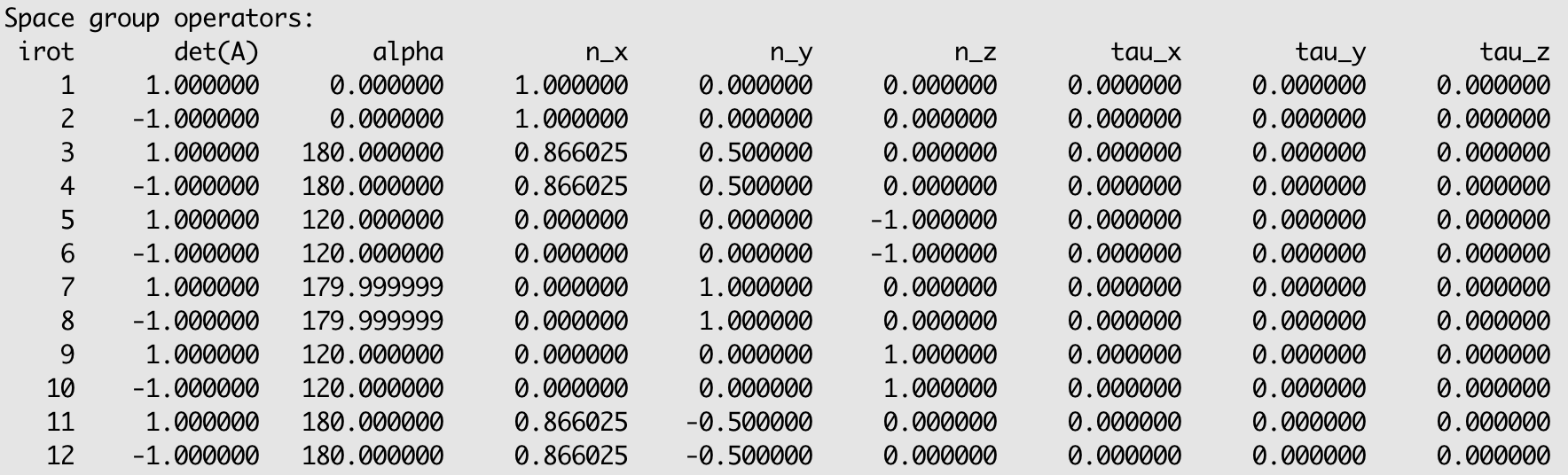
Figure 1: Screenshot of OUTCAR, showing the space group operators of Bi₂Se₃ generated by VASP.

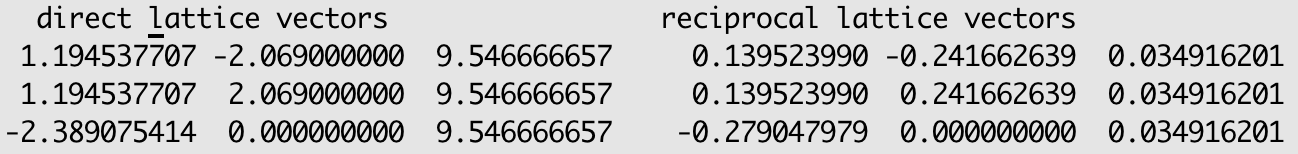
Figure 2: Screenshot of OUTCAR, showing the lattice vectors and reciprocal lattice vectors of Bi₂Se₃ which are used in VASP.

In 3D crystals, it is more convenient to use MPs in the lattices of (${\bf t}_{1},{\bf t}_{2},{\bf t}_{3}$) in real space and in reciprocal lattices of (${\bf g}_{1},{\bf g}_{2},{\bf g}_{3}$) in momentum space. They are given in the following convention:

$$\vec{v}={\bf t}_{1}v_{1}+{\bf t}_{2}v_{2}+{\bf t}_{3}v_{3}=({\bf t}_{1},{\bf t}_{2},{\bf t}_{3})\left(\begin{array}[]{c}v_{1}\\ v_{2}\\ v_{3}\end{array}\right),~{}({\bf t}_{1},{\bf t}_{2},{\bf t}_{3})\equiv\left(\begin{array}[]{ccc}t_{1x}&t_{2x}&t_{3x}\\ t_{1y}&t_{2y}&t_{3y}\\ t_{1z}&t_{2z}&t_{3z}\\ \end{array}\right);$$ (35)

$$\vec{k}=k_{1}{\bf g}_{1}+k_{2}{\bf g}_{2}+k_{3}{\bf g}_{3}=(k_{1},k_{2},k_{3})\left(\begin{array}[]{c}{\bf g}_{1}\\ {\bf g}_{2}\\ {\bf g}_{3}\end{array}\right),~{}\left(\begin{array}[]{c}{\bf g}_{1}\\ {\bf g}_{2}\\ {\bf g}_{3}\end{array}\right)\equiv\left(\begin{array}[]{ccc}g_{1x}&g_{1y}&g_{1z}\\ g_{2x}&g_{2y}&g_{2z}\\ g_{3x}&g_{3y}&g_{3z}\\ \end{array}\right).$$ (45)

$$\text{ with }\left(\begin{array}[]{c}{\bf g}_{1}\\ {\bf g}_{2}\\ {\bf g}_{3}\end{array}\right)({\bf t}_{1},{\bf t}_{2},{\bf t}_{3})=2\pi\mathbb{I}_{3\times 3}$$ (49)

The rotational symmetry operators acting on the vectors are transformed as:

$$R\vec{v}=({\bf t}_{1},{\bf t}_{2},{\bf t}_{3})Z\left(\begin{array}[]{c}v_{1}\\ v_{2}\\ v_{3}\end{array}\right),~{}R\vec{k}=(k_{1},k_{2},k_{3})Z^{-1}\left(\begin{array}[]{c}{\bf g}_{1}\\ {\bf g}_{2}\\ {\bf g}_{3}\end{array}\right);~{}$$ (56)

$$R({\bf t}_{1},{\bf t}_{2},{\bf t}_{3})=({\bf t}_{1},{\bf t}_{2},{\bf t}_{3})Z\Rightarrow Z\equiv({\bf t}_{1},{\bf t}_{2},{\bf t}_{3})^{-1}R({\bf t}_{1},{\bf t}_{2},{\bf t}_{3})$$ (57)

Thus, rotational MPs in the lattice vectors are $3\times 3$ integer matrices ($Z$), which are defined in Eq. (57). Instead of the real $R$-matrices in Cartesian coordinates in Eq. (21), the integer matrices, $Z$ and $Z^{-1}$, are actually stored and used throughout the code, which are all set in the subroutine: init.f90.

If one wants to do some sub-space-group symmetry calculations, one can modify the SGOs in OUTCAR and give the correct space group number accordingly. For example, if one only wants to know parity eigenvalues of the energy bands, one can change the list of SGOs with only two lines (i.e., identity and inversion symmetry) and give space group #2 to run irvsp.

III.3 Little group of a certain $k$-point

The eigen-wavefunctions at a certain $k$-point only support the IRs of the little group of ${\bf k}$, $LG(k)$. Therefore, for any given $k$-point, the program has to determine the ${\bf k}$-little group $LG(k)$ first. This is done in the subroutine: kgroup.f90. The $LG(k)$ are defined by Eq. (1). In the program, the integer matrices $Z^{-1}$ and Eq. (56) in momentum space are used.

III.4 Character tables for ${\bf k}$-little groups

Currently, there are two conventions of CRTs for $k$-little groups. In the first convention, the $k$ points are labeled by the IRs of the PNGs, since IRs of the space group can be expressed as IRs of the corresponding point group multiplied by a phase factor. They are suitable either for symmorphic SGs, or the inner $k$-points (not on the BZ boundary/surface) for the non-symmorphic SGs. The CRTs of PNGs are given in the Ref. Cornwell (1984); Streitwolf (1971), which have been implemented in the program irrep of the WIEN2k package Blaha et al. (2001); Persson (1999). In the second convention, all the CRTs for $k$-points of all 230 SGs are listed on the BCS Stokes et al. (2013). Therefore, the program irvsp works for all $k$-points in 230 SGs. The CRTs are retrieved from the inputs of the BCS, which is done by the subroutine: nonsymm.f90.

As an example, consider the $\Gamma$ point of Bi₂Se₃. Fig. 3 shows the CRT of the point group $D_{3d}$ in the PNG convention. Fig. 4 shows the CRT in the BCS convention. Both tables can be used to determine the IRs at $\Gamma$ in SG 166. In the table of Fig. 4, the first and two columns show the reality and the BCS labels of IRs, respectively. The following columns indicate the characters of different SGOs. The reality of an IR is given by the definition Cornwell (1984); Streitwolf (1971):

$$\frac{1}{|{\bf G}|}\sum_{j=1}^{|{\bf G}|}\chi(G_{j}^{2})=\begin{cases}\begin{array}[]{ccc}1&\text{potentially real ,}&\text{ case (a)}\\ 0&\text{essentially complex,}&\text{ case (b)}\\ -1&\text{pseudo-real ,}&\text{ case (c)}\end{array}\end{cases}$$ (58)

where $G_{j}$ is an element of the group $G$, and $|G|$ is the rank of the group $G$. In a MSG, the group $G$ is defined as the unitary part of the MSG. In case (a), the IR is equivalent to its complex representation, and also equivalent to a real representation. In case (b), the IR is not equivalent to its complex representation. In case (c), the IR is equivalent to its complex representation, but not to a real representation.

In the type-II MSGs, including pure time-reversal symmetry (TRS), the existence of anti-unitary SGOs in the $k$-little group is indicated at the beginning of the character table (Fig. 4). In the absence of SOC (integer spin), TRS doubles the degeneracy of IRs in cases (b) and (c); while in the presence of SOC (half-integer spin), it doubles the degeneracy of the IRs in cases (a) and (b).

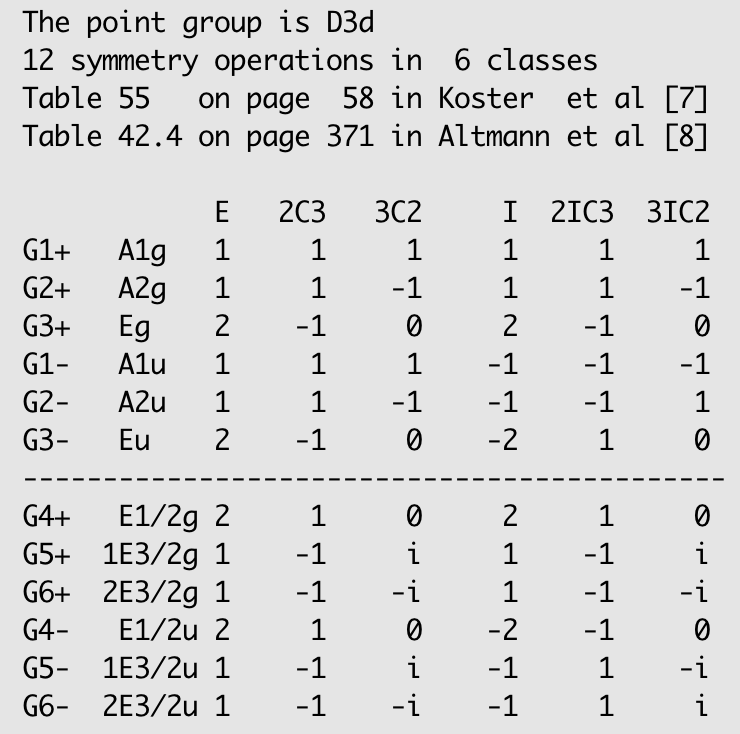
Figure 3: The character table of point group $D_{3d}$, which is used to determine the IRs (i.e., PNG convention) for the energy bands at $\Gamma$ of Bi₂Se₃ in irrep of the WIEN2k package.

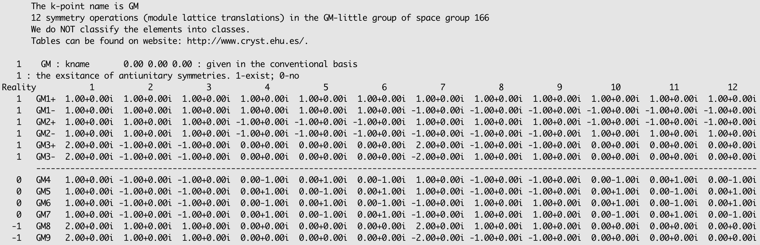
Figure 4: The character table of $\Gamma$-little group in SG 166 on the BCS, which is used to determine the IRs (i.e., BCS convention) for the energy bands at $\Gamma$ of Bi₂Se₃ in the program irvsp.

III.5 Determination of irreducible representations

After the normalization of the PW-based pseudo-wavefunctions in VASP, the traces of MPs of SGOs can be computed via Eq. (4), which are done in the subroutine chrct.f90. By comparing the obtained traces and the characters of the CRTs, the IRs can be determined (see different versions in Appendix 5).

IV Capabilities of irvsp

In the study of the properties of a material, the determination of IRs of computed electron bands is of great interest to diagnose the band crossing/anti-crossing, degeneracy and band topology. In the WIEN2k package, the program irrep classifies the IRs in PNG symmetries, which then excludes the possibility to describe certain BZ surface $k$-points for nonsymmorphic crystals. Therefore, the demand to determine the IRs for all the $k$-point in all 230 SGs is still unsatisfied. With the CRTs from the BCS, the program – irvsp – is developed to meet this demand with the interface to the VASP package. The associated library – irrep_bcs.a – can be easily linked to by other ab-initio packages. The obtained IRs are labeled in the convention of the BCS notation, which can be directly compared with the elementary band representations (EBRs) of the TQC theory, to further check the topology of a set of bands in materials.

V Installation and usage

In this section, we will show how to install and use the irvsp software package. This program is an open source free software package. It is released on Github under the GNU Lesser General Public License, https://www.gnu.org/licenses/lgpl-3.0.html, and it can be downloaded directly from the public code archive: https://github.com/zjwang11/irvsp/blob/master/src_irvsp_v2.tar.gz.

To build and install irvsp, only a Fortran 90 compiler is needed. The downloaded irvsp software package is likely a compressed file with a zip or tar.gz suffix. One should uncompress it first, then move into the src_irvsp_v2 folder. After setting up the Fortran compiler in the Makefile file, the executable binary irvsp can be compiled by typing the following command in the current directory (src_irvsp_v2):

⬇

$ ./configure.sh

$ source ~/.bashrc

$ make

Before running irvsp, the user must provide two consistent files: WAVECAR and OUTCAR. The two files are generated by the VASP package in fixed format. It is designed to be simple and user friendly. After a running of VASP with WAVECAR and OUTCAR output, the program irvsp can be run immediately. Giving a correct space group number ($sgn~{}\in~{}[1,230]$) and a set of energy bands (from the $m$th band to the $n$th band), the program can be executed by the following command:

⬇

$ irvsp -sg $sgn [-nb $m $n] > outir &

VI Examples

Very recently, the codes vasp2trace and CheckTopologicalMat have been designed for TQC in the Ref. Vergniory et al. (2019). However, they are not suitable for non-maximal HSK points. In fact, vasp2trace is extracted from irvsp to interface with CheckTopologicalMat. Here, we take topological materials PdSb₂ and Bi as examples to show how to study topological properties of new materials with irvsp. The necessary files for these materials are given as the examples in the archive src_irvsp_v2.tar.gz .

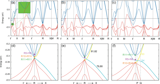
Figure 5: Electronic band structures of PdSb₂ without strain (a), with 0.31% (b) and 0.62% (c) tensile strains. Panels (d-f) are the zoom-in plots of panels (a-c) near the R point. In our calculations, the total number of electrons is 80. The different IRs at R are labeled by green triangles (R11+R11), orange squares (R10+R10) and purple circles (R5+R6). The two crossing bands along R--X belong to S3 (yellow) and S4 (cyan), respectively. P $[0.4912~{}(\frac{2\pi}{a}),0.5000~{}(\frac{2\pi}{a}),0.4912~{}(\frac{2\pi}{a})]$ and Q $[0.4722~{}(\frac{2\pi}{a}),0.5000~{}(\frac{2\pi}{a}),0.4722~{}(\frac{2\pi}{a})]$ are two points near the crossing point on the R--X line.

VI.1 PdSb₂

PdSb₂ was predicted to be a candidate hosting sixfold-degenerate fermions because of nonsymmorphic symmetry Bradlyn et al. (2016); Chapai et al. (2019). The crystal of PdSb₂ is a cubic structure of SG 205. We adopt the experimental lattice constant $a$ Pratt et al. (1968); Furuseth et al. (1965); Brese and von Schnering (1994) and fully relax the coordinates of inner atomic positions. In the obtained band structure (BS) along the high-symmetry lines (Fig. 5(a)), we note that there is a tiny gap ($\sim 10$ meV) between two sixfold degeneracies at R. Then, we want to know the corresponding IRs of two sixfold degeneracies and how they are going to evolve under strains. For this purpose, we performed the calculations with different tensile strains (i.e., $\Delta a/a=0.31$% and $\Delta a/a=0.62$%). Their electronic band structures are shown in Figs. 5 (b) and (c), respectively. Comparing with the strain-free BS in Fig. 5(a), we find that the overall BS doesn’t change very much, except for the R point. The zoom-in plots around R are shown in lower panels of Fig. 5. The R point is a $k$-point with nonsymmorphic symmetry in SG 205, where IRs of the space group can not be expressed as IRs of the corresponding point group multiplied by a phase factor. By running irvsp, the IRs at R are obtained. Figs. 6 (a-c) show the results of IRs for the low-energy bands. The number of total electrons is 80 for PdSb₂. It is shown that the energy ordering of electron bands is changed at $R$ under tiny strains.

The IRs at all the maximal HSK points can be computed directly by irvsp. The trace file -- trace.txt will be generated if only maximal HSK points are given in KPOINTS. By directly comparing these obtained IRs with the EBRs of the TQC theory (released on the BCS) and solving the compatibility relations, we can find that it is a topological insulating phase without strain, while it’s a symmetry-enforced semimetallic phase with tiny tensile strains.

To further obtain the crossing points in the system, we computed the IRs along the R--X line (named S [$u,0.5,u$] in units of $\frac{2\pi}{a}$). These points are also non-symmorphic, which are on the boundary of the 3D BZ for SG 205. The CRT for the S point is listed in Fig. S2. For the P and Q points in Fig. 5(f) of the strained crystal, we show the results of obtained IRs in Fig. 7. At the P point, the 79-80 degenerate bands are assigned to ‘‘S3+S3", while 81-82 degenerate bands are assigned to ‘‘S4+S4". However, at the Q point, the results are in the opposite way. Without doing further calculations with a denser kmesh between P and Q points, we can still conclude that it’s a real 4-fold crossing along R--X on the BZ boundary, which is robust against SOC. The double degeneracy is due to the presence of TRS. The symmetry #15 is the operator $g_{y}\equiv\{M_{y}|0\frac{1}{2}\frac{1}{2}\}$. Therefore, the doubly-degenerate bands have the same $g_{y}$ eigenvalue ($\{S3,S3\}$ or $\{S4,S4\}$), and the 4-fold crossing point along R--X is protected by $g_{y}$ symmetry. As a result, the crossing 4-fold points actually form a Dirac nodal ring on the BZ boundary. Considering the full symmetry of SG 205, we conclude that there are three Dirac nodal rings in PdSb₂ with tiny strains, which can be further checked in experiments in the future.

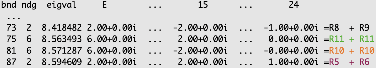
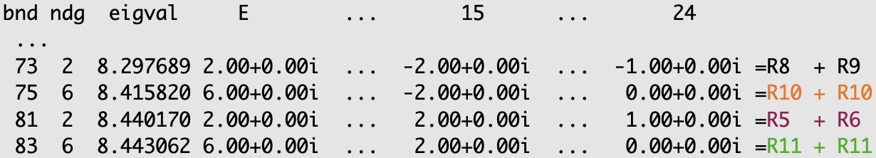
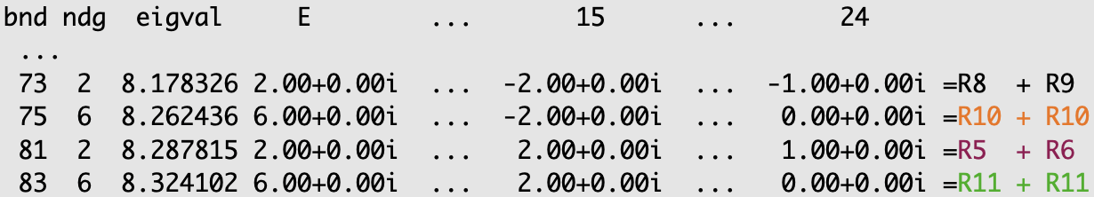
Figure 6: The IRs at R are determined by the program irvsp. The CRT of the R-little group is shown in Fig. S1 in Appendix 4. The first three columns stand for the band indices, degeneracies, and the energies (without subtracting the Fermi energy E_F). The following columns indicate the traces (characters) of the corresponding space group operators (listed as ‘‘E, 2, $\dots$, 24"). The assigned IR labels are output to the right of the equality sign ‘‘=". The (a), (b), (c) panels are the obtained results for the three crystal structures, respectively.

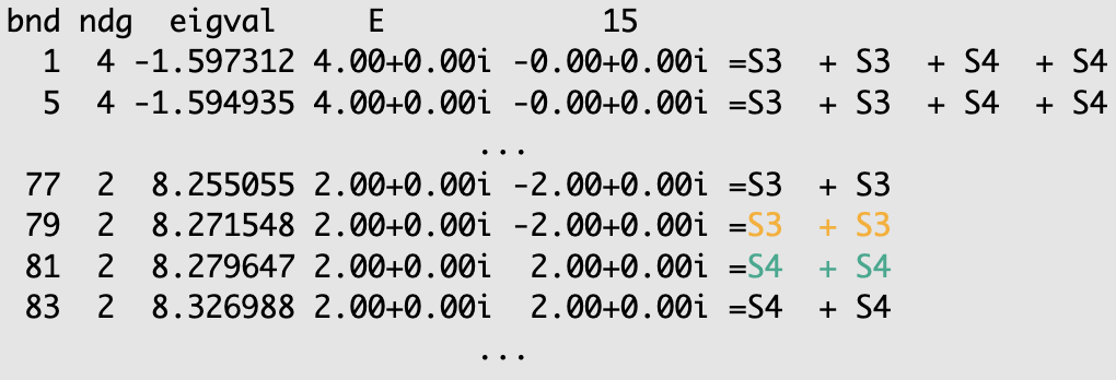
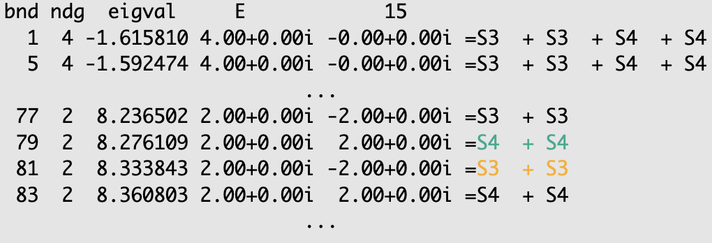
Figure 7: The IRs are obtained by irvsp for P (a) and Q (b) as depicted in Fig. 5(f).

centerlast HSK six valence bands GM GM8 (2); GM8 (2); GM4 GM5 (2); [6] T T9 (2); T8 (2); T6 T7 (2); [6] F F3 F4 (2); F5 F6 (2); F5 F6 (2); [6] L L3 L4 (2); L5 L6 (2); L5 L6 (2); [6]

Table 2: The IRs at maximal HSK points obtained by irvsp for Bismuth. ‘‘($p$)" indicates the degeneracy of the bands, while ‘‘[$q$]" indicates the total number of the computed bands at the $k$-point.

VI.2 Bismuth

As aforementioned, with the IRs at maximal HSK points obtained by irvsp, we can further check the topology by comparing them with the EBRs of the TQC theory. Here, we will take Bi as an example to briefly introduce the process. The element Bismuth has the rhombohedral structure of SG 166. The maximum HSK points of SG 166 are listed on the BCS, as $\Gamma$(GM), T, F, L. After performing the ab-initio calculations to obtain the eigen-wavefunctions at maximal HSK points, the obtained IRs of the occupied bands are given in Table 2. From the TQC and BCS, the EBRs of SG 166 are obtained, as shown in Fig. 8. As there are only six valence bands, we can find that they do not belong to any EBR induced from the $9d$ or $9e$ Wyckoff position. In the EBRs induced from the $3a$ and $3b$ Wyckoff positions, we can find that the number of the pairs of F5F6 at F has to be the same as the total number of the IRs GM9 and GM6GM7 at $\Gamma$. In Bismuth, the obtained IRs have three IRs of F5F6, but neither GM9 nor GM6GM7. Therefore, the occupied bands of Bisumth can not be expressed as any sum of EBRs in SG 166. In other words, it has to be topological Schindler et al. (2018).

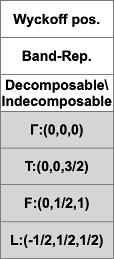
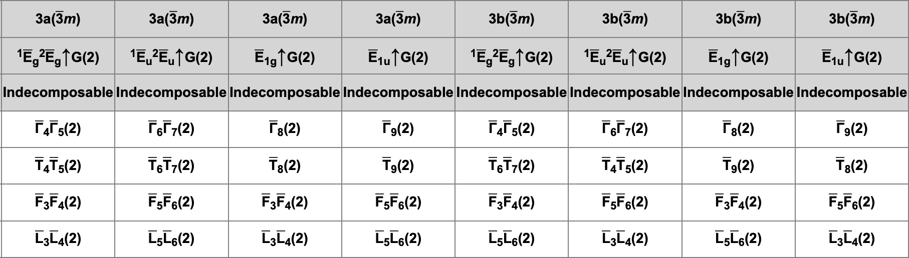
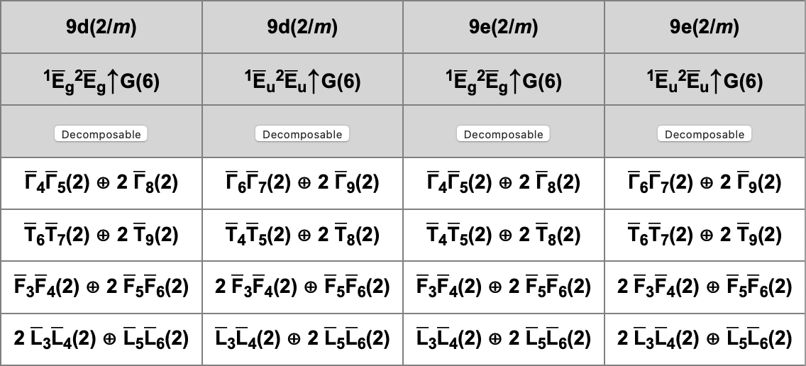
Figure 8: A complete list of the EBRs of space group 166 in the presence of SOC. Each EBR is defined by a Maximal Wyckoff site ($n$x) and an IR of its site-symmetry group, which are indicated by the first and second rows, respectively. Then, the following rows present the IRs at the Maximal HSK points.

VII Conclusions

In summary, we present an open-source software package -- irvsp -- that determines the IRs of electronics states in the VASP. It is very user-friendly and is written in Fortran 90/77, showing a powerful function to analyze the IRs for all the $k$-points in all 230 SGs, including nonsymmorphic crystals. The associated library -- irrep_bcs.a -- can be interfaced with other DFT packages. We show how to use it to identify IRs and further get the topological property for a new material. As an example, we explore a topological material PdSb₂, whose topology is very sensitive to the lattice parameter. Under tiny strains, it is identified as a four-fold Dirac nodal-line metal.

Acknowledgments We thank Dr. Peter Blaha and Dr. Luis Elcoro for sharing the character tables of 32 point groups implemented in the WIEN2k package and the character tables of 230 SGs for all $k$-points on the BCS. This work was supported by the National Nature Science Foundation of China (Grant No. 11974395), the Strategic Priority Research Program of Chinese Academy of Sciences (Grant No. XDB33000000), the Center for Materials Genome and the CAS Pioneer Hundred Talents Program. Q. S. W. acknowledges the support of NCCR MARVEL.

APPENDIX

1 tbbox.in for Bi₂Se₃

case = soc ! lda or soc

proj:
orbt = 2
ntau = 5
0.39900000 0.39900000 0.39900000 1 3 ! x1, x2, x3, itau, iorbit
0.60100000 0.60100000 0.60100000 1 3
0.20600000 0.20600000 0.20600000 2 3
0.79400000 0.79400000 0.79400000 2 3
0.00000000 0.00000000 0.00000000 2 3
end projections

kpoint:
kmesh = 10
Nk = 4
0.00000000 0.00000000 0.00000000 ! k1: y1,y2,y3
0.50000000 0.50000000 0.50000000 ! k2
0.50000000 0.50000000 0.00000000 ! k3
0.00000000 0.50000000 0.00000000 ! k4
end kpoint_path

unit_cell:
1. 194537707 -2. 069000000 9. 546666657 0. 139523990 -0. 241662639 0. 034916201 1. 194537707 2. 069000000 9. 546666657 0. 139523990 0. 241662639 0. 034916201 -2. 389075414 0. 000000000 9. 546666657 -0. 279047979 0. 000000000 0. 034916201 1 1. 000000 0. 000000 1. 000000 0. 000000 0. 000000 0. 000000 0. 000000 0. 000000 2 -1. 000000 0. 000000 1. 000000 0. 000000 0. 000000 0. 000000 0. 000000 0. 000000 3 1. 000000 180. 000000 0. 866025 0. 500000 0. 000000 0. 000000 0. 000000 0. 000000 4 -1. 000000 180. 000000 0. 866025 0. 500000 0. 000000 0. 000000 0. 000000 0. 000000 5 1. 000000 120. 000000 0. 000000 0. 000000 -1. 000000 0. 000000 0. 000000 0. 000000 6 -1. 000000 120. 000000 0. 000000 0. 000000 -1. 000000 0. 000000 0. 000000 0. 000000 7 1. 000000 179. 999999 0. 000000 1. 000000 0. 000000 0. 000000 0. 000000 0. 000000 8 -1. 000000 179. 999999 0. 000000 1. 000000 0. 000000 0. 000000 0. 000000 0. 000000 9 1. 000000 120. 000000 0. 000000 0. 000000 1. 000000 0. 000000 0. 000000 0. 000000 10 -1. 000000 120. 000000 0. 000000 0. 000000 1. 000000 0. 000000 0. 000000 0. 000000 11 1. 000000 180. 000000 0. 866025 -0. 500000 0. 000000 0. 000000 0. 000000 0. 000000 12 -1. 000000 180. 000000 0. 866025 -0. 500000 0. 000000 0. 000000 0. 000000 0. 000000
end unit_cell

centerlast PNG BCS PW basis src_irvsp_v1.tar.gz src_irvsp_v2.tar.gz TB basis src_ir2tb_v1.tar.gz src_ir2tb_v2.tar.gz

Table S1: Besides the src_irvsp_v2.tar.gz code mainly discussed in the main text, there are more codes developed, which are available in the repository: https://github.com/zjwang11/irvsp/. Different versions of the codes are developed based on the different types of the WFs and conventions of the CRTs.

2 The brief description of ir2tb

Based on the different types of the WFs and conventions of the CRTs, different versions of the codes are developed, as shown in Table S1. The program ir2tb is based on the TB WFs. BLAS and LAPACK linear algebra libraries are needed to diagonalize the TB Hamiltonian. To compile ir2tb, one needs to copy the library irrep_bcs.a to the folder src_ir2tb_v2 and type the following command:

⬇

$ make

The program ir2tb needs two input files: tbbox.in and case_hr.dat. The case_hr.dat file, containing the TB parameters in Wannier90 format Marzari et al. (2012), may be generated by the software Wannier90 Mostofi et al. (2014) with symmetrization Gresch et al. (2018), or generated by users with a toy TB model, or generated from Slater-Koster method Slater and Koster (1954) or a discretization of $k\cdot p$ model onto a lattice Willatzen and Voon (2009).

The tbbox.in file provides detailed information about the TB Hamiltonian (i.e., the case_hr.dat file), which is summarized in Table S2. It is an essential input for the program ir2tb. The tag case = lda (case = soc) indicates that the TB Hamiltonian does not (does) have the SOC effect. The lda/soc_hr.dat is needed accordingly. In the proj block, orbt = 1 or 2 indicates the convention of the local orbital ordering on each atom. The local orbitals in convention 1 are listed in Table S3, while those in convention 2 are in the order as implemented in Wannier90. ntau indicates the total number of the atoms in the TB Hamiltonian, which also means how many lines follow in this block. The local orbitals of the TB Hamiltonian are provided by : x1,x2,x3, itau, iorbit. x1,x2,x3 stand for the positions of atoms: $\tau_{i}=(x_{1}{\bf t}_{1},x_{2}{\bf t}_{2},x_{3}{\bf t}_{3})$; itau stand for the kinds of atoms; and iorbit stand for the total numbers of local orbitals on different atoms. So far, iorbit is limited to the values of {1,3,5,4,6,7,8,9}, whose detailed orbital informations are provided in Table S3. In the case of case = soc, the local orbitals will be doubled automatically: the first half are spin-up and the second half are spin-down. In the kpoint block, the $k$-path is given as $k_{1}$ -- $k_{2}$ -- $\dots$ -- $k_{N}$ with kmesh points on each segment. The unit_cell block gives the lattice vectors and reciprocal lattice vectors in first three lines, followed by space group operators, which are the same lines as irvsp reads in OUTCAR file.

centerlast Comments Descriptions ! lda or soc lda: nspin=1 (without SOC); soc: nspin=2 (with SOC) ! x1,x2,x3,itau,iorbit defining $\tau_{i}=(x_{1}{\bf t}_{1},x_{2}{\bf t}_{2},x_{3}{\bf t}_{3})$, iorbit $\in~{}\{1,3,4,5,6,7,8,9\}$ ! k1: y1,y2,y3 defining ${\bf k}_{1}=(y_{1}{\bf g}_{1},y_{2}{\bf g}_{2},y_{3}{\bf g}_{3})$; kpath is along ${\bf k}_{1}-{\bf k}_{2}-\dots-{\bf k}_{N}$. ! b1x b1y b1z; g1x g1y g1z defining ${\bf t}_{1}=(b_{1x}\hat{x},b_{1y}\hat{y},b_{1z}\hat{z})$; ${\bf g}_{1}=2\pi(g_{1x}\hat{x},g_{1y}\hat{y},g_{1z}\hat{z})$ ! SN,Det,omega,nx,ny,nz,v1,v2,v3 defining ${\cal O}_{s}=\{R_{s}|{\bf v}_{s}\}$ with $R_{s}=Det\cdot e^{-i\omega(\vec{n}\cdot\vec{L})}$ and ${\bf v}_{s}=(v_{1}{\bf t}_{1},v_{2}{\bf t}_{2},v_{3}{\bf t}_{3})$. SN stands for the sequential number.

Table S2: A brief summary of tbbox.in.

centerlast iorbit local orbitals $D$-matrices in Eq. (7) 1 $s$ $D^{1}=1$ 3 $p_{x},p_{y},p_{z}$ $D^{3}=Det\cdot e^{-i\omega(\vec{n}\cdot\vec{L})}$ 5 $d_{xy},d_{yz},d_{zx},d_{x^{2}-y^{2}},d_{3z^{2}-r^{2}}$ $D^{5}=e^{-i\omega(\vec{n}\cdot\vec{P})}$ 4 $s,p_{x},p_{y},p_{z}$ $D^{4}=D^{1}\oplus D^{3}$ 6 $s,d_{xy},d_{yz},d_{zx},d_{x^{2}-y^{2}},d_{3z^{2}-r^{2}}$ $D^{6}=D^{1}\oplus D^{5}$ 8 $p_{x},p_{y},p_{z},d_{xy},d_{yz},d_{zx},d_{x^{2}-y^{2}},d_{3z^{2}-r^{2}}$ $D^{8}=D^{3}\oplus D^{5}$ 9 $s,p_{x},p_{y},p_{z},d_{xy},d_{yz},d_{zx},d_{x^{2}-y^{2}},d_{3z^{2}-r^{2}}$ $D^{9}=D^{1}\oplus D^{3}\oplus D^{5}$ 7 $f_{xyz},f_{5x^{3}-xr^{2}},f_{5y^{3}-yr^{2}},f_{5z^{3}-zr^{2}},f_{x(y^{2}-z^{2})},f_{y(z^{2}-r^{2})},f_{z(x^{2}-y^{2})}$ $D^{7}=Det\cdot e^{-i\omega(\vec{n}\cdot\vec{F})}$

Table S3: The local orbitals in convention 1 (i.e., orbt = 1) are given below. The vector $\vec{L}$ is given in Eq. (21) in the main text, while the vectors $\vec{P}$ and $\vec{F}$ are given in Eqs. (59--62) in Appendix 2.

$$P_{x}=\left(\begin{array}[]{ccccc}0&0&-i&0&0\\ 0&0&0&-i&-i\sqrt{3}\\ i&0&0&0&0\\ 0&i&0&0&0\\ 0&i\sqrt{3}&0&0&0\\ \end{array}\right);P_{y}=\left(\begin{array}[]{ccccc}0&i&0&0&0\\ -i&0&0&0&0\\ 0&0&0&-i&i\sqrt{3}\\ 0&0&i&0&0\\ 0&0&-i\sqrt{3}&0&0\\ \end{array}\right);P_{z}=\left(\begin{array}[]{ccccc}0&0&0&2i&0\\ 0&0&i&0&0\\ 0&-i&0&0&0\\ -2i&0&0&0&0\\ 0&0&0&0&0\\ \end{array}\right)$$ (59)

$$F_{x}=\left(\begin{array}[]{ccccccc}0&0&0&0&2i&0&0\\ 0&0&0&0&0&0&0\\ 0&0&0&\frac{3i}{2}&0&0&\frac{i\sqrt{15}}{2}\\ 0&0&-\frac{3i}{2}&0&0&\frac{i\sqrt{15}}{2}&0\\ -2i&0&0&0&0&0&0\\ 0&0&0&-\frac{i\sqrt{15}}{2}&0&0&-\frac{i}{2}\\ 0&0&-\frac{i\sqrt{15}}{2}&0&0&\frac{i}{2}&0\\ \end{array}\right)$$ (60)

$$F_{y}=\left(\begin{array}[]{ccccccc}0&0&0&0&0&2i&0\\ 0&0&0&-\frac{3i}{2}&0&0&\frac{i\sqrt{15}}{2}\\ 0&0&0&0&0&0&0\\ 0&\frac{3i}{2}&0&0&\frac{i\sqrt{15}}{2}&0&0\\ 0&0&0&-\frac{i\sqrt{15}}{2}&0&0&\frac{i}{2}\\ -2i&0&0&0&0&0&0\\ 0&-\frac{i\sqrt{15}}{2}&0&0&-\frac{i}{2}&0&0\\ \end{array}\right)$$ (61)

$$F_{z}=\left(\begin{array}[]{ccccccc}0&0&0&0&0&0&2i\\ 0&0&\frac{3i}{2}&0&0&\frac{i\sqrt{15}}{2}&0\\ 0&-\frac{3i}{2}&0&0&\frac{i\sqrt{15}}{2}&0&0\\ 0&0&0&0&0&0&0\\ 0&0&-\frac{i\sqrt{15}}{2}&0&0&-\frac{i}{2}&0\\ 0&-\frac{i\sqrt{15}}{2}&0&0&\frac{i}{2}&0&0\\ -2i&0&0&0&0&0&0\\ \end{array}\right)$$ (62)

3 The standard settings for POSCAR and maximal HSK points

The standard (default) settings of POSCAR are listed as follows:

• unique axis b (cell choice 1) for SGs within the monoclinic system.

• obverse triple hexagonal unit cell for R SGs.

• the origin choice two - inversion center at (0,0,0) - for the centrosymmetric SGs.

Before one is actually doing the VASP calculations, we strongly suggest that one could run the phonopy program to get the space group number and standardise the POSCAR with the following command:

⬇

$ phonopy --tolerance 0.01 --symmetry -c POSCAR

$ cp PPOSCAR POSCAR

The maximal HSK points from the BCS are given in the conventional reciprocal lattice vectors, while the lattice vectors in VASP usually are given in the primitive cell. The transformation depends on the type of the lattice. There are only seven different types of lattices, i.e. $P,C,B,A,R,F$ and $I$. In the $X$ type, the primitive lattices ($\vec{p}_{1}$, $\vec{p}_{2}$, $\vec{p}_{3}$) are defined by a transformation matrix $M_{X}$.

$$\left(\begin{array}[]{ccc}\vec{p}_{1}&\vec{p}_{2}&\vec{p}_{3}\end{array}\right) = \left(\begin{array}[]{ccc}\vec{c}_{1}&\vec{c}_{2}&\vec{c}_{3}\end{array}\right)\cdot M_{X}$$ (65)

where $\vec{c}_{1}$, $\vec{c}_{2}$ and $\vec{c}_{3}$ are the standard conventional lattices. In the program, all the matrices $M_{X}$ are given as follows:

$$M_{P}=\left(\begin{array}[]{ccc}1&0&0\\ 0&1&0\\ 0&0&1\end{array}\right);~{}M_{C}=\left(\begin{array}[]{ccc}0.5&0.5&0\\ -0.5&0.5&0\\ 0&0&1\end{array}\right);~{}M_{B}=\left(\begin{array}[]{ccc}0.5&0&-0.5\\ 0&1&0\\ 0.5&0&0.5\end{array}\right);~{}M_{A}=\left(\begin{array}[]{ccc}1&0&0\\ 0&0.5&-0.5\\ 0&0.5&0.5\end{array}\right);~{}$$

$$M_{R}=\left(\begin{array}[]{ccc}2/3&-1/3&-1/3\\ 1/3&1/3&-2/3\\ 1/3&1/3&1/3\end{array}\right);~{}M_{F}=\left(\begin{array}[]{ccc}0&0.5&0.5\\ 0.5&0&0.5\\ 0.5&0.5&0\end{array}\right);~{}\\ M_{I}=\left(\begin{array}[]{ccc}-0.5&0.5&0.5\\ 0.5&-0.5&0.5\\ 0.5&0.5&-0.5\end{array}\right).$$

4 The character tables for R-little group and S-little group

Figs. S1 and S2 show the character tables for R-little group and S-little group, respectively. At the $k$-point [$(u,v,w)$ given in the conventional reciprocal basis], the block $\begin{array}[]{c}x+iy\\ a~{}b~{}c\end{array}$ in Fig. S2 corresponds to a complex value of $(x+iy)\cdot exp[i\pi(au+bv+cw)]$.

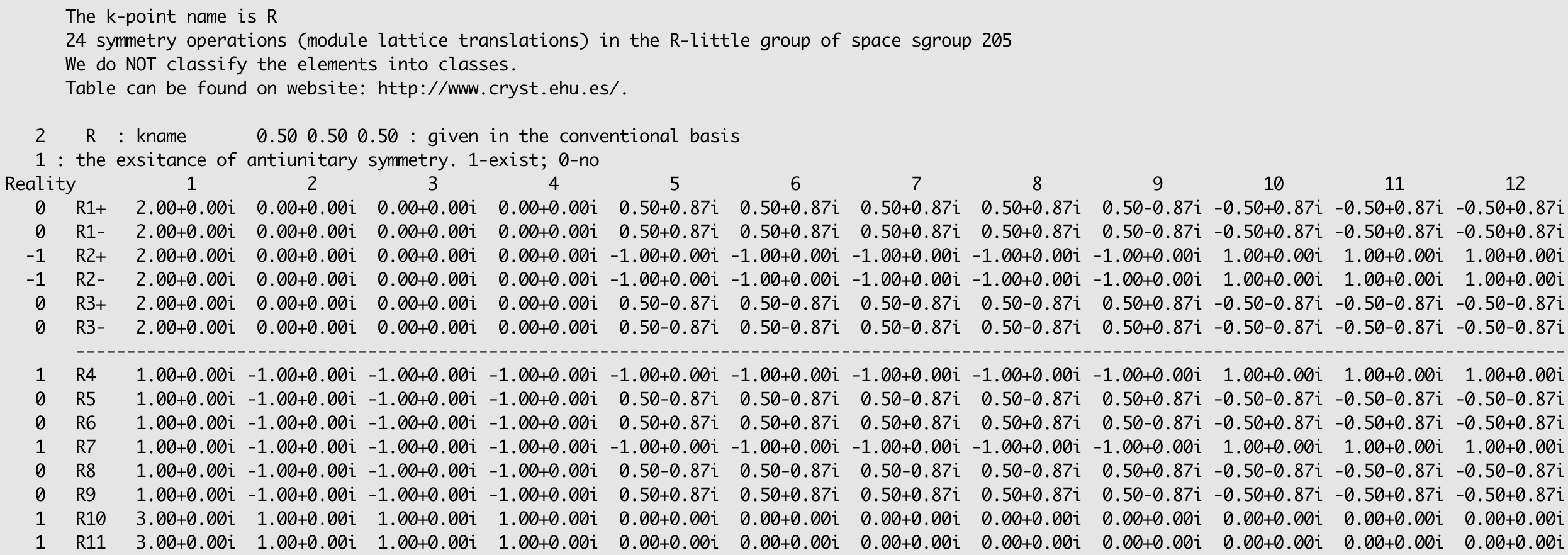
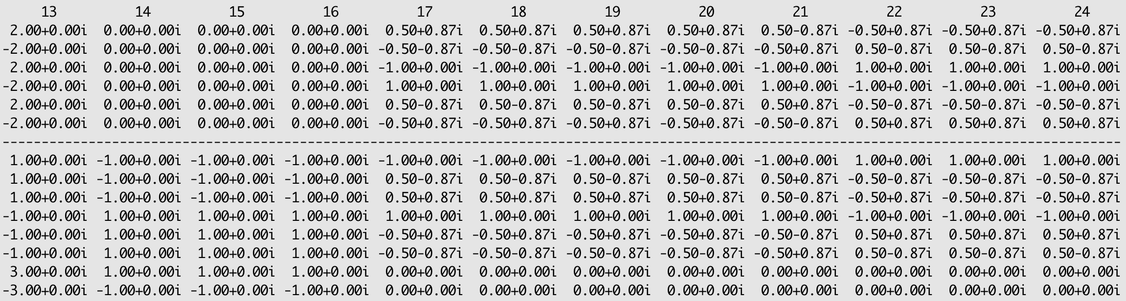
Figure S1: The CRT of R-little group in the BCS convention.

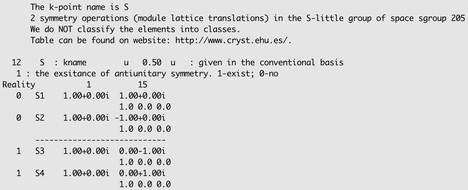
Figure S2: The CRT of S-little group in the BCS convention.

5 Other versions of irvsp

Four versions of irvsp are implemented, as shown in Table S4. Version I works similarly as irrep in the WIEN2k package and presents the IRs with PNG symmetries. This version can thus not classify the special $k$-points on the boundary of the Brillouin zone of nonsymmorphic crystals, that is, when $exp[-ik(R_{s}{\bf v}_{t}+{\bf v}_{s})]\neq 1$ for some $O_{s}$ and $O_{t}$ in LG(k). Version II works for those $k$-points for nonsymmorphic SGs, where version I doesn’t work. Version III combines version I and II. In the (default) version IV, it works for all the $k$-points and all 230 SGs in the convention of the BCS notaion. One can use an optional flag -v to execute other versions of irvsp.

⬇

$ irvsp -sg $sgn [-v $nv] [-nb $m $n] > outir &

centerlast Version CRTs Brief description version I PNG It resembles an analogue of the program irrep in the WIEN2k package. version II BCS It works only for the $k$-points, where version I does not work. version III PNG&BCS It combines version I and version II. version IV      (default) BCS It works for all the $k$-points and all 230 SGs, including nonsymmorphic SGs. All the IRs are labeled in the convention of the BCS notation.

Table S4: Four versions of irvsp are implemented. The first column indicates the version number, the second column shows the convention of reference CRTs, and the brief description is followed in the last column.

6 The library -- irrep_bcs.a

The library irrep_bcs.a is developed to be interfaced with other DFT packages. Calling the main subroutine irrep_bcs can output the IRs labeled in the convention of BCS notation. The program ir2tb is an example of calling the library mode. In other words, ir2tb has to be compiled by linking to the library irrep_bcs.a. The source files of the library irrep_bcs.a are released in the public archive: https://github.com/zjwang11/irvsp/blob/master/lib_irrep_bcs.tar.gz

To compile the library, one should first uncompress the archive lib_irrep_bcs.tar.gz, then move into the folder lib_irrep_bcs and type the following command:

⬇

$ ./configure.sh

$ source ~/.bashrc

$ make lib

The first two commands add an environment variable IRVSPDATA and the third command create the library irrep_bcs.a in the current folder. There are three main subroutines: irrep_bcs, pw_setup, tb_setup in the library. Their headers and detailed descriptions are given below (dp = 8).

⬇

subroutine irrep_bcs(sgn, num_sym, &

rot_input, tau_input, SO3_input, SU2_input, &

KKK, WK, kphase, &

num_bands, m, n, ene_bands, &

spinor, dim_basis, num_basis, &

coeffa, coeffb, &

Gphase_pw, rot_vec_pw, rot_mat_tb)

• integer, intent(in) :: sgn
  The space group number.

• integer, intent(in) :: num_sym
  The number of space-group operations $\mathcal{O}_{s}\equiv\{R_{s}|{\bf v}_{s}\}$ (module the integer lattice translations).

• integer, dimension(3,3,num_sym), intent(in) :: rot_input
  The rotation part $R_{s}$ of space-group operations $\mathcal{O}_{s}$ with respect to primitive lattice vectors [i.e., the matrix $Z$ in Eq. (57)].

• real(dp), dimension(3,num_sym), intent(in) :: tau_input
  The translation part ${\bf v}_{s}$ of space-group operations $\mathcal{O}_{s}$ with respect to primitive lattice vectors.

• real(dp), dimension(3,3,num_sym), intent(in) :: SO3_input
  The $R_{s}$ given in Cartesian coordinates [i.e., $R(\omega,\vec{n})$ in Eq. (21)].

• complex(dp), dimension(2,2,num_sym), intent(in) :: SU2_input
  The $R_{s}$ given in spin-1/2 space [i.e., $S(\omega,\vec{n})$ in Eq. (28)].

• integer, intent(in) :: KKK
  The sequential number of the given k-point.

• real(dp), dimension(3), intent(in) :: WK
  The coordinates of the k-point with respect to primitive reciprocal lattice vectors.

• complex(dp), dimension(num_sym), intent(in) :: kphase
  The k-dependent phase factors due to the translation part ${\bf v}_{s}$ [i.e., $e^{-i{\bf k}\cdot{\bf v}_{s}}$ in Eq. (4) or $e^{-i(R_{s}{\bf k}\cdot{\bf v}_{s})}$ in Eq. (9)].

• integer, intent(in) :: num_bands
  The total number of bands.

• integer, intent(in) :: m, n
  The IRs of the set of bands [m, n] are computed.

• real(dp), dimension(num_bands), intent(in) :: ene_band
  The energy of the bands at the k-point.

• logical, intent(in) :: spinor
  Set to .true. if underlying electronic structure calculation has been performed with spinor wavefunctions.

• integer, intent(in) :: dim_basis
  The reserved number of the PW/TB basis.
  If rot_vec_pw is given, dim_basis >= num_basis for any k-point.
  If rot_mat_tb is given, one should set dim_basis = num_basis.

• integer, intent(in) :: num_basis
  The number of PW or orthogonal TB basis for the given k-point (note: the number of PWs for different k-points are usually different).

• complex(dp), dimension(dim_basis,num_bands),intent(in) :: coeffa
  The coefficients of spin-up part of wave functions at the given k-point (note: only coeffup_basis(1:num_basis, 1:num_bands) is nonzero).

• complex(dp), dimension(dim_basis,num_bands),intent(in) :: coeffb
  The coefficients of spin-down part of wave functions at the given k-point if spinor is .true. (note: only coeffdn_basis(1:num_basis, 1:num_bands) is nonzero).

• complex(dp), dimension(dim_basis,num_bands),intent(in), optional :: Gphase_pw
  The phase factors dependent on the PW vectors [i.e., $e^{-i{\bf G}_{j^{\prime}}\cdot{\bf v}_{s}}$ in Eq. (4)].

• integer(dp), dimension(dim_basis,num_bands),intent(in), optional :: rot_vec_pw
  The transformation vectors of space-group operations $\mathcal{O}_{s}$, which send the $j$th PW to the $j^{\prime}$th PW [i.e., ${\bf G}_{j^{\prime}}\equiv R_{s}({\bf k}+{\bf G}_{j})-{\bf k}$ in Eq. (4)].

• integer(dp), dimension(dim_basis,dim_basis,num_bands),intent(in), optional :: rot_mat_tb
  The transformation matrices of space-group operations $\mathcal{O}_{s}$ in the orthogonal TB basis [i.e., $\overline{V(R_{s}{\bf k}-{\bf k})D}$ in Eq. (9)].

⬇

subroutine pw_setup(WK, lattice, &

num_sym, det, angle, axis, tau, &

dim_basis, num_basis, Gvec, &

rot, SO3, SU2, &

kphase, Gphase_pw, rot_vec_pw)

• real(dp), dimension(3), intent(in) :: WK
  The coordinates of the k-point with respect to primitive reciprocal lattice vectors.

• real(dp), dimension(3,3), intent(in) :: lattice(3,3)
  The primitive lattice vectors in Cartesian coordinates [i.e., $({\bf t_{1}},{\bf t_{2}},{\bf t_{3}})$ in Eq. (35)].

• integer, intent(in) :: num_sym
  The number of space-group operations $\mathcal{O}_{s}\equiv\{R_{s}|{\bf v}_{s}\}$ (module the integer lattice translations).

• real(dp), dimension(num_sym), intent(in) :: det
  The determination of the rotation part $R_{s}$ of space-group operations $\mathcal{O}_{s}$ [i.e., $Det$ in Eq. (21)].

• real(dp), dimension(num_sym), intent(in) :: angle
  The rotation angle of space-group operations $\mathcal{O}_{s}$ [i.e., $\omega$ in Eq. (21)].

• real(dp), dimension(3,num_sym), intent(in) :: axis
  The rotation axis of space-group operations $\mathcal{O}_{s}$ in Cartesain coordinates[i.e., $\vec{n}$ in Eq. (21)].

• real(dp), dimension(3,num_sym), intent(in) :: tau
  The translation part ${\bf v}_{s}$ of space-group operations $\mathcal{O}_{s}$ with respect to primitive lattice vectors.

• integer, intent(in) :: dim_basis
  The reserved number of the PW basis (dim_basis >= num_basis).

• integer, intent(in) :: num_basis
  The number of the PWs for the given k-point (note: num_basis for different k-points are usually different).

• integer, dimension(3, dim_basis), intent(in) :: Gvec
  The plane-wave G-vector with respect to reciprocal lattice vectors [i.e., ${\bf G}_{j}$ in Eq. (3)].

• integer, dimension(3,3,num_sym), intent(out) :: rot
  The rotation part $R_{s}$ of $\mathcal{O}_{s}$ with respect to primitive lattice vectors [i.e., the matrix $Z$ in Eq. (57)].

• real(dp), dimension(3,3,num_sym), intent(out) :: SO3
  The $R_{s}$ given in Cartesian coordinates [i.e., $R(\omega,\vec{n})$ in Eq. (21)].

• complex(dp), dimension(2,2,num_sym), intent(out) :: SU2
  The $R_{s}$ given in spin-1/2 space [i.e., $S(\omega,\vec{n})$ in Eq. (28)].

• complex(dp), dimension(num_sym), intent(out) :: kphase
  The k-dependent phase factors due to the translation part ${\bf v}_{s}$ [i.e., $e^{-i{\bf k}\cdot{\bf v}_{s}}$ in Eq. (4)].

• complex(dp), dimension(dim_basis,num_bands), intent(out) :: Gphase_pw
  The phase factors dependent on the PW vectors [i.e., $e^{-i{\bf G}_{j^{\prime}}\cdot{\bf v}_{s}}$ in Eq. (4)].

• integer(dp), dimension(dim_basis,num_bands), intent(out) :: rot_vec_pw
  The transformation vectors of $R_{s}$, which send the $j$th PW to the $j^{\prime}$th PW [i.e., ${\bf G}_{j^{\prime}}\equiv R_{s}({\bf k}+{\bf G}_{j})-{\bf k}$ in Eq. (4)].

⬇

subroutine tb_setup(WK, lattice, &

num_sym, det, angle, axis, tau, &

num_atom, atom_position, &

dim_basis, num_basis, angularmom, orbt, &

rot, SO3, SU2, &

kphase, rot_mat_tb)

• real(dp), dimension(3), intent(in) :: WK
  The coordinates of the k-point with respect to primitive reciprocal lattice vectors.

• real(dp), dimension(3,3), intent(in) :: lattice(3,3)
  The primitive lattice vectors in Cartesian coordinates [i.e., $({\bf t_{1}},{\bf t_{2}},{\bf t_{3}})$ in Eq. (35)].

• integer, intent(in) :: num_sym
  The number of space-group operations $\mathcal{O}_{s}\equiv\{R_{s}|{\bf v}_{s}\}$ (module the integer lattice translations).

• real(dp), dimension(num_sym), intent(in) :: det
  The determination of the rotation part $R_{s}$ of space-group operations $\mathcal{O}_{s}$ [i.e., $Det$ in Eq. (21)].

• real(dp), dimension(num_sym), intent(in) :: angle
  The rotation angle of space-group operations $\mathcal{O}_{s}$ [i.e., $\omega$ in Eq. (21)].

• real(dp), dimension(3,num_sym), intent(in) :: axis
  The rotation axis of space-group operations $\mathcal{O}_{s}$ in Cartesain coordinates [i.e., $\vec{n}$ in Eq. (21)].

• real(dp), dimension(3,num_sym), intent(in) :: tau
  The translation part ${\bf v}_{s}$ of space-group operations $\mathcal{O}_{s}$ with respect to primitive lattice vectors.

• integer, intent(in) :: num_atom
  The number of atoms in the TB Hamiltonian.

• real(dp), dimension(3, num_atom), intent(in) :: atom_position
  The coordinates of atoms with respect to primitive lattice vectors [i.e., $\tau_{\mu}$ in Eq. (6)].

• integer, intent(in) :: dim_basis
  The reserved number of the TB basis (dim_basis = num_basis).

• integer, intent(in) :: num_basis
  The number of orthogonal local orbitals for the k-point.

• integer, dimensiont(num_atom), intent(in) :: angularmom
  The local orbital information on each atom. Detailed explainations can be found in Table S3.

• integer, intent(in) :: orbt
  The convention of the local obitals on each atom.
  If orbt = 1, local orbitals are in the order of Table S3.
  If orbt = 2, local orbitals are in the order as implemented in Wannier90

• integer, dimension(3,3,num_sym), intent(out) :: rot
  The rotation part $R_{s}$ of $\mathcal{O}_{s}$ with respect to primitive lattice vectors [i.e., the matrix $Z$ in Eq. (57)].

• real(dp), dimension(3,3,num_sym), intent(out) :: SO3
  The $R_{s}$ given in Cartesian coordinates [i.e., $R(\omega,\vec{n})$ in Eq. (21)].

• complex(dp), dimension(2,2,num_sym), intent(out) :: SU2
  The $R_{s}$ given in spin-1/2 space [i.e., $S(\omega,\vec{n})$ in Eq. (28)].

• complex(dp), dimension(num_sym), intent(out) :: kphase
  The k-dependent phase factors due to the translation part ${\bf v}_{s}$ [i.e., $e^{-i(R_{s}{\bf k}\cdot{\bf v}_{s})}$ in Eq. (9)].

• integer(dp), dimension(dim_basis,dim_basis,num_bands), intent(out) :: rot_mat_tb
  The transformation matrices of $R_{s}$ in the orthogonal TB basis [i.e., $\overline{V(R_{s}{\bf k}-{\bf k})D}$ in Eq. (9)].

References

- Bernevig et al. (2006) B. A. Bernevig, T. L. Hughes, and S.-C. Zhang, Science 314, 1757 (2006).
- König et al. (2007) M. König, S. Wiedmann, C. Brüne, A. Roth, H. Buhmann, L. W. Molenkamp, X.-L. Qi, and S.-C. Zhang, Science 318, 766 (2007).
- Kane and Mele (2005) C. L. Kane and E. J. Mele, Physical review letters 95, 226801 (2005).
- Bernevig and Zhang (2006) B. A. Bernevig and S.-C. Zhang, Physical review letters 96, 106802 (2006).
- Kane and Hasan (2010) C. Kane and M. Hasan, Rev. Mod. Phys 82, 3045 (2010).
- Qi and Zhang (2011) X.-L. Qi and S.-C. Zhang, Reviews of Modern Physics 83, 1057 (2011).
- Schindler et al. (2018) F. Schindler, A. M. Cook, M. G. Vergniory, Z. Wang, S. S. Parkin, B. A. Bernevig, and T. Neupert, Science advances 4, eaat0346 (2018).
- Wan et al. (2011) X. Wan, A. M. Turner, A. Vishwanath, and S. Y. Savrasov, Physical Review B 83, 205101 (2011).
- Wieder et al. (2018) B. J. Wieder, B. Bradlyn, Z. Wang, J. Cano, Y. Kim, H.-S. D. Kim, A. M. Rappe, C. Kane, and B. A. Bernevig, Science 361, 246 (2018).
- Tang et al. (2019) F. Tang, H. C. Po, A. Vishwanath, and X. Wan, Nature 566, 486 (2019).
- Zhang et al. (2019) T. Zhang, Y. Jiang, Z. Song, H. Huang, Y. He, Z. Fang, H. Weng, and C. Fang, Nature 566, 475 (2019).
- Vergniory et al. (2019) M. Vergniory, L. Elcoro, C. Felser, N. Regnault, B. A. Bernevig, and Z. Wang, Nature 566, 480 (2019).
- Xu et al. (2019) Y. Xu, Z. Song, Z. Wang, H. Weng, and X. Dai, Phys. Rev. Lett. 122, 256402 (2019), URL https://link.aps.org/doi/10.1103/PhysRevLett.122.256402.
- Li et al. (2017) G. Li, B. Yan, Z. Wang, and K. Held, Phys. Rev. B 95, 035102 (2017), URL https://link.aps.org/doi/10.1103/PhysRevB.95.035102.
- Nie et al. (2018) S. Nie, L. Xing, R. Jin, W. Xie, Z. Wang, and F. B. Prinz, Phys. Rev. B 98, 125143 (2018), URL https://link.aps.org/doi/10.1103/PhysRevB.98.125143.
- Qian et al. (2019) Y. Qian, S. Nie, C. Yi, L. Kong, C. Fang, T. Qian, H. Ding, Y. Shi, Z. Wang, H. Weng, et al., npj Computational Materials 5, 121 (2019), URL https://doi.org/10.1038/s41524-019-0260-6.
- Zhang et al. (2009) H. Zhang, C.-X. Liu, X.-L. Qi, X. Dai, Z. Fang, and S.-C. Zhang, Nature physics 5, 438 (2009).
- Xia et al. (2009) Y. Xia, D. Qian, D. Hsieh, L. Wray, A. Pal, H. Lin, A. Bansil, D. Grauer, Y. S. Hor, R. J. Cava, et al., Nature physics 5, 398 (2009).
- Chen et al. (2009) Y. Chen, J. G. Analytis, J.-H. Chu, Z. Liu, S.-K. Mo, X.-L. Qi, H. Zhang, D. Lu, X. Dai, Z. Fang, et al., science 325, 178 (2009).
- Wang et al. (2012) Z. Wang, Y. Sun, X.-Q. Chen, C. Franchini, G. Xu, H. Weng, X. Dai, and Z. Fang, Physical Review B 85, 195320 (2012).
- Liu et al. (2014a) Z. Liu, B. Zhou, Y. Zhang, Z. Wang, H. Weng, D. Prabhakaran, S.-K. Mo, Z. Shen, Z. Fang, X. Dai, et al., Science 343, 864 (2014a).
- Wang et al. (2013) Z. Wang, H. Weng, Q. Wu, X. Dai, and Z. Fang, Phys. Rev. B 88, 125427 (2013), URL https://link.aps.org/doi/10.1103/PhysRevB.88.125427.
- Liu et al. (2014b) Z. Liu, J. Jiang, B. Zhou, Z. Wang, Y. Zhang, H. Weng, D. Prabhakaran, S. Mo, H. Peng, P. Dudin, et al., Nature materials 13, 677 (2014b).
- Weng et al. (2015) H. Weng, C. Fang, Z. Fang, B. A. Bernevig, and X. Dai, Physical Review X 5, 011029 (2015).
- Huang et al. (2015) S.-M. Huang, S.-Y. Xu, I. Belopolski, C.-C. Lee, G. Chang, B. Wang, N. Alidoust, G. Bian, M. Neupane, C. Zhang, et al., Nature communications 6, 7373 (2015).
- Lv et al. (2015) B. Lv, H. Weng, B. Fu, X. Wang, H. Miao, J. Ma, P. Richard, X. Huang, L. Zhao, G. Chen, et al., Physical Review X 5, 031013 (2015).
- Xu et al. (2015) S.-Y. Xu, I. Belopolski, N. Alidoust, M. Neupane, G. Bian, C. Zhang, R. Sankar, G. Chang, Z. Yuan, C.-C. Lee, et al., Science 349, 613 (2015).
- Hsieh et al. (2012) T. H. Hsieh, H. Lin, J. Liu, W. Duan, A. Bansil, and L. Fu, Nature communications 3, 982 (2012).
- Tanaka et al. (2012) Y. Tanaka, Z. Ren, T. Sato, K. Nakayama, S. Souma, T. Takahashi, K. Segawa, and Y. Ando, Nature Physics 8, 800 (2012).
- Wang et al. (2016) Z. Wang, A. Alexandradinata, R. J. Cava, and B. A. Bernevig, Nature 532, 189 (2016).
- Ma et al. (2017) J. Ma, C. Yi, B. Lv, Z. Wang, S. Nie, L. Wang, L. Kong, Y. Huang, P. Richard, P. Zhang, et al., Science advances 3, e1602415 (2017).
- Zhu et al. (2012) Z. Zhu, Y. Cheng, and U. Schwingenschlögl, Physical Review B 85, 235401 (2012).
- Po et al. (2017) H. C. Po, A. Vishwanath, and H. Watanabe, Nat. Commu. 8, 50 (2017), URL https://www.nature.com/articles/s41467-017-00133-2.
- Song et al. (2018) Z. Song, T. Zhang, Z. Fang, and C. Fang, Nat. Commu. 9, 3530 (2018), URL https://www.nature.com/articles/s41467-018-06010-w.
- Kruthoff et al. (2017) J. Kruthoff, J. de Boer, J. van Wezel, C. L. Kane, and R.-J. Slager, Phys. Rev. X 7, 041069 (2017), URL https://link.aps.org/doi/10.1103/PhysRevX.7.041069.
- Bradlyn et al. (2017) B. Bradlyn, L. Elcoro, J. Cano, M. Vergniory, Z. Wang, C. Felser, M. Aroyo, and B. A. Bernevig, Nature 547, 298 (2017), URL https://www.nature.com/articles/nature23268.
- Cano et al. (2018a) J. Cano, B. Bradlyn, Z. Wang, L. Elcoro, M. Vergniory, C. Felser, M. Aroyo, and B. A. Bernevig, Physical Review B 97, 035139 (2018a).
- Vergniory et al. (2017) M. Vergniory, L. Elcoro, Z. Wang, J. Cano, C. Felser, M. Aroyo, B. A. Bernevig, and B. Bradlyn, Physical Review E 96, 023310 (2017).
- Cano et al. (2018b) J. Cano, B. Bradlyn, Z. Wang, L. Elcoro, M. Vergniory, C. Felser, M. Aroyo, and B. A. Bernevig, Physical review letters 120, 266401 (2018b).
- Elcoro et al. (2017) L. Elcoro, B. Bradlyn, Z. Wang, M. G. Vergniory, J. Cano, C. Felser, B. A. Bernevig, D. Orobengoa, G. Flor, and M. I. Aroyo, Journal of Applied Crystallography 50, 1457 (2017).
- Aroyo et al. (2011) M. I. Aroyo, J. Perez-Mato, D. Orobengoa, E. Tasci, G. De La Flor, and A. Kirov, Bulg. Chem. Commun 43, 183 (2011).
- Stokes et al. (2013) H. T. Stokes, B. J. Campbell, and R. Cordes, Acta Crystallographica Section A: Foundations of Crystallography 69, 388 (2013).
- Blaha et al. (2001) P. Blaha, K. Schwarz, G. K. Madsen, D. Kvasnicka, and J. Luitz, An augmented plane wave+ local orbitals program for calculating crystal properties (2001).
- Persson (1999) C. Persson, Electronic structure of intrinsic and doped silicon carbide and silicon, PhD thesis, ISBN 91-7219-442-1 (1999).
- Kresse and Furthmüller (1996) G. Kresse and J. Furthmüller, Phys. Rev. B 54, 169 (1996).
- Marzari et al. (2012) N. Marzari, A. A. Mostofi, J. R. Yates, I. Souza, and D. Vanderbilt, Rev. Mod. Phys. 84, 1419 (2012), URL https://link.aps.org/doi/10.1103/RevModPhys.84.1419.
- Mostofi et al. (2014) A. A. Mostofi, J. R. Yates, G. Pizzi, Y.-S. Lee, I. Souza, D. Vanderbilt, and N. Marzari, Computer Physics Communications 185, 2309 (2014).
- Wu et al. (2018) Q. Wu, S. Zhang, H.-F. Song, M. Troyer, and A. A. Soluyanov, Computer Physics Communications 224, 405 (2018), ISSN 0010-4655, URL http://www.sciencedirect.com/science/article/pii/S0010465517303442.
- (49) C. Yue, Symmetrization of wannier tight-binding models, https://github.com/quanshengwu/wannier_tools/tree/master/wannhr_symm.
- Gresch et al. (2018) D. Gresch, Q. Wu, G. W. Winkler, R. Häuselmann, M. Troyer, and A. A. Soluyanov, Physical Review Materials 2, 103805 (2018).
- Slater and Koster (1954) J. C. Slater and G. F. Koster, Phys. Rev. 94, 1498 (1954), URL https://link.aps.org/doi/10.1103/PhysRev.94.1498.
- Willatzen and Voon (2009) M. Willatzen and L. L. Y. Voon, The kp Method-Electronic Properties of Semiconductors, vol. 53 (SpringerBerlinHeidelberg,Berlin,Heidelberg, 2009).
- Cornwell (1984) J. F. Cornwell, Group Theory in Physics [Vol. 1-2]. (Academic Press, 1984).
- Streitwolf (1971) H.-W. Streitwolf, Group theory in solid-state physics (Macdonald and Co., 1971).
- Bradlyn et al. (2016) B. Bradlyn, J. Cano, Z. Wang, M. Vergniory, C. Felser, R. J. Cava, and B. A. Bernevig, Science 353, aaf5037 (2016).
- Chapai et al. (2019) R. Chapai, Y. Jia, W. Shelton, R. Nepal, M. Saghayezhian, J. DiTusa, E. Plummer, C. Jin, and R. Jin, Physical Review B 99, 161110 (2019).
- Pratt et al. (1968) J. Pratt, K. Myles, J. Darby Jr, and M. Mueller, Journal of the Less Common Metals 14, 427 (1968).
- Furuseth et al. (1965) S. Furuseth, K. Selte, A. Kjekshus, P. Nielsen, B. Sjöberg, and E. Larsen, Acta Chem. Scand 19 (1965).
- Brese and von Schnering (1994) N. E. Brese and H. G. von Schnering, Zeitschrift für anorganische und allgemeine Chemie 620, 393 (1994).