The one-loop amplitudes for Higgs + 4 partons with full mass effects

Abstract

We present compact analytic formulae for the one-loop amplitudes for Higgs + 4 parton scattering, $0\to ggggh$, $0\to\bar{q}qggh$ and $0\to\bar{q}q\bar{q}^{\prime}q^{\prime}h$, mediated by a loop of massive coloured quarks. We exploit the correspondence with a theory in which a massive coloured scalar circulates in the loop to avoid a proliferation in the number of terms in the result. In addition, we use momentum twistors and high precision numerical evaluations to simplify the expressions. The analytic results in this paper, in terms of spinor products, allow construction of an efficient numerical program to calculate the amplitude.

1 Introduction

At the Large Hadron Collider (LHC) the primary mechanism for producing and detecting Higgs bosons is the process $gg\to h$. This process is mediated, in the Standard Model, by a loop of massive coloured fermions. Since the Yukawa coupling is proportional to the fermion mass the predominant contribution is the result of the coupling of the top quark to the Higgs boson. In the limit in which only a very heavy top quark contributes, the corresponding amplitude is independent of the top quark mass; this gives rise to an effective field theory (EFT) in which the loop of heavy top quarks is replaced by an effective Lagrangian,

$${\mathcal{L}}_{{\rm eff}}=\frac{g_{s}^{2}}{48\pi^{2}v}\,h\,G_{\mu\nu}^{A}G^{A,\mu\nu}$$ (1)

where $g_{s}$ is the strong coupling constant, $v$ is the vacuum expectation value of the Higgs field, $G_{\mu\nu}$ is QCD field strength, and $h$ is the Higgs boson field. The EFT in Eq. (1) has been used to compute higher-order corrections to the inclusive cross-section – most recently up to next-to-next-to-next-to-leading order Anastasiou:2015ema ; Mistlberger:2018etf – as well as rates for the production of Higgs bosons in association with up to three additional jets up to next-to-leading order Campbell:2006xx ; Cullen:2013saa . The effective field theory description is expected to break down when, for example, the transverse momentum of produced gluons is of order of the top quark mass. This breakdown has most recently been investigated at NLO in ref. Jones:2018hbb . This kinematic regime is beginning to be explored at the LHC Sirunyan:2017dgc and can give important information about the mediators in the loop that couple to the Higgs. For such configurations it is therefore important to make use of a superior calculation in which the full dependence on the top quark mass is retained. Such a calculation also allows a direct quantification of the breakdown of the EFT approach.

Analytic results for the Higgs+3 parton amplitude in the full theory have been known for a long time Ellis:1987xu ; Baur:1989cm . Corresponding results for Higgs+4 parton amplitudes have been obtained in refs. DelDuca:2001fn ; Neumann:2016dny , although in both cases expressions for at least some of the amplitudes were too long to report. In addition there are several automatic procedures than can provide numerical results for one-loop amplitudes Cullen:2014yla ; Hirschi:2015iia ; Greiner:2016awe ; Buccioni:2019sur . The aim of this paper is to present compact amplitudes for all contributing processes,

$$0\to ggggh\,,$$ (2)

$$0\to\bar{q}qggh\,,$$ (3)

$$0\to\bar{q}q\bar{q}^{\prime}q^{\prime}h\,,$$ (4)

retaining all mass effects. Compact analytic results for the $0\to ggggh$ case when all the gluons have positive helicity have been published in ref. Ellis:2018hst . Although our result is therefore not new per se, it is the first time that a compact publishable analytic result has been obtained for all gluon helicities. A calculation with compact analytic formulae allows examination of the structure of the amplitude for all values of the fermion mass. It also has the potential to lead to faster and more stable numerical evaluation of the amplitude. This would be a boon to calculations requiring this amplitude in all regions of phase space, such as recent NLO predictions for Higgs boson plus 1-jet production in the full theory Jones:2018hbb and at large transverse momentum Lindert:2018iug ; Neumann:2018bsx . Although the results are quite compact, given the number of integral coefficients, this paper is not easy to read. However we believe that it is detailed enough that readers wishing to implement this amplitude in a numerical program will find enough information to do so in our paper.

2 Structure of the calculation

2.1 Definition of colour amplitudes

The amplitude for the production of a Higgs boson and $n$ gluons can be expressed in colour-ordered sub-amplitudes as follows:

$${\cal H}_{n}^{gggg}(\{p_{i},h_{i},c_{i}\})\, = \,i\frac{g_{s}^{n}}{16\pi^{2}}\frac{m^{2}}{v}\sum_{\{1,2,\dots,n\}^{\prime}}\;{\rm tr}\,(t^{c_{1}}t^{c_{2}}\dots t^{c_{n}})H_{n}^{\{c_{i}\}}(1^{h_{1}},2^{h_{2}},\ldots n^{h_{n}};h)\,,$$ (5)

where the sum with the prime, $\sum_{\{1,2,\dots,n\}^{\prime}}$, is over all $(n-1)!$ non-cyclic permutations of $1,2,\dots,n$ and the $t$ matrices are the SU(3) matrices in the fundamental representation normalized such that,

$${\rm tr}(t^{a}t^{b})\;=\;\delta^{ab}.$$ (6)

$m$ is the mass of the quark circulating in the loop. Because of Bose symmetry it is sufficient to calculate one permutation, and the other colour sub-amplitudes can be obtained by exchange.

For the particular case at hand with four gluons Eq. (5) becomes,

$${\cal H}^{gggg}_{4}(\{p_{i},h_{i},c_{i}\})\,=\,i\frac{g_{s}^{4}}{16\pi^{2}}\bigg{(}\frac{m^{2}}{v}\bigg{)}\Bigg{\{}\big{[}{\rm tr}\,(t^{c_{1}}t^{c_{2}}t^{c_{3}}t^{c_{4}})+{\rm tr}\,(t^{c_{1}}t^{c_{4}}t^{c_{3}}t^{c_{2}})\big{]}H_{4}^{1234}(1^{h_{1}},2^{h_{2}},3^{h_{3}},4^{h_{4}};h)$$ (7)

$$+ \big{[}{\rm tr}\,(t^{c_{1}}t^{c_{3}}t^{c_{4}}t^{c_{2}})+{\rm tr}\,(t^{c_{1}}t^{c_{2}}t^{c_{4}}t^{c_{3}})\big{]}H_{4}^{1342}(1^{h_{1}},2^{h_{2}},3^{h_{3}},4^{h_{4}};h)$$

$$+ \big{[}{\rm tr}\,(t^{c_{1}}t^{c_{4}}t^{c_{2}}t^{c_{3}})+{\rm tr}\,(t^{c_{1}}t^{c_{3}}t^{c_{2}}t^{c_{4}})\big{]}H_{4}^{1423}(1^{h_{1}},2^{h_{2}},3^{h_{3}},4^{h_{4}};h)\Bigg{\}}\,.$$

Squaring the amplitude Eq. (7) for a fixed helicity configuration and summing over colours we find

$$\sum_{\rm colours}\left|{\cal H}^{gggg}_{4}\right|^{2} = \bigg{[}\frac{g_{s}^{4}}{16\pi^{2}}\bigg{(}\frac{m^{2}}{v}\bigg{)}\bigg{]}^{2}(N^{2}-1)\Bigg{\{}2N^{2}\big{(}\left|H^{1234}_{4}\right|^{2}+\left|H^{1342}_{4}\right|^{2}+\left|H^{1423}_{4}\right|^{2}\big{)}$$ (8)

$$- 4\frac{(N^{2}-3)}{N^{2}}\left|H^{1234}_{4}+H^{1342}_{4}+H^{1423}_{4}\right|^{2}\Bigg{\}}\,,$$

where $N$ is the dimensionality of the $SU(N)$ colour group, i.e. $N=3$, and the labels for the helicity configuration (as explicitly shown in Eq. (7)) have been suppressed.

The amplitude for the production of a Higgs boson, an antiquark, quark and two gluons is similarly decomposed into colour-ordered amplitudes as follows,

$${\cal H}^{{\bar{q}}qgg}_{4}(\{p_{i},h_{i},c_{i},j_{i}\})=i\,\frac{g_{s}^{4}}{16\pi^{2}}\Big{(}\frac{m^{2}}{v}\Big{)} \Big{[}(t^{c_{3}}\,t^{c_{4}})_{j_{2}\,j_{1}}H^{34}_{4}(1^{h_{1}},2^{-h_{1}},3^{h_{3}},4^{h_{4}};h)$$ (9)

$$+(t^{c_{4}}\,t^{c_{3}})_{j_{2}\,j_{1}}H^{43}_{4}(1^{h_{1}},2^{-h_{1}},3^{h_{3}},4^{h_{4}};h)\Big{]}\;.$$

In this paper we will give results for the colour-ordered amplitude $H_{4}^{34}$. It is straightforward to obtain $H_{4}^{43}$ from this through the parity operation (complex conjugation) and permutation of momentum labels. Squaring and summing over colours yields,

$$\sum|{\cal H}^{{\bar{q}}qgg}_{4}|^{2}=\Big{(}\frac{g_{s}^{4}}{16\pi^{2}}\Big{)}^{2}\Big{(}\frac{m^{2}}{v}\Big{)}^{2}\,(N^{2}-1)\,\left[N\left(|H^{34}_{4}|^{2}+|H^{43}_{4}|^{2}\right)-\frac{1}{N}|H^{34}_{4}+H^{43}_{4}|^{2}\right]\,,$$ (10)

where the labelling of the helicity configuration shown in Eq. (9) has again been suppressed.

The four-quark amplitude takes the form,

$${\cal H}^{4q}_{4}(\{p_{i},h_{i},j_{i}\})=i\,\frac{g_{s}^{4}}{16\pi^{2}}\Big{(}\frac{m^{2}}{v}\Big{)}\;(t^{c_{1}})_{j_{2}\,j_{1}}\;(t^{c_{1}})_{j_{4}\,j_{3}}H^{4q}_{4}(1^{h_{1}}_{{\bar{q}}},2^{-h_{1}}_{q},3^{h_{3}}_{{\bar{q}}^{\prime}},4^{-h_{3}}_{q^{\prime}})$$ (11)

where the helicities of the quarks are fixed by those of the antiquarks.Performing the sum over colours we then have,

$$\sum|{\cal H}^{4q}_{4}(h_{1},h_{3})|^{2}=\Big{(}\frac{g_{s}^{4}}{16\pi^{2}}\Big{)}^{2}\Big{(}\frac{m^{2}}{v}\Big{)}^{2}\,(N^{2}-1)\,|H^{4q}_{4}(h_{1},h_{3})|^{2}$$ (12)

for the case in which the quark lines have different flavours. For the case of identical quarks we first introduce,

$$H^{4q^{\prime}}_{4}(h_{1},h_{3})=H^{4q}_{4}(1_{{\bar{q}}}^{h_{1}},4_{q}^{-h_{1}},3_{{\bar{q}}}^{h_{3}},2_{q}^{-h_{3}})$$ (13)

The sum over the colours for the identical case is then,

$$\sum|{\cal H}^{4q}_{4}|^{2} = \Big{(}\frac{g_{s}^{4}}{16\pi^{2}}\Big{)}^{2}\Big{(}\frac{m^{2}}{v}\Big{)}^{2}\,(N^{2}-1)\,\Bigg{(}|H^{4q}_{4}(h_{1},h_{3})|^{2}+|H^{4q^{\prime}}_{4}(h_{1},h_{3})|^{2}$$ (14)

$$\qquad+\frac{\delta_{h_{1}h_{3}}}{N}\left(H^{4q}_{4}(h_{1},h_{3})H^{4q^{\prime}}_{4}(h_{1},h_{3})^{*}+H^{4q}_{4}(h_{1},h_{3})^{*}H^{4q^{\prime}}_{4}(h_{1},h_{3})\right)\Bigg{)}$$

where, as indicated, the term on the second line only contributes when the quarks have the same helicity.

2.2 Decomposition into scalar integrals

The colour-ordered sub-amplitudes can be expressed in terms of scalar integrals. For the $0\to ggggh$ sub-amplitude we have,

$$H_{4}^{1234}(1^{h_{1}},2^{h_{2}},3^{h_{3}},4^{h_{4}};h) = \frac{\bar{\mu}^{4-n}}{r_{\Gamma}}\frac{1}{i\pi^{n/2}}\int{\rm d}^{n}\ell\,\frac{{\rm Num}(\ell)}{\prod_{i}d_{i}(\ell)}$$ (15)

$$= \sum_{i,j,k,l}{e}_{i\times j\times k\times l}(1^{h_{1}},2^{h_{2}},3^{h_{3}},4^{h_{4}})\,E_{0}(p_{i},p_{j},p_{k},p_{l};m)$$

$$+ \sum_{i,j,k}{d}_{i\times j\times k}(1^{h_{1}},2^{h_{2}},3^{h_{3}},4^{h_{4}})\,D_{0}(p_{i},p_{j},p_{k};m)$$

$$+ \sum_{i,j}{c}_{i\times j}(1^{h_{1}},2^{h_{2}},3^{h_{3}},4^{h_{4}})\,C_{0}(p_{i},p_{j};m)$$

$$+ \sum_{i}{b}_{i}(1^{h_{1}},2^{h_{2}},3^{h_{3}},4^{h_{4}})\,B_{0}(p_{i};m)+r(1^{h_{1}},2^{h_{2}},3^{h_{3}},4^{h_{4}})\,.$$

The scalar bubble ($B_{0}$), triangle ($C_{0}$), box ($D_{0}$) and pentagon ($E_{0}$) integrals, and the constant $r_{\Gamma}$, are defined in Appendix A. $\bar{\mu}$ is an arbitrary mass scale, and $r$ are the rational terms. The rank of a Feynman integral is defined to be the number of powers of the loop momentum in the numerator. A scalar Feynman integral has no powers of the loop momentum in the numerator, and is hence of rank zero. All scalar integrals are well known and readily evaluated using existing libraries Ellis:2007qk ; vanHameren:2010cp ; Carrazza:2016gav . The sums in the above equation scan over groupings of external gluons. Thus, for example, the sum for the scalar triangle integrals will contain a term $c_{1\times 234}$ which multiplies the scalar triangle integral $C_{0}(p_{1},p_{234};m)$ where $p_{234}=p_{2}+p_{3}+p_{4}$. The reduction in Eq. (15) is written in $n$ dimensions, although at the end the amplitude is finite. The individual bubble integrals contain ultra-violet singularities that are regulated using dimensional regularization.

In four dimensions the pentagon integral can be reduced to a sum of the five box integrals obtained by removing one propagator Melrose:1965kb ; vanNeerven:1983vr ; Bern:1993kr ,

$$E_{0}(p_{1},p_{2},p_{3},p_{4};m) = \mathcal{C}_{1\times 2\times 3\times 4}^{(1)}\,D_{0}(p_{2},p_{3},p_{4};m)+\mathcal{C}_{1\times 2\times 3\times 4}^{(2)}\,D_{0}(p_{12},p_{3},p_{4};m)$$ (16)

$$+ \mathcal{C}_{1\times 2\times 3\times 4}^{(3)}\,D_{0}(p_{1},p_{23},p_{4};m)$$

$$+ \mathcal{C}_{1\times 2\times 3\times 4}^{(4)}\,D_{0}(p_{1},p_{2},p_{34};m)+\mathcal{C}_{1\times 2\times 3\times 4}^{(5)}\,D_{0}(p_{1},p_{2},p_{3};m)\,.$$

Explicit forms for the pentagon reduction coefficients, $\mathcal{C}_{1\times 2\times 3\times 4}^{(i)}$, are

$$\mathcal{C}_{1\times 2\times 3\times 4}^{(1)} = -\frac{1}{2}\,\frac{s_{23}\,s_{34}\,[2\,s_{12}\,s_{24}+s_{13}\,s_{24}+s_{34}\,s_{12}-s_{23}\,s_{14}]}{16\,\left|S_{1\times 2\times 3\times 4}\right|}$$

$$\mathcal{C}_{1\times 2\times 3\times 4}^{(2)} = -\frac{1}{2}\,\frac{s_{34}\,[s_{1234}\,s_{23}\,(s_{123}-2\,s_{12})+s_{123}\,(s_{34}\,(s_{123}-s_{23})+s_{12}\,(s_{234}+s_{23})-s_{234}\,s_{123})]}{16\,\left|S_{1\times 2\times 3\times 4}\right|}$$

$$\mathcal{C}_{1\times 2\times 3\times 4}^{(3)} = -\frac{1}{2}\,\frac{[s_{14}\,s_{23}-(s_{12}+s_{13})\,(s_{24}+s_{34})]\,[s_{34}\,s_{12}+s_{23}\,s_{14}-s_{13}\,s_{24}]}{16\,\left|S_{1\times 2\times 3\times 4}\right|}$$

$$\mathcal{C}_{1\times 2\times 3\times 4}^{(4)} = -\frac{1}{2}\,\frac{s_{12}\,[s_{1234}\,s_{23}\,(s_{234}-2\,s_{34})+s_{234}\,(s_{12}\,(s_{234}-s_{23})+s_{34}\,(s_{123}+s_{23})-s_{234}\,s_{123})]}{16\,\left|S_{1\times 2\times 3\times 4}\right|}$$

$$\mathcal{C}_{1\times 2\times 3\times 4}^{(5)} = -\frac{1}{2}\,\frac{s_{12}\,s_{23}\,[2\,s_{34}\,s_{13}+s_{13}\,s_{24}+s_{34}\,s_{12}-s_{23}\,s_{14}]}{16\,\left|S_{1\times 2\times 3\times 4}\right|}$$ (17)

The factor $\left|S_{1\times 2\times 3\times 4}\right|$ is the determinant of the matrix, $\left[S_{1\times 2\times 3\times 4}\right]_{ij}=[m^{2}-\frac{1}{2}(q_{i-1}-q_{j-1})^{2}]$, where $q_{i}$ is the offset momentum, see Eq. (A). It can be written as,

$$16\,\left|S_{1\times 2\times 3\times 4}\right| = s_{12}\,s_{23}\,s_{34}\,\big{(}s_{14}\,s_{23}-(s_{12}+s_{13})\,(s_{24}+s_{34})\big{)}+m^{2}\,G\,,$$

$$G = (s_{12}\,s_{34}-s_{13}\,s_{24}-s_{14}\,s_{23})^{2}-4\,s_{13}\,s_{14}\,s_{23}\,s_{24}\,.$$ (18)

As a result of Eq. (16), in four dimensions the integral basis given in Eq. (15) is overcomplete. The full amplitude can be described by the box, triangle and bubble integrals alone (+ rational terms). This is the specific choice made in this paper, but the other choice to keep the redundant basis of Eq. (15) is also perfectly viable. In this paper we will work in a basis without pentagon integrals, but the box coefficients will in part display vestiges of their pentagon origin, through effective pentagon coefficients and the presence of the pentagon-to-box reduction coefficients, $\mathcal{C}_{1\times 2\times 3\times 4}^{(i)}$. This will be explained in detail in Section 5. Our decomposition of the sub-amplitudes is thus,

$$H_{4}(1^{h_{1}},2^{h_{2}},3^{h_{3}},4^{h_{4}};h) = \sum_{i,j,k}{d}_{i\times j\times k}(1^{h_{1}},2^{h_{2}},3^{h_{3}},4^{h_{4}})\,D_{0}(p_{i},p_{j},p_{k};m)$$ (19)

$$+ \sum_{i,j}{c}_{i\times j}(1^{h_{1}},2^{h_{2}},3^{h_{3}},4^{h_{4}})\,C_{0}(p_{i},p_{j};m)$$

$$+ \sum_{i}{b}_{i}(1^{h_{1}},2^{h_{2}},3^{h_{3}},4^{h_{4}})\,B_{0}(p_{i};m)+r(1^{h_{1}},2^{h_{2}},3^{h_{3}},4^{h_{4}})\,.$$

which also applies for the $0\to\bar{q}qggh$ sub-amplitude $H_{4}^{34}$ since it contains no pentagon diagrams in the first place.

2.3 Unitarity methods

The modern treatment of one-loop amplitudes containing massive particles was pioneered 25 years ago in ref. Bern:1995db . Since that early paper a whole set of tools and methods have been invented to deal with one-loop amplitudes (for an introduction and comprehensive review see refs. Dixon:2013uaa and Ellis:2011cr respectively). We shall apply many of them in order to arrive at the simplest form for the Higgs + 4 parton amplitude. This paper will present compact expressions for the coefficients in the four dimensional version of Eq. (15) where the scalar pentagon integral has been expressed as a sum of box integrals. The coefficients will be expressed in terms of spinor products. Our notation for spinor products is reported in Appendix B.

As we shall see below, there is an intimate connection between the full one-loop calculation with a massive fermion and a suitably normalized calculation performed with the Higgs boson coupling to four partons via a loop of colour-triplet, massive scalar particles. The latter calculation with scalar intermediaries has two advantages. First, the scalar calculation is completely free of Dirac algebra, allowing more compact expressions to be maintained throughout the calculation. This is useful if one can show the identity of the coefficients of scalar integrals between the scalar and the fermionic theories. Second, the scalar calculation, unlike the fermionic calculation, can be performed in the $m\to 0$ limit. If it can be shown that:

1. the result for a particular coefficient in the scalar theory is identical to the result in the fermionic theory,

2. that particular coefficient is also independent of the mass,

the value of the $m\to 0$ limit is established.

In order to perform the reduction to scalar integrals indicated in Eq. (15) we use unitarity techniques to isolate the contribution of boxes Britto:2004nc , triangles Forde:2007mi and bubbles Mastrolia:2009dr ; Kilgore:2007qr ; Davies:2011vt . Since bubble integrals satisfy both criteria enumerated above, their coefficients are most easily calculated using a massless internal scalar loop.

Integrals that do not give rise to rational terms are said to be cut-constructible. In general, $x$-point integrals are cut constructible in four dimensions if the rank $r$ satisfies $r<{\rm max}[(x-1,2)]$. Thus rank-3 pentagons, rank-2 boxes, rank-1 triangles and bubbles are cut constructible. Integrals that are not cut-constructible give rise to the rational terms ($r$) in Eq. (15). In our case the rational terms can instead be obtained by using already-computed results for the mass-dependent coefficients of triangle integrals Badger:2008cm .

2.4 Simplification techniques

We now briefly describe two further techniques that are useful to help simplify the results obtained using unitarity methods. Both methods exploit the fact that the kinematics of our process can be expressed as massless 6-point kinematics by decomposing the momentum of the Higgs boson into two light-like momenta, which for definiteness we call $p_{5}$, $p_{6}$.

Reduction of the analytic forms to simpler expressions is aided by the use of momentum twistors Hodges:2009hk ; Badger:2013gxa ; Badger:2016uuq ; Hartanto:2019uvl . In this formalism each particle is described by a 4-component momentum twistor $Z(\lambda,\mu)$, where $\lambda$ is the usual two-component holomorphic Weyl spinor (with $\left\langle i\,j\right\rangle=\lambda_{\alpha}\lambda^{\alpha}$) and $\mu$ is a two-component object related to dual momentum coordinates Hodges:2009hk . Anti-holomorphic spinors ($\tilde{\lambda}_{i}$, with $\left[i\,j\right]=\tilde{\lambda}^{\dot{\alpha}}\tilde{\lambda}_{\dot{\alpha}}$) are obtained from these via the identity,

$$\tilde{\lambda}_{i}=\frac{\left\langle i\,(i+1)\right\rangle\mu_{i-1}+\left\langle(i+1)\,(i-1)\right\rangle\mu_{i}+\left\langle(i-1)\,i\right\rangle\mu_{i+1}}{\left\langle i\,(i+1)\right\rangle\left\langle(i-1)\,i\right\rangle}\,.$$ (20)

To describe an $n$-particle scattering amplitude there are thus $4n$ momentum twistor components, of which only $3n-10$ are independent due to a $U(1)$ symmetry for each particle and overall Poincaré symmetry. We thus need 8 momentum-twistor variables ($x_{1}\ldots x_{8}$) to describe our 6-point kinematics, which we choose to parametrize as,

$$Z=\begin{pmatrix}\lambda_{1}&\lambda_{2}&\lambda_{3}&\lambda_{4}&\lambda_{5}&\lambda_{6}\\ \mu_{1}&\mu_{2}&\mu_{3}&\mu_{4}&\mu_{5}&\mu_{6}\end{pmatrix}=\begin{pmatrix}1~{}~{}&0~{}~{}&y_{1}~{}&y_{2}~{}&y_{3}~{}&y_{4}\\ 0~{}~{}&1~{}~{}&1~{}&1~{}&1~{}&1\\ 0~{}~{}&0~{}~{}&0~{}&x_{5}x_{6}~{}&x_{6}~{}&1\\ 0~{}~{}&0~{}~{}&1~{}&1~{}&1-\left(\frac{1-x_{7}}{x_{2}x_{5}}\right)~{}&-\left(\frac{1+x_{8}}{x_{2}x_{5}x_{6}}\right)\end{pmatrix}\,,$$ (21)

where $y_{i}=\sum_{j=1}^{i}\Pi_{k=1}^{j}1/x_{k}$. The spinors involving our four massless partons are then given by,

$$\left\langle 1\,2\right\rangle=-1,\,\left\langle 1\,3\right\rangle=-1,\,\left\langle 1\,4\right\rangle=-1,\,\left\langle 2\,3\right\rangle=1/x_{1},\,\left\langle 2\,4\right\rangle=\frac{1+x_{2}}{x_{1}x_{2}},\,\left\langle 3\,4\right\rangle=\frac{1}{x_{1}x_{2}}$$ (22)

$$\left[1\,2\right]=x_{1},\,\left[1\,3\right]=x_{1}x_{8},\,\left[1\,4\right]=-\frac{x_{1}(x_{7}+x_{8})}{x_{5}},\,\left[2\,3\right]=-x_{1}^{2}x_{2}x_{5}x_{6},\,\left[2\,4\right]=x_{1}^{2}x_{2}x_{6},\,\left[3\,4\right]=-x_{1}^{2}x_{2}x_{6}x_{7}\,,$$

where the $\left[i\,j\right]$ spinors in the second line have been derived with the aid of Eq. (20). Note that the variables $x_{3}$ and $x_{4}$ are not present, leaving us with a rational parametrization of our amplitude in terms of only 6 parameters. Inverting we have

$$x_{1} = -\left\langle 1\,2\right\rangle\left[1\,2\right],\,x_{2}=+\frac{\left\langle 2\,3\right\rangle\left\langle 1\,4\right\rangle}{\left\langle 1\,2\right\rangle\left\langle 3\,4\right\rangle},\,x_{3}=+\frac{\left\langle 3\,4\right\rangle\left\langle 1\,5\right\rangle}{\left\langle 1\,3\right\rangle\left\langle 4\,5\right\rangle},\,x_{4}=-\frac{\left\langle 4\,5\right\rangle\left\langle 1\,6\right\rangle}{\left\langle 1\,4\right\rangle\left\langle 5\,6\right\rangle},$$

$$x_{5} = -\frac{\left\langle 1\,3\right\rangle\left[2\,3\right]}{\left\langle 1\,4\right\rangle\left[2\,4\right]},\,x_{6}=-\frac{\left\langle 3\,4\right\rangle\left[2\,4\right]}{\left\langle 1\,3\right\rangle\left[1\,2\right]},\,x_{7}=-\frac{\left\langle 1\,3\right\rangle\left[3\,4\right]}{\left\langle 1\,2\right\rangle\left[2\,4\right]},\,x_{8}=+\frac{\left\langle 1\,3\right\rangle\left[1\,3\right]}{\left\langle 1\,2\right\rangle\left[1\,2\right]}$$ (23)

where we see explicitly that the variables $x_{3}$ and $x_{4}$ involve momenta $p_{5}$ and $p_{6}$ and effectively decouple in our case Hartanto:2019uvl . In order to use this parametrization we first need to remove the overall phase of the coefficient corresponding to the helicities of the external gluons, for example by multiplying by $\left\langle 1\,2\right\rangle^{2}\left\langle 3\,4\right\rangle^{2}$ for the all-plus amplitude. The advantage of this approach is that the amplitude can now be simplified using straightforward algebra, without needing to account for momentum conservation and Schouten identities to manipulate spinor strings. In this way overall factors can easily be identified and the true denominator structure of the coefficients established.

The second method we adopt is to use high precision floating-point arithmetic to simplify our analytic expressions DeLaurentis:2019phz . The study of singular and doubly singular limits in complex phase space allows us to explore the singularity structure of the integral coefficients. The integral coefficients can then be reconstructed by solving linear systems for the rational numerical coefficients of generic spinor trial functions. The helicities of the gluons impose constraints on the structure of the trial functions. This method is particularly useful when unitarity techniques result in lengthy expressions that are hard to treat using twistor variables, such as in the case of some triangle and bubble coefficients. It is also useful to bypass the algebra involved in removing artefacts of loop-momentum parametrizations, such as square roots and massless projections of non-lightlike external momenta Forde:2007mi ; Ossola:2006us . This paper is the first instance where this method has been applied in the presence of massive particles.

3 Higgs boson production mediated by a coloured scalar

Consider a complex scalar field $\phi$ in the triplet representation of colour SU(3) coupled to a gluon field and to the Higgs boson, $h$. The part of the QCD Lagrangian involving the field $\phi$ is

$${\cal L}=(D_{\mu}\phi^{\dagger})_{i}(D^{\mu}\phi)_{i}-\lambda\phi^{\dagger}_{i}\phi_{i}h$$ (24)

where $(D_{\mu}\phi)_{i}=(\partial_{\mu}\delta_{ij}+ig(t\cdot{\cal A}_{\mu})_{ij})\phi_{j}$. The partial correspondence with the fermion theory emerges when setting $\lambda=-4m^{2}/v$.

We will calculate colour-ordered sub-amplitudes for the production of a Higgs boson and four gluons mediated by a scalar loop. For the Higgs + 4 gluon amplitude this is,

$${\cal A}^{gggg}_{4}(\{p_{i},h_{i},c_{i}\})\,=\,i\frac{g_{s}^{4}}{16\pi^{2}}\left(-\frac{\lambda}{4}\right)\Bigg{\{}\big{[}{\rm tr}\,(t^{c_{1}}t^{c_{2}}t^{c_{3}}t^{c_{4}})+{\rm tr}\,(t^{c_{1}}t^{c_{4}}t^{c_{3}}t^{c_{2}})\big{]}A_{4}^{1234}(1^{h_{1}},2^{h_{2}},3^{h_{3}},4^{h_{4}};h)$$ (25)

$$+ \big{[}{\rm tr}\,(t^{c_{1}}t^{c_{3}}t^{c_{4}}t^{c_{2}})+{\rm tr}\,(t^{c_{1}}t^{c_{2}}t^{c_{4}}t^{c_{3}})\big{]}A_{4}^{1342}(1^{h_{1}},2^{h_{2}},3^{h_{3}},4^{h_{4}};h)$$

$$+ \big{[}{\rm tr}\,(t^{c_{1}}t^{c_{4}}t^{c_{2}}t^{c_{3}})+{\rm tr}\,(t^{c_{1}}t^{c_{3}}t^{c_{2}}t^{c_{4}})\big{]}A_{4}^{1423}(1^{h_{1}},2^{h_{2}},3^{h_{3}},4^{h_{4}};h)\Bigg{\}}$$

and the colour amplitudes have the decomposition,

$$A_{4}^{1234}(1^{h_{1}},2^{h_{2}},3^{h_{3}},4^{h_{4}};h) = \frac{\bar{\mu}^{4-n}}{r_{\Gamma}}\frac{1}{i\pi^{n/2}}\int{\rm d}^{n}\ell\,\frac{{\rm Num}(\ell)}{\prod_{i}d_{i}(\ell)}$$ (26)

$$= \sum_{i,j,k,l}\tilde{e}_{i\times j\times k\times l}(1^{h_{1}},2^{h_{2}},3^{h_{3}},4^{h_{4}})\,E_{0}(p_{i},p_{j},p_{k},p_{l};m)$$

$$+ \sum_{i,j,k}\tilde{d}_{i\times j\times k}(1^{h_{1}},2^{h_{2}},3^{h_{3}},4^{h_{4}})\,D_{0}(p_{i},p_{j},p_{k};m)$$

$$+ \sum_{i,j}\tilde{c}_{i\times j}(1^{h_{1}},2^{h_{2}},3^{h_{3}},4^{h_{4}})\,C_{0}(p_{i},p_{j};m)$$

$$+ \sum_{i}\tilde{b}_{i}(1^{h_{1}},2^{h_{2}},3^{h_{3}},4^{h_{4}})\,B_{0}(p_{i};m)+\tilde{r}(1^{h_{1}},2^{h_{2}},3^{h_{3}},4^{h_{4}})\,.$$

Thus the tilde indicates that we are referring to an amplitude mediated by a scalar field. For the case of the triangle coefficients we divide the coefficient into two pieces, to separate the mass dependence. Thus for both the fermion- and scalar-mediated loops we have,

$$c_{i\times j} = c_{i\times j}^{(0)}+m^{2}\,c_{i\times j}^{(2)}$$ (27)

$$\tilde{c}_{i\times j} = \tilde{c}_{i\times j}^{(0)}+m^{2}\,\tilde{c}_{i\times j}^{(2)}$$ (28)

In Eq. (25) we have chosen the normalization so that in some cases the coefficients $c_{i\times j}=\tilde{c}_{i\times j}$ and in addition in all cases $c_{i\times j}^{(2)}=\tilde{c}_{i\times j}^{(2)}$, $b_{i}=\tilde{b}_{i}$ and $r=\tilde{r}$. Thus we can perform certain parts of the calculations in the scalar theory. We further have that $\tilde{b}_{i}$ are independent of the mass $m$, so that they can be calculated in the massless scalar theory. In addition, for the case at hand the rational terms are fully fixed by $\tilde{c}_{i\times j}^{(2)}$,

$$r(1^{h_{1}},2^{h_{2}},3^{h_{3}},4^{h_{4}})=\frac{1}{2}\sum_{i,j}\tilde{c}_{i\times j}^{(2)}(1^{h_{1}},2^{h_{2}},3^{h_{3}},4^{h_{4}})\,,$$ (29)

where the sum runs over all non-zero $\tilde{c}^{(2)}_{i\times j}$ for a particular helicity.

3.1 Relationship of the fermion theory to the scalar theory

In order to elucidate the relationship between the fermion and scalar theories Bern:1994cg it is instructive to review the steps previously used to demonstrate their similarity using the second order formalism Morgan:1995te . Following ref. Morgan:1995te we define the quantity ${\bf A}$ to represent the combination of the numerator part of a fermion propagator with momentum $\ell$ and a gluon-quark-antiquark vertex at which momentum $p_{1}$ flows out along the gluon line

$${\bf A}^{\mu}=(\hbox to0.0pt{$\;\!\!\not$\hss}{\ell}+m)\gamma^{\mu}=(\hbox to0.0pt{$\;\!\!\not$\hss}{\ell}+\frac{1}{2}\hbox to0.0pt{$\;\!\!\not$\hss}{p}_{1}-\frac{1}{2}\hbox to0.0pt{$\;\!\!\not$\hss}{p}_{1}+m)\gamma^{\mu}=(2\ell^{\mu}+p_{1}^{\mu}){\bf 1}-\frac{1}{2}[\hbox to0.0pt{$\;\!\!\not$\hss}{p}_{1},\gamma^{\mu}]-\gamma^{\mu}(\hbox to0.0pt{$\;\!\!\not$\hss}{\ell}+\hbox to0.0pt{$\;\!\!\not$\hss}{p}_{1}-m)\,.$$ (30)

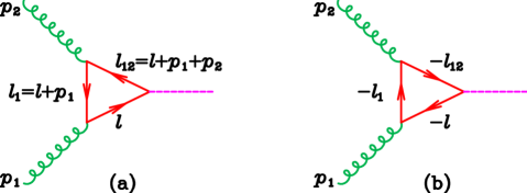
Figure 1: Triangle diagrams showing the production of a Higgs boson by gluon fusion

The first term on the right hand side of Eq. (30) already resembles the vertex for a gluon (on-shell or off-shell) interacting with a scalar field. Now consider the integrand of a triangle diagram for a Higgs boson coupled to two gluons as shown in Fig. (1a),

$$(-1)\times t^{c_{1}}t^{c_{2}}\times\frac{1}{m}\frac{{\rm tr}\{(\hbox to0.0pt{$\;\!\!\not$\hss}{\ell}+m)\gamma^{\mu_{1}}(\hbox to0.0pt{$\;\!\!\not$\hss}{\ell}_{1}+m)\gamma^{\mu_{2}}(\hbox to0.0pt{$\;\!\!\not$\hss}{\ell}_{12}+m)\}}{D(\ell)\,D(\ell_{1})\,D(\ell_{12})}\\$$

where our notation for the loop momenta and propagator factors $D(\ell)$ is given in Appendix A. The minus sign is included because of the fermion loop and an overall factor of $1/m$ has been included for convenience. By using the decomposition in Eq. (30) twice, the expression in Eq. (3.1) can be brought into the form,

$$(-1)\times t^{c_{1}}t^{c_{2}}\times\Bigg{[}\frac{{\rm tr}\{{\bf B}^{\mu_{1}}(\ell,\ell_{1}){\bf B}^{\mu_{2}}(\ell_{1},\ell_{12})\}}{D(\ell)\,D(\ell_{1})\,D(\ell_{12})}-\frac{{\rm tr}\{\gamma^{\mu_{1}}\gamma^{\mu_{2}}\}}{D(\ell)\,D(\ell_{12})}\Bigg{]}\,,$$ (31)

where ${\bf B}$ is a four-by-four matrix-valued function. It contains a convection term (as expected for a scalar field) and a spin term,

$${\bf B}^{\mu}(\ell,\ell_{1}) = (\ell^{\mu}+\ell_{1}^{\mu}){\bf 1}+\frac{1}{2}[(\hbox to0.0pt{$\;\!\!\not$\hss}{\ell}-\hbox to0.0pt{$\;\!\!\not$\hss}{\ell_{1}}),\gamma^{\mu}]\equiv(\ell^{\mu}+\ell_{1}^{\mu}){\bf 1}-\frac{1}{2}[(\hbox to0.0pt{$\;\!\!\not$\hss}{p}_{1},\gamma^{\mu}]\,.$$ (32)

Note that the spin term is independent of the loop momentum. The result for the companion triangle as shown in Fig. (1b) is

$$(-1)\times t^{c_{2}}t^{c_{1}}\times\frac{1}{m}\frac{{\rm tr}\{(-\hbox to0.0pt{$\;\!\!\not$\hss}{\ell_{12}}+m)\gamma^{\mu_{2}}(-\hbox to0.0pt{$\;\!\!\not$\hss}{\ell}_{1}+m)\gamma^{\mu_{1}}(-\hbox to0.0pt{$\;\!\!\not$\hss}{\ell}+m)\}}{D(\ell)\,D({\ell_{1}})\,D({\ell_{12})}}$$ (33)

$$= (-1)\times t^{c_{2}}t^{c_{1}}\times\Big{[}\frac{{\rm tr}\{{\bf B}^{\mu_{2}}(-\ell_{12},-\ell_{1}){\bf B}^{\mu_{1}}(-\ell_{1},-\ell)\}}{D(\ell)\,D(\ell_{1})\,D(\ell_{12})}-\frac{{\rm tr}\{\gamma^{\mu_{2}}\gamma^{\mu_{1}}\}}{D(\ell)\,D(\ell_{12})}\Big{]}\,.$$

Adding both diagrams, dropping vanishing terms and exploiting the cyclicity of the trace, the integrand appearing in the full amplitude is,

$$(-1)\Bigg{\{} t^{c_{1}}t^{c_{2}}\times\Bigg{[}\frac{(\ell^{\mu_{1}}+\ell_{1}^{\mu_{1}})(\ell_{1}^{\mu_{2}}+\ell_{12}^{\mu_{2}}){\rm tr}\{{\bf 1}\}+\frac{1}{4}{\rm tr}\{[\hbox to0.0pt{$\;\!\!\not$\hss}{p}_{1},\gamma^{\mu_{1}}][\hbox to0.0pt{$\;\!\!\not$\hss}{p}_{2},\gamma^{\mu_{2}}]\}}{D(\ell)\,D(\ell_{1})\,D(\ell_{12})}\Bigg{]}$$ (34)

$$+ t^{c_{2}}t^{c_{1}}\times\Bigg{[}\frac{(\ell^{\mu_{1}}+\ell_{1}^{\mu_{1}})(\ell_{1}^{\mu_{2}}+\ell_{12}^{\mu_{2}}){\rm tr}\{{\bf 1}\}+\frac{1}{4}{\rm tr}\{[\hbox to0.0pt{$\;\!\!\not$\hss}{p}_{1},\gamma^{\mu_{1}}][\hbox to0.0pt{$\;\!\!\not$\hss}{p}_{2},\gamma^{\mu_{2}}]\}}{D(\ell)\,D(\ell_{1})\,D(\ell_{12})}\Bigg{]}$$

$$- (t^{c_{1}}t^{c_{2}}+t^{c_{2}}t^{c_{1}})g^{\mu_{1}\mu_{2}}\frac{{{\rm tr}\{\bf 1}\}}{D(\ell)\,D(\ell_{12})}\Bigg{\}}\,.$$

If we drop the terms involving the commutators of gamma matrices, the fermionic loop (after removing an overall factor of $m$) can be written as the effect of a (suitably normalized) scalar triangle, with 3-point and 4-point (seagull) vertices. The full fermionic theory requires the inclusion of the additional spin flip terms, given by commutators. These additional terms do not involve the loop momentum and are thus of lower rank. Note also that there is no explicit mass dependence in Eq. (34). Dependence on the mass $m$ will be generated by the reduction to scalar integrals. In contrast to the full fermionic theory, we may also consider the scalar theory in the massless case.

Iterating this argument for a larger number of gluons, it can be shown that separation of the full fermionic theory into a suitably normalized scalar theory, plus spin terms involving gamma matrix commutators of rank lower by two powers of $\ell$, continues to hold. The scalar theory is obtained by dropping all of the spin terms, c.f. Eq. (32). Thus the full amplitude can be written as the sum of the scalar theory and a correction of lower rank, $\Delta F$,

$${\rm Fermion~{}theory}={\rm Scalar~{}theory}+\Delta F$$ (35)

The difference between the scalar theory and the full fermionic theory $\Delta F$ is of lower rank. Although the scalar theory contains rank-4 pentagons, rank-3 boxes, and rank-2 triangles, $\Delta F$ contains only rank-2 pentagons, rank-1 boxes and rank-0 triangles. This has several important consequences:

1. $\Delta F$ is cut constructible.

2. $\Delta F$ gives no contribution to bubble integral coefficients. Bubble integral coefficients can thus be calculated in the scalar theory.

3. $\Delta F$ gives no contribution to the $m^{2}$ contributions to triangle coefficients, $c^{(2)}_{i\times j}$.

4. $\Delta F$ gives no contribution to certain $m^{0}$ triangle coefficients, $c^{(0)}_{i\times j}$,

Exploiting these facts provides the following identities for the $ggggh$ case.

$$c_{3\times 4}(1^{+},2^{+},3^{+},4^{-}) = \tilde{c}_{3\times 4}(1^{+},2^{+},3^{+},4^{-})\,,$$

$$c_{2\times 34}(1^{+},2^{+},3^{+},4^{-}) = \tilde{c}_{2\times 34}(1^{+},2^{+},3^{+},4^{-})\,,$$

$$c_{1\times 43}(1^{+},2^{+},3^{+},4^{-}) = \tilde{c}_{1\times 43}(1^{+},2^{+},3^{+},4^{-})\,,$$ (36)

$$c_{3\times 4}(1^{+},2^{-},3^{+},4^{-}) = \tilde{c}_{3\times 4}(1^{+},2^{-},3^{+},4^{-})\,,$$

$$c_{2\times 34}(1^{+},2^{-},3^{+},4^{-}) = \tilde{c}_{2\times 34}(1^{+},2^{-},3^{+},4^{-})\,,$$ (37)

$$c_{2\times 3}(1^{+},2^{+},3^{-},4^{-}) = \tilde{c}_{2\times 3}(1^{+},2^{+},3^{-},4^{-})\,,$$

$$c_{1\times 23}(1^{+},2^{+},3^{-},4^{-}) = \tilde{c}_{1\times 23}(1^{+},2^{+},3^{-},4^{-})\,,$$ (38)

i.e. all triangles that do not have the Higgs boson as an external leg can be calculated fully in the scalar theory. In appendix C we reproduce several results for tree graphs involving massive scalars, Higgs bosons, gluons and a quark-antiquark pair. These results are useful in applying unitarity to calculate loop diagrams.

4 Coefficients for $H^{1234}_{4}(g^{+},g^{+},g^{+},g^{+};h)$

The reduction of a scalar pentagon integral into a sum of box integrals shown in Eq. (16) applies in four dimensions. Therefore an extraction of the scalar pentagon integral coefficient must be performed by making use of unitarity methods in $d$ dimensions. To this end the loop momentum is expressed most generally as,

$$\ell^{\nu}=\alpha p_{1}^{\nu}+\beta p_{2}^{\nu}+\frac{\gamma}{2}\left\langle 1|\gamma^{\nu}|2\right]+\frac{\delta}{2}\left\langle 2|\gamma^{\nu}|1\right]+\ell_{\epsilon}^{\nu}$$ (39)

where $\ell_{\epsilon}$ represents the excursion beyond four dimensions, with $\ell_{\epsilon}^{2}=-\mu^{2}$. Putting the propagators on shell determines $\alpha$, $\beta$, $\gamma$, $\delta$ and $\mu^{2}$. Parametrizing the amplitude at hand with the decomposition in Eq. (39) we thus find the pentagon coefficient,

$$e_{1\times 2\times 3\times 4}(1^{+},2^{+},3^{+},4^{+})=\frac{(m^{2}+\mu^{2})\,\left(s_{1234}-4(m^{2}+\mu^{2})\right)\,{\rm tr}_{+}\{{1}\,{2}\,{3}\,{4}\}}{\left\langle 1\,2\right\rangle\left\langle 2\,3\right\rangle\left\langle 3\,4\right\rangle\left\langle 4\,1\right\rangle}$$ (40)

where the trace functions are defined by,

$${\rm tr}_{+}\{1\,2\,3\,4\} = {\rm tr}\{\gamma_{R}\,\hbox to0.0pt{$\;\!\!\not$\hss}{p}_{1}\,\hbox to0.0pt{$\;\!\!\not$\hss}{p}_{2},\hbox to0.0pt{$\;\!\!\not$\hss}{p}_{3},\hbox to0.0pt{$\;\!\!\not$\hss}{p}_{4}\}=\left[1\,2\right]\,\left\langle 2\,3\right\rangle\,\left[3\,4\right]\left\langle 4\,1\right\rangle\,,$$

$${\rm tr}_{-}\{1\,2\,3\,4\} = {\rm tr}\{\gamma_{L}\,\hbox to0.0pt{$\;\!\!\not$\hss}{p}_{1}\,\hbox to0.0pt{$\;\!\!\not$\hss}{p}_{2},\hbox to0.0pt{$\;\!\!\not$\hss}{p}_{3},\hbox to0.0pt{$\;\!\!\not$\hss}{p}_{4}\}=\left\langle 1\,2\right\rangle\,\left[2\,3\right]\,\left\langle 3\,4\right\rangle\left[4\,1\right]\,,$$ (41)

and $\gamma_{R/L}=(1\pm\gamma_{5})/2$. The identities on the far right of Eq. (4) holds only for lightlike $p_{i}$. The value of $\mu^{2}$ is fixed by the constraint $\ell^{2}=m^{2}$ (implying $m^{2}+\mu^{2}=-\gamma\delta\,s_{12}$) but we have left the coefficient in Eq. (40) in this form in order to emphasise the $d$-dimensional nature of the result. We choose to write our amplitude in terms of an effective pentagon coefficient $\hat{e}$ that corresponds to the four-dimensional limit $\mu^{2}\to 0$,

$$\hat{e}_{1\times 2\times 3\times 4}(1^{+},2^{+},3^{+},4^{+})=\frac{m^{2}\,(s_{1234}-4m^{2}){\rm tr}_{+}\{{1}\,{2}\,{3}\,{4}\}}{\left\langle 1\,2\right\rangle\left\langle 2\,3\right\rangle\left\langle 3\,4\right\rangle\left\langle 4\,1\right\rangle}$$ (42)

This leads to a very compact form for the complete amplitude Ellis:2018hst ,

$$H_{4}^{1234}(1^{+},2^{+},3^{+},4^{+};h) = \Bigg{\{}\frac{4m^{2}-s_{1234}}{\left\langle 1\,2\right\rangle\left\langle 2\,3\right\rangle\left\langle 3\,4\right\rangle\left\langle 4\,1\right\rangle}\Big{[}-{\rm tr}_{+}\{{1}\,{2}\,{3}\,{4}\}m^{2}E_{0}(p_{1},p_{2},p_{3},p_{4};m)$$ (43)

$$+ \frac{1}{2}((s_{12}+s_{13})(s_{24}+s_{34})-s_{14}s_{23})D_{0}(p_{1},p_{23},p_{4};m)$$

$$+ \frac{1}{2}s_{12}s_{23}D_{0}(p_{1},p_{2},p_{3};m)$$

$$+ (s_{12}+s_{13}+s_{14})C_{0}(p_{1},p_{234};m)\Big{]}+2\frac{s_{12}+s_{13}+s_{14}}{\left\langle 1\,2\right\rangle\left\langle 2\,3\right\rangle\left\langle 3\,4\right\rangle\left\langle 4\,1\right\rangle}\Bigg{\}}$$

$$+ \Bigg{\{}3~{}{\rm cyclic~{}permutations}\Bigg{\}}\,.$$

Although this expression, that includes the scalar pentagon integral, is very simple, we do not follow this approach for the other helicity choices in the following sections. Instead, since in the end our aim is to produce a numerical code to calculate this amplitude, we feel that the structure is more straight-forward working only in terms of boxes, triangles and bubble coefficients. Adopting this approach also for this amplitude means that the minimal set of coefficients that must be specified corresponds to the ones shown in the first and third columns of Table 1. Note that coefficients of integrals that could in principle appear but that are not specified in this table (and in subsequent tables in later sections) vanish. There is some ambiguity in the naming convention for the integral coefficients. For a given colour-ordered amplitude the external legs will appear in cyclic or anti-cyclic order, c.f. Eq. (7). For example, $d_{1\times 2\times 34}$ in Table 1 could equally well be written as $d_{43\times 2\times 1}$. Our convention is that the vertex containing more than one gluon, should appear last in the name of the coefficient. Where the compound vertex is in the centre, we have chosen the cyclic ordering.

Coefficient	Related coefficients	Coefficient	Related coefficients
$d_{1\times 2\times 34}$	$d_{2\times 3\times 41},d_{3\times 4\times 12},d_{4\times 1\times 23},$	$c_{1\times 234}$	$c_{2\times 341},c_{3\times 412},c_{4\times 123}$
	$d_{1\times 4\times 32},d_{2\times 1\times 43},d_{3\times 2\times 14},d_{4\times 3\times 21}$
$d_{1\times 23\times 4}$	$d_{2\times 34\times 1},d_{3\times 41\times 2},d_{4\times 12\times 3}$
$d_{1\times 2\times 3}$	$d_{2\times 3\times 4},d_{3\times 4\times 1},d_{4\times 1\times 2}$

Table 1: Minimal set of integral coefficients for $1_{g}^{+}\,2_{g}^{+}\,3_{g}^{+}\,4_{g}^{+}$.

4.1 Boxes

4.1.1 $d_{1\times 2\times 34}$

$$d_{1\times 2\times 34}(1^{+},2^{+},3^{+},4^{+}) = \mathcal{C}_{1\times 2\times 3\times 4}^{(4)}\,\hat{e}_{\{1^{+}\times 2^{+}\times 3^{+}\times 4^{+}\}}$$ (44)

4.1.2 $d_{1\times 23\times 4}$

$$d_{1\times 23\times 4}(1^{+},2^{+},3^{+},4^{+}) = \mathcal{C}_{1\times 2\times 3\times 4}^{(3)}\,\hat{e}_{\{1^{+}\times 2^{+}\times 3^{+}\times 4^{+}\}}$$ (45)

$$+ \frac{1}{2}\frac{(4\,m^{2}-s_{1234})}{\left\langle 1\,2\right\rangle\left\langle 2\,3\right\rangle\left\langle 3\,4\right\rangle\left\langle 4\,1\right\rangle}\,[(s_{12}+s_{13})\,(s_{24}+s_{34})-s_{14}\,s_{23}]$$

4.1.3 $d_{1\times 2\times 3}$

$$d_{1\times 2\times 3}(1^{+},2^{+},3^{+},4^{+}) = \mathcal{C}_{4\times 1\times 2\times 3}^{(1)}\,\hat{e}_{\{4^{+}\times 1^{+}\times 2^{+}\times 3^{+}\}}+\mathcal{C}_{1\times 2\times 3\times 4}^{(5)}\,\hat{e}_{\{1^{+}\times 2^{+}\times 3^{+}\times 4^{+}\}}$$ (46)

$$+ \frac{1}{2}\frac{(4\,m^{2}-s_{1234})}{\left\langle 1\,2\right\rangle\left\langle 2\,3\right\rangle\left\langle 3\,4\right\rangle\left\langle 4\,1\right\rangle}\,s_{12}\,s_{23}$$

4.2 Triangles

4.2.1 $c_{1\times 234}^{(0)},c_{1\times 234}^{(2)}$

$$c_{1\times 234}^{(0)}(1^{+},2^{+},3^{+},4^{+}) = -(s_{12}+s_{13}+s_{14})\frac{s_{1234}}{\left\langle 1\,2\right\rangle\,\left\langle 2\,3\right\rangle\,\left\langle 3\,4\right\rangle\,\left\langle 4\,1\right\rangle}$$ (47)

$$c_{1\times 234}^{(2)}(1^{+},2^{+},3^{+},4^{+}) = 4(s_{12}+s_{13}+s_{14})\frac{1}{\left\langle 1\,2\right\rangle\,\left\langle 2\,3\right\rangle\,\left\langle 3\,4\right\rangle\,\left\langle 4\,1\right\rangle}$$ (48)

In presenting these results we have adopted the notation defined in Eq. (27) to separately quote the mass-independent and mass-dependent parts.

4.3 Rational terms

$$r(1^{+},2^{+},3^{+},4^{+}) = \frac{1}{2}\,\big{[}c_{1\times 234}^{(2)}(1^{+},2^{+},3^{+},4^{+})+c_{1\times 234}^{(2)}(2^{+},3^{+},4^{+},1^{+})$$ (49)

$$+c_{1\times 234}^{(2)}(3^{+},4^{+},1^{+},2^{+})+c_{1\times 234}^{(2)}(4^{+},1^{+},2^{+},3^{+})\big{]}$$

$$= 4\,\frac{s_{1234}}{\left\langle 1\,2\right\rangle\left\langle 2\,3\right\rangle\left\langle 3\,4\right\rangle\left\langle 4\,1\right\rangle}$$

5 Coefficients for $H^{1234}_{4}(g^{+},g^{+},g^{+},g^{-};h)$

Following the procedure outlined in Section 4 to obtain the pentagon coefficients yields, for this particular helicity combination,

$$e_{\{1^{+}\times 2^{+}\times 3^{+}\times 4^{-}\}}=-s_{12}s_{34}\left(s_{123}-4(m^{2}+\mu^{2})\right)\,\Bigg{[}\frac{\left[2\,3\right]\,\left\langle 4|(2+3)|1\right]}{{\rm tr}_{5}\{{1}\,{2}\,{3}\,{4}\}}\Bigg{]}^{2}\,,\\$$ (50)

where we have introduced the notation,

$${\rm tr}_{5}\{{1}\,{2}\,{3}\,{4}\}={\rm tr}\{\gamma_{5}\,\hbox to0.0pt{$\;\!\!\not$\hss}{p}_{1}\,\hbox to0.0pt{$\;\!\!\not$\hss}{p}_{2}\,\hbox to0.0pt{$\;\!\!\not$\hss}{p}_{3}\,\hbox to0.0pt{$\;\!\!\not$\hss}{p}_{4}\}=\left[1\,2\right]\,\left\langle 2\,3\right\rangle\,\left[3\,4\right]\,\left\langle 4\,1\right\rangle-\left\langle 1\,2\right\rangle\,\left[2\,3\right]\,\left\langle 3\,4\right\rangle\,\left[4\,1\right]\,.$$ (51)

Note that the last identity, Eq. (51), only applies for the case of lightlike momenta. At this point we could follow the same strategy as in the previous section and take the limit $\mu^{2}\to 0$ to obtain an effective pentagon coefficient $\hat{e}$. However the appearance of the factor ${\rm tr}_{5}\{{1}\,{2}\,{3}\,{4}\}$ in the denominator of Eq. (50) is unpalatable since it is an unphysical singularity. In the amplitude its presence is compensated by corresponding factors in box coefficients, and separating contributions in this way can lead to a loss of numerical precision.

As an alternative solution, we choose to modify the coefficient itself in such a way that these factors are eliminated. We do so by noting that the denominator can be expressed as,

$$\big{(}{\rm tr}_{5}\{{1}\,{2}\,{3}\,{4}\}\big{)}^{2}=(s_{12}\,s_{34}-s_{14}\,s_{23}-s_{13}\,s_{24})^{2}-4\,s_{14}\,s_{23}\,s_{24}\,s_{13}=G\,,$$ (52)

where $G$ has already been introduced in Eq. (2.2). In fact, rearranging that equation and making use of spinor notation we have,

$$s_{12}s_{23}s_{34}\left\langle 1|(2+3)|4\right]\left\langle 4|(2+3)|1\right]=m^{2}\,\big{(}{\rm tr}_{5}\{{1}\,{2}\,{3}\,{4}\}\big{)}^{2}-16\,\left|S_{1\times 2\times 3\times 4}\right|\,.$$ (53)

We may use this equation to remove the denominator $\big{(}{\rm tr}_{5}\{{1}\,{2}\,{3}\,{4}\}\big{)}^{2}$ in part of the pentagon coefficient in Eq. (50). We use Eq. (53) to eliminate one factor of $\left\langle 4|(2+3)|1\right]$ from Eq. (50). This generates two terms, one of which is free from the denominator $\big{(}{\rm tr}_{5}\{{1}\,{2}\,{3}\,{4}\}\big{)}^{2}$, which we identify as the effective pentagon coeffcient. The second term that is introduced contains a factor of $\left|S_{1\times 2\times 3\times 4}\right|$; this neatly cancels the denominator factor involved when reducing the pentagon integral to boxes (c.f. Eq. (2.2)) such that factors of $1/\big{(}{\rm tr}_{5}\{{1}\,{2}\,{3}\,{4}\}\big{)}^{2}$ can be explicitly absorbed into the box coefficients and cancelled.

In this way we arrive at effective pentagon coefficients,

$$\hat{e}_{\{1^{+}\times 2^{+}\times 3^{+}\times 4^{-}\}} = (s_{123}-4m^{2})\,m^{2}\,\Bigg{[}\frac{\left[2\,3\right]\,\left\langle 4|(2+3)|1\right]}{\left\langle 2\,3\right\rangle\,\left\langle 1|(2+3)|4\right]}\Bigg{]}\,,$$ (54)

$$\hat{e}_{\{4^{-}\times 1^{+}\times 2^{+}\times 3^{+}\}} = \hat{e}_{\{1^{+}\times 2^{+}\times 3^{+}\times 4^{-}\}}\{1\leftrightarrow 3\}\,,$$ (55)

$$\hat{e}_{\{2^{+}\times 3^{+}\times 4^{-}\times 1^{+}\}} = -m^{2}\frac{\left[2\,3\right]}{\left\langle 2\,3\right\rangle\left[3\,4\right]}\Bigg{(}\frac{\left[2\,3\right]\left\langle 2|(3+4)|1\right]\left\langle 4|(1+3)|2\right]}{\left\langle 1|(3+4)|2\right]}+\left[1\,3\right]\left\langle 4|(2+3)|1\right]$$ (56)

$$+4m^{2}\frac{\left[2\,3\right]\left\langle 3\,4\right\rangle\left\langle 2|(3+4)|1\right]}{\left\langle 2\,3\right\rangle\left\langle 1|(3+4)|2\right]}\Bigg{)}\,,$$

$$\hat{e}_{\{3^{+}\times 4^{-}\times 1^{+}\times 2^{+}\}} = \hat{e}_{\{2^{+}\times 3^{+}\times 4^{-}\times 1^{+}\}}\{1\leftrightarrow 3\}\,.$$ (57)

We will see that the box coefficients take a particularly simple form when written this way.

The minimal set of remaining integral coefficients to determine this amplitude is shown in the first and third columns of Table 2. The related coefficients included in the table are determined by using symmetry properties of the amplitude and relabelling momenta. These are mostly straightforward except for the coefficient $b_{341}$ where we have found the relation,

$$b_{341}(1^{+},2^{+},3^{+},4^{-})=-b_{234}(2^{+},3^{+},1^{+},4^{-})-b_{234}(2^{+},1^{+},3^{+},4^{-})\,.$$ (58)

Coefficient	Related coefficients	Coefficient	Related coefficients
$d_{1\times 2\times 34}$	$d_{3\times 2\times 14}$	$c_{3\times 4}$	$c_{4\times 1}$
$d_{1\times 4\times 32}$	$d_{3\times 4\times 12}$	$c_{2\times 34}$	$c_{2\times 14}$
$d_{2\times 1\times 43}$	$d_{2\times 3\times 41}$	$c_{1\times 43}$	$c_{3\times 41}$
$d_{2\times 34\times 1}$	$d_{3\times 41\times 2}$	$c_{4\times 123}$
$d_{4\times 3\times 21}$	$d_{4\times 1\times 23}$	$c_{1\times 234}$	$c_{3\times 412}$
$d_{1\times 23\times 4}$	$d_{4\times 12\times 3}$	$c_{2\times 341}$
$d_{2\times 3\times 4}$	$d_{4\times 1\times 2}$	$c_{12\times 34}$	$c_{23\times 41}$
$d_{1\times 2\times 3}$		$b_{34}$	$b_{14}$
$d_{3\times 4\times 1}$		$b_{234}$	$b_{412},b_{341}$
		$b_{1234}$

Table 2: Minimal set of integral coefficients for $1_{g}^{+}\,2_{g}^{+}\,3_{g}^{+}\,4_{g}^{-}$.

5.1 Boxes

5.1.1 $d_{1\times 2\times 34}$

$$d_{1\times 2\times 34}(1^{+},2^{+},3^{+},4^{-}) = \mathcal{C}_{1\times 2\times 3\times 4}^{(4)}\,\hat{e}_{\{1^{+}\times 2^{+}\times 3^{+}\times 4^{-}\}}$$ (59)

$$+ \frac{1}{2}\frac{\left[1\,2\right]\left[2\,3\right]\left\langle 1|(2+4)|3\right]}{\left[3\,4\right]\left\langle 1|(3+4)|2\right]\left\langle 1|(2+3)|4\right]}\Bigg{(}\left[2\,3\right]s_{1234}-4\frac{\left\langle 1|(2+4)|3\right]}{\left\langle 1\,2\right\rangle}m^{2}\Bigg{)}$$

$$- \frac{1}{2}\frac{\left[1\,2\right]\left\langle 2\,4\right\rangle\left\langle 4|(2+3)|1\right]}{\left\langle 2\,3\right\rangle\left\langle 3\,4\right\rangle\left\langle 2|(3+4)|1\right]}\Bigg{(}\left\langle 4|(2+3)|1\right]+4\frac{\left\langle 2\,4\right\rangle}{\left\langle 1\,2\right\rangle}m^{2}\Bigg{)}$$

5.1.2 $d_{1\times 4\times 32}$

$$d_{1\times 4\times 32}(1^{+},2^{+},3^{+},4^{-}) = \mathcal{C}_{2\times 3\times 4\times 1}^{(2)}\,\hat{e}_{\{2^{+}\times 3^{+}\times 4^{-}\times 1^{+}\}}$$ (60)

$$+ \frac{1}{2}\frac{\left[2\,3\right]s_{14}s_{234}}{\left\langle 2\,3\right\rangle^{2}\left[3\,4\right]\left\langle 1|(3+4)|2\right]\left\langle 1|(2+3)|4\right]}(4m^{2}s_{234}-s_{23}s_{1234})$$

5.1.3 $d_{2\times 1\times 43}$

$$d_{2\times 1\times 43}(1^{+},2^{+},3^{+},4^{-}) = \mathcal{C}_{3\times 4\times 1\times 2}^{(2)}\,\hat{e}_{\{3^{+}\times 4^{-}\times 1^{+}\times 2^{+}\}}$$ (61)

$$+ \frac{1}{2}\frac{\left[1\,2\right]\left\langle 4|(1+3)|2\right]^{2}}{\left\langle 1\,2\right\rangle\left\langle 3\,4\right\rangle\left\langle 1|(3+4)|2\right]\left\langle 3|(1+4)|2\right]}(4m^{2}\left\langle 1\,4\right\rangle-\left\langle 1\,2\right\rangle\left\langle 4|(1+3)|2\right])$$

$$+ \frac{1}{2}\frac{\left[1\,2\right]\left[1\,3\right]^{2}}{\left\langle 1\,2\right\rangle\left[1\,4\right]\left[3\,4\right]\left\langle 2|(3+4)|1\right]}(4m^{2}\left\langle 2|(1+4)|3\right]-\left\langle 2\,1\right\rangle\left[1\,3\right]s_{1234})$$

5.1.4 $d_{2\times 34\times 1}$

$$d_{2\times 34\times 1}(1^{+},2^{+},3^{+},4^{-}) = \mathcal{C}_{2\times 3\times 4\times 1}^{(3)}\,\hat{e}_{\{2^{+}\times 3^{+}\times 4^{-}\times 1^{+}\}}$$

$$+ \frac{\left\langle 2\,4\right\rangle}{\left\langle 1\,2\right\rangle\left\langle 2\,3\right\rangle}\Biggl{[}2\frac{\left\langle 1\,4\right\rangle\left\langle 2\,4\right\rangle\left\langle 1|(3+4)|2\right]\left\langle 2|(3+4)|1\right]}{\left\langle 1\,2\right\rangle^{2}\left\langle 3\,4\right\rangle}+\frac{\left\langle 4|(1+3)|2\right]\left\langle 4|(2+3)|1\right]}{2\left\langle 3\,4\right\rangle}$$

$$+ \frac{s_{1234}\left[1\,3\right]\left[2\,3\right]}{2\left[3\,4\right]}-2m^{2}\left(3\frac{\left\langle 1\,4\right\rangle\left\langle 2\,4\right\rangle\left[1\,2\right]}{\left\langle 1\,2\right\rangle\left\langle 3\,4\right\rangle}+2\frac{\left[1\,3\right]\left[2\,3\right]}{\left[3\,4\right]}+\frac{\left\langle 2\,4\right\rangle\left[1\,4\right]\left[2\,3\right]}{\left\langle 2\,3\right\rangle\left[3\,4\right]}\right)\Biggr{]}$$

5.1.5 $d_{4\times 3\times 21}$

$$d_{4\times 3\times 21}(1^{+},2^{+},3^{+},4^{-}) = \mathcal{C}_{1\times 2\times 3\times 4}^{(2)}\,\hat{e}_{\{1^{+}\times 2^{+}\times 3^{+}\times 4^{-}\}}$$ (63)

$$+ (4\,m^{2}-s_{123})\left(\frac{s_{34}\,s_{123}^{2}}{2\,\left\langle 1\,2\right\rangle\,\left\langle 2\,3\right\rangle\,\left\langle 1|(2+3)|4\right]\,\left\langle 3|(1+2)|4\right]}\right)$$

5.1.6 $d_{1\times 23\times 4}$

$$d_{1\times 23\times 4}(1^{+},2^{+},3^{+},4^{-})=\mathcal{C}_{1\times 2\times 3\times 4}^{(3)}\,\hat{e}_{\{1^{+}\times 2^{+}\times 3^{+}\times 4^{-}\}}$$ (64)

5.1.7 $d_{2\times 3\times 4}$

$$d_{2\times 3\times 4}(1^{+},2^{+},3^{+},4^{-}) = \mathcal{C}_{1\times 2\times 3\times 4}^{(1)}\,\hat{e}_{\{1^{+}\times 2^{+}\times 3^{+}\times 4^{-}\}}+\mathcal{C}_{2\times 3\times 4\times 1}^{(5)}\,\hat{e}_{\{2^{+}\times 3^{+}\times 4^{-}\times 1^{+}\}}$$ (65)

$$+ (4m^{2}s_{234}-s_{23}s_{1234})\,\frac{\left\langle 3\,4\right\rangle\left[2\,3\right]^{2}}{2\left\langle 2\,3\right\rangle\left\langle 1|(3+4)|2\right]\left\langle 1|(2+3)|4\right]}$$

5.1.8 $d_{1\times 2\times 3}$

$$d_{1\times 2\times 3}(1^{+},2^{+},3^{+},4^{-}) = \mathcal{C}_{1\times 2\times 3\times 4}^{(5)}\,\hat{e}_{\{1^{+}\times 2^{+}\times 3^{+}\times 4^{-}\}}+\mathcal{C}_{4\times 1\times 2\times 3}^{(1)}\,\hat{e}_{\{4^{-}\times 1^{+}\times 2^{+}\times 3^{+}\}}$$ (66)

$$+ (4\,m^{2}-s_{123})\,\frac{s_{123}\,\left[1\,2\right]\,\left[2\,3\right]}{2\,\left\langle 3|(1+2)|4\right]\,\left\langle 1|(2+3)|4\right]}$$

Note that, as expected, this whole expression is invariant under $1\leftrightarrow 3$ since $\mathcal{C}_{4\times 1\times 2\times 3}^{(1)}=\mathcal{C}_{3\times 2\times 1\times 4}^{(5)}$.

5.1.9 $d_{3\times 4\times 1}$

$$d_{3\times 4\times 1}(1^{+},2^{+},3^{+},4^{-}) = \mathcal{C}_{2\times 3\times 4\times 1}^{(1)}\,\hat{e}_{\{2^{+}\times 3^{+}\times 4^{-}\times 1^{+}\}}+\mathcal{C}_{3\times 4\times 1\times 2}^{(5)}\,\hat{e}_{\{3^{+}\times 4^{-}\times 1^{+}\times 2^{+}\}}$$ (67)

$$- \frac{1}{2}\frac{s_{14}\left[2\,3\right]\left\langle 3\,4\right\rangle}{\left\langle 1\,3\right\rangle\left\langle 2\,3\right\rangle^{2}\left\langle 1|(3+4)|2\right]}(\left\langle 4|(1+3)|2\right]\left\langle 2\,3\right\rangle+4m^{2}\left\langle 3\,4\right\rangle)$$

$$- \frac{1}{2}\frac{\left[1\,2\right]\left\langle 1\,4\right\rangle s_{34}}{\left\langle 1\,2\right\rangle^{2}\left\langle 1\,3\right\rangle\left\langle 3|(1+4)|2\right]}(\left\langle 4|(1+3)|2\right]\left\langle 2\,1\right\rangle+4m^{2}\left\langle 1\,4\right\rangle)$$

$$+ \frac{1}{2}\frac{\left\langle 1\,4\right\rangle\left\langle 3\,4\right\rangle}{\left\langle 1\,2\right\rangle\left\langle 1\,3\right\rangle\left\langle 2\,3\right\rangle}\Bigg{[}4\frac{s_{14}s_{34}}{\left\langle 1\,3\right\rangle}+\left[1\,3\right]\big{(}s_{123}-12m^{2}\big{)}\Bigg{]}$$

Note that this is manifestly symmetric under the exchange $1\leftrightarrow 3$.

5.2 Triangles

For the case of the triangle coefficients we divide the coefficient into two pieces, to separate the mass dependence, see Eq. (27). For many coefficients the $c_{i\times j}^{(2)}$ term is equal to zero. For these cases, the full result is given by the $m^{0}$ term and we shall omit the superscript.

5.2.1 $c_{3\times 4}$

$$c_{3\times 4}(1^{+},2^{+},3^{+},4^{-})=2s_{34}\,\frac{\left\langle 1\,4\right\rangle\left\langle 4\,3\right\rangle}{\left\langle 1\,2\right\rangle\left\langle 2\,3\right\rangle\left\langle 1\,3\right\rangle^{2}},\;\;\;$$ (68)

5.2.2 $c_{2\times 34}$

$$c_{2\times 34}(1^{+},2^{+},3^{+},4^{-}) = -2(s_{23}+s_{24})\frac{\left\langle 1\,4\right\rangle\,\left\langle 2\,4\right\rangle^{2}}{\left\langle 1\,2\right\rangle^{3}\,\left\langle 2\,3\right\rangle\,\left\langle 3\,4\right\rangle}$$ (69)

5.2.3 $c_{1\times 43}$

$$c_{1\times 43}(1^{+},2^{+},3^{+},4^{-})=-2(s_{13}+s_{14})\;\frac{(\left\langle 1\,2\right\rangle\left\langle 3\,4\right\rangle+\left\langle 1\,3\right\rangle\left\langle 2\,4\right\rangle)}{\left\langle 1\,2\right\rangle\left\langle 3\,4\right\rangle}\Big{[}\frac{\left\langle 1\,4\right\rangle}{\left\langle 1\,2\right\rangle\left\langle 1\,3\right\rangle}\Big{]}^{2},\;\;\;$$ (70)

5.2.4 $c_{4\times 123}^{(0)},c_{4\times 123}^{(2)}$

$$c^{(0)}_{4\times 123}(1^{+},2^{+},3^{+},4^{-}) = -\frac{s_{123}^{2}\,(s_{14}+s_{24}+s_{34})}{\left\langle 1\,2\right\rangle\,\left\langle 2\,3\right\rangle\,\left\langle 3|(1+2)|4\right]\,\left\langle 1|(2+3)|4\right]}$$ (71)

$$c^{(2)}_{4\times 123}(1^{+},2^{+},3^{+},4^{-}) = 4\frac{s_{123}\,(s_{14}+s_{24}+s_{34})}{\left\langle 1\,2\right\rangle\,\left\langle 2\,3\right\rangle\,\left\langle 3|(1+2)|4\right]\,\left\langle 1|(2+3)|4\right]}$$ (72)

5.2.5 $c_{1\times 234}^{(0)},c_{1\times 234}^{(2)}$

$$c^{(0)}_{1\times 234}(1^{+},2^{+},3^{+},4^{-})=-2\frac{\left\langle 1|(2+3)|1\right]^{2}\left\langle 4|(2+3)|1\right]}{\left\langle 1|(2+3)|4\right]\left\langle 1\,2\right\rangle\left\langle 2\,3\right\rangle\left\langle 3\,4\right\rangle\left[1\,4\right]}$$

$$+(s_{12}+s_{13}+s_{14})\Bigg{[}\frac{1}{\left\langle 1|(2+3)|4\right]}\left(2\frac{\left\langle 4|(2+3)|1\right]\left[2\,3\right]^{2}}{s_{34}s_{234}}-\frac{(s_{12}+s_{13})^{2}\left[3\,4\right]+s_{23}\left\langle 1\,2\right\rangle\left[2\,3\right]\left[1\,4\right]}{\left\langle 1\,2\right\rangle\left\langle 1\,3\right\rangle\left\langle 2\,3\right\rangle\left[1\,4\right]\left[3\,4\right]}\right)$$

$$+\frac{\left\langle 3|(1+4)|2\right]\left\langle 1\,4\right\rangle\left[2\,3\right]^{2}}{\left\langle 1|(3+4)|2\right]\left\langle 1\,2\right\rangle\left\langle 1\,3\right\rangle\left[2\,4\right]s_{34}}-\frac{\left\langle 4|(2+3)|1\right]\left[1\,3\right]^{2}}{\left\langle 2|(3+4)|1\right]\left\langle 1\,2\right\rangle\left[1\,4\right]s_{34}}-\frac{\left\langle 1\,4\right\rangle(s_{12}^{2}\left\langle 2\,3\right\rangle+2\left\langle 1\,3\right\rangle\left\langle 2\,4\right\rangle\left[1\,4\right]s_{24})}{\left\langle 1\,2\right\rangle^{3}\left\langle 2\,3\right\rangle\left\langle 1\,3\right\rangle\left\langle 3\,4\right\rangle\left[2\,4\right]\left[1\,4\right]}\Bigg{]}$$

$$c_{1\times 234}^{(2)}(1^{+},2^{+},3^{+},4^{-}) = \frac{8\,\left\langle 4|(2+3)|1\right]^{3}}{s_{234}\,(s_{12}+s_{13}+s_{14})\,\left\langle 2\,3\right\rangle\,\left\langle 3\,4\right\rangle\,\left\langle 2|(3+4)|1\right]}$$ (74)

$$- 4\,(s_{12}+s_{13}+s_{14})\Bigg{\{}\frac{\left\langle 1\,4\right\rangle^{2}\,\left[2\,3\right]}{\left\langle 1\,2\right\rangle^{2}\,\left\langle 3\,4\right\rangle\,\left\langle 1|(3+4)|2\right]\,\left\langle 1|(2+3)|4\right]}$$

$$- \frac{\left[2\,3\right]}{\left\langle 1\,2\right\rangle\,\left\langle 1|(2+3)|4\right]\,\left\langle 1|(3+4)|2\right]\,\left\langle 2|(3+4)|1\right]}\Big{[}\frac{\left\langle 1\,2\right\rangle\left[1\,3\right]\left[2\,3\right]}{\left[3\,4\right]}+\frac{\left[1\,2\right]\left\langle 1\,4\right\rangle\left\langle 2\,4\right\rangle}{\left\langle 3\,4\right\rangle}\Big{]}$$

$$- \Big{[}\frac{\left[1\,3\right]\,\left\langle 1\,4\right\rangle}{\left\langle 1\,2\right\rangle}+\frac{\left\langle 4|(2+3)|1\right]}{\left\langle 2\,3\right\rangle}\Big{]}\Big{[}\frac{\left\langle 2\,4\right\rangle}{\left\langle 1\,2\right\rangle\,\left\langle 3\,4\right\rangle\,\left\langle 1|(2+3)|4\right]\,\left\langle 2|(3+4)|1\right]}\Big{]}\Bigg{\}}$$

5.2.6 $c_{2\times 341}^{(0)},c_{2\times 341}^{(2)}$

$$c_{2\times 341}^{(0)}(1^{+},2^{+},3^{+},4^{-})=2\frac{(s_{12}+s_{23}+s_{24})\left\langle 2\,4\right\rangle^{2}\big{(}\left\langle 1\,4\right\rangle^{2}\left\langle 2\,3\right\rangle^{2}+\left\langle 1\,2\right\rangle^{2}\left\langle 3\,4\right\rangle^{2}\big{)}}{\left\langle 1\,2\right\rangle^{3}\left\langle 2\,3\right\rangle^{3}\left\langle 1\,4\right\rangle\left\langle 3\,4\right\rangle}$$ (75)

$$+ \frac{\left\langle 4|(1+3)|2\right]^{4}}{s_{134}\left\langle 1\,4\right\rangle\left\langle 3\,4\right\rangle\left\langle 1|(3+4)|2\right]\left\langle 3|(1+4)|2\right]}+\frac{(s_{12}+s_{23})\left[1\,3\right]^{2}}{\left\langle 1\,2\right\rangle\left[1\,4\right]\left\langle 2\,3\right\rangle\left[3\,4\right]}$$

$$+ \left\{\frac{(s_{12}+s_{23}+s_{24})\left[1\,2\right]\left[1\,3\right]^{3}}{s_{134}\left[1\,4\right]\left[3\,4\right]\left\langle 2|(3+4)|1\right]}-\frac{\left[1\,2\right]\left\langle 2\,4\right\rangle^{2}\left\langle 4|(3+2)|1\right]}{\left\langle 1\,2\right\rangle\left\langle 2\,3\right\rangle\left\langle 3\,4\right\rangle\left\langle 2|(3+4)|1\right]}-\frac{\left[1\,2\right]\left[1\,3\right]^{2}\left\langle 2\,4\right\rangle}{\left\langle 2\,3\right\rangle\left[3\,4\right]\left\langle 2|(3+4)|1\right]}\right\}$$

$$+ \{1\leftrightarrow 3\}$$

$$c_{2\times 341}^{(2)}(1^{+},2^{+},3^{+},4^{-}) = \frac{4(s_{12}+s_{23}+s_{24})\,s_{134}\,\left[1\,2\right]\,\left[3\,2\right]}{\left\langle 1\,2\right\rangle\,\left\langle 3\,2\right\rangle\,\left[1\,4\right]\,\left[3\,4\right]\,\left\langle 1|(3+4)|2\right]\,\left\langle 3|(1+4)|2\right]}$$ (76)

$$- \frac{8}{(s_{12}+s_{23}+s_{24})\,s_{134}}\frac{\left\langle 4|(1+3)|2\right]^{4}}{\left\langle 1\,4\right\rangle\,\left\langle 3\,4\right\rangle\,\left\langle 1|(3+4)|2\right]\,\left\langle 3|(1+4)|2\right]}$$

$$+ \Bigg{\{}\frac{4\,(s_{12}+s_{23}+s_{24})}{[(s_{13}+s_{14})\,(s_{23}+s_{24})-s_{12}\,s_{34}]}\Big{[}\frac{\left[1\,3\right]^{2}\,\left[2\,3\right]}{\left\langle 1\,2\right\rangle\,\left[1\,4\right]\,\left[3\,4\right]}-\frac{\left[1\,2\right]\,\left\langle 1\,4\right\rangle\,\left\langle 2\,4\right\rangle^{2}}{\left\langle 1\,2\right\rangle^{2}\,\left\langle 2\,3\right\rangle\,\left\langle 3\,4\right\rangle}\Big{]}\Bigg{\}}$$

$$+ \Big{\{}1\leftrightarrow 3\Big{\}}$$

5.2.7 $c_{12\times 34}^{(0)},c_{12\times 34}^{(2)}$

$$c^{(0)}_{12\times 34}(1^{+},2^{+},3^{+},4^{-}) = \frac{\left[1\,3\right]\,(s_{12}+s_{23})\,\left\langle 4|(2+3)|1\right]}{\left\langle 1\,2\right\rangle\,\left\langle 2\,3\right\rangle\,\left[2\,4\right]\,\left\langle 2|(3+4)|1\right]}+\frac{\left[1\,2\right]\,\left\langle 2\,4\right\rangle^{2}\,\left\langle 4|(2+3)|1\right]}{\left\langle 1\,2\right\rangle\,\left\langle 2\,3\right\rangle\,\left\langle 3\,4\right\rangle\,\left\langle 2|(3+4)|1\right]}$$ (77)

$$- \frac{\left[2\,3\right]\,\left\langle 4|(1+3)|2\right]^{2}}{\left\langle 1\,2\right\rangle\,\left[2\,4\right]\,\left\langle 3\,4\right\rangle\,\left\langle 1|(3+4)|2\right]}-\frac{\left[2\,3\right]^{3}\,s_{1234}}{\left\langle 1\,2\right\rangle\,\left[2\,4\right]\,\left[3\,4\right]\,\left\langle 1|(3+4)|2\right]}$$

$$- \frac{\left[1\,3\right]^{2}\,\left[2\,3\right]\,s_{1234}}{\left\langle 1\,2\right\rangle\,\left[2\,4\right]\,\left[3\,4\right]\,\left\langle 2|(3+4)|1\right]}+\frac{\left[1\,2\right]\,s_{123}\,(s_{123}-s_{124})}{\left\langle 1\,2\right\rangle\,\left\langle 2\,3\right\rangle\,\left[2\,4\right]\,\left\langle 3|(1+2)|4\right]}$$

$$- \frac{\left[1\,2\right]\,\left\langle 1\,4\right\rangle\,\left\langle 4|(2+3)|1\right]}{\left\langle 1\,2\right\rangle\,\left\langle 2\,3\right\rangle\,\left[2\,4\right]\,\left\langle 3\,4\right\rangle}$$

$$c_{12\times 34}^{(2)}(1^{+},2^{+},3^{+},4^{-}) = -4\,\frac{\left[1\,2\right]}{\left\langle 1\,2\right\rangle\,\left\langle 3|(1+2)|4\right]\,\big{[}(s_{13}+s_{14})\,(s_{23}+s_{24})-s_{12}\,s_{34}\big{]}}$$ (78)

$$\times \Bigg{[}\left(\left\langle 1\,4\right\rangle\,\left[1\,3\right]-\left\langle 2\,4\right\rangle\,\left[2\,3\right]\right)(s_{13}+s_{23}-s_{14}-s_{24})$$

$$+ \left\langle 1\,2\right\rangle\,\left\langle 3\,4\right\rangle\,\left[1\,3\right]\,\left[2\,3\right]\,\left(2-\frac{(s_{13}+s_{23})\,(s_{13}+s_{14}+s_{23}+s_{24})}{s_{12}\,s_{34}}\right)$$

$$+ \left\langle 1\,4\right\rangle\,\left\langle 2\,4\right\rangle\,\left[1\,2\right]\,\left[3\,4\right]\,\left(2-\frac{(s_{14}+s_{24})\,(s_{13}+s_{14}+s_{23}+s_{24})}{s_{12}\,s_{34}}\right)\Bigg{]}$$

5.3 Bubbles

5.3.1 $b_{34}$

$$b_{34}(1^{+},2^{+},3^{+},4^{-})=\frac{4}{\left\langle 1\,2\right\rangle^{2}\left\langle 1\,3\right\rangle\left\langle 2\,3\right\rangle}\left(\frac{\left\langle 2\,4\right\rangle^{2}\left\langle 1\,3\right\rangle\left[2\,3\right]}{(s_{23}+s_{24})}-\frac{\left\langle 1\,4\right\rangle^{2}\left\langle 2\,3\right\rangle\left[1\,3\right]}{(s_{13}+s_{14})}\right)$$ (79)

5.3.2 $b_{234}$

$$b_{234}(1^{+},2^{+},3^{+},4^{-}) = \frac{4}{\left\langle 2\,3\right\rangle\,\left\langle 3\,4\right\rangle}\Bigg{(}\frac{\left\langle 2\,4\right\rangle^{2}\,\left\langle 4|(2+3)|1\right]}{\left\langle 1\,2\right\rangle^{2}\,\left\langle 2|(3+4)|1\right]}$$ (80)

$$- \frac{\left\langle 4|(2+3)|1\right]^{3}}{\left\langle 2|(3+4)|1\right]\,(s_{1234}-s_{234})^{2}}-\frac{\left\langle 2\,4\right\rangle^{2}\,\left[2\,3\right]\,\left\langle 3\,4\right\rangle}{\left\langle 1\,2\right\rangle^{2}\,(s_{23}+s_{24})}\Bigg{)}$$

5.3.3 $b_{1234}$

Since the full amplitude is finite in four dimensions, one of the coefficients is uniquely determined in terms of the remainder. We thus have,

$$b_{1234}(1^{+},2^{+},3^{+},4^{-})=-b_{34}-b_{41}-b_{234}-b_{412}-b_{341}\,,$$ (81)

where we have suppressed momentum and helicity labels on the right-hand side for brevity.

5.4 Rational terms

$$r(1^{+},2^{+},3^{+},4^{-}) = \frac{1}{2}\big{[}c_{12\times 34}^{(2)}(1^{+},2^{+},3^{+},4^{-})+c_{12\times 34}^{(2)}(3^{+},2^{+},1^{+},4^{-})$$ (82)

$$+ c_{1\times 234}^{(2)}(1^{+},2^{+},3^{+},4^{-})+c_{1\times 234}^{(2)}(3^{+},2^{+},1^{+},4^{-})$$

$$+ c_{4\times 123}^{(2)}(1^{+},2^{+},3^{+},4^{-})+c_{2\times 341}^{(2)}(1^{+},2^{+},3^{+},4^{-})\big{]}$$

6 Coefficients for $H^{1234}_{4}(g^{+},g^{-},g^{+},g^{-};h)$

For this helicity combination the coefficients of the scalar pentagon integrals contain a factor of $1/{\rm tr}_{5}\{{1}\,{2}\,{3}\,{4}\}^{4}$ and we must modify the pentagon integral coefficients in a similar fashion as described for the $+++-$ configuration in Section 5. All coefficients can then be written in terms of a single function,

$$\hat{e}_{\{1^{+}\times 2^{-}\times 3^{+}\times 4^{-}\}}=-m^{2}\frac{\left\langle 1\,2\right\rangle\left[3\,4\right]\left\langle 4|(2+3)|1\right]}{\left[1\,2\right]\left\langle 3\,4\right\rangle\left\langle 1|(2+3)|4\right]}\Bigg{(}\frac{\left[1\,3\right]^{2}\left\langle 3\,4\right\rangle}{\left[3\,4\right]}+\frac{\left\langle 2\,4\right\rangle^{2}\left[1\,2\right]}{\left\langle 1\,2\right\rangle}+4m^{2}\frac{\left\langle 4|(2+3)|1\right]}{\left\langle 1|(2+3)|4\right]}\Bigg{)}$$ (83)

This is manifestly symmetric under $\bigl{\{}1\leftrightarrow 4,\,2\leftrightarrow 3,\langle\rangle\leftrightarrow[]\bigr{\}}$. Other coefficients are trivially related via symmetries:

$$\hat{e}_{\{3^{+}\times 4^{-}\times 1^{+}\times 2^{-}\}} = \hat{e}_{\{1^{+}\times 2^{-}\times 3^{+}\times 4^{-}\}}\Bigl{\{}1\leftrightarrow 3,\,2\leftrightarrow 4\Bigr{\}}$$ (84)

$$\hat{e}_{\{4^{-}\times 1^{+}\times 2^{-}\times 3^{+}\}} = \hat{e}_{\{1^{+}\times 2^{-}\times 3^{+}\times 4^{-}\}}\Bigl{\{}1\to 4,\,2\to 1,\,3\to 2,\,4\to 3,\,\langle\rangle\leftrightarrow[]\Bigr{\}}$$ (85)

$$\hat{e}_{\{2^{-}\times 3^{+}\times 4^{-}\times 1^{+}\}} = \hat{e}_{\{1^{+}\times 2^{-}\times 3^{+}\times 4^{-}\}}\Bigl{\{}1\to 2,\,2\to 3,\,3\to 4,\,4\to 1,\,\langle\rangle\leftrightarrow[]\Bigr{\}}$$ (86)

The minimal set of integral coefficients that must be calculated for the colour ordering $H_{4}^{1234}$ is shown in the first and third columns of Table 3, for example the bubble coefficients are given by:

$$b_{412}(1^{+},2^{-},3^{+},4^{-}) = b_{234}(3^{+},4^{-},1^{+},2^{-})$$

$$b_{123}(1^{+},2^{-},3^{+},4^{-}) = b_{234}(4^{+},1^{-},2^{+},3^{-})|_{\langle\,\rangle\leftrightarrow[\,]}$$

$$b_{341}(1^{+},2^{-},3^{+},4^{-}) = b_{234}(2^{+},3^{-},4^{+},1^{-})|_{\langle\,\rangle\leftrightarrow[\,]}\,.$$ (87)

The calculation of the coefficients of other colour orderings requires the use of $+\,+\,-\,-$ functions which are given in the next section.

Coefficient	Related coefficients	Coefficient	Related coefficients
$d_{4\times 3\times 21}$	$d_{2\times 1\times 43},d_{3\times 2\times 14},d_{1\times 4\times 32},$	$c_{3\times 4}$	$c_{4\times 1},c_{2\times 3},c_{1\times 2}$
	$d_{1\times 2\times 34},d_{2\times 3\times 41},$	$c_{2\times 34}$	$c_{3\times 41},c_{4\times 12},c_{1\times 23}$
	$d_{3\times 4\times 12},d_{4\times 1\times 23}$		$c_{1\times 43},c_{2\times 14},c_{3\times 21},c_{4\times 32}$
$d_{1\times 23\times 4}$	$d_{2\times 34\times 1},d_{3\times 41\times 2},d_{4\times 12\times 3}$	$c_{12\times 34}$	$c_{23\times 41}$
$d_{1\times 2\times 3}$	$d_{2\times 3\times 4},d_{3\times 4\times 1},d_{4\times 1\times 2}$	$c_{1\times 234}$	$c_{2\times 341},c_{3\times 412},c_{4\times 123}$
		$b_{34}$	$b_{12},b_{23},b_{41}$
		$b_{234}$	$b_{341},b_{412},b_{123}$
		$b_{1234}$

Table 3: Minimal set of integral coefficients for $1_{g}^{+}\,2_{g}^{-}\,3_{g}^{+}\,4_{g}^{-}$.

6.1 Boxes

6.1.1 $d_{4\times 3\times 21}$

$$d_{4\times 3\times 21}(1^{+},2^{-},3^{+},4^{-}) = \hat{e}_{\{1^{+}\times 2^{-}\times 3^{+}\times 4^{-}\}}\,\mathcal{C}_{1\times 2\times 3\times 4}^{(2)}$$ (88)

$$+ \frac{\left\langle 2|(1+3)|4\right]}{\left\langle 1|(2+3)|4\right]\left\langle 3|(1+2)|4\right]}\Bigg{[}-2\frac{\left\langle 2\,3\right\rangle\left\langle 2|(1+3)|4\right]s_{34}s_{123}^{2}}{\left\langle 1\,2\right\rangle\left\langle 3|(1+2)|4\right]^{2}}$$

$$+ \frac{1}{2}\frac{\left\langle 2\,4\right\rangle^{2}\left[3\,4\right]s_{123}}{\left\langle 1\,2\right\rangle}+\frac{1}{2}\frac{\left[1\,3\right]^{2}\left\langle 3\,4\right\rangle s_{123}}{\left[1\,2\right]}-2m^{2}\Bigg{(}2\frac{\left[1\,3\right]\left\langle 4|(2+3)|1\right]}{\left[1\,2\right]}$$

$$+ \frac{\left[2\,3\right]\left\langle 2|(1+3)|4\right]\left\langle 4|(2+3)|1\right]}{\left[1\,2\right]\left\langle 1|(2+3)|4\right]}+3\frac{\left\langle 2\,3\right\rangle\left\langle 2|(1+3)|4\right]\left\langle 4|(1+2)|3\right]}{\left\langle 1\,2\right\rangle\left\langle 3|(1+2)|4\right]}\Bigg{)}\Bigg{]}$$

6.1.2 $d_{1\times 23\times 4}$

$$d_{1\times 23\times 4}(1^{+},2^{-},3^{+},4^{-}) = \hat{e}_{\{1^{+}\times 2^{-}\times 3^{+}\times 4^{-}\}}\,\mathcal{C}_{1\times 2\times 3\times 4}^{(3)}$$ (89)

$$+ \Bigg{[}\frac{1}{2}\frac{\left\langle 2\,4\right\rangle^{3}\left\langle 4|(2+3)|1\right]}{\left\langle 2\,3\right\rangle\left\langle 3\,4\right\rangle\left\langle 4\,1\right\rangle}\Bigg{(}1+4m^{2}\frac{\left\langle 1\,2\right\rangle}{\left\langle 2\,4\right\rangle\left\langle 1|(2+3)|4\right]}\Bigg{)}\Bigg{]}$$

$$+ \Big{[}1\leftrightarrow 4,\,2\leftrightarrow 3,\langle\rangle\leftrightarrow[]\Big{]}$$

Note that here the symmetrization only applies to the terms in square brackets.

6.1.3 $d_{1\times 2\times 3}$

$$d_{1\times 2\times 3}(1^{+},2^{-},3^{+},4^{-}) = \mathcal{C}_{1\times 2\times 3\times 4}^{(5)}\,\hat{e}_{\{1^{+}\times 2^{-}\times 3^{+}\times 4^{-}\}}+\mathcal{C}_{4\times 1\times 2\times 3}^{(1)}\,\hat{e}_{\{4^{-}\times 1^{+}\times 2^{-}\times 3^{+}\}}$$ (90)

$$+ \frac{\left\langle 1\,2\right\rangle\left\langle 2\,3\right\rangle}{\left\langle 1|(2+3)|4\right]\left\langle 3|(1+2)|4\right]}\Bigg{[}-2\frac{s_{12}s_{23}s_{123}}{\left\langle 1\,3\right\rangle^{2}}-\frac{1}{2}\frac{\left[1\,2\right]\left[2\,3\right]\left\langle 2\,4\right\rangle^{2}(s_{14}+s_{24}+s_{34})}{\left\langle 1\,4\right\rangle\left\langle 3\,4\right\rangle}$$

$$+ \frac{1}{2}\left[1\,3\right]^{2}s_{123}+2m^{2}\Bigg{(}2\frac{\left[1\,3\right]s_{123}}{\left\langle 1\,3\right\rangle}-\left[1\,3\right]^{2}+\frac{\left[1\,2\right]\left[2\,3\right]\left\langle 2\,4\right\rangle^{2}}{\left\langle 1\,4\right\rangle\left\langle 3\,4\right\rangle}$$

$$- \frac{\left[2\,3\right]\left\langle 2|(1+3)|4\right]\left\langle 4|(2+3)|1\right]}{\left\langle 3\,4\right\rangle\left\langle 1|(2+3)|4\right]}+\frac{\left[1\,2\right]\left\langle 2|(1+3)|4\right]\left\langle 4|(1+2)|3\right]}{\left\langle 1\,4\right\rangle\left\langle 3|(1+2)|4\right]}\Bigg{)}\Bigg{]}$$

Note that this is explicitly symmetric under the exchange $1\leftrightarrow 3$.

6.2 Triangles

6.2.1 $c_{3\times 4}$

$$c_{3\times 4}(1^{+},2^{-},3^{+},4^{-})=\frac{-2s_{34}}{s_{12}\left\langle 3|(1+2)|4\right]^{3}\left\langle 1\,3\right\rangle^{2}\left[2\,4\right]^{2}}$$

$$\left\{\left\langle 3|1|4\right]^{3}\left[s_{24}(s_{14}+s_{24})+s_{12}(s_{23}+s_{34})\right]+\left\langle 3|1|4\right]^{2}\left\langle 3|2|4\right]\left[s_{12}^{2}-s_{14}(s_{14}+s_{24})+s_{12}(3s_{234}-5s_{24})\right]\right.$$

$$\left.+\left\langle 3|2|4\right]^{3}\left[s_{13}(s_{13}+s_{23})+s_{12}(s_{14}+s_{34})\right]+\left\langle 3|1|4\right]\left\langle 3|2|4\right]^{2}\left[s_{12}^{2}-s_{23}(s_{13}+s_{23})+s_{12}(3s_{134}-5s_{13})\right]\right\}$$

6.2.2 $c_{2\times 34}$

$$c_{2\times 34}(1^{+},2^{-},3^{+},4^{-}) = 2(s_{23}+s_{24})\frac{s_{234}\,\left[2\,3\right]^{2}\Big{(}\left\langle 1|(2+4)|3\right]\,\left[2\,4\right]+\left\langle 1|(3+4)|2\right]\,\left[3\,4\right]\Big{)}}{\left\langle 1|(3+4)|2\right]^{3}\,\left[2\,4\right]^{2}\,\left[3\,4\right]}$$ (92)

6.2.3 $c_{12\times 34}^{(0)},c_{12\times 34}^{(2)}$

This coefficient is defined in terms of the corresponding coefficient with a scalar loop, $\tilde{c}^{(0)}_{12\times 34}$

$$c^{(0)}_{12\times 34}(1^{+},2^{-},3^{+},4^{-}) = \tilde{c}^{(0)}_{12\times 34}(1^{+},2^{-},3^{+},4^{-})$$

$$+ \Bigg{\{}\frac{\left\langle 2\,1\right\rangle^{2}\,\left[1\,3\right]^{2}\,\left\langle 3\,4\right\rangle^{2}-\left\langle 2\,4\right\rangle^{2}\,\left\langle 1|(3+4)|1\right]\,\left\langle 4|(1+2)|4\right]}{\left\langle 1\,2\right\rangle\,\left\langle 3\,4\right\rangle\,\left\langle 1|(3+4)|2\right]\,\left\langle 3|(1+2)|4\right]}\Bigg{\}}$$

$$+ \Big{\{}1\leftrightarrow 3,2\leftrightarrow 4\Big{\}}+\Big{\{}1\leftrightarrow 2,3\leftrightarrow 4,\langle\,\rangle\leftrightarrow[\,]\Big{\}}+\Big{\{}1\leftrightarrow 4,2\leftrightarrow 3,\langle\,\rangle\leftrightarrow[\,]\Big{\}}$$

$$c_{12\times 34}^{(2)}(1^{+},2^{-},3^{+},4^{-}) = \Bigg{\{}4\frac{\left\langle 2|(3+4)|1\right]}{\left\langle 1|(3+4)|2\right]\left\langle 3|(1+2)|4\right]}\Biggl{[}\frac{\left[2\,3\right]^{2}\left(s_{23}-s_{14}\right)}{\left[1\,2\right]\left[3\,4\right]\left\langle 1|(3+4)|2\right]}+\frac{3}{2}\frac{\left[1\,3\right]\left[2\,3\right]}{\left[1\,2\right]\left[3\,4\right]}$$

$$+ \left\langle 2\,4\right\rangle\frac{\left(\left\langle 3|(1+2)|3\right]-\left\langle 4|(1+2)|4\right]\right)}{\Delta_{3}(1,2,3,4)}\left(\left[2\,3\right]-\frac{\left\langle 1\,4\right\rangle p_{12}\cdot p_{34}}{\left\langle 1\,2\right\rangle\left\langle 3\,4\right\rangle}\right)\Bigg{]}\Bigg{\}}$$

$$+ \Big{\{}1\leftrightarrow 3,2\leftrightarrow 4\Big{\}}+\Big{\{}1\leftrightarrow 2,3\leftrightarrow 4,\langle\,\rangle\leftrightarrow[\,]\Big{\}}+\Big{\{}1\leftrightarrow 4,2\leftrightarrow 3,\langle\,\rangle\leftrightarrow[\,]\Big{\}}$$

where $\Delta_{3}$ is given by Eq. (174).

The coefficient for a scalar loop is,

$$\tilde{c}_{12\times 34}^{(0)}(1^{+},2^{-},3^{+},4^{-})=\Bigg{\{}2\,\frac{\left\langle 2\,3\right\rangle^{3}\,\left[3\,4\right]\,\left\langle 3|(1+2)|3\right]\,(\left\langle 3|(1+2)|3\right]\,\left[2\,3\right]-\left[1\,2\right]\,\left\langle 1\,4\right\rangle\,\left[3\,4\right])}{\left\langle 1\,2\right\rangle\,\left\langle 1|(3+4)|2\right]\,\left\langle 3|(1+2)|4\right]^{3}}$$ (95)

$$+ 2\,\frac{\left\langle 2\,3\right\rangle^{2}\,\left[3\,4\right]\,\left\langle 4|(1+2)|3\right]\,(-2\,s_{23}-s_{24})}{\left\langle 1\,2\right\rangle\,\left\langle 1|(3+4)|2\right]\,\left\langle 3|(1+2)|4\right]^{2}}$$

$$+ 2\,\frac{\left[1\,2\right]\left\langle 2\,3\right\rangle^{2}\left[3\,4\right](2s_{12}(s_{23}-s_{14}-s_{34})+2s_{13}s_{23}+2s_{23}^{2}+s_{14}s_{34}-s_{23}s_{34}+2\left[1\,2\right]\left\langle 1\,3\right\rangle\left\langle 2\,4\right\rangle\left[3\,4\right])}{\left\langle 1|(3+4)|2\right]\left\langle 3|(1+2)|4\right]^{3}}$$

$$+ 2\,\frac{\left[1\,4\right]^{2}(\left\langle 1\,4\right\rangle\left\langle 2\,4\right\rangle(2(s_{13}-s_{24})-3(s_{34}+s_{14})-4(s_{12}+s_{23}))-2\left\langle 1\,3\right\rangle\left[2\,3\right]\left\langle 2\,4\right\rangle^{2}+3\left[1\,3\right]\left\langle 1\,4\right\rangle^{2}\left\langle 2\,3\right\rangle)}{\left\langle 1|(3+4)|2\right]\left\langle 3|(1+2)|4\right]^{2}}$$

$$+ \frac{s_{14}^{2}\,s_{12}\,(6\,s_{13}-2\,s_{14}+2\,s_{23}+2\,s_{24})-s_{14}^{4}+s_{14}^{2}\,s_{23}^{2}}{\left\langle 1|(3+4)|2\right]^{2}\,\left\langle 3|(1+2)|4\right]^{2}}-8\,\frac{s_{12}\,s_{13}\,s_{14}\,s_{23}}{\left\langle 1|(3+4)|2\right]^{2}\,\left\langle 3|(1+2)|4\right]^{2}}$$

$$+ 4\,\frac{s_{14}\,s_{1234}\,\left\langle 2|(3+4)|1\right]\,\left\langle 4|(1+2)|3\right]}{\left\langle 1|(3+4)|2\right]\,\left\langle 3|(1+2)|4\right]\,\Delta_{3}(1,2,3,4)}+4\,\frac{\left\langle 1\,2\right\rangle\,\left[1\,3\right]\,\left\langle 2|(3+4)|1\right]\,\left\langle 4|(1+2)|3\right]\,\left\langle 3|(1+4)|2\right]}{\left\langle 1|(3+4)|2\right]\,\left\langle 3|(1+2)|4\right]\,\Delta_{3}(1,2,3,4)}$$

$$+ \frac{\left\langle 1|(2+3)|4\right]\,\left\langle 2|(3+4)|1\right]\,\left\langle 3|(1+4)|2\right]\,\left\langle 4|(1+2)|3\right]\,(\Pi(4,3,2,1)\,\Pi(1,2,3,4)+\Delta_{3}(1,2,3,4))}{\left\langle 1|(3+4)|2\right]^{2}\,\left\langle 3|(1+2)|4\right]^{2}\,\Delta_{3}(1,2,3,4)}$$

$$- 3\,\frac{s_{1234}\,\left\langle 2|(3+4)|1\right]\,\left\langle 4|(1+2)|3\right]\,\Pi(4,3,2,1)\,\Pi(1,2,3,4)\,(s_{13}+s_{14}+s_{23}+s_{24})}{2\,\left\langle 1|(3+4)|2\right]\,\left\langle 3|(1+2)|4\right]\,\Delta_{3}(1,2,3,4)^{2}}$$

$$+ 5\,\frac{s_{1234}\,\left\langle 2|(3+4)|1\right]\,\left\langle 4|(1+2)|3\right]\,(s_{13}+s_{14}+s_{23}+s_{24})}{2\,\left\langle 1|(3+4)|2\right]\,\left\langle 3|(1+2)|4\right]\,\Delta_{3}(1,2,3,4)}-4\,\frac{\left\langle 2|(3+4)|1\right]\,\left\langle 4|(1+2)|3\right]}{\left\langle 1|(3+4)|2\right]\,\left\langle 3|(1+2)|4\right]}\Bigg{\}}$$

$$+ \Big{\{}1\leftrightarrow 3,2\leftrightarrow 4\Big{\}}+\Big{\{}1\leftrightarrow 2,3\leftrightarrow 4,\langle\,\rangle\leftrightarrow[\,]\Big{\}}+\Big{\{}1\leftrightarrow 4,2\leftrightarrow 3,\langle\,\rangle\leftrightarrow[\,]\Big{\}}$$

where

$$\Pi(i,j,k,l)=s_{ik}+s_{jk}-s_{il}-s_{jl}$$ (96)

and $\Delta_{3}$ is given by Eq. (174).

6.2.4 $c_{1\times 234}^{(0)},c_{1\times 234}^{(2)}$

$$c_{1\times 234}^{(0)}(1^{+},2^{-},3^{+},4^{-})=-2\,\frac{\left[1\,3\right]^{4}}{\left[1\,2\right]\,\left[1\,4\right]\,\left[3\,2\right]\,\left[3\,4\right]}$$

$$+ (s_{12}+s_{13}+s_{14})\,\Bigg{[}\frac{\left[1\,3\right]^{2}\,\left[3\,4\right]}{\left\langle 1|(2+3)|4\right]\,\left[1\,4\right]\,\left[2\,3\right]\,\left[2\,4\right]}+\frac{\left[1\,3\right]^{2}\,\left[3\,2\right]}{\left\langle 1|(3+4)|2\right]\,\left[1\,2\right]\,\left[4\,3\right]\,\left[4\,2\right]}$$

$$+ \frac{\left\langle 2\,4\right\rangle^{2}\,\left\langle 1\,4\right\rangle}{\left\langle 1|(3+4)|2\right]\,\left\langle 1\,3\right\rangle\,\left\langle 1\,2\right\rangle\,\left\langle 3\,4\right\rangle}+\frac{\left\langle 2\,4\right\rangle^{2}\,\left\langle 1\,2\right\rangle}{\left\langle 1|(2+3)|4\right]\,\left\langle 1\,3\right\rangle\,\left\langle 1\,4\right\rangle\,\left\langle 3\,2\right\rangle}$$

$$- 2\,\frac{s_{234}\,\left\langle 1|(2+4)|3\right]^{2}\,\Big{(}\left[2\,3\right]^{2}\,\left\langle 1|(2+3)|4\right]^{2}+\left[3\,4\right]^{2}\,\left\langle 1|(3+4)|2\right]^{2}\Big{)}}{\left\langle 1|(2+3)|4\right]^{3}\,\left\langle 1|(3+4)|2\right]^{3}\,\left[2\,3\right]\,\left[3\,4\right]}\Bigg{]}$$

$$c_{1\times 234}^{(2)}(1^{+},2^{-},3^{+},4^{-})=4\,\frac{(s_{12}+s_{13}+s_{14})}{\left\langle 1|(3+4)|2\right]\,\left\langle 1|(2+3)|4\right]}\,\Big{[}\Big{(}\frac{\left\langle 2\,4\right\rangle^{2}}{\left\langle 2\,3\right\rangle\,\left\langle 3\,4\right\rangle}-\frac{\left[1\,3\right]^{2}}{\left[1\,2\right]\,\left[1\,4\right]}\Big{)}$$ (98)

$$+ \frac{\left\langle 1|(2+4)|3\right]}{\left\langle 1|(3+4)|2\right]}\,\Big{(}\frac{\left\langle 1\,4\right\rangle\,\left\langle 2\,4\right\rangle}{\left\langle 1\,2\right\rangle\,\left\langle 3\,4\right\rangle}+\frac{\left[1\,3\right]\,\left[2\,3\right]}{\left[1\,2\right]\,\left[3\,4\right]}\Big{)}+\frac{\left\langle 1|(2+4)|3\right]}{\left\langle 1|(2+3)|4\right]}\,\Big{(}\frac{\left\langle 1\,2\right\rangle\,\left\langle 2\,4\right\rangle}{\left\langle 1\,4\right\rangle\,\left\langle 2\,3\right\rangle}+\frac{\left[1\,3\right]\,\left[3\,4\right]}{\left[1\,4\right]\,\left[2\,3\right]}\Big{)}\Big{]}$$

$$- 8\,\frac{\left[1\,3\right]^{4}}{\left[1\,2\right]\,\left[1\,4\right]\,\left[2\,3\right]\,\left[3\,4\right]\,(s_{12}+s_{13}+s_{14})}$$

6.3 Bubbles

6.3.1 $b_{34}$

$$b_{34}(1^{+},2^{-},3^{+},4^{-})=\Bigg{\{}4\,\frac{\left[1\,3\right]\,\left\langle 1\,4\right\rangle^{2}\,s_{134}}{\left\langle 1\,3\right\rangle\,(s_{13}+s_{14})\,\left\langle 1|(3+4)|2\right]^{2}}$$ (99)

$$+ 4\,\frac{\left[1\,4\right]^{2}\,\left\langle 3\,4\right\rangle\,(s_{13}+s_{14})\,\left\langle 4|(1+2)|3\right]\,(2\,s_{123}+s_{124})}{\left[1\,2\right]\,\left\langle 1|(3+4)|2\right]\,\left\langle 3|(1+2)|4\right]^{2}\,\Delta_{3}(1,2,3,4)}$$

$$+ 12\,\frac{\left\langle 1\,2\right\rangle\,\left[1\,4\right]^{2}\,\left\langle 3\,4\right\rangle\,\left\langle 4|(1+2)|3\right]\,s_{134}}{\left\langle 1|(3+4)|2\right]\,\left\langle 3|(1+2)|4\right]^{2}\,\Delta_{3}(1,2,3,4)}+4\,\frac{\left\langle 4|(1+2)|3\right]\,\left\langle 4|(1+3)|4\right]}{\left\langle 1|(3+4)|2\right]^{2}\,\left\langle 3|(1+2)|4\right]}$$

$$+ 8\,\frac{\left[1\,3\right]\,\left\langle 3\,4\right\rangle\,\left\langle 1|(2+3)|4\right]\,\left\langle 4|(1+2)|3\right]\,(s_{234}-s_{134})}{\left\langle 1|(3+4)|2\right]^{2}\,\left\langle 3|(1+2)|4\right]\,\Delta_{3}(1,2,3,4)}$$

$$- 2\,\frac{\left[1\,4\right]\,\left\langle 2\,3\right\rangle\,\left\langle 4|(1+2)|3\right]}{\left\langle 1|(3+4)|2\right]\,\left\langle 3|(1+2)|4\right]^{2}}+4\,\frac{\left[1\,4\right]\,\left\langle 2\,3\right\rangle\,(s_{13}+s_{14})\,\left\langle 4|(1+2)|3\right]\,(s_{123}-s_{124})}{\left\langle 1|(3+4)|2\right]\,\left\langle 3|(1+2)|4\right]^{2}\,\Delta_{3}(1,2,3,4)}$$

$$+ 3\,\frac{\left\langle 2|(3+4)|1\right]\,\left\langle 4|(1+2)|3\right]\,(s_{123}-s_{124})\,(s_{234}-s_{134})\,(s_{134}+s_{234})}{\left\langle 1|(3+4)|2\right]\,\left\langle 3|(1+2)|4\right]\,\Delta_{3}(1,2,3,4)^{2}}$$

$$+ \frac{\left\langle 2|(3+4)|1\right]\,\left\langle 4|(1+2)|3\right]\,(s_{13}-5\,s_{14}-5\,s_{23}+s_{24}-14\,s_{34})}{\left\langle 1|(3+4)|2\right]\,\left\langle 3|(1+2)|4\right]\,\Delta_{3}(1,2,3,4)}\Bigg{\}}$$

$$+ \Big{\{}1\leftrightarrow 2,3\leftrightarrow 4,\langle\,\rangle\leftrightarrow[\,]\Big{\}}$$

where $\Delta_{3}$ is given by Eq. (174).

6.3.2 $b_{234}$

$$b_{234}(1^{+},2^{-},3^{+},4^{-}) = \Bigg{\{}\frac{4\,s_{234}\,\left[3\,4\right]}{\left[2\,4\right]}\bigg{(}-\frac{\left\langle 2\,4\right\rangle\,\left[3\,4\right]}{(s_{24}+s_{34})\,\left\langle 1|(2+3)|4\right]^{2}}$$ (100)

$$+ \frac{\left[1\,3\right]\,\left\langle 1|(2+4)|3\right]}{(s_{1234}-s_{234})\,\left\langle 1|(2+3)|4\right]\,\left[2\,3\right]\,\left[3\,4\right]}\left[\frac{\left[1\,3\right]}{(s_{1234}-s_{234})}-\frac{\left[3\,4\right]}{\left\langle 1|(2+3)|4\right]}\right]\bigg{)}\Bigg{\}}$$

$$+ \Big{\{}2\leftrightarrow 4\Big{\}}$$

6.3.3 $b_{1234}$

Similarly to Eq. (81) we have,

$$b_{1234}(1^{+},2^{-},3^{+},4^{-})=-b_{34}-b_{12}-b_{23}-b_{41}-b_{234}-b_{341}-b_{412}-b_{123}\,,$$ (101)

suppressing momentum and helicity labels on the right-hand side for brevity.

6.4 Rational terms

$$r(1^{+},2^{-},3^{+},4^{-}) = \frac{1}{2}\Big{[}c_{12\times 34}^{(2)}(1^{+},2^{-},3^{+},4^{-})+c_{12\times 34}^{(2)}(2^{+},3^{-},4^{+},1^{-})|_{[\,]\leftrightarrow\langle\,\rangle}$$ (102)

$$+ c_{1\times 234}^{(2)}(1^{+},2^{-},3^{+},4^{-})+c_{1\times 234}^{(2)}(2^{+},3^{-},4^{+},1^{-})|_{[\,]\leftrightarrow\langle\,\rangle}$$

$$+ c_{1\times 234}^{(2)}(3^{+},4^{-},1^{+},2^{-})+c_{1\times 234}^{(2)}(4^{+},1^{-},2^{+},3^{-})|_{[\,]\leftrightarrow\langle\,\rangle}\Big{]}$$

7 Coefficients for $H^{1234}_{4}(g^{+},g^{+},g^{-},g^{-};h)$

In this case, as for the all-plus helicity amplitude, there are no factors of $1/{\rm tr}_{5}\{{1}\,{2}\,{3}\,{4}\}^{2}$ in the pentagon integral coefficients. Therefore the effective pentagon integral coefficients simply correspond to the $\mu^{2}\to 0$ limit, as in the $++++$ case. We thus have,

$$\hat{e}_{\{1^{+}\times 2^{+}\times 3^{-}\times 4^{-}\}} = m^{2}(s_{12}+s_{34}-4m^{2})\frac{\left[1\,2\right]\left\langle 3\,4\right\rangle}{\left\langle 1\,2\right\rangle\left[3\,4\right]}$$ (103)

$$\hat{e}_{\{2^{+}\times 3^{-}\times 4^{-}\times 1^{+}\}} = m^{2}\frac{\left\langle 3\,4\right\rangle}{\left[3\,4\right]}\Bigg{[}(s_{34}-4\,m^{2})\frac{\left[2\,3\right]\,\left\langle 3\,4\right\rangle\,\left[4\,1\right]}{\left\langle 2\,3\right\rangle\,\left[3\,4\right]\,\left\langle 4\,1\right\rangle}-\left[1\,2\right]^{2}\Bigg{]}$$ (104)

$$\hat{e}_{\{4^{-}\times 1^{+}\times 2^{+}\times 3^{-}\}} = \hat{e}_{\{2^{+}\times 3^{-}\times 4^{-}\times 1^{+}\}}\{2\leftrightarrow 4,1\leftrightarrow 3,\langle\,\rangle\leftrightarrow[\,]\}$$ (105)

The minimal set of integral coefficients that must be computed in this case is shown in the first and third columns of Table 4. For the colour ordering $H_{4}^{1234}$ the complete set of related coefficients is given in Table 4, for example bubble coefficients are given by:

$$b_{341}(1^{+},2^{+},3^{-},4^{-}) = b_{234}(2^{+},1^{+},4^{-},3^{-})$$

$$b_{123}(1^{+},2^{+},3^{-},4^{-}) = b_{234}(4^{+},3^{+},2^{-},1^{-})|_{\langle\,\rangle\leftrightarrow[\,]}$$

$$b_{412}(1^{+},2^{+},3^{-},4^{-}) = b_{234}(3^{+},4^{+},1^{-},2^{-})|_{\langle\,\rangle\leftrightarrow[\,]}\,.$$ (106)

The calculation of the coefficients of other colour orderings requires the use of $+\,-\,+\,-$ functions which are given in the previous section.

Coefficient	Related coefficients	Coefficient	Related coefficients
$d_{1\times 2\times 34}$	$d_{2\times 1\times 43},d_{3\times 4\times 12},d_{4\times 3\times 21}$	$c_{2\times 3}$	$c_{4\times 1}$
$d_{1\times 4\times 32}$	$d_{3\times 2\times 14},d_{4\times 1\times 23},d_{2\times 3\times 41}$	$c_{1\times 23}$	$c_{2\times 14},c_{3\times 41},c_{4\times 32}$
$d_{2\times 34\times 1}$	$d_{4\times 12\times 3}$	$c_{23\times 41}$
$d_{1\times 23\times 4}$	$d_{3\times 41\times 2}$	$c_{1\times 234}$	$c_{2\times 341},c_{3\times 412},c_{4\times 123}$
$d_{1\times 2\times 3}$	$d_{3\times 4\times 1},d_{4\times 1\times 2},d_{2\times 3\times 4}$	$b_{23}$	$b_{41}$
		$b_{234}$	$b_{341},b_{412},b_{123}$
		$b_{1234}$

Table 4: Minimal set of integral coefficients for $1_{g}^{+}\,2_{g}^{+}\,3_{g}^{-}\,4_{g}^{-}$.

7.1 Boxes

7.1.1 $d_{1\times 2\times 34}$

$$d_{1\times 2\times 34}(1^{+},2^{+},3^{-},4^{-})=\mathcal{C}_{1\times 2\times 3\times 4}^{(4)}\,\hat{e}_{\{1^{+}\times 2^{+}\times 3^{-}\times 4^{-}\}}$$ (107)

7.1.2 $d_{1\times 4\times 32}$

$$d_{1\times 4\times 32}(1^{+},2^{+},3^{-},4^{-}) = \mathcal{C}_{2\times 3\times 4\times 1}^{(2)}\,\hat{e}_{\{2^{+}\times 3^{-}\times 4^{-}\times 1^{+}\}}-\frac{\left[2\,4\right]}{\left\langle 1|(2+3)|4\right]\,\left[3\,4\right]}$$

$$\times \Bigg{\{}2\,\frac{\left[2\,4\right]\,s_{14}\,s_{234}^{2}\left\langle 1|(3+4)|2\right]}{\left[2\,3\right]\,\left\langle 1|(2+3)|4\right]^{2}}+\frac{1}{2}\,s_{234}\Big{[}\frac{\left[1\,4\right]\,\left\langle 3\,4\right\rangle^{2}}{\left\langle 2\,3\right\rangle}+\frac{\left\langle 1\,4\right\rangle\,\left[1\,2\right]^{2}}{\left[2\,3\right]}\Big{]}$$

$$+ 2\,m^{2}\Big{[}3\,\frac{\left[2\,4\right]\left\langle 1|(3+4)|2\right]\left\langle 4|(2+3)|1\right]}{\left[2\,3\right]\left\langle 1|(2+3)|4\right]}+\frac{\left[1\,4\right]\left\langle 3\,4\right\rangle s_{234}}{\left\langle 2\,3\right\rangle\left[3\,4\right]}+\frac{\left\langle 3\,4\right\rangle\,\left\langle 3|(2+4)|1\right]}{\left\langle 2\,3\right\rangle}\Big{]}\Bigg{\}}$$

7.1.3 $d_{2\times 34\times 1}$

$$d_{2\times 34\times 1}(1^{+},2^{+},3^{-},4^{-}) = \mathcal{C}_{2\times 3\times 4\times 1}^{(3)}\,\hat{e}_{\{2^{+}\times 3^{-}\times 4^{-}\times 1^{+}\}}+\frac{1}{2}\frac{\left\langle 3\,4\right\rangle\,\left\langle 1|(3+4)|2\right]\,\left\langle 2|(3+4)|1\right]\,(s_{34}-4m^{2})}{\left\langle 1\,2\right\rangle\,\left\langle 1\,4\right\rangle\,\left\langle 2\,3\right\rangle\,\left[3\,4\right]^{2}}$$

7.1.4 $d_{1\times 23\times 4}$

$$d_{1\times 23\times 4}(1^{+},2^{+},3^{-},4^{-}) = \mathcal{C}_{1\times 2\times 3\times 4}^{(3)}\,\hat{e}_{\{1^{+}\times 2^{+}\times 3^{-}\times 4^{-}\}}$$ (110)

$$- \frac{1}{2}\,\left\langle 4|(2+3)|1\right]\times\Bigg{[}\frac{\left[2\,1\right]\,\left[2\,4\right]}{\left[1\,4\right]\,\left[2\,3\right]\,\left[3\,4\right]}\bigg{(}\left[2\,1\right]-\frac{4\,m^{2}\,\left[2\,4\right]}{\left\langle 1|(2+3)|4\right]}\bigg{)}$$

$$+ \frac{\left\langle 4\,3\right\rangle\,\left\langle 1\,3\right\rangle}{\left\langle 2\,3\right\rangle\,\left\langle 1\,4\right\rangle\,\left\langle 1\,2\right\rangle}\bigg{(}\left\langle 4\,3\right\rangle-\frac{4\,m^{2}\,\left\langle 1\,3\right\rangle}{\left\langle 1|(2+3)|4\right]}\bigg{)}\Bigg{]}$$

7.1.5 $d_{1\times 2\times 3}$

$$d_{1\times 2\times 3}(1^{+},2^{+},3^{-},4^{-}) = \mathcal{C}_{1\times 2\times 3\times 4}^{(5)}\,\hat{e}_{\{1^{+}\times 2^{+}\times 3^{-}\times 4^{-}\}}+\mathcal{C}_{4\times 1\times 2\times 3}^{(1)}\,\hat{e}_{\{4^{-}\times 1^{+}\times 2^{+}\times 3^{-}\}}$$ (111)

$$+ \frac{\left[1\,2\right]^{2}\,\left\langle 2\,3\right\rangle\,(s_{12}-4\,m^{2})}{2\,\left[3\,4\right]\,\left\langle 1\,2\right\rangle\,\left[1\,4\right]}$$

7.2 Triangles

7.2.1 $c_{2\times 3}$

$$c_{2\times 3}(1^{+},2^{+},3^{-},4^{-})=-2\,\frac{s_{23}}{\left\langle 2|(1+4)|3\right]^{3}}\Bigg{\{}\frac{\left[1\,3\right]^{2}\,s_{134}\,\left\langle 2|(3+4)|1\right]}{\left[1\,4\right]\,\left[3\,4\right]}+\frac{\left\langle 2\,4\right\rangle^{2}\,s_{124}\,\left\langle 4|(1+2)|3\right]}{\left\langle 1\,4\right\rangle\,\left\langle 1\,2\right\rangle}\Bigg{\}}$$ (112)

7.2.2 $c_{1\times 23}$

$$c_{1\times 23}(1^{+},2^{+},3^{-},4^{-}) = 2\,(s_{12}+s_{13})\frac{s_{123}\,\left\langle 1\,3\right\rangle^{2}\,\left\langle 3|(1+2)|4\right]}{\left\langle 1\,2\right\rangle\,\left\langle 2\,3\right\rangle\,\left\langle 1|(2+3)|4\right]^{3}}$$ (113)

7.2.3 $c_{23\times 41}^{(0)},c_{23\times 41}^{(2)}$

The full coefficient for this scalar integral is defined in terms of the coefficient with a scalar running in the loop, $\tilde{c}^{(0)}_{23\times 41}$,

$$c^{(0)}_{23\times 41}(1^{+},2^{+},3^{-},4^{-}) = \tilde{c}^{(0)}_{23\times 41}(1^{+},2^{+},3^{-},4^{-})$$

$$+ \Bigg{\{}-\frac{\left\langle 3\,2\right\rangle^{2}\,\left[2\,1\right]^{2}\,\left\langle 1\,4\right\rangle^{2}-\left\langle 3\,4\right\rangle^{2}\,\left\langle 2|(1+4)|2\right]\,\left\langle 4|(2+3)|4\right]}{\left\langle 2\,3\right\rangle\,\left\langle 1\,4\right\rangle\,\left\langle 2|(1+4)|3\right]\,\left\langle 1|(2+3)|4\right]}\Bigg{\}}$$

$$+ \Big{\{}1\leftrightarrow 2,3\leftrightarrow 4\Big{\}}+\Big{\{}1\leftrightarrow 3,2\leftrightarrow 4,\langle\,\rangle\leftrightarrow[\,]\Big{\}}+\Big{\{}1\leftrightarrow 4,2\leftrightarrow 3,\langle\,\rangle\leftrightarrow[\,]\Big{\}}$$

In turn the coefficient for a scalar loop is given by,

$$\tilde{c}_{23\times 41}^{(0)}(1^{+},2^{+},3^{-},4^{-}) = -\tilde{c}_{12\times 34}^{(0)}(2^{+},3^{-},1^{+},4^{-})$$

$$+ \Bigg{\{}-2\,\Delta(1,4,2,3)\Big{[}\frac{(s_{13}-s_{24})}{\left\langle 2|(1+4)|3\right]\,\left\langle 1|(2+3)|4\right]}\Big{]}^{2}-4\frac{\left\langle 3|(1+4)|2\right]\,\left\langle 4|(2+3)|1\right]}{\left\langle 2|(1+4)|3\right]\,\left\langle 1|(2+3)|4\right]}\Bigg{\}}$$

where $\tilde{c}_{12\times 34}^{(0)}$ is given by Eq. (95) with the appropriate permutation of arguments.

$$c_{23\times 41}^{(2)}(1^{+},2^{+},3^{-},4^{-}) = \Biggl{\{}4\frac{\left\langle 2\,4\right\rangle\,\left\langle 3|(1+4)|2\right]}{\left\langle 2\,3\right\rangle\,\left\langle 1\,4\right\rangle\,\left\langle 2|(1+4)|3\right]}\Bigg{[}\frac{1}{\left\langle 1|(2+3)|4\right]}\left(\frac{\left\langle 2\,4\right\rangle\,(s_{13}-s_{24})}{\left\langle 2|(1+4)|3\right]}-2\,\left\langle 3\,4\right\rangle\right)$$

$$-\frac{\left\langle 4|(2+3)|1\right]}{\Delta_{3}(1,4,2,3)}\left(\frac{\left\langle 1\,2\right\rangle\,\left\langle 3|(1+4)|2\right]}{\left\langle 1|(2+3)|4\right]}-\left\langle 3\,4\right\rangle\right)\Bigg{]}\Biggr{\}}$$

$$+ \{1\leftrightarrow 2,3\leftrightarrow 4\}+\{1\leftrightarrow 3,2\leftrightarrow 4,\langle\,\rangle\leftrightarrow[\,]\}+\{1\leftrightarrow 4,2\leftrightarrow 3,\langle\,\rangle\leftrightarrow[\,]\}$$

where $\Delta_{3}$ is given by Eq. (174).

7.2.4 $c_{1\times 234}^{(0)},c_{1\times 234}^{(2)}$

$$c^{(0)}_{1\times 234}(1^{+},2^{+},3^{-},4^{-}) = -2(s_{12}+s_{13}+s_{14})\,s_{234}\frac{\left\langle 1|(3+4)|2\right]\,\left[2\,4\right]^{2}}{\left\langle 1|(2+3)|4\right]^{3}\,\left[2\,3\right]\,\left[3\,4\right]}+\frac{2\,\left[1\,2\right]^{3}}{\left[1\,4\right]\,\left[2\,3\right]\,\left[3\,4\right]}$$ (117)

$$- \frac{(s_{12}+s_{13}+s_{14})}{\left\langle 1\,2\right\rangle\,\left\langle 1|(2+3)|4\right]\,\left[3\,4\right]}\left(\frac{\left\langle 1\,3\right\rangle\,\left\langle 3\,4\right\rangle^{2}\,\left[3\,4\right]}{\left\langle 1\,4\right\rangle\,\left\langle 2\,3\right\rangle}-\frac{\left\langle 1\,2\right\rangle\,\left[1\,2\right]^{2}\,\left[2\,4\right]}{\left[1\,4\right]\,\left[2\,3\right]}\right)$$

$$c_{1\times 234}^{(2)}(1^{+},2^{+},3^{-},4^{-}) = \frac{-4}{s_{23}\left\langle 1|4|3\right]}\Bigg{\{}\frac{\left\langle 4|1|2\right]^{2}(\left\langle 3|4|1\right]-\left\langle 3|2|1\right])}{s_{14}(s_{12}+s_{13}+s_{14})}$$

$$+\frac{\left[1\,2\right]\left\langle 3\,4\right\rangle}{\left\langle 1|(2+3)|4\right]}\left(\left\langle 1|(3+4)|2\right]+\frac{(s_{12}+s_{13}+s_{14})}{s_{12}}\left\langle 1|3|2\right]\right)$$

$$-2\frac{\left\langle 1|(3+4)|2\right]\left\langle 4|(2+3)|1\right]\left\langle 3|1|2\right]}{(s_{12}+s_{13}+s_{14})\left\langle 1|(2+3)|4\right]}+\frac{\left\langle 1|(3+4)|2\right]^{2}\left\langle 4|(2+3)|1\right]\left\langle 3|1|4\right]}{(s_{12}+s_{13}+s_{14})\left\langle 1|(2+3)|4\right]^{2}}\Bigg{\}}$$

7.3 Bubbles

7.3.1 $b_{23}$

$$b_{23}(1^{+},2^{+},3^{-},4^{-})=\Bigg{\{}-4\,\frac{\left[2\,4\right]^{2}\,\left\langle 3\,4\right\rangle\,s_{234}}{\left[3\,4\right]\,\left\langle 4|(2+3)|4\right]\,\left\langle 1|(2+3)|4\right]^{2}}$$ (119)

$$- 4\,\frac{\left[1\,3\right]^{2}\,\left\langle 2\,3\right\rangle\,\left\langle 1|(2+3)|1\right]\,\left\langle 3|(4+1)|2\right]\,(2\,s_{124}+s_{134}-3\,s_{14})}{\left[1\,4\right]\,\left\langle 1|(2+3)|4\right]\,\left\langle 2|(1+4)|3\right]^{2}\,\Delta_{3}(1,4,2,3)}$$

$$+ 12\frac{\left\langle 1\,4\right\rangle\,\left[1\,3\right]^{2}\,\left\langle 2\,3\right\rangle^{2}\,\left[2\,3\right]\,\left\langle 3|(4+1)|2\right]}{\left\langle 1|(2+3)|4\right]\,\left\langle 2|(1+4)|3\right]^{2}\,\Delta_{3}(1,4,2,3)}+4\frac{\left\langle 2\,4\right\rangle\,\left[2\,4\right]\,\left\langle 3|(4+1)|2\right]}{\left\langle 1|(2+3)|4\right]^{2}\,\left\langle 2|(1+4)|3\right]}$$

$$- 8\frac{\left[2\,4\right]\,\left\langle 2\,3\right\rangle\,\left\langle 3|(4+1)|2\right]\left(\left\langle 1\,4\right\rangle\,\left[3\,4\right]\,\left\langle 4|(2+3)|1\right]+\left\langle 1\,4\right\rangle\,\left\langle 2\,3\right\rangle\,\left[1\,3\right]\,\left[2\,3\right]+\left\langle 2\,4\right\rangle\,\left[2\,3\right]\,\left\langle 4|(2+3)|4\right]\right)}{\left\langle 1|(2+3)|4\right]^{2}\,\left\langle 2|(1+4)|3\right]\,\Delta_{3}(1,4,2,3)}$$

$$- 4\frac{\left\langle 2\,4\right\rangle\,\left[1\,3\right]\,\left\langle 3|(4+1)|2\right]}{\left\langle 1|(2+3)|4\right]\,\left\langle 2|(1+4)|3\right]^{2}}+8\frac{\left\langle 1\,4\right\rangle\,\left[3\,4\right]\,\left[1\,3\right]\,\left\langle 2\,3\right\rangle\,\left\langle 4|(2+3)|1\right]\,\left\langle 3|(4+1)|2\right]}{\left\langle 1|(2+3)|4\right]\,\left\langle 2|(1+4)|3\right]^{2}\,\Delta_{3}(1,4,2,3)}$$

$$+ 3\frac{\left\langle 4|(2+3)|1\right]\,\left\langle 3|(4+1)|2\right]\,(s_{124}-s_{134})\,(s_{123}-s_{234})\,(s_{234}+s_{123})}{\left\langle 1|(2+3)|4\right]\,\left\langle 2|(1+4)|3\right]\,\Delta_{3}(1,4,2,3)^{2}}$$

$$+ \frac{\left\langle 4|(2+3)|1\right]\,\left\langle 3|(4+1)|2\right]\left(2s_{23}+5s_{24}+3s_{34}+3s_{12}+5s_{13}\right)}{\left\langle 1|(2+3)|4\right]\,\left\langle 2|(1+4)|3\right]\,\Delta_{3}(1,4,2,3)}\Bigg{\}}$$

$$+ \Big{\{}1\leftrightarrow 4,2\leftrightarrow 3,\langle\,\rangle\leftrightarrow[\,]\Big{\}}$$

where $\Delta_{3}$ is given by Eq (174).

7.3.2 $b_{234}$

$$b_{234}(1^{+},2^{+},3^{-},4^{-}) = \frac{4\,s_{234}}{\left[3\,4\right]\,\left\langle 1|(2+3)|4\right]^{2}}\Bigg{(}\frac{\left\langle 3\,4\right\rangle\,\left[2\,4\right]^{2}}{(s_{24}+s_{34})}$$ (120)

$$+ \frac{\left[1\,2\right]\,\left\langle 1|(3+4)|2\right]}{\left[2\,3\right]}\Big{[}\frac{\left\langle 1|(2+3)|4\right]\,\left[1\,2\right]}{(s_{12}+s_{13}+s_{14})^{2}}-\frac{\left[2\,4\right]}{(s_{12}+s_{13}+s_{14})}\Big{]}\Bigg{)}$$

7.3.3 $b_{1234}$

Similarly to Eq. (81) we have,

$$b_{1234}(1^{+},2^{+},3^{-},4^{-})=-b_{23}-b_{41}-b_{234}-b_{341}-b_{412}-b_{123}\,,$$ (121)

suppressing momentum and helicity labels on the right-hand side for brevity.

7.4 Rational terms

$$r(1^{+},2^{+},3^{-},4^{-}) = \frac{1}{2}\Big{[}c_{23\times 41}^{(2)}(1^{+},2^{+},3^{-},4^{-})$$ (122)

$$+ c_{1\times 234}^{(2)}(1^{+},2^{+},3^{-},4^{-})+c_{1\times 234}^{(2)}(2^{+},1^{+},4^{-},3^{-})$$

$$+ c_{1\times 234}^{(2)}(3^{+},4^{+},1^{-},2^{-})|_{[\,]\leftrightarrow\langle\,\rangle}+c_{1\times 234}^{(2)}(4^{+},3^{+},2^{-},1^{-})|_{[\,]\leftrightarrow\langle\,\rangle}\Big{]}$$

8 Coefficients for $H^{34}_{4}(\bar{q}^{+},q^{-},g^{+},g^{+};h)$

The coefficients that must be computed for this amplitude are shown in Table 5.

$1_{\bar{q}}^{+},2_{q}^{-},3_{g}^{+},4_{g}^{+}$		$1_{\bar{q}}^{+},2_{q}^{-},3_{g}^{-},4_{g}^{+}$		$1_{\bar{q}}^{+},2_{q}^{-},3_{g}^{+},4_{g}^{-}$
Coefficient	Related	Coefficient	Related	Coefficient	Related
	coefficients		coefficients		coefficients
$d_{3\times 21\times 4}$		$d_{3\times 21\times 4}$		$c_{4\times 123}$	$c_{3\times 412}$
$d_{4\times 3\times 21}$	$d_{3\times 4\times 12}$	$d_{4\times 3\times 21}$	$d_{3\times 4\times 12}$	$b_{123}$	$b_{412}$
$c_{3\times 21}$	$c_{4\times 12}$	$c_{3\times 21}$	$c_{4\times 12}$
$c_{12\times 34}$		$c_{3\times 4}$
$c_{4\times 123}$		$c_{12\times 34}$
$c_{3\times 412}$		$c_{4\times 123}$	$c_{3\times 412}$
$b_{12}$		$b_{34}$
$b_{123}$		$b_{12}$
$b_{412}$		$b_{123}$	$b_{412}$
$b_{1234}$		$b_{1234}$

Table 5: Minimal set of integral coefficients for $H^{34}_{4}(1_{\bar{q}}^{+},2_{q}^{-},3_{g}^{+},4_{g}^{+})$, $H^{34}_{4}(1_{\bar{q}}^{+},2_{q}^{-},3_{g}^{-},4_{g}^{+})$ and $H^{34}_{4}(1_{\bar{q}}^{+},2_{q}^{-},3_{g}^{+},4_{g}^{-})$ together with the related coefficients that can be obtained from the base set.

8.1 Boxes

8.1.1 $d_{3\times 21\times 4}$

$$d_{3\times 21\times 4}^{(0)}(1^{+}_{\bar{q}},2^{-}_{q},3^{+}_{g},4^{+}_{g}) = -2\,\frac{\left\langle 2\,4\right\rangle\,\left\langle 2\,3\right\rangle\,{\rm tr}_{-}\{{\hbox to0.0pt{$\;\!\!\not$\hss}{p}_{3}}\,{\hbox to0.0pt{$\;\!\!\not$\hss}{p}_{12}}\,{\hbox to0.0pt{$\;\!\!\not$\hss}{p}_{4}}\,{\hbox to0.0pt{$\;\!\!\not$\hss}{p}_{12}}\}}{\left\langle 1\,2\right\rangle\,\left\langle 3\,4\right\rangle^{3}}$$ (123)

$$- \frac{1}{2}\,\frac{\left[1\,3\right]\,\left[1\,4\right]\,s_{1234}}{\left[1\,2\right]\,\left\langle 3\,4\right\rangle}-\frac{1}{2}\,\frac{\left\langle 2|(1+3)|4\right]\,\left\langle 2|(1+4)|3\right]}{\left\langle 1\,2\right\rangle\,\left\langle 3\,4\right\rangle}$$

$$+ 2\,m^{2}\Bigg{[}\frac{\left[1\,3\right]\,\left[1\,4\right]}{\left[1\,2\right]\,\left\langle 3\,4\right\rangle}+3\,\frac{\left\langle 2\,3\right\rangle\,\left\langle 2\,4\right\rangle\,\left[3\,4\right]}{\left\langle 1\,2\right\rangle\,\left\langle 3\,4\right\rangle^{2}}\Bigg{]}$$

where we have introduced the notation, (c.f. Eqs. (4))

$${\rm tr}_{-}\{{\hbox to0.0pt{$\;\!\!\not$\hss}{p}_{3}}\,{\hbox to0.0pt{$\;\!\!\not$\hss}{p}_{12}}\,{\hbox to0.0pt{$\;\!\!\not$\hss}{p}_{4}}\,{\hbox to0.0pt{$\;\!\!\not$\hss}{p}_{12}}\}=\left\langle 3|(1+2)|4\right]\,\left\langle 4|(1+2)|3\right]=(s_{13}+s_{23})\,(s_{14}+s_{24})-s_{12}\,s_{34}$$ (124)

8.1.2 $d_{4\times 3\times 21}$

$$d_{4\times 3\times 21}(1^{+}_{\bar{q}},2^{-}_{q},3^{+}_{g},4^{+}_{g}) = \frac{1}{2}\,\frac{\left[3\,4\right]\,\left\langle 2|(1+3)|4\right]^{2}}{\left\langle 1\,2\right\rangle\,\left\langle 3|(1+2)|4\right]}+\frac{1}{2}\,\frac{\left[1\,3\right]^{2}\,\left[3\,4\right]\,s_{1234}}{\left[1\,2\right]\,\left\langle 4|(1+2)|3\right]}$$ (125)

$$+ 2\,m^{2}\,\Bigg{[}\frac{\left\langle 2\,3\right\rangle\,\left[3\,4\right]\,\left\langle 2|(1+3)|4\right]}{\left\langle 1\,2\right\rangle\,\left\langle 3\,4\right\rangle\,\left\langle 3|(1+2)|4\right]}-\frac{\left[1\,3\right]\,\left[3\,4\right]\,\left\langle 4|(2+3)|1\right]}{\left[1\,2\right]\,\left\langle 3\,4\right\rangle\,\left\langle 4|(1+2)|3\right]}\Bigg{]}$$

8.2 Triangles

8.2.1 $c_{3\times 21}$

$$c_{3\times 21}(1^{+}_{\bar{q}},2^{-}_{q},3^{+}_{g},4^{+}_{g}) = 2\,(s_{13}+s_{23})\,\frac{\left\langle 2\,3\right\rangle\,\left\langle 2\,4\right\rangle}{\left\langle 1\,2\right\rangle\,\left\langle 3\,4\right\rangle^{3}}$$ (126)

8.2.2 $c_{12\times 34}^{(0)},c_{12\times 34}^{(2)}$

$$c_{12\times 34}^{(0)}(1^{+}_{\bar{q}},2^{-}_{q},3^{+}_{g},4^{+}_{g}) = \frac{\left[1\,4\right]^{2}(s_{123}-s_{124}-s_{34})}{\left[1\,2\right]\,\left\langle 3\,4\right\rangle\,\left\langle 3|(1+2)|4\right]}-\frac{\left\langle 2\,3\right\rangle^{2}\,\left[3\,4\right]^{2}}{\left\langle 1\,2\right\rangle\,\left\langle 3\,4\right\rangle\,\left\langle 3|(1+2)|4\right]}$$ (127)

$$+ \frac{\left[1\,3\right]^{2}(s_{124}-s_{123}-s_{34})}{\left[1\,2\right]\,\left\langle 3\,4\right\rangle\,\left\langle 4|(1+2)|3\right]}-\frac{\left\langle 2\,4\right\rangle^{2}\,\left[3\,4\right]^{2}}{\left\langle 1\,2\right\rangle\,\left\langle 3\,4\right\rangle\,\left\langle 4|(1+2)|3\right]}$$

$$- \frac{4\,\left[1\,3\right]\,\left[1\,4\right]}{\left[1\,2\right]\,\left\langle 3\,4\right\rangle}$$

$$c_{12\times 34}^{(2)}(1^{+}_{\bar{q}},2^{-}_{q},3^{+}_{g},4^{+}_{g}) = \frac{4}{\left\langle 3\,4\right\rangle^{2}\,\left\langle 3|(1+2)|4\right]}\Bigg{[}\frac{\left[1\,4\right]^{2}\,\left\langle 3\,4\right\rangle}{\left[1\,2\right]}-\frac{\left\langle 2\,3\right\rangle^{2}\,\left[3\,4\right]}{\left\langle 1\,2\right\rangle}\Bigg{]}$$ (128)

$$+ \frac{4}{\left\langle 3\,4\right\rangle^{2}\,\left\langle 4|(1+2)|3\right]}\Bigg{[}\frac{\left[1\,3\right]^{2}\,\left\langle 3\,4\right\rangle}{\left[1\,2\right]}-\frac{\left\langle 2\,4\right\rangle^{2}\,\left[3\,4\right]}{\left\langle 1\,2\right\rangle}\Bigg{]}$$

8.2.3 $c_{4\times 123}^{(0)},c_{4\times 123}^{(2)}$

$$c_{4\times 123}^{(0)}(1^{+}_{\bar{q}},2^{-}_{q},3^{+}_{g},4^{+}_{g}) = \frac{2\,\left\langle 2|(1+3)|4\right]^{3}}{\left\langle 1\,2\right\rangle\,\left\langle 2\,3\right\rangle\,\left\langle 3|(1+2)|4\right]s_{123}}$$ (129)

$$- (s_{14}+s_{24}+s_{34})\,\Bigg{[}\frac{\left\langle 2|(1+4)|3\right]\,\left\langle 2|(1+3)|4\right]}{\left\langle 1\,2\right\rangle\,\left\langle 3\,4\right\rangle\,{\rm tr}_{-}\{{\hbox to0.0pt{$\;\!\!\not$\hss}{p}_{3}}\,{\hbox to0.0pt{$\;\!\!\not$\hss}{p}_{12}}\,{\hbox to0.0pt{$\;\!\!\not$\hss}{p}_{4}}\,{\hbox to0.0pt{$\;\!\!\not$\hss}{p}_{12}}\}}$$

$$+ \frac{\left[1\,3\right]\,\left[1\,4\right]\,s_{1234}}{\left[1\,2\right]\,\left\langle 3\,4\right\rangle\,{\rm tr}_{-}\{{\hbox to0.0pt{$\;\!\!\not$\hss}{p}_{3}}\,{\hbox to0.0pt{$\;\!\!\not$\hss}{p}_{12}}\,{\hbox to0.0pt{$\;\!\!\not$\hss}{p}_{4}}\,{\hbox to0.0pt{$\;\!\!\not$\hss}{p}_{12}}\}}+\frac{2\,\left\langle 2\,3\right\rangle\,\left\langle 2\,4\right\rangle}{\left\langle 1\,2\right\rangle\,\left\langle 3\,4\right\rangle^{3}}\Bigg{]}$$

$$c_{4\times 123}^{(2)}(1^{+}_{\bar{q}},2^{-}_{q},3^{+}_{g},4^{+}_{g}) = \frac{4}{\left\langle 3|(1+2)|4\right]}\Bigg{\{}\frac{(s_{14}+s_{24}+s_{34})}{\left\langle 4|(1+2)|3\right]}\Big{[}\frac{\left\langle 2\,3\right\rangle\,\left\langle 2\,4\right\rangle\,\left[3\,4\right]}{\left\langle 1\,2\right\rangle\,\left\langle 3\,4\right\rangle^{2}}+\frac{\left[1\,3\right]\,\left[1\,4\right]}{\left[1\,2\right]\,\left\langle 3\,4\right\rangle}\Big{]}$$ (130)

$$- 2\,\frac{\left\langle 2|(1+3)|4\right]^{3}}{\left\langle 1\,2\right\rangle\,\left\langle 2\,3\right\rangle\,(s_{14}+s_{24}+s_{34})\,s_{123}}\Bigg{\}}$$

8.2.4 $c_{3\times 412}^{(0)},c_{3\times 412}^{(2)}$

$$c_{3\times 412}^{(0)}(1^{+}_{\bar{q}},2^{-}_{q},3^{+}_{g},4^{+}_{g}) = +2\,\frac{\left\langle 2|(1+4)|3\right]^{2}\,\left\langle 1|(2+4)|3\right]}{\left\langle 2\,1\right\rangle\,\left\langle 1\,4\right\rangle\,\left\langle 4|(1+2)|3\right]\,s_{124}}$$ (131)

$$+ (s_{13}+s_{23}+s_{34})\,\Bigg{[}-2\,\frac{\left\langle 2\,4\right\rangle\,\left\langle 2\,3\right\rangle}{\left\langle 2\,1\right\rangle\,\left\langle 4\,3\right\rangle^{3}}$$

$$+ \frac{\left[1\,4\right]\,\left[1\,3\right]\,\left[4\,3\right]\,\left\langle 4\,3\right\rangle}{\left[2\,1\right]\,\left\langle 4\,3\right\rangle\,{\rm tr}_{-}\{{\hbox to0.0pt{$\;\!\!\not$\hss}{p}_{3}}\,{\hbox to0.0pt{$\;\!\!\not$\hss}{p}_{12}}\,{\hbox to0.0pt{$\;\!\!\not$\hss}{p}_{4}}\,{\hbox to0.0pt{$\;\!\!\not$\hss}{p}_{12}}\}}+\frac{\left\langle 2\,4\right\rangle\,\left\langle 2\,3\right\rangle\,\left[4\,3\right]^{2}}{\left\langle 2\,1\right\rangle\,\left\langle 4\,3\right\rangle\,{\rm tr}_{-}\{{\hbox to0.0pt{$\;\!\!\not$\hss}{p}_{3}}\,{\hbox to0.0pt{$\;\!\!\not$\hss}{p}_{12}}\,{\hbox to0.0pt{$\;\!\!\not$\hss}{p}_{4}}\,{\hbox to0.0pt{$\;\!\!\not$\hss}{p}_{12}}\}}$$

$$- \frac{\left[1\,4\right]^{2}}{\left[2\,1\right]\,\left\langle 4\,3\right\rangle\,\left\langle 3|(1+2)|4\right]}-\frac{\left[1\,3\right]^{2}}{\left[2\,1\right]\,\left\langle 4\,3\right\rangle\,\left\langle 4|(1+2)|3\right]}\Bigg{]}$$

$$c_{3\times 412}^{(2)}(1^{+}_{\bar{q}},2^{-}_{q},3^{+}_{g},4^{+}_{g}) = 4\,\frac{(s_{13}+s_{23}+s_{34})}{{\rm tr}_{-}\{{\hbox to0.0pt{$\;\!\!\not$\hss}{p}_{3}}\,{\hbox to0.0pt{$\;\!\!\not$\hss}{p}_{12}}\,{\hbox to0.0pt{$\;\!\!\not$\hss}{p}_{4}}\,{\hbox to0.0pt{$\;\!\!\not$\hss}{p}_{12}}\}}\Bigg{[}\frac{\left\langle 2\,4\right\rangle\,\left\langle 2\,3\right\rangle\,\left[4\,3\right]}{\left\langle 2\,1\right\rangle\,\left\langle 4\,3\right\rangle^{2}}+\frac{\left[1\,4\right]\,\left[1\,3\right]}{\left[2\,1\right]\,\left\langle 4\,3\right\rangle}\Bigg{]}$$ (132)

$$- 8\,\frac{\left\langle 2|(1+4)|3\right]^{2}\,\left\langle 1|(2+4)|3\right]}{\left\langle 2\,1\right\rangle\,\left\langle 1\,4\right\rangle\,\left\langle 4|(1+2)|3\right]\,(s_{13}+s_{23}+s_{34})\,s_{124}}$$

8.3 Bubbles

8.3.1 $b_{12}$

$$b_{12}(1^{+}_{\bar{q}},2^{-}_{q},3^{+}_{g},4^{+}_{g}) = \frac{4}{\left\langle 3\,4\right\rangle^{2}}\Big{[}\frac{\left[1\,3\right]\,\left\langle 2\,3\right\rangle}{(s_{13}+s_{23})}-\frac{\left[1\,4\right]\,\left\langle 2\,4\right\rangle}{(s_{14}+s_{24})}\Big{]}$$ (133)

8.3.2 $b_{123}$

$$b_{123}(1^{+}_{\bar{q}},2^{-}_{q},3^{+}_{g},4^{+}_{g}) = \frac{4}{\left\langle 1\,2\right\rangle\,\left\langle 2\,3\right\rangle\,\left\langle 3\,4\right\rangle^{2}}\,\Big{[}\frac{\left\langle 3\,4\right\rangle\,\left\langle 2\,4\right\rangle\,\left\langle 2|(1+3)|4\right]^{2}}{(s_{14}+s_{24}+s_{34})^{2}}$$ (134)

$$- \frac{\left\langle 2\,3\right\rangle\,\left\langle 2\,4\right\rangle\,\left\langle 2|(1+3)|4\right]}{(s_{14}+s_{24}+s_{34})}-\frac{\left\langle 1\,2\right\rangle\,\left[1\,3\right]\,\left\langle 2\,3\right\rangle^{2}}{(s_{13}+s_{23})}\Big{]}$$

8.3.3 $b_{412}$

$$b_{412}(1^{+}_{\bar{q}},2^{-}_{q},3^{+}_{g},4^{+}_{g}) = 4\,\frac{1}{\left\langle 1\,2\right\rangle\,\left\langle 1\,4\right\rangle\,\left\langle 3\,4\right\rangle^{2}}\,\Bigg{[}\frac{\left\langle 2\,3\right\rangle\,\left\langle 3\,4\right\rangle\,\left\langle 2|(1+4)|3\right]\,\left\langle 1|(2+4)|3\right]}{(s_{13}+s_{23}+s_{34})^{2}}$$ (135)

$$+ \frac{\left\langle 1\,3\right\rangle\,\left\langle 2\,4\right\rangle\,\left\langle 2|(1+4)|3\right]}{(s_{13}+s_{23}+s_{34})}-\frac{\left\langle 1\,2\right\rangle\,\left\langle 2\,4\right\rangle\,s_{14}}{(s_{14}+s_{24})}\Bigg{]}$$

8.3.4 $b_{1234}$

The final bubble coefficient is given by the relation,

$$b_{1234}(1_{\bar{q}}^{+},2_{q}^{-},3_{g}^{+},4_{g}^{+})=-b_{12}-b_{123}-b_{412}\,,$$ (136)

where momentum and helicity labels have been suppressed on the right-hand side.

8.4 Rational terms

$$r(1_{\bar{q}}^{+},2_{q}^{-},3_{g}^{+},4_{g}^{+}) = \frac{1}{2}\,\big{[}c_{12\times 34}^{(2)}(1_{\bar{q}}^{+},2_{q}^{-},3_{g}^{+},4_{g}^{+})+c_{4\times 123}^{(2)}(1_{\bar{q}}^{+},2_{q}^{-},3_{g}^{+},4_{g}^{+})$$ (137)

$$\quad+c_{3\times 412}^{(2)}(1_{\bar{q}}^{+},2_{q}^{-},3_{g}^{+},4_{g}^{+})\big{]}$$

9 Coefficients for $H^{34}_{4}(\bar{q}^{+},q^{-},g^{-},g^{+};h)$

The coefficients that must be computed for this amplitude are shown in Table 5.

9.1 Boxes

9.1.1 $d_{3\times 21\times 4}$

$$d_{3\times 21\times 4}^{(0)}(1^{+}_{\bar{q}},2^{-}_{q},3^{-}_{g},4^{+}_{g}) = \frac{1}{2}\,\left\langle 3|(1+2)|4\right]\Bigg{[}\frac{\left[1\,4\right]^{2}}{\left[2\,1\right]\,\left[4\,3\right]}-\frac{\left\langle 2\,3\right\rangle^{2}}{\left\langle 1\,2\right\rangle\,\left\langle 3\,4\right\rangle}\Bigg{]}$$ (138)

$$+ 2\,m^{2}\,\frac{\left\langle 3|(1+2)|4\right]}{\left\langle 4|(1+2)|3\right]}\,\Bigg{[}\frac{\left\langle 2\,4\right\rangle\,\left\langle 2\,3\right\rangle}{\left\langle 1\,2\right\rangle\,\left\langle 3\,4\right\rangle}-\frac{\left[1\,3\right]\,\left[1\,4\right]}{\left[1\,2\right]\,\left[3\,4\right]}\Bigg{]}$$

9.1.2 $d_{4\times 3\times 21}$

$$d_{4\times 3\times 21}^{(0)}(1^{+}_{\bar{q}},2^{-}_{q},3^{-}_{g},4^{+}_{g}) = \frac{1}{2}\,\frac{s_{123}}{\left\langle 4|(1+2)|3\right]}\,\Bigg{[}\frac{\left\langle 2\,3\right\rangle^{2}\,\left[3\,4\right]}{\left\langle 1\,2\right\rangle}+\frac{\left[1\,4\right]^{2}\,\left\langle 3\,4\right\rangle}{\left[1\,2\right]}-4\,\frac{\left[1\,3\right]\,\left\langle 4|(2+3)|1\right]\,s_{34}\,s_{123}}{\left[1\,2\right]\,\left\langle 4|(1+2)|3\right]^{2}}\Bigg{]}$$ (139)

$$- 2\,\frac{m^{2}}{\left\langle 4|(1+2)|3\right]}\,\Bigg{[}\frac{3\,\left[1\,3\right]\,\left\langle 3|(1+2)|4\right]\,\left\langle 4|(2+3)|1\right]}{\left[1\,2\right]\,\left\langle 4|(1+2)|3\right]}+\frac{\left\langle 2\,3\right\rangle\,\left\langle 2|(1+3)|4\right]}{\left\langle 1\,2\right\rangle}\Bigg{]}$$

9.2 Triangles

9.2.1 $c_{3\times 4}$

$$c_{3\times 4}(1^{+}_{\bar{q}},2^{-}_{q},3^{-}_{g},4^{+}_{g}) = \Bigg{\{}\frac{2\,s_{34}\,\left[1\,3\right]\,\left\langle 2\,3\right\rangle}{\left\langle 4|(1+2)|3\right]^{2}}+\frac{2\,s_{34}\,\left[1\,3\right]^{2}\,\left\langle 3\,4\right\rangle\,(2\,s_{12}+s_{13}+s_{23})}{\left[1\,2\right]\,\left\langle 4|(1+2)|3\right]^{3}}\Bigg{\}}$$ (140)

$$- \Bigg{\{}1\leftrightarrow 2,3\leftrightarrow 4,\langle\,\rangle\leftrightarrow[\,]\Bigg{\}}$$

9.2.2 $c_{3\times 21}$

$$c_{3\times 21}(1^{+}_{\bar{q}},2^{-}_{q},3^{-}_{g},4^{+}_{g}) = 2\,(s_{13}+s_{23})\,s_{123}\,\frac{\left[1\,3\right]\,\left\langle 4|(2+3)|1\right]}{\left[1\,2\right]\,\left\langle 4|(1+2)|3\right]^{3}}$$ (141)

9.2.3 $c_{12\times 34}^{(0)},c_{12\times 34}^{(2)}$

$$c_{12\times 34}^{(0)}(1^{+}_{\bar{q}},2^{-}_{q},3^{-}_{g},4^{+}_{g}) = 8\,(s_{124}-s_{123})\,(s_{12}+s_{34}+2\,s_{13}+2\,s_{23})\,\frac{\left\langle 2\,4\right\rangle\,\left[1\,3\right]\,\left\langle 3|(1+2)|4\right]}{\left\langle 4|(1+2)|3\right]^{2}\Delta_{3}(1,2,3,4)}$$ (142)

$$+ \Big{(}(9\,s_{13}-7\,s_{23}-s_{14}-s_{24}+4\,s_{34})\,\left\langle 2\,4\right\rangle\,\left[1\,4\right]$$

$$- (9\,s_{14}-7\,s_{24}-s_{13}-s_{23}+4\,s_{34})\,\left\langle 2\,3\right\rangle\,\left[1\,3\right]\Big{)}\times\frac{1}{\left\langle 4|(1+2)|3\right]^{2}}$$

$$+ 12\,\frac{s_{1234}\,((s_{13}+s_{23})^{2}-(s_{14}+s_{24})^{2})\,\left\langle 2|(3+4)|1\right]\,\left\langle 3|(1+2)|4\right]}{\left\langle 4|(1+2)|3\right]\Delta_{3}(1,2,3,4)^{2}}$$

$$+ 4\,\Big{(}\big{\{}3\,(s_{12}+s_{34})+4\,(s_{13}+s_{23}+s_{14})\big{\}}\,\left[1\,3\right]\,\left\langle 2\,3\right\rangle$$

$$- \big{\{}3\,(s_{12}+s_{34})+4\,(s_{13}+s_{24}+s_{14})\big{\}}\,\left[1\,4\right]\,\left\langle 2\,4\right\rangle\Big{)}\times\frac{\left\langle 3|(1+2)|4\right]}{\left\langle 4|(1+2)|3\right]\,\Delta_{3}(1,2,3,4)}$$

$$- 24\,\frac{\left[1\,3\right]\,\left\langle 2\,4\right\rangle\,\left\langle 3|(1+2)|4\right]^{2}}{\left\langle 4|(1+2)|3\right]\,\Delta_{3}(1,2,3,4)}-8\,\frac{\left[1\,4\right]\,\left\langle 2\,3\right\rangle\,\left\langle 3|(1+2)|4\right]}{\Delta_{3}(1,2,3,4)}+8\,\frac{\left[1\,4\right]\,\left\langle 2\,3\right\rangle}{\left\langle 4|(1+2)|3\right]}$$

$$+ \Bigg{\{}\frac{2\,\left\langle 2\,4\right\rangle^{2}\,\left[3\,4\right]\,(s_{14}+s_{24})^{2}}{\left\langle 1\,2\right\rangle\,\left\langle 4|(1+2)|3\right]^{3}}+\frac{\left[1\,3\right]\,\left\langle 2\,4\right\rangle\,(s_{14}+s_{24})\,(4\,s_{124}-2\,s_{34})}{\left\langle 4|(1+2)|3\right]^{3}}$$

$$+ \frac{(s_{13}+s_{23})\,\left\langle 2\,3\right\rangle\,\left\langle 2\,4\right\rangle\,(s_{14}+s_{24}-s_{13}-s_{23})}{\left\langle 1\,2\right\rangle\,\left\langle 3\,4\right\rangle\,\left\langle 4|(1+2)|3\right]^{2}}+\frac{2\,\left\langle 2\,3\right\rangle\,\left\langle 2\,4\right\rangle\,\left[3\,4\right]\,(s_{14}+s_{24})}{\left\langle 1\,2\right\rangle\,\left\langle 4|(1+2)|3\right]^{2}}\Bigg{\}}$$

$$- \Bigg{\{}1\leftrightarrow 2,3\leftrightarrow 4,\langle\,\rangle\leftrightarrow[\,]\Bigg{\}}$$

$$c_{12\times 34}^{(2)}(1^{+}_{\bar{q}},2^{-}_{q},3^{-}_{g},4^{+}_{g}) = \Big{\{}\frac{4\,\left\langle 2\,3\right\rangle^{2}}{\left\langle 1\,2\right\rangle\,\left\langle 3\,4\right\rangle\,\left\langle 4|(1+2)|3\right]}-\frac{4\,\left\langle 2\,4\right\rangle^{2}\,\left\langle 3|(1+2)|4\right]}{\left\langle 1\,2\right\rangle\,\left\langle 3\,4\right\rangle\,\left\langle 4|(1+2)|3\right]^{2}}$$ (143)

$$- 8\,(s_{13}+s_{23}+s_{14}+s_{24})\frac{\left\langle 2\,3\right\rangle\,\left\langle 2\,4\right\rangle\,\left\langle 3|(1+2)|4\right]}{\left\langle 1\,2\right\rangle\,\left\langle 3\,4\right\rangle\,\left\langle 4|(1+2)|3\right]\,\Delta_{3}(1,2,3,4)}$$

$$- 16\,\frac{\left[1\,3\right]\,\left\langle 2\,3\right\rangle\,\left\langle 3|(1+2)|4\right]}{\left\langle 4|(1+2)|3\right]\,\Delta_{3}(1,2,3,4)}\Big{\}}$$

$$- \Big{\{}1\leftrightarrow 2,3\leftrightarrow 4,\langle\,\rangle\leftrightarrow[\,]\Big{\}}$$

9.2.4 $c_{4\times 123}^{(0)},c_{4\times 123}^{(2)}$

$$c_{4\times 123}^{(0)}(1^{+}_{\bar{q}},2^{-}_{q},3^{-}_{g},4^{+}_{g}) = -\frac{2\,(s_{14}+s_{24}+s_{34})\,\left[1\,3\right]\,\left\langle 4|(2+3)|1\right]\,s_{123}}{\left[1\,2\right]\,\left\langle 4|(1+2)|3\right]^{3}}$$ (144)

$$- \frac{\left\langle 2\,3\right\rangle^{2}\,(s_{14}+s_{24}+s_{34})}{\left\langle 1\,2\right\rangle\,\left\langle 3\,4\right\rangle\,\left\langle 4|(1+2)|3\right]}-\frac{\left[1\,4\right]^{2}\,(s_{14}+s_{24}+s_{34})}{\left[1\,2\right]\,\left[3\,4\right]\,\left\langle 4|(1+2)|3\right]}+\frac{2\,\left[1\,4\right]^{2}\,\left[2\,4\right]}{\left[1\,2\right]\,\left[2\,3\right]\,\left[3\,4\right]}$$

$$c_{4\times 123}^{(2)}(1^{+}_{\bar{q}},2^{-}_{q},3^{-}_{g},4^{+}_{g}) = \frac{4\,(s_{14}+s_{24}+s_{34})}{\left\langle 4|(1+2)|3\right]^{2}}\Big{[}\frac{\left\langle 2\,3\right\rangle\,\left\langle 2\,4\right\rangle}{\left\langle 1\,2\right\rangle\,\left\langle 3\,4\right\rangle}+\frac{\left[1\,3\right]\,\left[1\,4\right]}{\left[1\,2\right]\,\left[3\,4\right]}\Big{]}$$ (145)

$$- 8\,\frac{\left[1\,4\right]^{2}\,\left[2\,4\right]}{\left[1\,2\right]\,\left[2\,3\right]\,\left[3\,4\right]\,(s_{14}+s_{24}+s_{34})}$$

9.3 Bubbles

9.3.1 $b_{34}$

$$b_{34}(1^{+}_{\bar{q}},2^{-}_{q},3^{-}_{g},4^{+}_{g}) = 2\,\frac{\left\langle 3|(1+2)|4\right]}{s_{12}\,\left\langle 4|(1+2)|3\right]\,\Delta_{3}(1,2,3,4)}\,\Big{[}3\,\frac{\left\langle 2|(3+4)|1\right]\,(s_{124}^{2}-s_{123}^{2})\,(s_{13}+s_{14}+s_{23}+s_{24})}{\Delta_{3}(1,2,3,4)}$$ (146)

$$+ 2\,\frac{(s_{124}-s_{123})\,(\left\langle 1\,2\right\rangle\,\left[1\,3\right]\,\left\langle 4|(2+3)|1\right]-\left\langle 2\,4\right\rangle\,\left[1\,2\right]\,\left\langle 2|(1+4)|3\right])}{\left\langle 4|(1+2)|3\right]}$$

$$- 3\,(s_{123}+s_{124})\,(\left\langle 2\,3\right\rangle\,\left[1\,3\right]-\left\langle 2\,4\right\rangle\,\left[1\,4\right])\Big{]}$$

9.3.2 $b_{12}$

$$b_{12}(1^{+}_{\bar{q}},2^{-}_{q},3^{-}_{g},4^{+}_{g}) = \Bigg{\{}\frac{4}{\left\langle 4|(1+2)|3\right]^{2}}\,\Bigg{[}-\frac{\left\langle 1\,2\right\rangle\,\left[1\,3\right]^{2}\,\left\langle 3|(1+2)|4\right]}{\left[3\,4\right]\,(s_{13}+s_{23})}$$ (147)

$$+ \frac{\left\langle 3|(1+2)|4\right]}{\left\langle 3\,4\right\rangle\,\Delta_{3}(1,2,3,4)}\,\Big{[}s_{12}\,\left\langle 2\,4\right\rangle\,\left[1\,3\right]\,\left\langle 3\,4\right\rangle-2\,\left\langle 1\,2\right\rangle\,\left[1\,3\right]^{2}\,\left\langle 3\,4\right\rangle^{2}$$

$$-\left\langle 2\,3\right\rangle\,\left\langle 4|(1+2)|3\right]\,\left\langle 4|(2+3)|1\right]-\left\langle 2\,4\right\rangle^{2}\,\left[1\,2\right]\,(s_{13}+s_{23}+s_{14}+s_{24})\Big{]}\Bigg{]}$$

$$- 12\,(s_{13}+s_{23})\,(2\,s_{12}+s_{13}+s_{23})\,\frac{\left\langle 2|(3+4)|1\right]\,\left\langle 3|(1+2)|4\right]}{\left\langle 4|(1+2)|3\right]\,\Delta_{3}(1,2,3,4)^{2}}\Bigg{\}}$$

$$- \Bigg{\{}1\leftrightarrow 2,3\leftrightarrow 4,\langle\,\rangle\leftrightarrow[\,]\Bigg{\}}$$

9.3.3 $b_{123}$

$$b_{123}(1^{+}_{\bar{q}},2^{-}_{q},3^{-}_{g},4^{+}_{g}) = 4\,s_{123}\,\Big{[}\frac{\left[1\,4\right]^{2}\,\left\langle 4|(1+3)|2\right]}{\left[1\,2\right]\,\left[2\,3\right]\,\left\langle 4|(1+2)|3\right]\,(s_{14}+s_{24}+s_{34})^{2}}$$ (148)

$$+ \frac{\left[1\,4\right]\,\left\langle 4|(2+3)|1\right]}{\left[1\,2\right]\,\left\langle 4|(1+2)|3\right]^{2}\,(s_{14}+s_{24}+s_{34})}+\frac{\left\langle 2\,3\right\rangle\,\left[1\,3\right]}{(s_{13}+s_{23})\,\left\langle 4|(1+2)|3\right]^{2}}\Big{]}$$

9.3.4 $b_{1234}$

The final bubble coefficient is given by the relation,

$$b_{1234}(1_{\bar{q}}^{+},2_{q}^{-},3_{g}^{-},4_{g}^{+})=-b_{12}-b_{34}-b_{123}-b_{412}\,,$$ (149)

where momentum and helicity labels have been suppressed on the right-hand side.

9.4 Rational terms

$$r(1_{\bar{q}}^{+},2_{q}^{-},3_{g}^{-},4_{g}^{+}) = \frac{1}{2}\,\big{[}c_{12\times 34}^{(2)}(1_{\bar{q}}^{+},2_{q}^{-},3_{g}^{-},4_{g}^{+})+c_{4\times 123}^{(2)}(1_{\bar{q}}^{+},2_{q}^{-},3_{g}^{-},4_{g}^{+})$$ (150)

$$\quad-c_{4\times 123}^{(2)}(2_{\bar{q}}^{+},1_{q}^{-},4_{g}^{-},3_{g}^{+})|_{[\,]\leftrightarrow\langle\,\rangle}\big{]}$$

10 Coefficients for $H^{34}_{4}(\bar{q}^{+},q^{-},g^{+},g^{-};h)$

Most of the coefficients for this amplitude can be easily obtained from those for $H^{34}_{4}(\bar{q}^{+},q^{-},g^{-},g^{+})$ by performing the following operation:

$$1\leftrightarrow 2\,,\quad\langle\,\rangle\leftrightarrow[\,]\,.$$ (151)

However, for some coefficients, this procedure effectively changes the colour ordering of the gluons in the sub-amplitude. For this reason it is necessary to specify the four coefficients shown in Table 5. Results for the base set of coefficients are given explicitly here.

10.1 Triangle

10.1.1 $c_{4\times 123}^{(0)},c_{4\times 123}^{(2)}$

$$c_{4\times 123}^{(0)}(1^{+}_{\bar{q}},2^{-}_{q},3^{+}_{g},4^{-}_{g}) = -2\,\frac{\left\langle 3\,4\right\rangle\,\left\langle 2|(1+3)|4\right]^{2}\,s_{123}}{\left\langle 1\,2\right\rangle\,\left\langle 3|(1+2)|4\right]^{3}}+2\,\frac{\left\langle 2\,4\right\rangle\,\left\langle 2|(1+3)|4\right]\,s_{123}}{\left\langle 1\,2\right\rangle\,\left\langle 3|(1+2)|4\right]^{2}}$$ (152)

$$- \frac{\left\langle 2\,4\right\rangle^{2}\,\left\langle 2|(1+3)|4\right]}{\left\langle 1\,2\right\rangle\,\left\langle 2\,3\right\rangle\,\left\langle 3|(1+2)|4\right]}+\frac{\left[1\,3\right]^{2}\,(s_{14}+s_{24}+s_{34})}{\left[1\,2\right]\,\left[3\,4\right]\,\left\langle 3|(1+2)|4\right]}$$

$$- \frac{\left\langle 2\,4\right\rangle^{3}}{\left\langle 1\,2\right\rangle\,\left\langle 2\,3\right\rangle\,\left\langle 3\,4\right\rangle}$$

$$c_{4\times 123}^{(2)}(1^{+}_{\bar{q}},2^{-}_{q},3^{+}_{g},4^{-}_{g}) = -4\frac{(s_{14}+s_{24}+s_{34})}{\left\langle 3|(1+2)|4\right]^{2}}\Bigg{[}\frac{\left\langle 2\,3\right\rangle\,\left\langle 2\,4\right\rangle}{\left\langle 1\,2\right\rangle\,\left\langle 3\,4\right\rangle}+\frac{\left[1\,3\right]\,\left[1\,4\right]}{\left[1\,2\right]\,\left[3\,4\right]}\Bigg{]}$$ (153)

$$+ 8\,\frac{\left\langle 2\,4\right\rangle^{3}}{\left\langle 1\,2\right\rangle\,\left\langle 2\,3\right\rangle\,\left\langle 3\,4\right\rangle\,(s_{14}+s_{24}+s_{34})}$$

10.2 Bubble

10.2.1 $b_{123}$

$$b_{123}(1^{+}_{\bar{q}},2^{-}_{q},3^{+}_{g},4^{-}_{g}) = 4\,s_{123}\,\Big{[}-\frac{\left\langle 2\,4\right\rangle^{2}\,\left\langle 2|(1+3)|4\right]}{\left\langle 1\,2\right\rangle\,\left\langle 2\,3\right\rangle\,\left\langle 3|(1+2)|4\right]\,(s_{14}+s_{24}+s_{34})^{2}}$$ (154)

$$- \frac{\left\langle 2\,4\right\rangle\,\left\langle 2|(1+3)|4\right]}{\left\langle 1\,2\right\rangle\,\left\langle 3|(1+2)|4\right]^{2}\,(s_{14}+s_{24}+s_{34})}+\frac{\left[1\,3\right]\,\left\langle 2\,3\right\rangle}{(s_{13}+s_{23})\,\left\langle 3|(1+2)|4\right]^{2}}\Big{]}$$

10.3 Rational terms

$$r(1_{\bar{q}}^{+},2_{q}^{-},3_{g}^{+},4_{g}^{-}) = \frac{1}{2}\,\big{[}c_{12\times 34}^{(2)}(2_{\bar{q}}^{+},1_{q}^{-},3_{g}^{-},4_{g}^{+})|_{[\,]\leftrightarrow\langle\,\rangle}+c_{4\times 123}^{(2)}(1_{\bar{q}}^{+},2_{q}^{-},3_{g}^{+},4_{g}^{-})$$ (155)

$$\quad-c_{4\times 123}^{(2)}(2_{\bar{q}}^{+},1_{q}^{-},4_{g}^{+},3_{g}^{-})|_{[\,]\leftrightarrow\langle\,\rangle}\big{]}$$

11 Amplitude for $0\to{\bar{q}}q{\bar{q}}qh$

The amplitude for the $ggh$ process with off-shell gluons with momenta $k_{1},k_{2}$ has been given in ref. DelDuca:2001fn . Thus our result is exactly given by ref. DelDuca:2001fn and is only included here for completeness.

The amplitude can be obtained by considering the tensor current for $0\to ggh$ with two off-shell gluons (with momenta $k_{1}$ and $k_{2}$),

$${\cal T}^{\mu_{1}\mu_{2}}(k_{1},k_{2})=-i\delta^{c_{1}c_{2}}\,\frac{g_{s}^{2}}{8\pi^{2}}\,\Big{(}\frac{m^{2}}{v}\Big{)}\;\Big{[}F_{T}(k_{1},k_{2})\,T_{T}^{\mu_{1}\mu_{2}}+F_{L}(k_{1},k_{2})\,T_{L}^{\mu_{1}\mu_{2}}\Big{]}\,.$$ (156)

The two tensor structures appearing here are,

$$T_{T}^{\mu_{1}\mu_{2}} = k_{1}\cdot k_{2}\,g^{\mu_{1}\mu_{2}}-k_{1}^{\mu_{2}}k_{2}^{\mu_{1}}$$ (157)

$$T_{L}^{\mu_{1}\mu_{2}} = k_{1}^{2}k_{2}^{2}\,g^{\mu_{1}\mu_{2}}-k_{1}^{2}\,k_{2}^{\mu_{1}}k_{2}^{\mu_{2}}-k_{2}^{2}\,k_{1}^{\mu_{1}}k_{1}^{\mu_{2}}+k_{1}\cdot k_{2}\,k_{1}^{\mu_{1}}k_{2}^{\mu_{2}}$$ (158)

and the form factors are given by

$$F_{T}(k_{1},k_{2}) = -\frac{1}{\Delta(k_{1},k_{2})}\Big{\{}k_{12}^{2}\,(B_{0}(k_{1};m)+B_{0}(k_{2};m)-2B_{0}(k_{12};m)-2k_{1}\cdot k_{2}\,C_{0}(k_{1},k_{2};m))$$ (159)

$$+ (k_{1}^{2}-k_{2}^{2})\,(B_{0}(k_{1};m)-B_{0}(k_{2};m))\Big{\}}-\,k_{1}\cdot k_{2}\,F_{L}(k_{1},k_{2})$$

$$F_{L}(k_{1},k_{2}) = -\frac{1}{\Delta(k_{1},k_{2})}\Big{\{}\big{[}2-\frac{3k_{1}^{2}\,k_{2}\cdot k_{12}}{\Delta(k_{1},k_{2})}\big{]}\,(B_{0}(k_{1};m)-B_{0}(k_{12};m))$$ (160)

$$+ \big{[}2-\frac{3k_{2}^{2}\,k_{1}\cdot k_{12}}{\Delta(k_{1},k_{2})}\big{]}\,(B_{0}(k_{2};m)-B_{0}(k_{12};m))$$

$$- \Big{[}4m^{2}+k_{1}^{2}+k_{2}^{2}+k_{12}^{2}-3\frac{k_{1}^{2}\,k_{2}^{2}\,k_{12}^{2}}{\Delta(k_{1},k_{2})}\Big{]}\,C_{0}(k_{1},k_{2};m)-2\Big{\}}$$

where $k_{12}=k_{1}+k_{2}$ and $\Delta(k_{1},k_{2})=k_{1}^{2}\,k_{2}^{2}-(k_{1}\cdot k_{2})^{2}$. By contracting Eq. (158) with currents for the quark-antiquark lines we then arrive at the result for the amplitude. All helicity combinations can be obtained from permutations of the single expression,

$$H^{4q}_{4}(1^{+}_{{\bar{q}}},2^{-}_{q},3^{+}_{{\bar{q}}^{\prime}},4^{-}_{q^{\prime}};h) = \Big{[}\frac{\left\langle 2|(3+4)|1\right]\,\left\langle 4|(1+2)|3\right]+\left\langle 2\,4\right\rangle\,\left[1\,3\right]\,(2\,p_{12}.p_{34})}{s_{12}\,s_{34}}\Big{]}\,F_{T}(p_{12},p_{34})$$ (161)

$$+ 2\,\left\langle 2\,4\right\rangle\,\left[1\,3\right]\,F_{L}(p_{12},p_{34})\,.$$

12 Large mass limit

In the limit of large (top quark) mass our results agree with those obtained in the effective field theory given by Eq. (1). For $ggggh$ we have Dawson:1991au ; Kauffman:1996ix ; Badger:2009hw ,

$$m^{2}H_{4}^{1234}(1^{+},2^{+},3^{+},4^{+};h) \to \frac{2}{3}\frac{s_{1234}^{2}}{\left\langle 1\,2\right\rangle\left\langle 2\,3\right\rangle\left\langle 3\,4\right\rangle\left\langle 4\,1\right\rangle}$$ (162)

$$m^{2}H_{4}^{1234}(1^{+},2^{+},3^{+},4^{-};h) \to \frac{2}{3}\Big{[}-\frac{s_{1234}^{2}\,\left[1\,3\right]^{4}}{s_{134}\,\left[4\,3\right]\,\left[4\,1\right]\,\left\langle 2|(1+4)|3\right]\,\left\langle 2|(3+4)|1\right]}$$ (163)

$$+ \frac{\left\langle 4|(2+3)|1\right]^{3}}{s_{234}\,\left\langle 2|(3+4)|1\right]\,\left\langle 3\,4\right\rangle\,\left\langle 2\,3\right\rangle}+\frac{\left\langle 4|(2+1)|3\right]^{3}}{s_{124}\,\left\langle 2|(1+4)|3\right]\,\left\langle 1\,4\right\rangle\,\left\langle 2\,1\right\rangle}\Big{]}$$

$$m^{2}H_{4}^{1234}(1^{+},2^{+},3^{-},4^{-};h) \to \frac{2}{3}\Big{[}\frac{\left[1\,2\right]^{4}}{\left[1\,2\right]\,\left[2\,3\right]\,\left[3\,4\right]\,\left[4\,1\right]}+\frac{\left\langle 3\,4\right\rangle^{4}}{\left\langle 1\,2\right\rangle\,\left\langle 2\,3\right\rangle\,\left\langle 3\,4\right\rangle\,\left\langle 4\,1\right\rangle}\Big{]}\,.$$ (164)

In this limit the amplitudes satisfy the dual Ward identity. For example,

$$H_{4}^{1234}(1^{+},2^{-},3^{+},4^{-};h)+H_{4}^{1234}(3^{+},1^{+},2^{-},4^{-};h)+H_{4}^{1234}(1^{+},3^{+},2^{-},4^{-};h)=0\,,$$ (165)

which means that in this limit our amplitude $H_{4}^{1234}(1^{+},2^{-},3^{+},4^{-};h)$ is related to two amplitudes of the form already specified in Eq. (164). We note in passing that the dual Ward identity means that, in the effective theory, the subleading-color term represented by the second line of Eq. (8) is absent.

For the large mass limit of the $\bar{q}qggh$ amplitudes we have Kauffman:1996ix ,

$$m^{2}\,H^{34}(1_{\bar{q}}^{+},2_{q}^{-},3_{g}^{+},4_{g}^{+};h) \to \frac{2}{3}\,\Bigg{[}\frac{\left\langle 2|(1+4)|3\right]^{2}\,\left[1\,4\right]}{s_{124}\,\left\langle 2\,4\right\rangle}\,\Big{[}\frac{1}{s_{12}}+\frac{1}{s_{14}}\Big{]}$$ (166)

$$\quad-\frac{\left\langle 2|(1+3)|4\right]^{2}\left[1\,3\right]}{s_{123}\,s_{12}\left\langle 2\,3\right\rangle}+\frac{\left\langle 2|(3+4)|1\right]^{2}}{\left[1\,2\right]\,\left\langle 2\,3\right\rangle\,\left\langle 2\,4\right\rangle\,\left\langle 3\,4\right\rangle}\Bigg{]}$$

$$m^{2}\,H^{34}(1_{\bar{q}}^{+},2_{q}^{-},3_{g}^{+},4_{g}^{-};h) \to \frac{2}{3}\,\Bigg{[}\frac{\left\langle 2\,4\right\rangle^{3}}{\left\langle 1\,2\right\rangle\,\left\langle 2\,3\right\rangle\,\left\langle 3\,4\right\rangle}-\frac{\left[1\,3\right]^{3}}{\left[1\,2\right]\,\left[1\,4\right]\,\left[3\,4\right]}\Bigg{]}$$ (167)

$$m^{2}\,H^{34}(1_{\bar{q}}^{+},2_{q}^{-},3_{g}^{-},4_{g}^{+};h) \to \frac{2}{3}\,\Bigg{[}\frac{\left\langle 2\,3\right\rangle^{2}\,\left\langle 1\,3\right\rangle}{\left\langle 1\,2\right\rangle\,\left\langle 1\,4\right\rangle\,\left\langle 3\,4\right\rangle}-\frac{\left[1\,4\right]^{2}\,\left[2\,4\right]}{\left[1\,2\right]\,\left[2\,3\right]\,\left[3\,4\right]}\Bigg{]}$$ (168)

and for $\bar{q}q\bar{q}^{\prime}q^{\prime}$,

$$m^{2}\,H^{4q}(1_{\bar{q}}^{+},2_{q}^{-},3_{\bar{q}^{\prime}}^{+},4_{q^{\prime}}^{-};h)\to-\frac{2}{3}\,\Bigg{[}\frac{\left[1\,3\right]^{2}}{\left[1\,2\right]\,\left[3\,4\right]}+\frac{\left\langle 2\,4\right\rangle^{2}}{\left\langle 1\,2\right\rangle\,\left\langle 3\,4\right\rangle}\Bigg{]}\,.$$ (169)

13 Conclusions

We have presented analytic results for all helicity amplitudes representing the processes $0\to ggggh$, $0\to\bar{q}qggh$ and $0\to\bar{q}q\bar{q}^{\prime}q^{\prime}h$, where the interaction is mediated by a loop of massive fermions and all dependence on the fermion mass is retained. In order to obtain compact results we have used unitarity techniques and also exploited the correspondence between this amplitude and the one in which the massive fermion is replaced by a coloured scalar. In order to further simplify our analytic results to the forms presented here we have supplemented this approach by the use of momentum twistors and reconstruction from high-precision numerical evaluations. In combination this powerful set of tools rendered this calculation tractable.

Our results for the amplitudes were checked using an in-house implementation of the $D$-dimensional unitarity method Ellis:2008ir and also against a previous unitarity-based calculation Neumann:2016dny . Complete agreement was found at the amplitude level. Our results for the squared matrix elements are also in full agreement with those obtained using the code OpenLoops 2 Buccioni:2019sur . A comparison of the evaluation time of squared matrix elements against both the previous code implemented in MCFM Campbell:2011bn ; Campbell:2015qma ; Campbell:2019dru and OpenLoops 2 indicates a speed-up by at least an order of magnitude over previously-available results. Our results have been implemented in version 9.1 of the code MCFM, that includes a calculation of the full matrix elements for the three partonic processes under consideration. Results are given in the subdirectory MCFM-9.1/src/ggHgg_mass of that release and the result for a particular equation can be found by searching for the text “Implementation”; every file that gives the result for an integral coefficient contains a comment of the form:

         !     Implementation of Eq.~(x.xx) from arXiv:2002.04018 v2

The results of this paper will be useful for improving calculations of the $h+$jet process at NLO in the full theory. The analytic forms presented here will also be useful in their own right, for understanding the structure of gauge-theory amplitudes. In particular the simplification of our results due to the choice of effective pentagon integral coefficients may have deeper origins that remain to be explored.

Appendix A Integrals

We define the denominators of the integrals as follows,

$$D(\ell)=\ell^{2}-m^{2}+i\varepsilon\,.$$ (170)

The momenta running through the propagators are,

$$\ell_{1} = \ell+p_{1}=\ell+q_{1}\,$$

$$\ell_{12} = \ell+p_{1}+p_{2}=\ell+q_{2}\,$$

$$\ell_{123} = \ell+p_{1}+p_{2}+p_{3}=\ell+q_{3}\,$$

$$\ell_{1234} = \ell+p_{1}+p_{2}+p_{3}+p_{4}=\ell+q_{4}\,.$$ (171)

The $p_{i}$ are the external momenta, whereas the $q_{i}$ are the off-set momenta in the propagators. In terms of these denominators the integrals are,

$$B_{0}(p_{1};m) = \frac{\bar{\mu}^{4-n}}{r_{\Gamma}}\frac{1}{i\pi^{n/2}}\int{\rm d}^{n}\ell\,\frac{1}{D(\ell)\,D(\ell_{1})}\,,$$

$$C_{0}(p_{1},p_{2};m) = \frac{1}{i\pi^{2}}\int{\rm d}^{4}\ell\,\frac{1}{D(\ell)\,D(\ell_{1})\,D(\ell_{12})}\,,$$

$$D(\ell)(p_{1},p_{2},p_{3};m) = \frac{1}{i\pi^{2}}\int{\rm d}^{4}\ell\,\frac{1}{D(\ell)\,D(\ell_{1})\,D(\ell_{12})\,D(\ell_{123})}\,,$$

$$E_{0}(p_{1},p_{2},p_{3},p_{4};m) = \frac{1}{i\pi^{2}}\int{\rm d}^{4}\ell\,\frac{1}{D(\ell)D(\ell_{1})\,D(\ell_{12})\,D(\ell_{123})\,D(\ell_{1234})}\,.$$ (172)

where $r_{\Gamma}=1/\Gamma(1-\epsilon)+O(\epsilon^{3})$ and $\bar{\mu}$ is an arbitrary mass scale.

Appendix B Spinor algebra

All results are presented using the standard notation for the kinematic invariants of the process,

$$s_{ij}=(p_{i}+p_{j})^{2}\,,s_{ijk}=(p_{i}+p_{j}+p_{k})^{2}\,,s_{ijkl}=(p_{i}+p_{j}+p_{k}+p_{l})^{2}\,.$$ (173)

and the Gram determinant,

$$\Delta_{3}(i,j,k,l)=(s_{ijkl}-s_{ij}-s_{kl})^{2}-4s_{ij}s_{kl}\,.$$ (174)

We express the amplitudes in terms of spinor products defined as,

$$\left\langle i\,j\right\rangle=\bar{u}_{-}(p_{i})u_{+}(p_{j}),\;\;\;\left[i\,j\right]=\bar{u}_{+}(p_{i})u_{-}(p_{j}),\;\;\;\left\langle i\,j\right\rangle\left[j\,i\right]=2p_{i}\cdot p_{j},\;\;\;$$ (175)

and we further define the spinor sandwiches for massless momenta $j$ and $k$,

$$\left\langle i|(j+k)|l\right] = \left\langle i\,j\right\rangle\left[j\,l\right]+\left\langle i\,k\right\rangle\left[k\,l\right]$$

$$\left[i|(j+k)|l\right\rangle = \left[i\,j\right]\left\langle j\,l\right\rangle+\left[i\,k\right]\left\langle k\,l\right\rangle$$ (176)

In the Weyl representation for the Dirac gamma matrices we have,

$$\hbox to0.0pt{$\;\!\!\not$\hss}{p}=\gamma^{0}\,p_{0}-\gamma^{1}\,p_{1}-\gamma^{2}\,p_{2}-\gamma^{3}\,p_{3}=\left(\begin{matrix}0&0&p^{+}&p^{1}-ip^{2}\cr 0&0&p^{1}+ip^{2}&p^{-}\cr p^{-}&-p^{1}+ip^{2}&0&0\cr-p^{1}-ip^{2}&p^{+}&0&0\end{matrix}\right)\ ,$$ (177)

where $p^{\pm}\ =\ p^{0}\pm p^{3}$. The spinor solutions of the massless Dirac equation are,

$$u_{+}(p)=\left[\begin{matrix}\sqrt{p^{+}}\cr\sqrt{p^{-}}e^{i\varphi_{p}}\cr 0\cr 0\cr\end{matrix}\right],\hskip 8.53581ptu_{-}(p)=\left[\begin{matrix}0\cr 0\cr\sqrt{p^{-}}e^{-i\varphi_{p}}\cr-\sqrt{p^{+}}\cr\end{matrix}\right],$$ (178)

where

$$e^{\pm i\varphi_{p}}\ \equiv\ \frac{p^{1}\pm ip^{2}}{\sqrt{(p^{1})^{2}+(p^{2})^{2}}}\ =\ \frac{p^{1}\pm ip^{2}}{\sqrt{p^{+}p^{-}}}\ ,\qquad p^{\pm}\ =\ p^{0}\pm p^{3}.$$ (179)

In this representation the Dirac conjugate spinors are,

$$\bar{u}_{+}(p)\equiv u_{+}^{\dagger}(p)\gamma^{0}=\left[0,0,\begin{matrix}\sqrt{p^{+}},\sqrt{p^{-}}e^{-i\varphi_{p}}\cr\end{matrix}\right]$$ (180)

$$\bar{u}_{-}(p)\equiv u_{-}^{\dagger}(p)\gamma^{0}=\left[\sqrt{p^{-}}e^{i\varphi_{p}},-\sqrt{p^{+}},0,0\right]$$ (181)

Appendix C Results for tree-level amplitudes with massive scalars

In the following we shall give results for colour-ordered tree amplitudes for a scalar, anti-scalar pair coupled to $n$ partons ($n$ gluons or $n-2$ gluons with a quark antiquark pair). For the $n$ gluon case the amplitudes are defined as follows,

$${\cal A}_{n}^{\rm tree}(\ell;1,\ldots,n;\bar{\ell})=ig_{s}^{n}\sum_{\sigma\in\Sigma_{n}}(t^{c_{\sigma(1)}}\ldots t^{c_{\sigma(n)}})_{j\bar{j}}\,A_{n}^{\rm tree}(\ell;\sigma(1),\ldots,\sigma(n);\bar{\ell})\,,$$ (182)

where $\Sigma_{n}$ is the permutation group on $n$ elements, and $A_{n}^{\rm tree}$ are the tree-level partial amplitudes. The $t$ matrices are the SU(3) matrices in the fundamental representation normalized as in Eq. (6). The massive scalars are in the fundamental representation of SU(3) and the colour indices of the scalar and anti-scalar are $j$ and $\bar{j}$ respectively.

We adopt throughout the convention that all momenta are taken to be outgoing. Correspondingly we have the tree amplitudes with an additional Higgs boson, derived using the Lagrangian, Eq. (24),

$${\cal A}_{n}^{\rm tree}(h;\ell;1,\ldots,n;\bar{\ell})=i\left(\frac{-\lambda}{4}\right)g_{s}^{n}\sum_{\sigma\in\Sigma_{n}}(t^{a_{\sigma(1)}}\ldots t^{a_{\sigma(n)}})_{j\bar{j}}\,A_{n}^{\rm tree}(h;\sigma(1),\ldots,\sigma(n))\,.$$ (183)

We define the denominators of the scalar propagators as $D(\ell)=\ell^{2}-m^{2}$, which must be supplemented by the $+i\varepsilon$ prescription when the propagators are used in loop diagrams, c.f. Eq. (170). The momenta in the propagators are defined in Eq. (A), with similar expressions for $\bar{\ell}$. Because the external momentum $p_{1}$ is light-like, for an on-shell $\ell$ we may also write $D(\ell_{1})=\left\langle 1|\ell|1\right]$.

C.1 One gluon

$$A^{{\rm tree}}_{1}(\ell;1^{+};\bar{\ell})=\frac{\left\langle b|\ell|1\right]}{\left\langle b\,1\right\rangle},\;\;\;\;A^{{\rm tree}}_{1}(\ell;1^{-};,\bar{\ell})=\frac{\left\langle 1|\ell|b\right]}{\left[1\,b\right]}$$ (184)

$$A_{1}^{\rm tree}(h,\ell;1^{+};\bar{\ell}) = -4\Big{[}\frac{\left\langle b|\bar{\ell}|1\right]}{\left\langle b\,1\right\rangle\,\left\langle 1|\bar{\ell}|1\right]}-\frac{\left\langle b|\ell|1\right]}{\left\langle b\,1\right\rangle\,\left\langle 1|\ell|1\right]}\Big{]}$$ (185)

$$= -4\Big{[}\frac{\left\langle b|\bar{\ell}|1\right]\,\left\langle 1|\ell|1\right]-\left\langle b|\ell|1\right]\,\left\langle 1|\bar{\ell}|1\right]}{\left\langle b\,1\right\rangle\,\left\langle 1|\bar{\ell}|1\right]\,\left\langle 1|\ell|1\right]}\Big{]}$$

In Eqs. (184,185) $b$ is an arbitrary light-like momentum.

C.2 Two gluons

$$A^{{\rm tree}}_{2}(\ell;1^{+},2^{+};\bar{\ell})=-\frac{m^{2}\,\left[1\,2\right]}{\left\langle 1\,2\right\rangle\,D(\ell_{1})}$$ (186)

$$A^{\rm tree}_{2}(\ell;1^{+},2^{-};\bar{\ell})=-\frac{\left\langle 2|\ell|1\right]^{2}}{\left\langle 1|2|1\right]\,D(\ell_{1})}$$ (187)

$$\!\!\!\!A^{\rm tree}_{2}(h,\ell;1^{+},2^{+};\bar{\ell}) = -4\frac{\left[1\,2\right]}{\left\langle 1\,2\right\rangle}\Bigg{\{}\Big{[}\frac{m^{2}}{D(\ell_{1})\,D(\ell_{12})}+\frac{m^{2}}{D(\bar{\ell}_{2})\,D(\bar{\ell}_{12})}\Big{]}-\frac{1}{s_{12}}\Big{[}1-\frac{\left\langle 1|\bar{\ell}|2\right]\,\left\langle 2|\ell|1\right]}{D(\ell_{1})\,D(\bar{\ell}_{2})}\Big{]}\Bigg{\}}$$ (188)

$$\!\!\!\!A^{\rm tree}_{2}(h,\ell;1^{+},2^{-};\bar{\ell}) = -4\frac{1}{s_{12}}\Bigg{\{}\frac{\left\langle 2|\ell|1\right]^{2}}{D(\ell_{12})\,D(\ell_{1})}+\frac{\left\langle 2|\bar{\ell}|1\right]^{2}}{D(\bar{\ell}_{12})\,D(\bar{\ell}_{2})}-\frac{\left\langle 2|\bar{\ell}|1\right]\left\langle 2|\ell|1\right]}{D(\ell_{1})\,D(\bar{\ell}_{2})}\Bigg{\}}$$ (189)

C.3 Three gluons

The spurious poles in the original BCFW form of the amplitudes Badger:2005zh can be eliminated and the amplitudes rewritten in the following form Britto:2006fc ,

$$A^{{\rm tree}}_{3}(\ell;1^{+},2^{+},3^{-};\bar{\ell}) = \frac{\left\langle 3|\bar{\ell}(1+2)\ell|1\right]\,\left\langle 3|\bar{\ell}|2\right]}{\left\langle 1\,2\right\rangle\,s_{23}\,D(\ell_{1})\,D(\ell_{12})}+\frac{\left[1\,2\right]\,\left\langle 3|(1+2)|\bar{\ell}|3\right\rangle}{\left\langle 1\,2\right\rangle\,s_{23}\,s_{123}},$$ (190)

$$A^{{\rm tree}}_{3}(\ell;1^{+},2^{-},3^{+};\bar{\ell}) = \frac{1}{s_{12}\,s_{23}}\Big{[}\frac{\left[2\,1\right]\left\langle 2|\ell|1\right]\left\langle 2|\bar{\ell}|3\right]^{2}}{D(\ell)D(\ell_{12})}+\frac{\left[3\,1\right]\,\left\langle 2|\ell|1\right]\,\left\langle 2|\bar{\ell}|3\right]}{D(\ell_{12})}$$ (191)

$$- \frac{\left\langle 2|\bar{\ell}|(1+3)|2\right\rangle\,\left[1\,3\right]^{2}}{s_{123}}\Big{]}.$$

By using charge conjugation on Eq. (190) we also obtain the following result,

$$A^{{\rm tree}}_{3}(\ell;1^{+},2^{-},3^{-};\bar{\ell}) = \frac{\left\langle 3|\bar{\ell}(2+3)\ell|1\right]\,\left\langle 2|\ell|1\right]}{\left[2\,3\right]\,s_{12}\,D(\ell_{1})\,D(\ell_{12})}-\frac{\left\langle 2\,3\right\rangle\,\left[1|(2+3)|\ell|1\right]}{\left[2\,3\right]\,s_{12}\,s_{123}},$$ (192)

C.4 One gluon, two quarks

For the calculation of the $H^{34}({\bar{q}}qgg;h)$ we also need the tree amplitude for a pair of SU(3) triplet scalars coupled to a quark-antiquark pair with an additional gluon.

$${{\cal A}}^{{\bar{q}}qg}_{3}(\ell;1_{\bar{q}}^{+},2_{q}^{-},3^{+}_{g};\bar{\ell}) = i\sqrt{2}g_{s}^{3}\,\Bigg{\{}\Big{[}(t^{c_{3}})_{jj_{1}}\,\delta_{j_{2},\bar{j}}-(t^{c_{3}})_{j_{2}\bar{j}}\,\delta_{j,j_{1}}\Big{]}\,\frac{\left[1\,3\right]\,\left\langle 2|\ell|(1+2+3)|2\right\rangle}{\left\langle 2\,3\right\rangle\,s_{12}\,s_{123}}$$ (193)

$$- \Big{[}(t^{c_{3}})_{jj_{1}}\,\delta_{j_{2},\bar{j}}-\frac{1}{N}\,(t^{c_{3}})_{j_{2}j_{1}}\,\delta_{j,\bar{j}}\Big{]}\,\frac{\left\langle 2|\ell|(1+2+3)|2\right\rangle}{\left\langle 1\,3\right\rangle\,\left\langle 2\,3\right\rangle\,s_{123}}$$

$$+ \Big{[}(t^{c_{3}})_{jj_{1}}\,\delta_{j_{2},\bar{j}}-\frac{1}{N}\,(t^{c_{3}})_{j\bar{j}}\,\delta_{j_{2},j_{1}}\Big{]}\,\frac{\left\langle 2|\ell_{123}|1\right]\,\left\langle 2|\ell|3\right]}{\left\langle 2\,3\right\rangle\,s_{12}\,D(\ell_{3})}$$

$$+ \Big{[}(t^{c_{3}})_{j_{2}\bar{j}}\,\delta_{j,j_{1}}-\frac{1}{N}\,(t^{c_{3}})_{j\bar{j}}\,\delta_{j_{2},j_{1}}\Big{]}\,\frac{\left\langle 2|\ell|1\right]\,\left\langle 2|\ell_{123}|3\right]}{\left\langle 2\,3\right\rangle\,s_{12}\,D(\ell_{12})}\Bigg{\}}$$

$${{\cal A}}^{{\bar{q}}qg}_{3}(\ell;1_{\bar{q}}^{+},2_{q}^{-},3^{-}_{g};\bar{\ell}) = i\sqrt{2}g_{s}^{3}\,\Bigg{\{}-\Big{[}(t^{c_{3}})_{jj_{1}}\,\delta_{j_{2},\bar{j}}-(t^{c_{3}})_{j_{2}\bar{j}}\,\delta_{j,j_{1}}\Big{]}\,\frac{\left\langle 2\,3\right\rangle\,\left[1|\ell|(1+2+3)|1\right]}{\left[1\,3\right]\,s_{12}\,s_{123}}$$

$$- \Big{[}(t^{c_{3}})_{j_{2}\bar{j}}\,\delta_{j,j_{1}}-\frac{1}{N}\,(t^{c_{3}})_{j_{2}j_{1}}\,\delta_{j,\bar{j}}\Big{]}\,\frac{\left[1|\ell|(1+2+3)|1\right]}{\left[1\,3\right]\,\left[2\,3\right]\,s_{123}}$$

$$- \Big{[}(t^{c_{3}})_{jj_{1}}\,\delta_{j_{2},\bar{j}}-\frac{1}{N}\,(t^{c_{3}})_{j\bar{j}}\,\delta_{j_{2},j_{1}}\Big{]}\,\frac{\left\langle 2|\ell_{123}|1\right]\left[1|\ell|3\right\rangle}{\left[1\,3\right]\,s_{12}\,D(\ell_{3})}$$

$$- \Big{[}(t^{c_{3}})_{j_{2}\bar{j}}\,\delta_{j,j_{1}}-\frac{1}{N}\,(t^{c_{3}})_{j\bar{j}}\,\delta_{j_{2},j_{1}}\Big{]}\,\frac{\left\langle 2|\ell|1\right]\,\left[1|\ell_{123}|3\right\rangle}{\left[1\,3\right]\,s_{12}\,D(\ell_{12})}\Bigg{\}}$$

Useful results for tree graph amplitudes with two massive quarks and $n$-gluons for amplitudes (a) with all gluon helicities the same, or (b) with all but one helicities the same, have been given in ref. Ochirov:2018uyq .

Appendix D Numerical value of coefficients at a given phase-space point

In order to assist in the reconstruction of the coefficients in a numerical program we give the value of all the needed base set of integral coefficients at a given data point. The point we choose is given by (with $p=(E,p_{x},p_{y},p_{z})$),

$$p_{1} = (-15\kappa,-10\kappa,+11\kappa,+2\kappa)$$

$$p_{2} = (-9\kappa,+8\kappa,+1\kappa,-4\kappa)$$

$$p_{3} = (-21\kappa,+4\kappa,-13\kappa,+16\kappa)$$

$$p_{4} = (-7\kappa,+2\kappa,-6\kappa,+3\kappa)$$

$$p_{h} = (+52\kappa,-4\kappa,+7\kappa,-17\kappa)$$ (195)

with $\kappa=1/\sqrt{94}$ GeV and $p_{h}=-p_{1}-p_{2}-p_{3}-p_{4}$. This fixes $s_{1234}=25$ GeV², $M_{h}=5$ GeV and we further choose $m=1.5$ GeV. The numerical values of the coefficients and the rational terms are given in Tables 6, 7 and 8.

Helicities	Coefficient	Real Part	Imaginary Part	Absolute Value
+ + + +	$d_{1\times 2\times 34}$	1.7494424584	0.9145464014	1.9740678903
	$d_{1\times 23\times 4}$	5.9642590946	8.6101701300	10.4741308095
	$d_{1\times 2\times 3}$	11.9903841330	27.4958119676	29.9964829174
	$c_{1\times 234}$	18.9100021625	56.3253050259	59.4148817052
	$r$	-6.4366316747	-19.1721417745	20.2237792595
+ + + –	$d_{1\times 2\times 34}$	-24.3908884307	-34.1026538098	41.9273948071
	$d_{1\times 4\times 32}$	-22.2037730441	-29.7427434881	37.1165505885
	$d_{2\times 1\times 43}$	16.2217246906	-62.9923572563	65.0475320412
	$d_{2\times 34\times 1}$	-66.4392574700	12.9335349956	67.6864185834
	$d_{4\times 3\times 21}$	8.2313626631	-0.7960661671	8.2697673869
	$d_{1\times 23\times 4}$	2.0815256682	-1.7746340633	2.7353382179
	$d_{2\times 3\times 4}$	-0.9920798783	-1.5084323993	1.8054336843
	$d_{1\times 2\times 3}$	22.2417370205	1.7066361068	22.3071170816
	$d_{3\times 4\times 1}$	0.8741489856	-5.3830902459	5.4536040418
	$c_{3\times 4}$	-0.0041638038	0.0115576710	0.0122848289
	$c_{2\times 34}$	3.1035163815	-0.1080335333	3.1053961381
	$c_{1\times 43}$	6.9656648763	-0.8139894264	7.0130639492
	$c_{4\times 123}$	12.7875856866	2.0711796271	12.9542322327
	$c_{1\times 234}$	-41.8343835373	-39.3169799861	57.4102827129
	$c_{2\times 341}$	-0.0578594858	-18.9964204402	18.9965085545
	$c_{12\times 34}$	12.4596639704	-35.5399553316	37.6607441672
	$b_{34}$	-0.0409808246	0.1015477837	0.1095051613
	$b_{234}$	0.2936947594	-0.0490382211	0.2977605730
	$b_{1234}$	-0.9341272666	-0.1920882562	0.9536727156
	$r$	-3.8872487587	10.3025699409	11.0115235230

Table 6: Numerical values of coefficients and rational terms for + + + + and + + + – helicities of of $ggggh$ at kinematic point, D.

Helicities	Coefficient	Real Part	Imaginary Part	Absolute Value
+ – + –	$d_{4\times 3\times 21}$	-7.6953556408	-6.4085129013	10.0143664825
	$d_{1\times 23\times 4}$	-2.3752436126	1.8890031582	3.0348171528
	$d_{1\times 2\times 3}$	-14.9620839628	-39.7624750054	42.4843309359
	$c_{3\times 4}$	-0.0785670511	0.1424216217	0.1626551563
	$c_{2\times 34}$	5.9965313107	-4.5593453199	7.5329952546
	$c_{12\times 34}$	-22.6495761599	21.1031361652	30.9571584004
	$c_{1\times 234}$	-9.2908649214	-2.0570320613	9.5158579166
	$b_{34}$	0.0682767006	0.0433975227	0.0809015007
	$b_{234}$	2.3825660060	-0.8884219110	2.5428162074
	$b_{1234}$	-4.2679248420	3.0120566624	5.2237599288
	$r$	2.3606586680	0.8025702116	2.4933568319
+ + – –	$d_{1\times 2\times 34}$	-0.0125227093	-0.5196169994	0.5197678754
	$d_{1\times 4\times 32}$	8.4132295790	-459.7920528912	459.8690186715
	$d_{2\times 34\times 1}$	62.3890431832	-51.7566409441	81.0625844095
	$d_{1\times 23\times 4}$	-3.4240833144	4.6410747884	5.7674883386
	$d_{1\times 2\times 3}$	-5.4385640586	-6.5811803202	8.5375589853
	$c_{2\times 3}$	-41.9249189131	-23.3819669075	48.0043248295
	$c_{1\times 23}$	-1036.7850502032	-480.4884415677	1142.7127297817
	$c_{23\times 41}$	1080.7316959848	740.3414428401	1309.9948284984
	$c_{1\times 234}$	22.0281339875	-305.0638529285	305.8581256899
	$b_{23}$	-5.3092820284	-9.1916846550	10.6148736429
	$b_{234}$	-0.8234906782	5.4869406052	5.5483920285
	$b_{1234}$	26.7533037866	15.0643874405	30.7030134100
	$r$	1.3340510134	0.8053633104	1.5583010518

Table 7: Numerical values of coefficients and rational terms for + – + – and + + – – helicities of $ggggh$ at kinematic point, D.

Helicities	Coefficient	Real Part	Imaginary Part	Absolute Value
+ – + +	$d_{4\times 3\times 21}$	4.0685161820	-4.0500901147	5.7407363517
	$d_{4\times 21\times 3}$	425.5033072909	1294.6650310348	1362.7951449502
	$c_{3\times 21}$	-73.7590711176	-242.0029027576	252.9936867102
	$c_{12\times 34}$	14.7023801790	-6.9563781545	16.2650293561
	$c_{4\times 123}$	32.6756691373	92.0151860555	97.6447326711
	$c_{3\times 412}$	87.6696567417	249.0681532719	264.0471807982
	$b_{12}$	1.4197098901	0.3520351648	1.4627046624
	$b_{124}$	-0.5233075583	-1.0058683561	1.1338527023
	$b_{123}$	-0.7954324907	-2.6428744805	2.7599815882
	$b_{1234}$	-0.1009698411	3.2967076718	3.2982535351
	$r$	-5.4119652752	0.7153882121	5.4590428130
+ – – +	$d_{4\times 3\times 21}$	1.0782715488	-4.7280903169	4.8494852900
	$d_{4\times 21\times 3}$	13.3402061977	-3.4340877490	13.7751246842
	$c_{3\times 21}$	-0.8475265952	2.4513967233	2.5937708504
	$c_{3\times 4}$	0.0094395944	0.0336984573	0.0349955993
	$c_{12\times 34}$	-3.7289304305	-10.8894201371	11.5101864919
	$c_{4\times 123}$	1.7886984296	-1.6881229718	2.4595123988
	$c_{3\times 412}$	1.8223566626	0.0772529014	1.8239933708
	$b_{12}$	-0.1514791222	-0.2049070241	0.2548191770
	$b_{34}$	0.0053272676	0.1024178437	0.1025562991
	$b_{124}$	0.2906270969	-0.1175213822	0.3134890504
	$b_{123}$	0.6201039140	0.1805231188	0.6458463135
	$b_{1234}$	-0.7645791563	0.0394874437	0.7655981613
	$r$	-0.2305425036	1.4755649890	1.4934663983
+ – + –	$c_{4\times 123}$	0.0795879764	-1.9432491013	1.9448782264
	$b_{123}$	-1.0956687877	0.8092787161	1.3621388082

Table 8: Numerical values of the needed coefficients and rational terms for + – + +, + – – + and + – + – helicities of the $\bar{q}qggh$ process at kinematic point, D.

In addition the values of the colour-ordered amplitudes after substitution of all the scalar integrals and including the rational terms are,

$$H^{1234}(1^{+},2^{+},3^{+},4^{+};h) =+29.24088185-46.63892079\,i,\; |H^{1234}(1^{+},2^{+},3^{+},4^{+};h)| =55.04741687$$

$$H^{1234}(1^{+},2^{+},3^{+},4^{-};h) =-28.10008864+9.836858255\,i,\; |H^{1234}(1^{+},2^{+},3^{+},4^{-};h)| =29.77211383$$

$$H^{1234}(1^{+},2^{-},3^{+},4^{-};h) =+4.580787288+7.498254006\,i,\; |H^{1234}(1^{+},2^{-},3^{+},4^{-};h)| =8.786775593$$

$$H^{1234}(1^{+},2^{+},3^{-},4^{-};h) =+0.369177073-1.815728344\,i,\; |H^{1234}(1^{+},2^{+},3^{-},4^{-};h)| =1.852879146$$

$$H^{34}(1^{+},2^{-},3^{+},4^{+};h) =-8.998796972-13.02970981\,i,\; |H^{34}(1^{+},2^{-},3^{+},4^{+};h)|=15.83514081$$

$$H^{34}(1^{+},2^{-},3^{-},4^{+};h) =-3.850947633+1.791151530\,i,\; |H^{34}(1^{+},2^{-},3^{-},4^{+};h)|=4.247119197$$

$$H^{34}(1^{+},2^{-},3^{+},4^{-};h) =-0.412185752+7.682564596\,i,\; |H^{34}(1^{+},2^{-},3^{+},4^{-};h)|=7.693613966$$

$$H^{4q}(1^{+},2^{-},3^{+},4^{-};h) =0.620045806+4.7030845622\,i,\; |H^{4q}(1^{+},2^{-},3^{+},4^{-};h)|=4.743781319$$

References

- (1) C. Anastasiou, C. Duhr, F. Dulat, F. Herzog and B. Mistlberger, Higgs Boson Gluon-Fusion Production in QCD at Three Loops, Phys. Rev. Lett. 114 (2015) 212001 [1503.06056].
- (2) B. Mistlberger, Higgs boson production at hadron colliders at N3LO in QCD, JHEP 05 (2018) 028 [1802.00833].
- (3) J. M. Campbell, R. K. Ellis and G. Zanderighi, Next-to-Leading order Higgs + 2 jet production via gluon fusion, JHEP 10 (2006) 028 [hep-ph/0608194].
- (4) G. Cullen, H. van Deurzen, N. Greiner, G. Luisoni, P. Mastrolia, E. Mirabella et al., Next-to-Leading-Order QCD Corrections to Higgs Boson Production Plus Three Jets in Gluon Fusion, Phys. Rev. Lett. 111 (2013) 131801 [1307.4737].
- (5) S. P. Jones, M. Kerner and G. Luisoni, Next-to-Leading-Order QCD Corrections to Higgs Boson Plus Jet Production with Full Top-Quark Mass Dependence, Phys. Rev. Lett. 120 (2018) 162001 [1802.00349].
- (6) CMS collaboration, Inclusive search for a highly boosted Higgs boson decaying to a bottom quark-antiquark pair, Phys. Rev. Lett. 120 (2018) 071802 [1709.05543].
- (7) R. K. Ellis, I. Hinchliffe, M. Soldate and J. J. van der Bij, Higgs Decay to : A Possible Signature of Intermediate Mass Higgs Bosons at high energy hadron colliders, Nucl. Phys. B297 (1988) 221.
- (8) U. Baur and E. W. N. Glover, Higgs Boson Production at Large Transverse Momentum in Hadronic Collisions, Nucl. Phys. B339 (1990) 38.
- (9) V. Del Duca, W. Kilgore, C. Oleari, C. Schmidt and D. Zeppenfeld, Gluon fusion contributions to H + 2 jet production, Nucl. Phys. B616 (2001) 367 [hep-ph/0108030].
- (10) T. Neumann and C. Williams, The Higgs boson at high , Phys. Rev. D95 (2017) 014004 [1609.00367].
- (11) G. Cullen et al., GS-2.0: a tool for automated one-loop calculations within the Standard Model and beyond, Eur. Phys. J. C74 (2014) 3001 [1404.7096].
- (12) V. Hirschi and O. Mattelaer, Automated event generation for loop-induced processes, JHEP 10 (2015) 146 [1507.00020].
- (13) N. Greiner, S. Höche, G. Luisoni, M. Schönherr and J.-C. Winter, Full mass dependence in Higgs boson production in association with jets at the LHC and FCC, JHEP 01 (2017) 091 [1608.01195].
- (14) F. Buccioni, J.-N. Lang, J. M. Lindert, P. Maierhöfer, S. Pozzorini, H. Zhang et al., OpenLoops 2, Eur. Phys. J. C79 (2019) 866 [1907.13071].
- (15) R. K. Ellis and S. Seth, On Higgs boson plus gluon amplitudes at one loop, JHEP 11 (2018) 006 [1808.09292].
- (16) J. M. Lindert, K. Kudashkin, K. Melnikov and C. Wever, Higgs bosons with large transverse momentum at the LHC, Phys. Lett. B782 (2018) 210 [1801.08226].
- (17) T. Neumann, NLO Higgs+jet production at large transverse momenta including top quark mass effects, J. Phys. Comm. 2 (2018) 095017 [1802.02981].
- (18) R. K. Ellis and G. Zanderighi, Scalar one-loop integrals for QCD, JHEP 02 (2008) 002 [0712.1851].
- (19) A. van Hameren, OneLOop: For the evaluation of one-loop scalar functions, Comput. Phys. Commun. 182 (2011) 2427 [1007.4716].
- (20) S. Carrazza, R. K. Ellis and G. Zanderighi, QCDLoop: a comprehensive framework for one-loop scalar integrals, Comput. Phys. Commun. 209 (2016) 134 [1605.03181].
- (21) D. B. Melrose, Reduction of Feynman diagrams, Nuovo Cim. 40 (1965) 181.
- (22) W. L. van Neerven and J. A. M. Vermaseren, Large loop integrals, Phys. Lett. 137B (1984) 241.
- (23) Z. Bern, L. J. Dixon and D. A. Kosower, Dimensionally regulated pentagon integrals, Nucl. Phys. B412 (1994) 751 [hep-ph/9306240].
- (24) Z. Bern and A. G. Morgan, Massive loop amplitudes from unitarity, Nucl. Phys. B467 (1996) 479 [hep-ph/9511336].
- (25) L. J. Dixon, A brief introduction to modern amplitude methods, in Proceedings, 2012 European School of High-Energy Physics (ESHEP 2012): La Pommeraye, Anjou, France, June 06-19, 2012, pp. 31–67, 2014, 1310.5353, DOI.
- (26) R. K. Ellis, Z. Kunszt, K. Melnikov and G. Zanderighi, One-loop calculations in quantum field theory: from Feynman diagrams to unitarity cuts, Phys. Rept. 518 (2012) 141 [1105.4319].
- (27) R. Britto, F. Cachazo and B. Feng, Generalized unitarity and one-loop amplitudes in N=4 super-Yang-Mills, Nucl. Phys. B725 (2005) 275 [hep-th/0412103].
- (28) D. Forde, Direct extraction of one-loop integral coefficients, Phys. Rev. D75 (2007) 125019 [0704.1835].
- (29) P. Mastrolia, Double-Cut of Scattering Amplitudes and Stokes’ Theorem, Phys. Lett. B678 (2009) 246 [0905.2909].
- (30) W. B. Kilgore, One-loop Integral Coefficients from Generalized Unitarity, 0711.5015.
- (31) S. Davies, One-Loop QCD and Higgs to Partons Processes Using Six-Dimensional Helicity and Generalized Unitarity, Phys. Rev. D84 (2011) 094016 [1108.0398].
- (32) S. D. Badger, Direct Extraction Of One Loop Rational Terms, JHEP 01 (2009) 049 [0806.4600].
- (33) A. Hodges, Eliminating spurious poles from gauge-theoretic amplitudes, JHEP 05 (2013) 135 [0905.1473].
- (34) S. Badger, H. Frellesvig and Y. Zhang, A Two-Loop Five-Gluon Helicity Amplitude in QCD, JHEP 12 (2013) 045 [1310.1051].
- (35) S. Badger, Automating QCD amplitudes with on-shell methods, J. Phys. Conf. Ser. 762 (2016) 012057 [1605.02172].
- (36) H. B. Hartanto, S. Badger, C. Brønnum-Hansen and T. Peraro, A numerical evaluation of planar two-loop helicity amplitudes for a W-boson plus four partons, JHEP 09 (2019) 119 [1906.11862].
- (37) G. de Laurentis and D. Maître, Extracting analytical one-loop amplitudes from numerical evaluations, JHEP 07 (2019) 123 [1904.04067].
- (38) G. Ossola, C. G. Papadopoulos and R. Pittau, Reducing full one-loop amplitudes to scalar integrals at the integrand level, Nucl. Phys. B763 (2007) 147 [hep-ph/0609007].
- (39) Z. Bern, L. J. Dixon, D. C. Dunbar and D. A. Kosower, Fusing gauge theory tree amplitudes into loop amplitudes, Nucl. Phys. B435 (1995) 59 [hep-ph/9409265].
- (40) A. G. Morgan, Second order fermions in gauge theories, Phys. Lett. B351 (1995) 249 [hep-ph/9502230].
- (41) S. Dawson and R. P. Kauffman, Higgs boson plus multi - jet rates at the SSC, Phys. Rev. Lett. 68 (1992) 2273.
- (42) R. P. Kauffman, S. V. Desai and D. Risal, Production of a Higgs boson plus two jets in hadronic collisions, Phys. Rev. D55 (1997) 4005 [hep-ph/9610541].
- (43) S. Badger, E. W. Nigel Glover, P. Mastrolia and C. Williams, One-loop Higgs plus four gluon amplitudes: Full analytic results, JHEP 01 (2010) 036 [0909.4475].
- (44) R. K. Ellis, W. T. Giele, Z. Kunszt and K. Melnikov, Masses, fermions and generalized -dimensional unitarity, Nucl. Phys. B822 (2009) 270 [0806.3467].
- (45) J. M. Campbell, R. K. Ellis and C. Williams, Vector boson pair production at the LHC, JHEP 07 (2011) 018 [1105.0020].
- (46) J. M. Campbell, R. K. Ellis and W. T. Giele, A Multi-Threaded Version of MCFM, Eur. Phys. J. C75 (2015) 246 [1503.06182].
- (47) J. Campbell and T. Neumann, Precision Phenomenology with MCFM, JHEP 12 (2019) 034 [1909.09117].
- (48) S. D. Badger, E. W. N. Glover, V. V. Khoze and P. Svrcek, Recursion relations for gauge theory amplitudes with massive particles, JHEP 07 (2005) 025 [hep-th/0504159].
- (49) R. Britto and B. Feng, Unitarity cuts with massive propagators and algebraic expressions for coefficients, Phys. Rev. D75 (2007) 105006 [hep-ph/0612089].
- (50) A. Ochirov, Helicity amplitudes for QCD with massive quarks, JHEP 04 (2018) 089 [1802.06730].