Taylorized Training: Towards Better Approximation of Neural Network Training at Finite Width

Abstract

We propose Taylorized training as an initiative towards better understanding neural network training at finite width. Taylorized training involves training the $k$-th order Taylor expansion of the neural network at initialization, and is a principled extension of linearized training—a recently proposed theory for understanding the success of deep learning.

We experiment with Taylorized training on modern neural network architectures, and show that Taylorized training (1) agrees with full neural network training increasingly better as we increase $k$, and (2) can significantly close the performance gap between linearized and full training. Compared with linearized training, higher-order training works in more realistic settings such as standard parameterization and large (initial) learning rate. We complement our experiments with theoretical results showing that the approximation error of $k$-th order Taylorized models decay exponentially over $k$ in wide neural networks.

marginparsep has been altered.
topmargin has been altered.
marginparwidth has been altered.
marginparpush has been altered.
The page layout violates the ICML style. Please do not change the page layout, or include packages like geometry, savetrees, or fullpage, which change it for you. We’re not able to reliably undo arbitrary changes to the style. Please remove the offending package(s), or layout-changing commands and try again.

 

Taylorized Training: Towards Better Approximation of
Neural Network Training at Finite Width

 

Anonymous Authors¹

1 Introduction

Deep learning has made immense progress in solving artificial intelligence challenges such as computer vision, natural language processing, reinforcement learning, and so on LeCun et al. (2015). Despite this great success, fundamental theoretical questions such as why deep networks train and generalize well are only partially understood.

A recent surge of research establishes the connection between wide neural networks and their linearized models. It is shown that wide neural networks can be trained in a setting in which each individual weight only moves very slightly (relative to itself), so that the evolution of the network can be closely approximated by the evolution of the linearized model, which when the width goes to infinity has a certain statistical limit governed by its Neural Tangent Kernel (NTK). Such a connection has led to provable optimization and generalization results for wide neural nets  Li & Liang (2018); Jacot et al. (2018); Du et al. (2018; 2019); Zou et al. (2019); Lee et al. (2019); Arora et al. (2019a); Allen-Zhu et al. (2019a), and has inspired the design of new algorithms such as neural-based kernel machines that achieve competitive results on benchmark learning tasks Arora et al. (2019b); Li et al. (2019b).

While linearized training is powerful in theory, it is questionable whether it really explains neural network training in practical settings. Indeed, (1) the linearization theory requires small learning rates or specific network parameterizations (such as the NTK parameterization), yet in practice a large (initial) learning rate is typically required in order to reach a good performance; (2) the linearization theory requires a high width in order for the linearized model to fit the training dataset and generalize, yet it is unclear whether the finite-width linearization of practically sized network have such capacities. Such a gap between linearized and full neural network training has been identified in recent work Chizat et al. (2019); Ghorbani et al. (2019b; a); Li et al. (2019a), and suggests the need for a better model towards understanding neural network training in practical regimes.

Towards closing this gap, in this paper we propose and study Taylorized training, a principled generalization of linearized training. For any neural network $f_{\theta}(x)$ and a given initialization $\theta_{0}$, assuming sufficient smoothness, we can expand $f_{\theta}$ around $\theta_{0}$ to the $k$-th order for any $k\geq 1$:

$$f_{\theta}(x)=\underbrace{f_{\theta_{0}}(x)+\sum_{j=1}^{k}\frac{\nabla^{j}_{\theta}f_{\theta_{0}}(x)}{j!}[\theta-\theta_{0}]^{\otimes j}}_{\mathrel{\mathop{:}}=f^{(k)}_{\theta;\theta_{0}}(x)}+o{\left(\left\|{\theta-\theta_{0}}\right\|^{k}\right)}.$$

The model $f^{(k)}_{\theta;\theta_{0}}(x)$ is exactly the linearized model when $k=1$, and becomes $k$-th order polynomials of $\theta-\theta_{0}$ that are increasingly better local approximations of $f_{\theta}$ as we increase $k$. Taylorized training refers to training these Taylorized models $f^{(k)}$ explicitly (and not necessarily locally), and using it as a tool towards understanding the training of the full neural network $f_{\theta}$. The hope with Taylorized training is to “trade expansion order with width”, that is, to hopefully understand finite-width dynamics better by using a higher expansion order $k$ rather than by increasing the width.

In this paper, we take an empirical approach towards studying Taylorized training, demonstrating its usefulness in understanding finite-width full training. Our main contributions can be summarized as follows:

• We experiment with Taylorized training on vanilla convolutional and residual networks in their practical training regimes (standard parameterization + large initial learning rate) on CIFAR-10. We show that Taylorized training gives increasingly better approximations of the training trajectory of the full neural net as we increase the expansion order $k$, in both the parameter space and the function space (Section 5). This is not necessarily expected, as higher-order Taylorized models are no longer guaranteed to give better approximations when parameters travel significantly, yet empiricially they do approximate full training better.

• We find that Taylorized models can significantly close the performance gap between fully trained neural nets and their linearized models at finite width. Finite-width linearized networks typically has over 40% worse test accuracy than their fully trained counterparts, whereas quartic (4th order) training is only 10%-15% worse than full training under the same setup.

• We demonstrate the potential of Taylorized training as a tool for understanding layer importance. Specifically, higher-order Taylorized training agrees well with full training in layer movements, i.e. how far each layer travels from its initialization, whereas linearized training does not agree well.

• We provide a theoretical analysis on the approximation power of Taylorized training (Section 6). We prove that $k$-th order Taylorized training approximates the full training trajectory with error bound $O(m^{-k/2})$ on a wide two-layer network with width $m$. This extends existing results on linearized training and provides a preliminary justification of our experimental findings.

Additional paper organization

We provide preliminaries in Section 2, review linearized training in Section 3, describe Taylorized training in more details in Section 4, and review additional related work in Section 7. Additional experimental results are reported in Appendix B.

A visualization of Taylorized training

A high-level illustration of our results is provided in Figure 1, which visualizes the training trajectories of a 4-layer convolutional neural network and its Taylorized models. Observe that the linearized model struggles to progress past the initial phase of training and is a rather poor approximation of full training in this setting, whereas higher-order Taylorized models approximate full training significantly better.

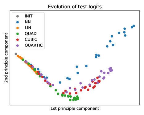
Figure 1: Function space dynamics of a 4-layer CNN under full training ( NN) and Taylorized training of order 1-4 ( linearized, quadratic, cubic, quartic). All models are trained on CIFAR-10 with the same initialization + optimization setup, and we plot the test logits on the trained models in the first 20 epochs. Each point is a 2D PCA embedding of the test logits of the corresponding model. Observe that Taylorized training becomes an increasingly better approximation of full NN training as we increase the expansion order $k$.

2 Preliminaries

We consider the supervised learning problem

$$\mathop{\rm minimize}~{}~{}L(\theta)=\mathbb{E}_{(x,y)\sim P}[\ell(f_{\theta}(x),y)],$$

where $x\in\mathbb{R}^{d}$ is the input, $y\in\mathcal{Y}$ is the label, $\ell:\mathbb{R}^{C}\times\mathcal{Y}\to\mathbb{R}$ is a convex loss function, $\theta\in\mathbb{R}^{p}$ is the learnable parameter, and $f_{\theta}:\mathbb{R}^{d}\to\mathbb{R}^{C}$ is the neural network that maps the input to the output (e.g. the prediction in a regression problem, or the vector of logits in a classification problem).

This paper focuses on the case where $f_{\theta}$ is a (deep) neural network. A standard feedforward neural network with $L$ layers is defined through $f_{\theta}(x)=h^{L}$, where $h^{0}=x^{0}=x$, and

$$h^{\ell+1}=W^{\ell+1}x^{\ell}+b^{\ell+1},~{}~{}~{}x^{\ell+1}=\sigma(h^{\ell+1})$$ (1)

for all $\ell\in{\left\{0,\dots,L-1\right\}}$, where $W^{\ell}\in\mathbb{R}^{d_{\ell}\times d_{\ell-1}}$ are weight matrices, $b^{\ell}\in\mathbb{R}^{d_{\ell}}$ are biases, and $\sigma:\mathbb{R}\to\mathbb{R}$ is an activation function (e.g. the ReLU) applied entry-wise. We will not describe other architectures in detail; for the purpose of describing our approach and empirical results, it suffices to think of $f_{\theta}$ as a general nonlinear function of the parameter $\theta$ (for a given input $x$.)

Once the architecture is chosen, it remains to define an initialization strategy and a learning rule.

Initialization and training

We will mostly consider the standard initialization (or variants of it such as Xavier Glorot & Bengio (2010) or Kaiming He et al. (2015)) in this paper, which for a feedforward network is defined as

$$\theta_{0}={\left\{(W^{\ell}_{0},b^{\ell}_{0})\right\}}_{\ell=1}^{L+1},~{}{\rm where}$$

$$W^{\ell}_{0,ij}\sim\mathsf{N}(0,1/d_{\ell})~{}~{}~{}{\rm and}~{}~{}~{}b^{\ell}_{0,i}\sim\mathsf{N}(0,1),$$

and can be similarly defined for convolutional and residual networks. This is in contrast with the NTK parameterization (Jacot et al., 2018), which encourages the weights to move significantly less.

We consider training the neural network via (stochastic) gradient descent:

$$\theta_{t+1}=\theta_{t}-\eta_{t}\nabla L(\theta_{t}).$$ (2)

We will refer to the above as full training of neural networks, so as to differentiate with various approximate training regimes to be introduced below.

3 Linearized Training and Its Limitations

We briefly review the theory of linearized training (Lee et al., 2019; Chizat et al., 2019) for explaining the training and generalization success of neural networks, and provide insights on its limitations.

3.1 Linearized training and Neural Tangent Kernels

The theory of linearized training begins with the observation that a neural network near init can be accurately approximated by a linearized network. Given an initialization $\theta_{0}$ and an arbitrary $\theta$ near $\theta_{0}$, we have that

$$f_{\theta}(x)=\underbrace{f_{\theta_{0}}(x)+\left\langle\nabla f_{\theta_{0}}(x),\theta-\theta_{0}\right\rangle}_{\mathrel{\mathop{:}}=f^{\rm lin}_{\theta}(x)}+o{\left(\left\|{\theta-\theta_{0}}\right\|\right)},$$

that is, the neural network $f_{\theta}$ is approximately equal to the linearized network $f^{\rm lin}_{\theta}$. Consequently, near $\theta_{0}$, the trajectory of minimizing $L(\theta)$ can be well approximated by the trajectory of linearized training, i.e. minimizing

$$L^{\rm lin}(\theta)\mathrel{\mathop{:}}=\mathbb{E}_{(x,y)\sim P}[\ell(f^{\rm lin}_{\theta}(x),y)],$$

which is a convex problem and enjoys convergence guarantees.

Furthermore, linearized training can approximate the entire trajectory of full training provided that we are in a certain linearized regime in which we use

• Small learning rate, so that $\theta$ stays in a small neighborhood of $\theta_{0}$ for any fixed amount of time;

• Over-parameterization, so that such a neighborhood gives a function space that is rich enough to contain a point $\theta$ so that $f^{\rm lin}_{\theta}$ can fit the entire training dataset.

As soon as we are in the above linearized regime, gradient descent is guaranteed to reach a global minimum  (Du et al., 2019; Allen-Zhu et al., 2019b; Zou et al., 2019). Further, as the width goes to infinity, due to randomness in the initialization $\theta_{0}$, the function space containing such linearized models goes to a statistical limit governed by the Neural Tangent Kernels (NTKs) Jacot et al. (2018), so that wide networks trained in this linearized regime generalize as well as a kernel method Arora et al. (2019a); Allen-Zhu et al. (2019a).

3.2 Unrealisticness of linearized training in practice

Our key concern about the theory of linearized training is that there are significant differences between training regimes in which the linearized approximation is accurate, and regimes in which neural nets typically attain their best performance in practice. More concretely,

1. Linearized training is a good approximation of full training under small learning rates in which each individual weight barely moves. However, neural networks typically attain their best test performance when using a large (initial) learning rate, in which the weights move significantly in a way not explained by linearized training Li et al. (2019a);

2. Linearized networks are powerful models on their own when the base architecture is over-parameterized, but can be rather poor when the network is of a practical size. Indeed, infinite-width linearized models such as CNTK achieve competitive performance on benchmark tasks Arora et al. (2019b; c), yet their finite-width counterparts often perform significantly worse  Lee et al. (2019); Chizat et al. (2019).

4 Taylorized Training

Towards closing this gap between linearized and full training, we propose to study Taylorized training, a principled extension of linearized training. Taylorized training involves training higher-order expansions of the neural network around the initialization. For any $k\geq 1$—assuming sufficient smoothness—we can Taylor expand $f_{\theta}$ to the $k$-th order as

$$f_{\theta}(x)=\underbrace{f_{\theta_{0}}(x)+\sum_{j=1}^{k}\frac{\nabla^{j}f_{\theta_{0}}(x)}{j!}[\theta-\theta_{0}]^{\otimes j}}_{\mathrel{\mathop{:}}=f^{(k)}_{\theta}(x)}+o{\left(\left\|{\theta-\theta_{0}}\right\|^{k}\right)},$$

where we have defined the $k$-th order Taylorized model $f^{(k)}_{\theta}(x)$. The Taylorized model $f^{(k)}_{\theta}$ reduces to the linearized model when $k=1$, and is a $k$-th order polynomial model for a general $k$, where the “features” are $\nabla^{j}f_{\theta_{0}}(x)\in\mathbb{R}^{C\times p^{\otimes j}}$ (which depend on the architecture $f$ and initialization $\theta_{0}$), and the “coefficients” are $(\theta-\theta_{0})^{\otimes j}$ for $j=1,\dots,k$.

Similar as linearized training, we define Taylorized training as the process (or trajectory) for training $f^{(k)}_{\theta}$ via gradient descent, starting from the initialization $\theta=\theta_{0}$. Concretely, the trajectory for $k$-th order Taylorized training will be denoted as $\theta^{(k)}_{t}$, where

$$\theta^{(k)}_{t+1}=\theta^{(k)}_{t}-\eta_{t}\nabla L^{(k)}(\theta^{(k)}_{t}),~{}~{}{\rm where}$$ (3)

$$L^{(k)}(\theta)\mathrel{\mathop{:}}=\mathbb{E}_{(x,y)\sim P}[\ell(f^{(k)}_{\theta}(x),y)].$$

Taylorized models arise from a similar principle as linearized models (Taylor expansion of the neural net), and gives increasingly better approximations of the neural network (at least locally) as we increase $k$. Further, higher-order Taylorized training ($k\geq 2$) are no longer convex problems, yet they model the non-convexity of full training in a mild way that is potentially amenable to theoretical analyses. Indeed, quadratic training ($k=2$) been shown to enjoy a nice optimization landscape and achieve better sample complexity than linearized training on learning certain simple functions Bai & Lee (2020). Higher-order training also has the potential to be understood through its polynomial structure and its connection to tensor decomposition problems Mondelli & Montanari (2019).

Implementation

Naively implementing Taylorization by directly computing higher-order derivative tensors of neural networks is prohibitive in both memory and time. Fortunately, Taylorized models can be efficiently implemented through a series of nested Jacobian-Vector Product operations (JVPs). Each JVP operation can be computed with the $\mathcal{R}$-operator algorithm of Pearlmutter (1994), which gives directional derivatives through arbitrary differentiable functions, and is the transpose of backpropagation.

For any function $f$ with parameters $\theta_{0}$, we denote its JVP with respect to the direction $\Delta\theta\mathrel{\mathop{:}}=\theta-\theta_{0}$ using the notation of Pearlmutter (1994) by

$$\mathcal{R}_{\Delta\theta}(f_{\theta_{0}}(x))\mathrel{\mathop{:}}=\frac{\partial}{\partial r}f_{(\theta_{0}+r\Delta\theta)}(x)|_{r=0}.$$ (4)

The $k$-th order Taylorized model can be computed as

$$f^{(k)}_{\theta}(x)=f_{\theta_{0}}(x)+\sum_{j=1}^{k}\frac{\mathcal{R}^{j}_{\Delta\theta}(f_{\theta_{0}}(x))}{j!},$$ (5)

where $\mathcal{R}^{j}$ is the $j$-times nested evaluation of the $\mathcal{R}$-operator.

Our implementation uses Jax Bradbury et al. (2018) and neural_tangents Novak et al. (2020) which has built-in support for Taylorizing any function to an arbitrary order based on nested JVP operations.

5 Experiments

Name	Architecture	Params	Train For	Batch	Accuracy	Opt	Rate	Grad Clip	LR Decay Schedule
CNNTHIN	CNN-4-128	447K	200 epochs	256	81.6%	SGD	0.1	5.0	10x drop at 100, 150 epochs
CNNTHICK	CNN-4-512	7.10M	160 epochs	64	85.9%	SGD	0.1	5.0	10x drop at 80, 120 epochs
WRNTHIN	WideResNet-16-4-128	3.22M	200 epochs	256	88.1%	SGD	1e-1.5	10.0	10x drop at 100, 150 epochs
WRNTHICK	WideResNet-16-8-256	12.84M	160 epochs	64	91.7%	SGD	1e-1.5	10.0	10x drop at 80, 120 epochs

Table 1: Our architectures and training setups. CNN-$L$-$C$ stands for a CNN with depth $L$ and $C$ channels per layer. WideResNet-$L$-$k$-$C$ stands for a WideResNet with depth $L$, widening factor $k$, and $C$ channels in the first convolutional layer.

We experiment with Taylorized training on convolutional and residual networks for the image classification task on CIFAR-10.

5.1 Basic setup

We choose four representative architectures for the image classification task: two CNNs with 4 layers + Global Average Pooling (GAP) with width ${\left\{128,512\right\}}$, and two WideResNets Zagoruyko & Komodakis (2016) with depth 16 and different widths as well. All networks use standard parameterization and are trained with the cross-entropy loss. We optimize the training loss using SGD with a large initial learning rate + learning rate decay.

For each architecture, the initial learning rate was tuned within ${\left\{10^{-2},10^{-1.5},10^{-1},10^{-0.5}\right\}}$ and chosen to be the largest learning rate under which the full neural network can stably train (i.e. has a smoothly decreasing training loss). We use standard data augmentation (random crop, flip, and standardize) as a optimization-independent way for improving generalization. Detailed training settings for each architecture are summarized in Table 1.

Methodology

For each architecture, we train Taylorized models of order $k\in{\left\{1,2,3,4\right\}}$ (referred to as {linearized, quadratic, cubic, quartic} models) from the same initialization as full training using the exact same optimization setting (including learning rate decay, gradient clipping, minibatching, and data augmentation noise). This allows us to eliminate the effects of optimization setup and randomness, and examine the agreement between Taylorized and full training in identical settings.

5.2 Approximation power of Taylorized training

We examine the approximation power of Taylorized training through comparing Taylorized training of different orders in terms of both the training trajectory and the test performance.

Metrics

We monitor the training loss and test accuracy for both full and Taylorized training. We also evaluate the approximation error between Taylorized and full training quantitatively through the following similarity metrics between models:

• Cosine similarity in the parameter space, defined as

  $${\rm cos\_param}_{t}\mathrel{\mathop{:}}=\frac{\left\langle\theta^{(k)}_{t}-\theta_{0},\theta_{t}-\theta_{0}\right\rangle}{\big{\|}\theta^{(k)}_{t}-\theta_{0}\big{\|}\big{\|}\theta_{t}-\theta_{0}\big{\|}},$$

  where (recall (3) and (2)) $\theta^{(k)}_{t}$ and $\theta_{t}$ denote the parameters in $k$-th order Taylorized training and full training, and $\theta_{0}$ is their common initialization.

• Cosine similarity in the function space, defined as

  $${\rm cos\_func}_{t}\mathrel{\mathop{:}}=\frac{\left\langle f^{(k)}_{\theta^{(k)}_{t}}-f_{\theta_{0}},f_{\theta_{t}}-f_{\theta_{0}}\right\rangle}{\big{\|}f^{(k)}_{\theta^{(k)}_{t}}-f_{\theta_{0}}\big{\|}\big{\|}f_{\theta_{t}}-f_{\theta_{0}}\big{\|}},$$

  where we have overloaded the notation $f\in\mathbb{R}^{C\times n_{\rm test}}$ (and similarly $f^{(k)}$) to denote the output (logits) of a model on the test dataset.

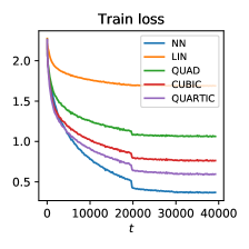
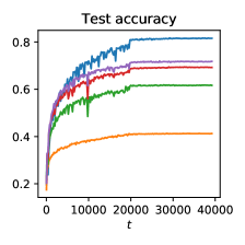
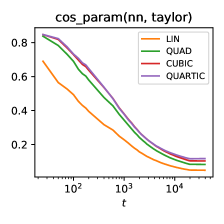
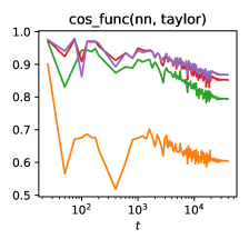
Figure 2: $k$-th order Taylorized training approximates full training increasingly better with $k$ on the CNNTHIN model. Training statistics are plotted for { full, linearized, quadratic, cubic, quartic} models. Left to right: (1) training loss; (2) test accuracy; (3) cosine similarity between Taylorized and full training in the parameter space; (4) cosine similarity between Taylorized and full training in the function (logit) space. All models are trained on CIFAR-10 for 39200 steps, and a 10x learning rate decay happened at step {19600, 29400}.

Architecture	CNNTHIN	CNNTHICK	WRNTHIN	WRNTHICK
Linearized ($k=1$)	41.3%	49.0%	50.2%	55.3%
Quadratic ($k=2$)	61.6%	70.1%	65.8%	71.7%
Cubic ($k=3$)	69.3%	75.3%	72.6%	76.9%
Quartic ($k=4$)	71.8%	76.2%	75.6%	78.7%
Full network	81.6%	85.9%	88.1%	91.7%

Table 2: Final test accuracy on CIFAR-10 for Taylorized models trained under the same optimization setup as full neural nets. Details about the architectures and their training setups can be found in Table 1.

Results

Figure 2 plots training and approximation metrics for full and Taylorized training on the CNNTHIN model. Observe that Taylorized models are much better approximators than linearized models in both the parameter space and the function space—both cosine similarity curves shift up as we increase $k$ from 1 to 4. Further, for the cubic and quartic models, the cosine similarity in the logit space stays above 0.8 over the entire training trajectory (which includes both weakly and strongly trained models), suggesting a fine agreement between higher-order Taylorized training and full training. Results for {CNNTHICK, WRNTHIN, WRNTHICK} are qualitatively similar and are provided in Appendix B.1.

We further report the final test performance of the Taylorized models on all architectures in Table 2. We observe that

1. Taylorized models can indeed close the performance gap between linearized and full training: linearized models are typically 30%-40% worse than fully trained networks, whereas quartic (4th order Taylorized) models are within {10%, 13%} of a fully trained network on {CNNs, WideResNets}.

2. All Taylorized models can benifit from increasing the width (from CNNTHIN to CNNTHICK, and WRNTHIN to WRNTHICK), but the performance of higher-order models ($k=3,4$) are generally less sensitive to width than lower-order models ($k=1,2$), suggesting their realisticness for explaining the training behavior of practically sized finite-width networks.

On finite- vs. infinite-width linearized models

We emphasize that the performance of our baseline linearized models in Table 2 (40%-55%) is at finite width, and is thus not directly comparable to existing results on infinite-width linearized models such as CNTK Arora et al. (2019b). It is possible to achieve stronger results with finite-width linearized networks by using the NTK parameterization, which more closely resembles the infinite width limit. However, full neural net training with this re-parameterization results in significantly weakened performance, suggesting its unrealisticness. The best documented test accuracy of a finite-width linearized network on CIFAR-10 is $\sim$65% Lee et al. (2019), and due to the NTK parameterization, the neural network trained under these same settings only reached $\sim$70%. In contrast, our best higher order models can approach 80%, and are trained under realistic settings where a neural network can reach over 90%.

5.3 Agreement on layer movements

Layer importance, i.e. the contribution and importance of each layer in a well-trained (deep) network, has been identified as a useful concept towards building an architecture-dependent understanding on neural network training Zhang et al. (2019). Here we demonstrate that higher-order Taylorized training has the potential to lead to better understandings on the layer importance in full training.

Method and result

We examine layer movements, i.e. the distances each layer has travelled along training, and illustrate it on both full and Taylorized training. In Figure 3, we plot the layer movements on the CNNTHIN and WRNTHIN models. Compared with linearized training, quartic training agrees with full training much better in the shape of the layer movement curve, both at an early stage and at convergence. Furthermore, comparing the layer movement curves between the 10th epoch and at convergence, quartic training seems to be able to adjust the shape of the movement curve much better than linearized training.

Intriguing results about layer importance has also been (implicitly) shown in the study of infinite-width linearized models (i.e. NTK type kernel methods). For example, it has been observed that the CNN-GP kernel (which corresponds to training the top layer only) has consistently better generalization performance than the CNTK kernel (which corresponds to training all the layer) Li et al. (2019b). In other words, when training an extremely wide convolutional net on a finite dataset, training the last layer only gives a better generalization performance (i.e. a better implicit bias); existing theoretical work on linearized training fall short of understanding layer importance in these settings. We believe Taylorized training can serve as an (at least empirically) useful tool towards understanding layer importance.

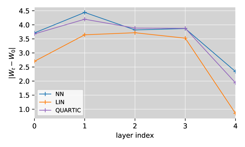
(a) CNNTHIN at 10 epochs

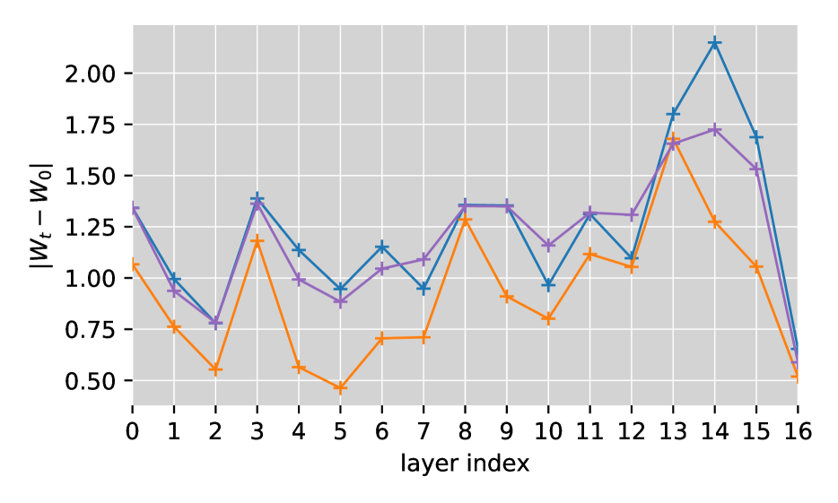
(b) WRNSMALL at 10 epochs

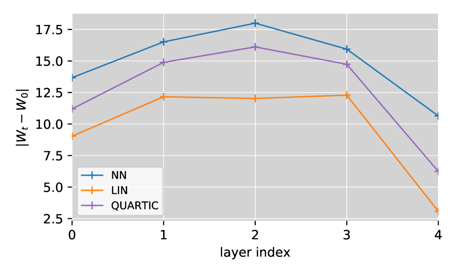
(c) CNNTHIN at convergence

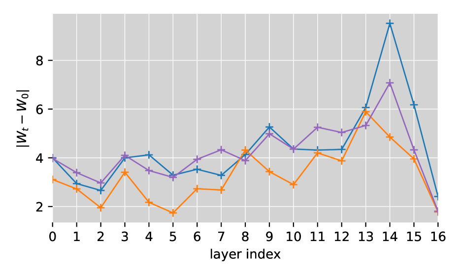
(d) WRNSMALL at convergence

Figure 3: Layer movement of full NN, linearized, and quartic models. Compared with linearized training, quartic (4th order) Taylorized training agrees with the full neural network much better in terms of layer movement, both at the initial stage and at convergence.

6 Theoretical Results

We provide a theoretical analysis on the distance between the trajectories of Taylorized training and full training on wide neural networks.

Problem Setup

We consider training a wide two-layer neural network with width $m$ and the NTK parameterization:

$$f_{W}(x)=\frac{1}{\sqrt{m}}\sum_{r=1}^{m}a_{r}\sigma(w_{r}^{\top}x),$$ (6)

where $x\in\mathbb{R}^{d}$ is the input satisfying $\left\|{x}\right\|_{2}=1$, ${\left\{w_{r}\right\}}_{r\in[m]}\subset\mathbb{R}^{d}$ are the neurons, ${\left\{a_{r}\right\}}\subset\mathbb{R}$ are the top-layer coefficients, and $\sigma:\mathbb{R}\to\mathbb{R}$ is a smooth activation function. We set ${\left\{a_{r}\right\}}$ fixed and only train ${\left\{w_{r}\right\}}$, so that the learnable parameter of the problem is the weight matrix $W=[w_{1},\dots,w_{m}]\in\mathbb{R}^{d\times m}$.

We initialize $(a,W)=(a_{0},W_{0})$ randomly according to the standard initialization, that is,

$$a_{r}\equiv a_{r,0}\sim{\rm Unif}{\left\{\pm 1\right\}}~{}~{}~{}{\rm and}~{}~{}~{}w_{r,0}\sim\mathsf{N}(0,I_{d}).$$

We consider the regression task over a finite dataset $\mathcal{D}={\left\{(x_{i},y_{i})\in\mathbb{R}^{d}\times\mathbb{R}:i\in[n]\right\}}$ with squared loss

$$L(W)=\frac{1}{2}\mathbb{E}_{(x,y)\sim\mathcal{D}}{\left[(y-f_{W}(x))^{2}\right]},$$

and train $W$ via gradient flow (i.e. continuous time gradient descent) with “step-size” $\eta_{0}$:

$$\dot{W}_{t}=-\eta_{0}\nabla L(W_{t}).$$ (7)

Taylorized training

We compare the full training dynamics (7) with the corresponding Taylorized training dynamics. The $k$-th order Taylorized model for the neural network (6), denoted as $f^{(k)}_{W}$, has the form

$$f^{(k)}_{W}(x)=\frac{1}{\sqrt{m}}\sum_{r=1}^{m}a_{r}\sum_{j=0}^{k}\frac{\sigma^{(j)}(w_{r,0}^{\top}x)}{j!}{\left[(w_{r}-w_{r,0})^{\top}x\right]}^{j}.$$

The Taylorized training dynamics can be described as

$$\dot{W}^{(k)}_{t}=-\eta_{0}\nabla L^{(k)}(W^{(k)}_{t}),~{}~{}~{}{\rm where}$$ (8)

$$L^{(k)}(W)=\frac{1}{2}\mathbb{E}_{(x,y)\sim\mathcal{D}}{\left[(y-f^{(k)}_{W}(x))^{2}\right]},$$

starting at the same initialization $W^{(k)}_{0}=W_{0}$.

We now present our main theoretical result which gives bounds on the agreement between $k$-th order Taylorized training and full training on wide neural networks.

Theorem 1 (Agreement between Taylorized and full training: informal version).

There exists a suitable step-size $\eta_{0}$ such that for any fixed $t_{0}>0$ and all suffiicently large $m$, with high probability over the random initialization, full training (7) and Taylorized training (8) are coupled in both the parameter space and the function space:

$$\sup_{t\leq t_{0}}\left\|{W_{t}-W^{(k)}_{t}}\right\|_{\sf Fr}\leq O(m^{-k/2}),$$

$$\sup_{t\leq t_{0}}{\left|f_{W_{t}}(x)-f^{(k)}_{W^{(k)}_{t}}(x)\right|}\leq O(m^{-k/2})~{}~{}\textrm{for all}~{}\left\|{x}\right\|_{2}=1.$$

Theorem 1 extends existing results which state that linearized training approximates full training with an error bound $O(1/\sqrt{m})$ in the function space Lee et al. (2019); Chizat et al. (2019), showing that higher-order Taylorized training enjoys a stronger approximation bound $O(m^{-k/2})$. Such a bound corroborates our experimental finding that Taylorized training are increasingly better approximations of full training as we increase $k$. We defer the formal statement of Theorem 1 and its proof to Appendix A.

We emphasize that Theorem 1 is still only mostly relevant for explaining the initial stage rather than the entire trajectory for full training in practice, due to the fact that the result holds for gradient flow which only simulates gradient descent with an infinitesimally small learning rate. We believe it is an interesting open direction how to prove the coupling between neural networks and the $k$-th order Taylorized training under large learning rates.

7 Related Work

Here we review some additional related work.

Neural networks, linearized training, and kernels

The connection between wide neural networks and kernel methods has first been identified in Neal (1996). A fast-growing body of recent work has studied the interplay between wide neural networks, linearized models, and their infinite-width limits governed by either the Gaussian Process (GP) kernel (corresponding to training the top linear layer only) Daniely (2017); Lee et al. (2018); Matthews et al. (2018) or the Neural Tangent Kernel (corresponding to training all the layers) Jacot et al. (2018). By exploiting such an interplay, it has been shown that gradient descent on overparameterized neural nets can reach global minima Jacot et al. (2018); Du et al. (2018; 2019); Allen-Zhu et al. (2019b); Zou et al. (2019); Lee et al. (2019), and generalize as well as a kernel method Li & Liang (2018); Arora et al. (2019a); Cao & Gu (2019).

NTK-based and NTK-inspired learning algorithms

Inspired by the connection between neural nets and kernel methods, algorithms for computing the exact (limiting) GP / NTK kernels efficiently has been proposed Arora et al. (2019b); Lee et al. (2019); Novak et al. (2020); Yang (2019) and shown to yield state-of-the-art kernel-based algorithms on benchmark learning tasks Arora et al. (2019b); Li et al. (2019b); Arora et al. (2019c). The connection between neural nets and kernels have further been used in designing algorithms for general machine learning use cases such as multi-task learning Mu et al. (2020) and protecting against noisy labels Hu et al. (2020).

Limitations of linearized training

The performance gap between linearized and fully trained networks has been empirically observed in Arora et al. (2019b); Lee et al. (2019); Chizat et al. (2019). On the theoretical end, the sample complexity gap between linearized training and full training has been shown in Wei et al. (2019); Ghorbani et al. (2019a); Allen-Zhu & Li (2019); Yehudai & Shamir (2019) under specific data distributions and architectures.

Provable training beyond linearization

Allen-Zhu et al. (2019a); Bai & Lee (2020) show that wide neural nets can couple with quadratic models with provably nice optimization landscapes and better generalization than the NTKs, and Bai & Lee (2020) furthers show the sample complexity benefit of $k$-th order models for all $k$.  Li et al. (2019a) show that a large initial learning rate + learning rate decay generalizes better than a small learning rate for learning a two-layer network on a specific toy data distribution.

An parallel line of work studies over-parameterized neural net training in the mean-field limit, in which the training dynamics can be characterized as a PDE over the distribution of weights Mei et al. (2018); Chizat & Bach (2018); Rotskoff & Vanden-Eijnden (2018); Sirignano & Spiliopoulos (2018). Unlike the NTK regime, the mean-field regime moves weights significantly, though the inductive bias (what function it converges to) and generalization power there is less clear.

8 Conclusion

In this paper, we introduced and studied Taylorized training. We demonstrated experimentally the potential of Taylorized training in understanding full neural network training, by showing its advantage in terms of approximation in both weight and function space, training and test performance, and other empirical properties such as layer movements. We also provided a preliminary theoretical analysis on the approximation power of Taylorized training.

We believe Taylorized training can serve as a useful tool towards studying the theory of deep learning and open many interesting future directions. For example, can we prove the coupling between full and Taylorized training with large learning rates? How well does Taylorized training approximate full training as $k$ approaches infinity? Following up on our layer movement experiments, it would also be interesting use Taylorized training to study the properties of neural network architectures or initializations.

Appendix A Proof of Theorem 1

A.1 Formal statement of Theorem 1

We first collect notation and state our assumptions. Recall that our two-layer neural network is defined as

$$f_{W}(x)=\frac{1}{\sqrt{m}}\sum_{r=1}^{m}a_{r}\sigma(w_{r}^{\top}x),$$

and its $k$-th order Taylorized model is

$$f^{(k)}_{W}(x)=\frac{1}{\sqrt{m}}\sum_{r=1}^{m}a_{r}\sum_{j=0}^{k}\frac{\sigma^{(j)}(w_{r,0}^{\top}x)}{j!}{\left[(w_{r}-w_{r,0})^{\top}x\right]}^{j}.$$ (9)

Let $\mathcal{X}\in\mathbb{R}^{d\times n}$ and $\mathcal{Y}\in\mathbb{R}^{n}$ denote inputs and labels of the training dataset. For any weight matrix $W\in\mathbb{R}^{d\times m}$ we let

$$f(W)=f(W;\mathcal{X})\mathrel{\mathop{:}}=\begin{bmatrix}f_{W}(x_{1})\\ \vdots\\ f_{W}(x_{n})\end{bmatrix}\in\mathbb{R}^{n},~{}~{}~{} f^{(k)}(W)=f^{(k)}(W;\mathcal{X})\mathrel{\mathop{:}}=\begin{bmatrix}f^{(k)}_{W}(x_{1})\\ \vdots\\ f^{(k)}_{W}(x_{n})\end{bmatrix}\in\mathbb{R}^{n},$$

$$g(W)=f(W)-\mathcal{Y}\in\mathbb{R}^{n},~{}~{}~{} g^{(k)}(W)=f^{(k)}(W)-\mathcal{Y}\in\mathbb{R}^{n},$$

$$f_{t}\mathrel{\mathop{:}}=f(W_{t}),~{}~{}~{} f^{(k)}_{t}\mathrel{\mathop{:}}=f^{(k)}(W^{(k)}_{t}),$$

$$g_{t}\mathrel{\mathop{:}}=g(W_{t}),~{}~{}~{} g^{(k)}_{t}\mathrel{\mathop{:}}=g^{(k)}(W^{(k)}_{t}),$$

$$J(W)\mathrel{\mathop{:}}=\begin{bmatrix}\nabla f_{W}(x_{1})\\ \vdots\\ \nabla f_{W}(x_{n})\end{bmatrix}\in\mathbb{R}^{n\times dm},~{}~{}~{} J^{(k)}(W)\mathrel{\mathop{:}}=\begin{bmatrix}\nabla f^{(k)}_{W}(x_{1})\\ \vdots\\ \nabla f^{(k)}_{W}(x_{n})\end{bmatrix}\in\mathbb{R}^{n\times dm}.$$

With this notation, the loss functions can be written as $L(W)=\left\|{g(W)}\right\|^{2}$ and $L^{(k)}(W)=\left\|{g^{(k)}(W)}\right\|^{2}$, and the training dynamics (full and Taylorized) can be written as

$$\dot{W}_{t}=-\eta_{0}\cdot J(W_{t})^{\top}g_{t},\qquad\dot{g}_{t}=-\eta_{0}\cdot J(W_{t})J(W_{t})^{\top}g_{t},$$

$$\dot{W}^{(k)}_{t}=-\eta_{0}\cdot J^{(k)}(W^{(k)}_{t})^{\top}g^{(k)}_{t},\qquad\dot{g}^{(k)}_{t}=-\eta_{0}\cdot J^{(k)}(W^{(k)}_{t})J^{(k)}(W^{(k)}_{t})^{\top}g^{(k)}_{t}.$$

We now state our assumptions.

Assumption A (Full-rankness of analytic NTK).

The analytic NTK $\Theta\in\mathbb{R}^{n\times n}$ on the training dataset, defined as

$$\Theta\mathrel{\mathop{:}}=\lim_{m\to\infty}J(W_{0})J(W_{0})^{\top}~{}~{}~{}\textrm{in probability},$$

is full rank and satisfies $\lambda_{\min}(\Theta)\geq\lambda_{\min}$ for some $\lambda_{\min}>0$.

Assumption B (Smooth activation).

The activation function $\sigma:\mathbb{R}\to\mathbb{R}$ is $C^{k}$ and has a bounded Lipschitz derivative: there exists a constant $C>0$ such that

$$\sup_{t\in\mathbb{R}}{\left|\sigma^{\prime}(t)\right|}\leq C~{}~{}~{}{\rm and}~{}~{}~{}\sup_{t\neq t^{\prime}\in\mathbb{R}}{\left|\frac{\sigma^{\prime}(t)-\sigma^{\prime}(t^{\prime})}{t-t^{\prime}}\right|}\leq C.$$

Further, $\sigma^{\prime}$ has a Lipschitz $k$-th derivative: $t\mapsto\sigma^{(k)}(t)$ is $L$-Lipschitz for some constant $L>0$.

Throughout the rest of this section, we assume the above assumptions hold. We are now in position to formally state our main theorem.

Theorem 2 (Approximation error of Taylorized training; formal version of Theorem 1).

There exists a suitable step-size choice $\eta_{0}>0$ such that the following is true: for any fixed $t_{0}>0$ and all sufficiently large $m$, with high probability over the random initialization, full training (7) and Taylorized training (8) are coupled in both the parameter space and the function space:

$$\sup_{t\leq t_{0}}\left\|{W_{t}-W^{(k)}_{t}}\right\|_{\sf Fr}\leq O(m^{-k/2}),$$

$$\sup_{t\leq t_{0}}{\left|f_{W_{t}}(x)-f^{(k)}_{W^{(k)}_{t}}(x)\right|}\leq O(m^{-k/2})~{}~{}\textrm{for all}~{}\left\|{x}\right\|_{2}=1.$$

Remark on extending to entire trajectory

Compared with the existing result on linearized training (Lee et al., 2019, Theorem H.1), our Theorem 2 only shows the approximation for a fixed time horizon $t\in[0,t_{0}]$ instead of the entire trajectory $t\in[0,\infty)$. Technically, this is due to that the linearized result uses a more careful Gronwall type argument which relies on the fact that the kernel does not change, which ceases to hold here. It would be a compelling question if we could show the approximation result for higher-order Taylorized training for the entire trajectory.

A.2 Proof of Theorem 2

Throughout the proof, we let $K$ be a constant that does not depend on $m$, but can depend on other problem parameters and can vary from line to line. We will also denote

$$\sigma^{(k)}_{r,i}(t)\mathrel{\mathop{:}}=\sum_{j=0}^{k}\frac{\sigma^{(j)}(w_{r,0}^{\top}x_{i})}{j!}{\left[t-w_{r,0}^{\top}x_{i}\right]}^{j},$$ (10)

so that the Taylorized model can be essentially thought of as a two-layer neural network with the (data- and neuron-dependent) activation functions $\sigma^{(k)}_{r,i}$.

We first present some known results about the full training trajectory $W_{t}$, adapted from (Lee et al., 2019, Appendix G).

Lemma 3 (Basic properties of full training).

Under Assumptions A, B, the followings hold:

1. $J$ is locally bounded and Lipschitz: For any absolute constant $C>0$ there exists a constant $K>0$ such that for sufficiently large $m$, with high probability (over the random initialization $W_{0}$) we have

   $$\left\|{J(W)-J(\widetilde{W})}\right\|_{\sf Fr}\leq K\left\|{W-\widetilde{W}}\right\|_{\sf Fr}~{}~{}~{}{\rm and}$$

   $$\left\|{J(W)}\right\|_{\sf Fr}\leq K$$

   for any $W,\widetilde{W}\in\mathsf{B}(W_{0},C)$, where $\mathsf{B}(W_{0},R)\mathrel{\mathop{:}}={\left\{W\in\mathbb{R}^{d\times m}:\left\|{W-W_{0}}\right\|_{\sf Fr}\leq R\right\}}$ denotes a Frobenius norm ball.

2. Boundedness of gradient flow: there exists an absolute $R_{0}>0$ such that with high probability for sufficiently large $m$ and a suitable step-size choice $\eta_{0}$ (independent of $m$), we have for all $t>0$ that

   $$\left\|{g_{t}}\right\|_{2}\leq\exp(-\eta_{0}\lambda_{\min}t/3)R_{0},$$

   $$\left\|{W_{t}-W_{0}}\right\|_{\sf Fr}\leq\frac{KR_{0}}{\lambda_{\min}}{\left(1-\exp(-\eta_{0}\lambda_{\min}t/3)\right)}m^{-1/2},$$

   $$\sup_{t\geq 0}\left\|{\widehat{\Theta}_{0}-\widehat{\Theta}_{t}}\right\|_{\sf Fr}\leq\frac{K^{3}R_{0}}{\lambda_{\min}}m^{-1/2}.$$

Lemma 4 (Properties of Taylorized training).

Lemma 3 also holds if we replace full training with $k$-th order Taylorized training. More concretely, we have

1. $J^{(k)}$ is locally bounded and Lipschitz: For any absolute constant $C>0$ there exists a constant $K>0$ such that for sufficiently large $m$, with high probability (over the random initialization $W_{0}$) we have

   $$\left\|{J^{(k)}(W)-J^{(k)}(\widetilde{W})}\right\|_{\sf Fr}\leq K\left\|{W-\widetilde{W}}\right\|_{\sf Fr}~{}~{}~{}{\rm and}$$

   $$\left\|{J^{(k)}(W)}\right\|_{\sf Fr}\leq K$$

   for any $W,\widetilde{W}\in\mathsf{B}(W_{0},C)$, where $\mathsf{B}(W_{0},R)\mathrel{\mathop{:}}={\left\{W\in\mathbb{R}^{d\times m}:\left\|{W-W_{0}}\right\|_{\sf Fr}\leq R\right\}}$ denotes a Frobenius norm ball.

2. Boundedness of gradient flow: there exists an absolute $R_{0}>0$ such that with high probability for sufficiently large $m$ and a suitable step-size choice $\eta_{0}$ (independent of $m$), we have for all $t>0$ that

   $$\left\|{g^{(k)}_{t}}\right\|_{2}\leq\exp(-\eta_{0}\lambda_{\min}t/3)R_{0},$$

   $$\left\|{W^{(k)}_{t}-W_{0}}\right\|_{\sf Fr}\leq\frac{KR_{0}}{\lambda_{\min}}{\left(1-\exp(-\eta_{0}\lambda_{\min}t/3)\right)}m^{-1/2},$$

   $$\sup_{t\geq 0}\left\|{\widehat{\Theta}_{0}-\widehat{\Theta}^{(k)}_{t}}\right\|_{\sf Fr}\leq\frac{K^{3}R_{0}}{\lambda_{\min}}m^{-1/2}.$$

Proof.

1. Rewrite the $k$-th order Taylorized model (9) as

   $$f^{(k)}_{W}(x_{i})=\frac{1}{\sqrt{m}}\sum_{r=1}^{m}a_{r}\sigma_{r,i}^{(k)}(w_{r}^{\top}x_{i}),$$ (11)

   where we have used the definition of the “Taylorized” activation function $\sigma^{(k)}_{r,i}$ in (10).

   Our goal here is to show that $J^{(k)}$ is $K$-bounded and $K$-Lipschitz for some absolute constant $K$. By Lemma 3, it suffices to show the same for $J-J^{(k)}$, as we already have the result for the original Jacobian $J$. Let $W\in\mathsf{B}(W_{0},C)$, we have

   $$\quad\left\|{J(W)-J^{(k)}(W)}\right\|_{\sf Fr}^{2}=\sum_{i=1}^{n}\frac{1}{m}\sum_{r=1}^{m}{\left(\sigma^{\prime}(w_{r}^{\top}x_{i})-[\sigma^{(k)}]^{\prime}(w_{r}^{\top}x_{i})\right)}^{2}$$ (12)

   $$\stackrel{{\scriptstyle(i)}}{{\leq}}\sum_{i=1}^{n}\frac{1}{m}\sum_{r=1}^{m}{\left(\frac{L}{k!}\right)}^{2}{\left(w_{r}^{\top}x_{i}-w_{r,0}^{\top}x_{i}\right)}^{2k}$$

   $$\leq\frac{K}{m}\sum_{r=1}^{m}\left\|{w_{r}-w_{r,0}}\right\|_{2}^{2k}\leq\frac{K}{m}{\left(\sum_{r=1}^{m}\left\|{w_{r}-w_{r,0}}\right\|_{2}^{2}\right)}^{k}\leq KC^{k}/m\leq K.$$

   Above, (i) uses the $k$-th order smoothness of $\sigma$. This shows the boundedness of $J-J^{(k)}$.

   A similar argument can be done for the Lipschitzness of $J-J^{(k)}$, where the second-to-last expression is replaced by $\sum_{r\leq m}\left\|{w_{r}-w_{r,0}}\right\|_{2}^{2(k-1)}$, from which the same argument goes through as $2(k-1)\geq 2$ whenever $k\geq 2$, and for $k=1$ the sum is bounded by $K/m\cdot m=K$.

2. This is a direct corollary of part (a), as we can view the Taylorized network as an architecture on its own, which has the same NTK as $f$ at init (so the non-degeneracy of the NTK also holds), and has a locally bounded Lipschitz Jacobian. Repeating the argument of (Lee et al., 2019, Theorem G.2) gives the results.

∎

Lemma 5 (Bounding invididual weight movements in $W_{t}$ and $W^{(k)}_{t}$).

Under the same settings as Lemma 3 and 4, we have

$$\left\{\begin{aligned} &\max_{r\in[m]}\left\|{w_{r,t}-w_{r,0}}\right\|_{2}\leq\frac{KR_{0}}{\lambda_{\min}}(1-e^{-\eta_{0}\lambda_{\min}t/3})m^{-1/2},\\ &\max_{r\in[m]}\left\|{w^{(k)}_{r,t}-w_{r,0}}\right\|_{2}\leq\frac{KR_{0}}{\lambda_{\min}}(1-e^{-\eta_{0}\lambda_{\min}t/3})m^{-1/2}.\end{aligned}\right.$$ (13)

Consequently, we have for $\widetilde{W}_{t}\in{\left\{W_{t},W^{(k)}_{t}\right\}}$ that

$$\left\|{J(\widetilde{W}_{t})-J^{(k)}(\widetilde{W}_{t})}\right\|_{\sf Fr}\leq{\left(\frac{KR_{0}}{\lambda_{\min}}\right)}^{k}{\left(1-\exp(-\eta_{0}\lambda_{\min}t/3)\right)}^{k}m^{-k/2}.$$

Proof.

We first show the bound for $\left\|{w_{r,t}-w_{r,0}}\right\|_{2}$, and the bound for $\left\|{w^{(k)}_{r,t}-w_{r,0}}\right\|_{2}$ follows similarly. We have

$$\frac{d}{dt}\left\|{w_{r,t}-w_{r,0}}\right\|_{2}\leq\left\|{\frac{d}{dt}w_{r,t}}\right\|_{2}\leq\eta_{0}\left\|{J_{w_{r}}(W_{t})^{\top}g_{t}}\right\|_{2}\leq\eta_{0}\cdot\left\|{J_{w_{r}}(W_{t})}\right\|_{\sf Fr}\left\|{g_{t}}\right\|_{2}.$$

Note that

$$\left\|{J_{w_{r}}(W_{t})}\right\|_{\sf Fr}^{2}=\frac{1}{m}\sum_{i=1}^{n}\sigma^{\prime}(w_{r,t}^{\top}x_{i})^{2}\left\|{x_{i}}\right\|_{2}^{2}\leq\frac{1}{m}\cdot C^{2}=C^{2}/m.$$

due to the boundedness of $\sigma^{\prime}$, and $\left\|{g_{t}}\right\|_{2}\leq\exp(-\eta_{0}\lambda_{\min}t/3)R_{0}$ by Lemma 3(b), so we have

$$\quad\frac{d}{dt}\left\|{w_{r,t}-w_{r,0}}\right\|_{2}\leq\eta_{0}\left\|{J_{w_{r}}(W_{t})}\right\|_{\sf Fr}\left\|{g_{t}}\right\|_{2}$$

$$\leq\eta_{0}\cdot K/\sqrt{m}\cdot\exp(-\eta_{0}\lambda_{\min}t/3)R_{0}=K\eta_{0}R_{0}\exp(-\eta_{0}\lambda_{\min}t/3)m^{-1/2},$$

integrating which (and noticing the initial condition $\left\|{w_{r,t}-w_{r,0}}\right\|_{2}|_{t=0}=0$) yields that

$$\left\|{w_{r,t}-w_{r,0}}\right\|_{2}\leq\frac{3KR_{0}}{\lambda_{\min}}{\left(1-\exp(-\eta_{0}\lambda_{\min}t/3)\right)}m^{-1/2}.$$

We now show the bound on $\left\|{J-J^{(k)}}\right\|_{\sf Fr}$, again focusing on the case $\widetilde{W}_{t}\equiv W_{t}$ (and the case $\widetilde{W}_{t}\equiv W^{(k)}_{t}$ follows similarly). By (12), we have

$$\quad\left\|{J(W_{t})-J^{(k)}(W_{t})}\right\|_{\sf Fr}^{2}\leq\frac{K}{m}\sum_{r=1}^{m}\left\|{w_{r}-w_{r,0}}\right\|_{2}^{2k}\leq\frac{1}{m}\sum_{r=1}^{m}{\left(\frac{KR_{0}}{\lambda_{\min}}\right)}^{2k}\cdot(1-\exp(-\eta_{0}\lambda_{\min}t/3))^{2k}m^{-k}$$

$$={\left(\frac{KR_{0}}{\lambda_{\min}}\right)}^{2k}\cdot(1-\exp(-\eta_{0}\lambda_{\min}t/3))^{2k}m^{-k}.$$

Taking the square root gives the desired result. ∎

We are now in position to prove the main theorem.

Proof of Theorem 2     Step 1. We first bound the rate of change of $\left\|{W_{t}-W^{(k)}_{t}}\right\|_{\sf Fr}$. We have

$$\quad\frac{d}{dt}\left\|{W_{t}-W^{(k)}_{t}}\right\|_{\sf Fr}\leq\left\|{\frac{d}{dt}(W_{t}-W^{(k)}_{t})}\right\|_{\sf Fr}\leq\eta_{0}\left\|{J(W_{t})^{\top}g_{t}-J^{(k)}(W^{(k)}_{t})^{\top}g^{(k)}_{t}}\right\|_{\sf Fr}$$

$$\leq\underbrace{\eta_{0}\left\|{J(W_{t})-J^{(k)}(W_{t})}\right\|_{\sf Fr}\cdot\left\|{g_{t}}\right\|_{2}}_{\rm I}+\underbrace{\eta_{0}\left\|{J^{(k)}(W_{t})-J^{(k)}(W^{(k)}_{t})}\right\|_{\sf Fr}\cdot\left\|{g_{t}}\right\|_{2}}_{\rm II}+\underbrace{\eta_{0}\left\|{J^{(k)}(W^{(k)}_{t})}\right\|_{\sf Fr}\cdot\left\|{g_{t}-g^{(k)}_{t}}\right\|_{2}}_{\rm III}.$$

For term I, applying Lemma 5 yields

$$\quad{\rm I}\leq\eta_{0}{\left(\frac{KR_{0}}{\lambda_{\min}}\right)}^{k}\cdot(1-\exp(-\eta_{0}\lambda_{\min}t/3))^{k}m^{-k/2}\cdot\exp(-\eta_{0}\lambda_{\min}t/3)\cdot R_{0}$$

$$\leq\eta_{0}R_{0}{\left(\frac{KR_{0}}{\lambda_{\min}}\right)}^{k}\cdot\exp(-\eta_{0}\lambda_{\min}t/3)m^{-k/2}.$$

For term II, applying the local Lipschitzness of $J^{(k)}$ and the fact that $W_{t},W^{(k)}_{t}$ are in $\mathsf{B}(W_{0},C)$ (Lemma 4) yields that

$${\rm II}\leq\eta_{0}\cdot K\left\|{W_{t}-W^{(k)}_{t}}\right\|_{\sf Fr}\cdot\exp(-\eta_{0}\lambda_{\min}t/3)R_{0}=\eta_{0}KR_{0}\exp(-\eta_{0}\lambda_{\min}t/3)\cdot\left\|{W_{t}-W^{(k)}_{t}}\right\|_{\sf Fr}.$$

For term III, using the loca boundedness of $J^{(k)}$ gives that

$${\rm III}\leq\eta_{0}K\cdot\left\|{g_{t}-g^{(k)}_{t}}\right\|_{2}.$$

Summing the three bounds together gives a “master” bound

$$\quad\frac{d}{dt}\left\|{W_{t}-W^{(k)}_{t}}\right\|_{\sf Fr}$$ (14)

$$\leq\eta_{0}R_{0}K_{1}\exp(-\eta_{0}\lambda_{\min}t/3)\cdot m^{-k/2}+\eta_{0}K_{2}R_{0}\exp(-\eta_{0}\lambda_{\min}t/3)\cdot\left\|{W_{t}-W_{t}^{(k)}}\right\|_{\sf Fr}+\eta_{0}K_{3}\left\|{g_{t}-g^{(k)}_{t}}\right\|_{2}.$$

Step 2. We now observe that the function-space difference $g_{t}-g^{(k)}_{t}$ obeys the equation

$$\frac{d}{dt}{\left(g_{t}-g^{(k)}_{t}\right)}=-\eta_{0}{\left(J(W_{t})J(W_{t})^{\top}g_{t}-J^{(k)}(W^{(k)}_{t})J^{(k)}(W^{(k)}_{t})^{\top}g^{(k)}_{t}\right)},$$

which only differs from the equation for $W_{t}-W^{(k)}_{t}$ in having one more Jacobian multiplication in front. Therefore, using the exact same argument as in Step 1 (and using the local boundedness of the Jacobian), we obtain the “master” bound for $\frac{d}{dt}\left\|{g_{t}-g^{(k)}_{t}}\right\|_{2}:$

$$\quad\frac{d}{dt}\left\|{g_{t}-g^{(k)}_{t}}\right\|_{2}$$ (15)

$$\leq\eta_{0}R_{0}K_{4}\exp(-\eta_{0}\lambda_{\min}t/3)\cdot m^{-k/2}+\eta_{0}K_{5}R_{0}\exp(-\eta_{0}\lambda_{\min}t/3)\cdot\left\|{W_{t}-W_{t}^{(k)}}\right\|_{\sf Fr}+\eta_{0}K_{6}\left\|{g_{t}-g^{(k)}_{t}}\right\|_{2}.$$

Step 3. Define

$$A(t)\mathrel{\mathop{:}}=\left\|{W_{t}-W^{(k)}_{t}}\right\|_{\sf Fr}+\left\|{g_{t}-g^{(k)}_{t}}\right\|_{2}.$$

Adding the two master bounds (14) and (15) together, we obtain

$$A^{\prime}(t)\leq\eta_{0}K_{7}A(t)+\eta_{0}R_{0}K_{8}m^{-k/2},$$

so by a standard Gronwall inequality argument (i.e. considering a change of variable $B(t)=\exp(-\eta_{0}K_{7}t)A(t)$) and using the initial condition $A(0)=0$, we obtain

$$A(t)\leq\frac{\eta_{0}R_{0}K_{8}}{K_{7}}m^{-k/2}\cdot\exp(\eta_{0}K_{7}t).$$

Therefore, choosing $\eta_{0}$ so that Lemma 3, 4 and 5 hold, for any fixed $t_{0}>0$, we have

$$\max{\left\{\left\|{W_{t}-W^{(k)}_{t}}\right\|_{\sf Fr},\left\|{g_{t}-g^{(k)}_{t}}\right\|_{2}\right\}}=A(t)\leq O(m^{-k/2}),$$

where $O(\cdot)$ hides constants that depend on $(d,n,\lambda_{\min})$ and (potentially exponentially on) $t_{0}$, but not $m$. The bound on $W_{t}-W^{(k)}_{t}$ thereby gives the first part of the desired result.

Step 4. For any other test data point $x\in\mathbb{R}^{d}$ such that $\left\|{x}\right\|_{2}=1$, letting $f_{t}(x)\mathrel{\mathop{:}}=f_{W_{t}}(x)$ and $f^{(k)}_{t}(x)\mathrel{\mathop{:}}=f^{(k)}_{W^{(k)}_{t}}(x)$, we have the evolution

$$\frac{d}{dt}{\left(f_{t}(x)-f^{(k)}_{t}(x)\right)}=-\eta_{0}{\left(J_{t}(x)J(W_{t})^{\top}g(t)-J^{(k)}_{t}(x)J^{(k)}(W_{t})^{\top}g^{(k)}_{t}\right)}.$$

The local boundedness and Lipschitzness of $J_{t}(x)$ and $J^{(k)}_{t}(x)$ holds (and can be shown) exactly similarly as in Lemma 3 and 4. Decomposing the RHS and using a similar argument as in Step 3 gives that

$${\left|f_{t}(x)-f^{(k)}_{t}(x)\right|}\leq O(m^{-k/2}).$$

This is the second part of the desired result. ∎

Appendix B Additional experimental results

B.1 Agreement between Taylorized and full training

We plot results for Taylorized vs. full training on the {CNNTHICK, WRNTHIN, WRNTHICK} (our three other main architectures) in Figure 4, 5, and 6, complementing the results on the CNNTHIN architecture in the main paper (Section 5.2).

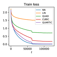
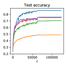
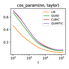
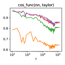
Figure 4: $k$-th order Taylorized training approximates full training increasingly better with $k$ on the CNNTHICK model. Training statistics are plotted for { full, linearized, quadratic, cubic, quartic} models. Left to right: (1) training loss; (2) test accuracy; (3) cosine similarity between Taylorized and full training in the parameter space; (4) cosine similarity between Taylorized and full training in the function (logit) space. All models are trained on CIFAR-10 for 124000 steps, and a 10x learning rate decay happened at step {62000, 93000}.

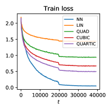
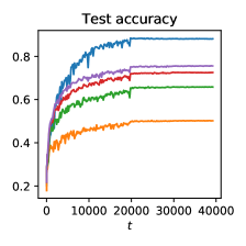
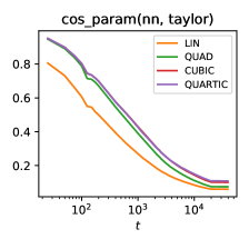
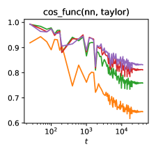
Figure 5: $k$-th order Taylorized training approximates full training increasingly better with $k$ on the WRNTHIN model. Training statistics are plotted for { full, linearized, quadratic, cubic, quartic} models. Left to right: (1) training loss; (2) test accuracy; (3) cosine similarity between Taylorized and full training in the parameter space; (4) cosine similarity between Taylorized and full training in the function (logit) space. All models are trained on CIFAR-10 for 39200 steps, and a 10x learning rate decay happened at step {19600, 29400}.

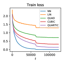
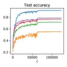
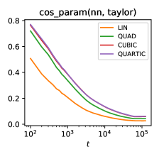
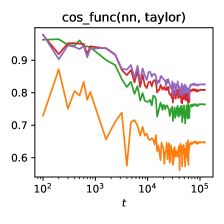
Figure 6: $k$-th order Taylorized training approximates full training increasingly better with $k$ on the WRNTHICK model. Training statistics are plotted for { full, linearized, quadratic, cubic, quartic} models. Left to right: (1) training loss; (2) test accuracy; (3) cosine similarity between Taylorized and full training in the parameter space; (4) cosine similarity between Taylorized and full training in the function (logit) space. All models are trained on CIFAR-10 for 124000 steps, and a 10x learning rate decay happened at step {62000, 93000}.

B.2 Effect of architectures / hyperparameters on Taylorized training

In this section, we study the effect of various architectural / hyperparameter choices on the approximation power of Taylorized training. We observe the following for $k$-th order Taylorized training for all $k\in{\left\{1,2,3,4\right\}}$:

• The approximation power gets slightly better (most significant in terms of the function-space similarity) when we increase the width (Section B.2.1).

• The approximation power gets significantly better when we use a smaller learning rate switch from the standard parameterization to the NTK parameterization. However, under both settings, the learning slows down dramatically and do not give a reasonably-performing model in 100 epochs (Section B.2.2).

We emphasize that (1) our observations largely agree with existing observations about linearized training (Lee et al., 2019), and (2) the point of these experiments is not to demonstrate the superiority of training settings such as small learning rate / NTK parameterization, but rather to show the advantage of considering Taylorized training with a higher $k$ (instead of linearized training) in practical training regimes that do not typically use a small learning rate or NTK parameterization.

B.2.1 Effect of width

We first examine the effect of width on the approximation power of Taylorized training. For this purpose, we compare Taylorized training on the {CNNTHIN, CNNTHICK} models; the CNNTHICK model has the same base architecture but is 4x wider then the CNNTHIN model. We train all models under identical optimization setups (note this different from our setting in the main paper). Results are reported in Table 3.

Observe that widening the network has no significant effect on the test performance gap and the parameter-space cosine similarity, but increases the function-space cosine similarity for all Taylorized models.

		test accuracy		cos_param(nn, taylor)		cos_func(nn, taylor)
		10 epochs	80 epochs	10 epochs	80 epochs	10 epochs	80 epochs
CNNTHIN (4 layers, 128 channels)	LIN ($k=1$)	36.67%	45.49%	0.079	0.031	0.626	0.618
	QUAD ($k=2$)	53.33%	64.55%	0.125	0.058	0.843	0.782
	CUBIC ($k=3$)	59.53%	70.50%	0.150	0.078	0.894	0.823
	QUARTIC ($k=4$)	61.96%	71.16%	0.150	0.079	0.904	0.828
	FULL NN	63.19%	78.98%	1.	1.	1.	1.
CNNTHICK (4 layers, 512 channels)	LIN ($k=1$)	38.88%	48.59%	0.081	0.037	0.671	0.648
	QUAD ($k=2$)	55.33%	67.60%	0.130	0.064	0.861	0.791
	CUBIC ($k=3$)	61.72%	71.86%	0.143	0.075	0.911	0.834
	QUARTIC ($k=4$)	63.67%	73.99%	0.150	0.076	0.921	0.841
	FULL NN	65.00%	85.09%	1.	1.	1.	1.

Table 3: Effect of width on Taylorized training. The two architectures are trained with the identical setting of batchsize=64, constant learning rate=$0.1$, and for 80 epochs. The cosine similarities are defined in Section 5.2. With a widened network, the function-space cosine similarity between neural net and Taylorized training becomes higher.

B.2.2 Effect of learning rate and NTK parameterization

In our second set of experiments, we study the effect of learning rate and/or network parameterization. We choose a base setting of the CNNTHIN architecture with standard parameterization and constant learning rate 0.1, and tweak it by (1) lowering the learning rate to 0.01, or (2) switching to the NTK parameterization. Results are reported in Table 4.

Observe that either lowering the learning rate or switching to NTK parameterization can dramatically improve the approximation power of Taylorized training (in terms of both function-space and parameter-space similarity), as well as the performance gap. However, either setting significantly slows down training (as indicated by the test performance of the full neural net).

		test accuracy		cos_param(nn, taylor		cos_func(nn, taylor)
		10 epochs	100 epochs	10 epochs	100 epochs	10 epochs	100 epochs
CNNTHIN standard param, lr$=0.1$	LIN ($k=1$)	32.94%	41.22%	0.156	0.049	0.649	0.605
	QUAD ($k=2$)	44.47%	59.90%	0.241	0.083	0.907	0.803
	CUBIC ($k=3$)	49.47%	67.07%	0.271	0.103	0.922	0.856
	QUARTIC ($k=4$)	52.13%	68.64%	0.272	0.115	0.920	0.867
	FULL NN	48.85%	77.47%	1.	1.	1.	1.
CNNTHIN standard param, lr$=0.01$	LIN ($k=1$)	26.40%	33.26%	0.356	0.138	0.544	0.604
	QUAD ($k=2$)	32.64%	49.01%	0.560	0.217	0.846	0.853
	CUBIC ($k=3$)	33.44%	54.34%	0.606	0.257	0.956	0.914
	QUARTIC ($k=4$)	35.22%	57.41%	0.622	0.272	0.971	0.926
	FULL NN	35.66%	58.84%	1.	1.	1.	1.
CNNTHIN NTK param, lr=$0.1$	LIN ($k=1$)	22.77%	27.43%	0.832	0.495	0.999	0.919
	QUAD ($k=2$)	22.56%	31.77%	0.898	0.692	0.999	0.987
	CUBIC ($k=3$)	22.70%	33.23%	0.899	0.707	0.999	0.993
	QUARTIC ($k=4$)	22.71%	33.53%	0.899	0.708	0.999	0.992
	FULL NN	21.12%	32.58%	1.	1.	1.	1.

Table 4: Effect of learning rate and parameterization on Taylorized training. All models are trained with the identical settings of batchsize=256 and for 100 epochs. The cosine similarities are defined in Section 5.2. Observe that using a lower learning rate or the NTK parameterization can significantly imporve the approximation accuracy of Taylorized models, but meanwhile will slow down the vanilla neural network training.

References

- Allen-Zhu & Li (2019) Allen-Zhu, Z. and Li, Y. What can resnet learn efficiently, going beyond kernels? In Advances in Neural Information Processing Systems, pp. 9015–9025, 2019.
- Allen-Zhu et al. (2019a) Allen-Zhu, Z., Li, Y., and Liang, Y. Learning and generalization in overparameterized neural networks, going beyond two layers. In Advances in neural information processing systems, pp. 6155–6166, 2019a.
- Allen-Zhu et al. (2019b) Allen-Zhu, Z., Li, Y., and Song, Z. A convergence theory for deep learning via over-parameterization. In International Conference on Machine Learning, pp. 242–252, 2019b.
- Arora et al. (2019a) Arora, S., Du, S., Hu, W., Li, Z., and Wang, R. Fine-grained analysis of optimization and generalization for overparameterized two-layer neural networks. In International Conference on Machine Learning, pp. 322–332, 2019a.
- Arora et al. (2019b) Arora, S., Du, S. S., Hu, W., Li, Z., Salakhutdinov, R. R., and Wang, R. On exact computation with an infinitely wide neural net. In Advances in Neural Information Processing Systems, pp. 8139–8148, 2019b.
- Arora et al. (2019c) Arora, S., Du, S. S., Li, Z., Salakhutdinov, R., Wang, R., and Yu, D. Harnessing the power of infinitely wide deep nets on small-data tasks. arXiv preprint arXiv:1910.01663, 2019c.
- Bai & Lee (2020) Bai, Y. and Lee, J. D. Beyond linearization: On quadratic and higher-order approximation of wide neural networks. In International Conference on Learning Representations, 2020. URL https://openreview.net/forum?id=rkllGyBFPH.
- Bradbury et al. (2018) Bradbury, J., Frostig, R., Hawkins, P., Johnson, M. J., Leary, C., Maclaurin, D., and Wanderman-Milne, S. JAX: composable transformations of Python+NumPy programs, 2018. URL http://github.com/google/jax.
- Cao & Gu (2019) Cao, Y. and Gu, Q. Generalization bounds of stochastic gradient descent for wide and deep neural networks. In Advances in Neural Information Processing Systems, pp. 10835–10845, 2019.
- Chizat & Bach (2018) Chizat, L. and Bach, F. On the global convergence of gradient descent for over-parameterized models using optimal transport. In Advances in neural information processing systems, pp. 3036–3046, 2018.
- Chizat et al. (2019) Chizat, L., Oyallon, E., and Bach, F. On lazy training in differentiable programming. 2019.
- Daniely (2017) Daniely, A. Sgd learns the conjugate kernel class of the network. In Advances in Neural Information Processing Systems, pp. 2422–2430, 2017.
- Du et al. (2019) Du, S., Lee, J., Li, H., Wang, L., and Zhai, X. Gradient descent finds global minima of deep neural networks. In International Conference on Machine Learning, pp. 1675–1685, 2019.
- Du et al. (2018) Du, S. S., Zhai, X., Poczos, B., and Singh, A. Gradient descent provably optimizes over-parameterized neural networks. arXiv preprint arXiv:1810.02054, 2018.
- Ghorbani et al. (2019a) Ghorbani, B., Mei, S., Misiakiewicz, T., and Montanari, A. Limitations of lazy training of two-layers neural network. In Advances in Neural Information Processing Systems, pp. 9108–9118, 2019a.
- Ghorbani et al. (2019b) Ghorbani, B., Mei, S., Misiakiewicz, T., and Montanari, A. Linearized two-layers neural networks in high dimension. arXiv preprint arXiv:1904.12191, 2019b.
- Glorot & Bengio (2010) Glorot, X. and Bengio, Y. Understanding the difficulty of training deep feedforward neural networks. In Proceedings of the thirteenth international conference on artificial intelligence and statistics, pp. 249–256, 2010.
- He et al. (2015) He, K., Zhang, X., Ren, S., and Sun, J. Delving deep into rectifiers: Surpassing human-level performance on imagenet classification. In Proceedings of the IEEE international conference on computer vision, pp. 1026–1034, 2015.
- Hu et al. (2020) Hu, W., Li, Z., and Yu, D. Simple and effective regularization methods for training on noisily labeled data with generalization guarantee. In International Conference on Learning Representations, 2020. URL https://openreview.net/forum?id=Hke3gyHYwH.
- Jacot et al. (2018) Jacot, A., Gabriel, F., and Hongler, C. Neural tangent kernel: Convergence and generalization in neural networks. In Advances in neural information processing systems, pp. 8571–8580, 2018.
- LeCun et al. (2015) LeCun, Y., Bengio, Y., and Hinton, G. Deep learning. nature, 521(7553):436–444, 2015.
- Lee et al. (2018) Lee, J., Sohl-dickstein, J., Pennington, J., Novak, R., Schoenholz, S., and Bahri, Y. Deep neural networks as gaussian processes. In International Conference on Learning Representations, 2018. URL https://openreview.net/forum?id=B1EA-M-0Z.
- Lee et al. (2019) Lee, J., Xiao, L., Schoenholz, S., Bahri, Y., Novak, R., Sohl-Dickstein, J., and Pennington, J. Wide neural networks of any depth evolve as linear models under gradient descent. In Advances in neural information processing systems, pp. 8570–8581, 2019.
- Li & Liang (2018) Li, Y. and Liang, Y. Learning overparameterized neural networks via stochastic gradient descent on structured data. In Advances in Neural Information Processing Systems, pp. 8157–8166, 2018.
- Li et al. (2019a) Li, Y., Wei, C., and Ma, T. Towards explaining the regularization effect of initial large learning rate in training neural networks. In Advances in Neural Information Processing Systems, pp. 11669–11680, 2019a.
- Li et al. (2019b) Li, Z., Wang, R., Yu, D., Du, S. S., Hu, W., Salakhutdinov, R., and Arora, S. Enhanced convolutional neural tangent kernels. arXiv preprint arXiv:1911.00809, 2019b.
- Matthews et al. (2018) Matthews, A. G. d. G., Rowland, M., Hron, J., Turner, R. E., and Ghahramani, Z. Gaussian process behaviour in wide deep neural networks. arXiv preprint arXiv:1804.11271, 2018.
- Mei et al. (2018) Mei, S., Montanari, A., and Nguyen, P. A mean field view of the landscape of two-layers neural networks. Proceedings of the National Academy of Sciences, 115:E7665–E7671, 2018.
- Mondelli & Montanari (2019) Mondelli, M. and Montanari, A. On the connection between learning two-layer neural networks and tensor decomposition. In The 22nd International Conference on Artificial Intelligence and Statistics, pp. 1051–1060, 2019.
- Mu et al. (2020) Mu, F., Liang, Y., and Li, Y. Gradients as features for deep representation learning. In International Conference on Learning Representations, 2020. URL https://openreview.net/forum?id=BkeoaeHKDS.
- Neal (1996) Neal, R. M. Priors for infinite networks. In Bayesian Learning for Neural Networks, pp. 29–53. Springer, 1996.
- Novak et al. (2020) Novak, R., Xiao, L., Hron, J., Lee, J., Alemi, A. A., Sohl-Dickstein, J., and Schoenholz, S. S. Neural tangents: Fast and easy infinite neural networks in python. In International Conference on Learning Representations, 2020. URL https://openreview.net/forum?id=SklD9yrFPS.
- Pearlmutter (1994) Pearlmutter, B. A. Fast exact multiplication by the hessian. Neural computation, 6(1):147–160, 1994.
- Rotskoff & Vanden-Eijnden (2018) Rotskoff, G. M. and Vanden-Eijnden, E. Neural networks as interacting particle systems: Asymptotic convexity of the loss landscape and universal scaling of the approximation error. arXiv preprint arXiv:1805.00915, 2018.
- Sirignano & Spiliopoulos (2018) Sirignano, J. and Spiliopoulos, K. Mean field analysis of neural networks. arXiv preprint arXiv:1805.01053, 2018.
- Wei et al. (2019) Wei, C., Lee, J. D., Liu, Q., and Ma, T. Regularization matters: Generalization and optimization of neural nets vs their induced kernel. In Advances in Neural Information Processing Systems, pp. 9709–9721, 2019.
- Yang (2019) Yang, G. Tensor programs i: Wide feedforward or recurrent neural networks of any architecture are gaussian processes. arXiv preprint arXiv:1910.12478, 2019.
- Yehudai & Shamir (2019) Yehudai, G. and Shamir, O. On the power and limitations of random features for understanding neural networks. In Advances in Neural Information Processing Systems, pp. 6594–6604, 2019.
- Zagoruyko & Komodakis (2016) Zagoruyko, S. and Komodakis, N. Wide residual networks. arXiv preprint arXiv:1605.07146, 2016.
- Zhang et al. (2019) Zhang, C., Bengio, S., and Singer, Y. Are all layers created equal? arXiv preprint arXiv:1902.01996, 2019.
- Zou et al. (2019) Zou, D., Cao, Y., Zhou, D., and Gu, Q. Gradient descent optimizes over-parameterized deep relu networks. Machine Learning, pp. 1–26, 2019.