Quantitative Coding and Complexity Theory
of Continuous Data

Abstract

Specifying a computational problem includes fixing encodings for input and output: encoding graphs as adjacency matrices, characters as integers, integers as bit strings, and vice versa. For such discrete data, the actual encoding is usually straightforward and/or complexity-theoretically inessential (up to linear or polynomial time, say). Concerning continuous data, already real numbers naturally suggest various encodings (formalized as historically so-called representations) with very different properties, ranging from the computably ‘unreasonable’ binary expansion [doi:10.1112/plms/s2-43.6.544] via qualitatively to polynomially and even linearly complexity-theoretically ‘reasonable’ signed-digit expansion. But how to distinguish between un/suitable encodings of other spaces common in Calculus and Numerics, such as Sobolev?

With respect to qualitative computability over topological spaces, admissibility had been identified [doi:10.1016/0304-3975(85)90208-7] as a crucial criterion for a representation over the Cantor space of infinite binary sequences to be ‘reasonable’: It requires the representation to be (sequentially) continuous, and to be maximal with respect to (sequentially) continuous reduction [doi:10.1007/11780342_48]. Such representations are guaranteed to exist for a large class of spaces. And for (precisely) these does the sometimes so-called Main Theorem hold: which characterizes continuity of functions by the continuity of mappings translating codes, so-called realizers.

We refine qualitative computability over topological spaces to quantitative complexity over metric spaces, by developing the theory of polynomially and of linearly admissible representations. Informally speaking, these are ‘optimally’ continuous, namely linearly/polynomially relative to the space’s entropy; and maximal with respect to relative linearly/polynomially continuous reductions defined below. A large class of spaces is shown to admit a quantitatively admissible representation, including a generalization of the signed-digit encoding; and these exhibit a quantitative strengthening of the qualitative Main Theorem, namely now characterizing quantitative continuity of functions by quantitative continuity of realizers. Our quantitative admissibility thus provides the desired criterion for complexity-theoretically ‘reasonable’ encodings.

We then rephrase quantitative admissibility as quantitative continuity of both the representation and of its set-valued inverse, the latter adopting from [doi:10.4115/jla.2013.5.7] a new notion of ‘sequential’ continuity for multifunctions. By establishing a quantitative continuous selection theorem for multifunctions between compact ultrametric spaces, we can extend our above quantitative Main Theorem from functions to multifunctions aka search problems. Higher-type complexity is captured by generalizing Cantor’s (and Baire’s) ground space for encodings to other (compact) ultrametric spaces.

1 Introduction

Machine models formalize computation: Such a model specifies the ways to input, operate on, and output elements from some fixed ‘ground’ space $\mathcal{U}$; as well as a measure of cost, and of parameter(s) in whose dependence to analyze and bound said computational cost. Computational problems over spaces $X$ other than $\mathcal{U}$ are treated by encoding its elements/instances over $\mathcal{U}$, formalized as representations: surjective partial mappings $\xi:\subseteq\mathcal{U}\twoheadrightarrow X$.

Machine models formalize computation: Such a model specifies the ways to input, operate on, and output elements from some fixed ‘ground’ space $\mathcal{U}$; as well as a measure of cost, and of parameter(s) in whose dependence to analyze and bound said computational cost. Computational problems over spaces $X$ other than $\mathcal{U}$ are treated by encoding its elements/instances over $\mathcal{U}$, formalized as representations: surjective partial mappings $\xi:\subseteq\mathcal{U}\twoheadrightarrow X$.

Example 1

1. Recall the Turing machine model operating on the set $\mathcal{U}=\{\textup{{0}},\textup{{1}}\}^{*}$ of finite binary sequences. Operations amount to local transformations of (and in local dependence on) the tape contents. And computational cost is measured in dependence on the binary length $n\in\mathbb{N}$ of the input $\vec{x}\in\{\textup{{0}},\textup{{1}}\}^{n}$.

2. Computing over the countable space $X$ of finite graphs proceeds by encoding them over $\{\textup{{0}},\textup{{1}}\}^{*}$: for example as adjacency matrices’ binary entries. Cost parameter $n\in\mathbb{N}$ commonly denotes the number of nodes of the graph, or the binary length of the encoded matrix: both are polynomially related to each other.

3. Consider the countable space $X=\mathbb{N}$ of natural numbers. Turing-computation encodes $\mathbb{N}$ also over $\{\textup{{0}},\textup{{1}}\}^{*}$ from (a), for instance in binary or in unary: These are computably related, and therefore induce the same notions of computability on $\mathbb{N}$; but their lengths, and induced notions of complexity, are not polynomially related.

4. Recall the type-2 machine model [Wei00, §2.1] operating on the Cantor space $\mathcal{C}:=\{\textup{{0}},\textup{{1}}\}^{\mathbb{N}}$ of infinite binary sequences equipped with the metric $D:(\bar{u},\bar{v})\;\mapsto\;2^{-\min\{n:u_{n}\neq v_{n}\}}$. The computation of such a machine amounts to a partial transformation $F:\bar{u}\mapsto\bar{v}=(v_{n})$ from/to $\mathcal{C}$. Equivalently via currying, the machine on input of ‘infinite’ $\bar{u}\in\mathcal{C}$ and of ‘finite’ $\textup{{1}}^{n}$ (encoding $n\in\mathbb{N}$ in unary) prints $v_{n}$: the $n$-th entry of the output sequence $\bar{v}\in\mathcal{C}$.
   Computational cost is commonly gauged in dependence of the index position $n$ within the binary output sequence, that is, the length of the finite initial segment $\bar{v}_{<n}=(v_{0},v_{1},\ldots,v_{n-1})$ written so far [Wei00, §7.1]; equivalently: the length $n$ of the finite part $\textup{{1}}^{n}$ of the input. In either case, a computational cost bound $t=t(n)$ must not depend on the infinite part $\bar{u}$ of the input. It follows that any partial $F:\subseteq\mathcal{C}\to\mathcal{C}$ computed in time $t:\mathbb{N}\to\mathbb{N}$ has modulus of continuity $t$ according to Subsection 1.2.

5. Computation on the real unit interval $X=[0;1]$ proceeds by encoding $X$ over ground space $\mathcal{C}$, in various ways:

6. The binary expansion renders tripling $[0;1/3]\ni r\mapsto 3r\in[0;1]$ uncomputable and is therefore unsuitable [Tur38, p.546]. To see this, start with $1/6=(\textup{{0}}.\textup{{0}}\textup{{0}}\textup{{1}}\textup{{0}}\textup{{1}}\textup{{0}}\textup{{1}}\ldots)_{2}$ and consider, arbitrarily far off in the expansion, either replacing some single digit 0 with 1 or replacing some single digit 1 with 0: The result of tripling in the first case will begin with $(\textup{{0}}.\textup{{1}}\ldots)_{2}$ yet in the second case begin with $(\textup{{0}}.\textup{{0}}\ldots)_{2}$. To algorithmically output the first binary digit after the binary point thus would require ‘knowing’ all infinitely many binary digits of the input: contradiction [Wei00, Exercise 7.2.7].

7. Let $r\in[0;1]$ be encoded as any sequence

   $$\big{(}\mathrm{bin}(a_{0}),\mathrm{bin}(c_{0}),\ldots,\mathrm{bin}(a_{n}),\mathrm{bin}(c_{n}),\ldots\big{)}\;\in\;\mathcal{C}$$ (1)

   of binary numerators and denominators $a_{n},c_{n}\in\mathbb{N}$ of rational approximations satisfying $|r-a_{n}/c_{n}|\leq 1/2^{n}$. This representation induces the ‘standard’ notion of real computability [Grz57]. In particular every (qualitatively) computable partial real function must be (qualitatively) continuous [Wei00, Theorem 4.3.1]. But this representation induces no reasonable notion of computational complexity.
   To see this, consider the number $t\in\mathbb{N}$ of steps some algorithm makes; and these steps include skipping some number $\mu(n)\leq t(n)$ of bits in the infinite string from Equation (1) in order to reach and extract $a_{n}/c_{n}$ as guaranteed approximation to $r$ up to $1/2^{n}$. For $r:=1/2$ with $a_{n}:=1+2^{k_{n}}$ and $c_{n}:=2^{1+k_{n}}$ with sufficiently large integers $k_{n}\geq n$, this number $\mu(n)$ can be arbitrarily large, meaning that the running time $t\geq\mu$ of such an algorithm cannot be bounded in terms of the precision parameter $n$ [Wei00, Examples 7.2.1+7.2.3]. Note that, compared to the required approximation error bound $1/2^{n}$, denominators $2^{k_{n}}$ in this counterexample are exceedingly large—which Item (e iii) prevents.

Here and in the sequel, $\mathrm{bin}:\mathbb{N}\to\{\textup{{0}},\textup{{1}}\}^{*}$ denotes binary expansion of natural numbers with delimiter quelling leading 0s:

$$\mathrm{bin}:\mathbb{N}\to\{\textup{{0}},\textup{{1}}\}^{*},\quad 0\;\mapsto\;\textup{{0}}\,\textup{{1}},\\ \{2^{n},\ldots,2^{n+1}-1\}\;\ni\;2^{n}+2^{n-1}b_{n-1}+2^{n-2}b_{n-2}+\cdots+2b_{1}+b_{0}\;\mapsto\;\\ \mapsto\;(\textup{{1}}\,\textup{{0}}\,b_{n-1}\,\textup{{0}}\,\ldots b_{1}\,\textup{{0}}\,b_{0}\,\textup{{1}})\;\in\;\{\textup{{0}},\textup{{1}}\}^{2n+2}\enspace.$$

1. Consider encoding $r\in[0;1]$ over $\mathcal{C}$ as sequence $\big{(}\mathrm{bin}(a_{1}),\ldots,\mathrm{bin}(a_{n}),\ldots\big{)}$ of numerators $a_{n}\in\mathbb{N}$ of dyadic approximations satisfying $|r-a_{n}/2^{n}|\leq 1/2^{n}$. This induces the same notion of real computability as (e ii). And, again, computational cost counts the number $t(n)$ of steps until output of (the numerator $a_{n}$ to) an approximation up to absolute error $1/2^{n}$; or until output of the $n$-th bit of $\big{(}\mathrm{bin}(a_{1}),\ldots,\mathrm{bin}(a_{m}),\ldots\big{)}\in\mathcal{C}$: Both parameters are polynomially related to each other: $\big{(}\mathrm{bin}(a_{1}),\ldots,\mathrm{bin}(a_{n})\big{)}$ has binary length between $n$ and $\mathcal{O}(n^{2})$, and in particular is bounded polynomially in $n$. This renders arithmetic (addition, subtraction, multiplication, division) of real numbers computable in polynomial time. Moreover any partial real function computed in time $t:\mathbb{N}\to\mathbb{N}$ has modulus of continuity $\operatorname{poly}\Big{(}t\big{(}\operatorname{poly}(n)\big{)}\Big{)}$; cmp. Corollary 1 below.

2. Encode $x\in[0;1]$ as signed binary expansion $x=1/2+\sum_{m\geq 0}s_{m}\cdot 2^{-m-2}$ with $s_{n}\in\{-1,0,1\}\cong\{\textup{{0}}\textup{{0}},\textup{{0}}\textup{{1}},\textup{{1}}\textup{{0}}\}$. Again, computational cost counts the number of steps until output of approximation $1/2+\sum_{m\leq n}s_{m}\cdot 2^{-m-2}$ up to absolute error $1/2^{n}$; or until output of the $n$-th (signed) output bit of $(s_{0},\ldots,s_{n},\ldots\big{)}$: Both are linearly related to each other. They render addition of real numbers computable by a finite transducer (see Figure 3 below) and in particular in linear time [Wei00, Theorem 7.3.1]. Note that $[0;1]^{2}\ni(x,y)\mapsto x+y\in[0;2]$ has modulus of continuity $\mu(n)=n+\mathcal{O}(1)$. Conversely, any partial real function computed in time $t$ has a modulus of continuity $\mathcal{O}\Big{(}t\big{(}\mathcal{O}(n)\big{)}\Big{)}$; cmp. Corollary 1 below.

3. Recall the oracle Turing machine model, allowed to query some oracle $\varphi\subseteq\{\textup{{0}},\textup{{1}}\}^{*}$. Equivalently via currying: query a total string predicate $\varphi:\{\textup{{0}},\textup{{1}}\}^{*}\to\{\textup{{0}},\textup{{1}}\}$. Considering the oracle as variable [KC12, §3] leads to computation as a transformation $\Lambda:\varphi\mapsto\psi$ from/to the space $\mathcal{B}=(\{\textup{{0}},\textup{{1}}\}^{*})^{\dagger}$ of total string predicates; equivalently via currying: $\Lambda:(\{\textup{{0}},\textup{{1}}\}^{*})^{\dagger}\times\{\textup{{0}},\textup{{1}}\}^{*}\ni(\varphi,\vec{x})\mapsto\psi(\vec{x})\in\{\textup{{0}},\textup{{1}}\}$.
   Cost here is to be bounded in dependence of the binary input length $n=|\vec{x}|$ of the finite part of the input, but independently of the infinite part $\varphi\in\operatorname{dom}(\Lambda)$. Equipping $(\{\textup{{0}},\textup{{1}}\}^{*})^{\dagger}$ with the metric $D:(\varphi,\psi)\mapsto 2^{-\min\{|\vec{x}|:\varphi(\vec{x})\neq\psi(\vec{x})\}}$, any partial $\Lambda:\subseteq(\{\textup{{0}},\textup{{1}}\}^{*})^{\dagger}\to(\{\textup{{0}},\textup{{1}}\}^{*})^{\dagger}$ computable in time $t$ has modulus of continuity $t$.

4. Spaces $X$ of continuum cardinality beyond real numbers (e) are also commonly encoded over Cantor space $\mathcal{C}=\{\textup{{0}},\textup{{1}}\}^{\mathbb{N}}$ [Wei00, §3], or over oracle space $\mathcal{B}=(\{\textup{{0}},\textup{{1}}\}^{*})^{\dagger}$ [KC12, §3.4]; see [ZZ99, Zie03, Sch07] for some examples.
   Computability-theoretically ‘reasonable’ representations are the admissible ones [Wei00, Theorem 3.2.9.2]; cmp. [KW85, Sch02]: (Precisely) these make continuous functions correspond to continuous translations on Cantor/oracle space and vice versa [Wei00, Theorem 3.2.11]. The encodings of real numbers from Items (e ii) to (e iv) are admissible, but the binary one in (e i) is not.

5. Search problems admit possibly more than one answer/output to a given input. For example the Fundamental Theorem of Algebra assigns to any $d$-tuple of complex coefficients $(c_{0},\ldots,c_{d-1})\in\mathbb{C}^{d}$ some $d$-tuple $(z_{1},\ldots,z_{d})\in\mathbb{C}^{d}$ of complex roots (including multiplicity) of the polynomial $c_{0}+c_{1}Z+\cdots+c_{d-1}Z^{d-1}+Z^{d}$. This non-uniqueness of the answer is modeled by a (set-valued aka) multi-function $\mathbb{C}^{d}\rightrightarrows\mathbb{C}^{d}$, $(c_{0},\ldots,c_{d-1})\Mapsto(z_{1},\ldots,z_{d})$; cmp. [Luc77].

To summarize, common models of computation (Turing machine, type-2 machine, oracle machine) naturally operate on certain ‘basic’ spaces (finite binary strings $\{\textup{{0}},\textup{{1}}\}^{*}$, Cantor space $\mathcal{C}=\{\textup{{0}},\textup{{1}}\}^{\mathbb{N}}$, oracle space $(\{\textup{{0}},\textup{{1}}\}^{*})^{\dagger}$) with computational cost bounded in dependence of the binary length $n$ of the finite part of inputs, but independently of the infinite parts. Computation on other spaces proceeds by encoding them over such basic spaces; and computing a function between such spaces amounts to translating codes of arguments to codes of values.

Note that, for computability questions, equilogical spaces have been suggested as basic spaces [BBS04]. Regarding complexity questions, we suggest to generalize $\mathcal{C}$ and $(\{\textup{{0}},\textup{{1}}\}^{*})^{\dagger}$, namely to consider compact ultrametric spaces of diameter 1 as basic spaces over which to encode other spaces. This choice will be justified in Subsection 3.3. Recall that an ultrametric $D$ satisfies the following strong triangle inequality:

$$D(x,z)\;\leq\;\max\big{\{}\>D(x,y)\>,\>D(y,z)\;\}\enspace.$$ (2)

The present work addresses the following question:

Question 1

Fix some compact metric space $X$ and a compact ultrametric ground space $\mathcal{U}$. Which encodings of $X$ over $\mathcal{U}$ are ‘suitable’ with respect to computational complexity?

Recall (Example 1g) that, for computability (rather than complexity) purposes, admissibility has been established as answer to this Question 1.

1.1 Previous/Related Work and Overview

Computability, and qualitative coding theory, for continuous data dates back at least to Turing for the real case [Tur37]; and to Kreitz and Weihrauch for the case of second-countable T0 spaces [KW85], see Fact 1.1 below and the standard textbook [Wei00]; with generalization to further spaces mostly due to Schröder [Sch01, Sch02, Sch06].

Early rigorous bit-complexity investigations, and quantitative coding considerations over the reals [KF82, Fri84, Mül86, DK89], had culminated in the textbook [Ko91]; see [Kaw10, KC12, KO14] for recent work—and [Wei03, KMRZ15, SS17, Ste17] for first algorithmic cost and coding considerations of spaces beyond continuous real functions.

The bit-complexity questions pursued there and in the present work are not to be confused with Information-Based/Algebraic Complexity Theory based on the unit-cost aka Blum-Shub-Smale aka real-RAM model [JHG88, BCSS98, PB97, dBvKOC08]. The latter model also underlies the Nyquist-Shannon Sampling Theorem, revolving around encoding certain real functions by the least number of real numbers—each one still an infinite object: The present work is closer to Approximation and Information Theory [HHW55].

Embedding finite/countable metric spaces into trees (as particular cases of ultrametric spaces) with least distortion is a well-studied problem [IM04]; and the present work considers encoding uncountably infinite spaces over the infinite tree of Cantor space.

Subsection 1.2 collects some mathematical basics of metric spaces, with emphasis on quantitative properties like entropy and modulus of continuity. Subsection 1.3 recalls the Kreitz-Weihrauch framework of encoding continuous data over Cantor space. Their qualitative key property, admissibility, yields the Main Theorem (Fact 1.1). Four ways of encoding the real unit interval illustrate important differences regarding computability and complexity. They serve as guide in Section 2 to our new quantitative version of admissibility (Definition 2); and yield the new, quantitative Main Theorem 2.1 in Subsection 2.1, proven in Subsection 2.4. Theorem 2.3 asserts a large class of compact metric spaces to admit quantitatively admissible representations over Cantor space, including a generalization of the signed binary representation.

qualitative	computability	topology	(uniform) continuity	compactness	equilogical
quantitative	complexity	metric	modulus of continuity	entropy	ultrametric

Table 1: “Dictionary” between qualitative and quantitative coding of continuous data.

Section 3 takes an alternative approach to quantitatively refine qualitative admissibility: from the perspective of a logical (as opposed to topological) notion of continuity for multifunctions from [BH94, PZ13]. To this end Subsection 3.1 recalls some terminology concerning multifunctions. Then Subsection 3.2 motivates and introduces a quantitative version of continuity for multifunctions. Our quantitative selection theorem for multifunctions between compact ultrametric spaces in Subsection 3.3 applies and builds on this notion. It leads in Subsection 3.5 to a quantitative Main Theorem 3.4 for multifunctions between spaces equipped with quantitatively admissible representations over suitable generalized (namely quantitatively homogeneous and quantitatively admissible) domains.

1.2 Recap of Metric Spaces

Like resource-bounded complexity quantitatively refines qualitative computability, this subsection recalls relevant metric properties that quantitatively refine qualitative topological properties of the mathematical spaces under consideration.

Following [Wei03, §6], a (binary) modulus of continuity of a function $f:X\to Y$ between metric spaces $(X,d)$ and $(Y,e)$ is a non-decreasing mapping $\mu:\mathbb{N}\to\mathbb{N}$ such that

$$d(x,x^{\prime})\;\leq\;2^{-\mu(n)}\quad\Rightarrow\quad e\big{(}f(x),f(x^{\prime})\big{)}\;\leq\;2^{-n}\enspace.$$ (3)

Equivalently: the induced semi-metric

$$e_{f}:f[X]\times f[X]\;\ni\;(y,y^{\prime})\;\mapsto\;\min\big{\{}d(x,x^{\prime})\>:\>f(x)=y,f(x^{\prime})=y^{\prime}\big{\}}$$ (4)

satisfies $e_{f}(y,y^{\prime})\leq 2^{-\mu(n)}\Rightarrow e(y,y^{\prime})\leq 2^{-n}$. Note that $e_{f}$ is well-defined whenever $f$ is continuous with compact domain, but may violate the triangle inequality. Call a modulus of continuity $\mu$ of $f$ minimal if it is pointwise minimal among those satisfying Equation (3) and/or (4).

Remark 1

The integer $m=\mu(n)$ roughly captures the number of bits of approximations to arguments $x$ sufficient to guarantee $n$ bits of approximation to $y=f(x)$.

1. Precisely the uniformly continuous functions have a (minimal) modulus of continuity.

2. Suppose $X$ is compact or convex complete or $Y$ is bounded. Then Lipschitz-continuous functions $f:X\to Y$ are precisely those with modulus $\mu(n)=n+\mathcal{O}(1)$. And Hölder-continuous functions $f:X\to Y$ are precisely those with linear modulus $\mu(n)=\mathcal{O}(n)$.

3. If $f:X\to Y$ has modulus of continuity $\mu$ and $g:Y\to Z$ has modulus of continuity $\nu$, the $g\circ f$ has modulus of continuity $\mu\circ\nu$.

4. The function $h:(0;1]\ni t\mapsto 1/\ln(e/t)\in(0;1]$ from Figure 1 extends uniquely continuously to $0$. It has an exponential, but no polynomial, modulus of continuity.

5. The $k$-fold iterate of $h:[0;1]\to[0;1]$ from (d) has modulus of continuity an exponential tower of height $k$, but not of height $k-1$.

For self-containment, a proof is provided at the end of this subsection. Recall that a (not necessarily linear) metric space $(X,d)$ is convex if, to any $x,z\in X$ there exists $y\in X$ distinct from $x,z$ with $d(x,z)=d(x,y)+d(y,z)$.

Figure 1:

Abbreviate with $\overline{\operatorname{B}}(x,r)=\{x^{\prime}:d(x,x^{\prime})\leq r\}\subseteq X$ the closed ball with center $x\in X$ and radius $r>0$, and let $\operatorname{diam}(X)=\sup\{d(x,y):x,y\in Y\}$ denote the diameter of $X$. The present work considers representations over compact ultrametric spaces of diameter 1, a rich class of spaces:

Lemma 1

1. Any finite set, when equipped with the discrete metric, constitutes a compact ultrametric space of diameter 1.
   

2. Equip the space $\{\textup{{0}},\textup{{1}}\}^{*}$ of finite binary strings with the ultrametric

   $$D(\vec{u},\vec{v})\;:=\;2^{-\min\{n\>:\>n\geq|\vec{u}|\>\vee\>n\>\geq\>|\vec{v}|\>\vee\>u_{n}\neq v_{n}\}}\enspace:$$

   Its completion $\{\textup{{0}},\textup{{1}}\}^{*}\uplus\mathcal{C}$ is compact with diameter 1. Same for the space $\{\textup{{0}},\textup{{1}}\}^{+}$ of non-empty finite binary strings with ultrametric $2D$.

3. Let $(U,D)$ and $(V,E)$ denote compact (ultra)metric spaces of diameter 1. The Cartesian product $U\times V$ is again an (ultra)metric space of diameter 1 when equipped with the maximum metric

   $$D\times E\;:=\;\max\{D,E\}\;:\;\big{(}(u,v),(u^{\prime},v^{\prime})\big{)}\;\mapsto\;\max\big{\{}D(u,u^{\prime}),E(v,v^{\prime})\big{\}}\enspace.$$ (5)

   Similarly/inductively for the Cartesian product of finitely many (ultra)metric spaces of diameter 1.

4. Let $(U,D)$ denote a compact metric space and $(V,E)$ a compact (ultra)metric space of diameter 1. Consider the space $\operatorname{Lip}_{1}(U,V)$ of total functions $f:U\to V$ which are non-expansive (aka 1-Lipschitz) in satisfying

   $$\forall u,u^{\prime}\in U:\quad E\big{(}f(u),f(u^{\prime})\big{)}\;\leq\;D(u,u^{\prime})\enspace.$$ (6)

   Equipped with the supremum metric $E^{U}(f,g)=\sup\big{\{}e\big{(}f(u),g(u)\big{)}:u\in U\big{\}}$, $\operatorname{Lip}_{1}(U,V)$ is again a compact (ultra)metric space of diameter 1.

5. Fix compact (ultra)metric spaces $(U_{j},D_{j})$ of diameter 1, $j\in J\subseteq\mathbb{N}$. Their Cartesian product $\prod_{j\in J}U_{j}$ is again compact of diameter $\leq 1$ when equipped with the (ultra)metric

   $$\prod\nolimits_{j\in J}D_{j}/2^{j}\>:\>\big{(}(u_{j})_{{}_{j}},(u^{\prime}_{j})_{{}_{j}}\big{)}\;\mapsto\;\max\big{\{}D_{j}(u_{j},u^{\prime}_{j})/2^{j}:j\in J\big{\}}\enspace.$$ (7)

Note that Cantor space $\mathcal{C}$ is recovered from Lemma 1e) with $U_{j}:\equiv\{\textup{{0}},\textup{{1}}\}$ according to (a). Also oracle space $(\{\textup{{0}},\textup{{1}}\}^{*})^{\dagger}$ arises from Lemma 1e), namely with the finite Cartesian products $U_{j}:=\prod_{\{\textup{{0}},\textup{{1}}\}^{j}}\{\textup{{0}},\textup{{1}}\}=\{\textup{{0}},\textup{{1}}\}^{\{\textup{{0}},\textup{{1}}\}^{j}}$, $j\geq 0$, equipped with the discrete metric according to (a). $\operatorname{Lip}_{1}(\mathcal{C},\mathcal{C})$ is a compact ultrametric space of diameter 1 according to Lemma 1d); and isometric to $(^{\dagger}\{\textup{{0}},\textup{{1}}\}^{+})=\prod_{j\geq 0}\{\textup{{0}},\textup{{1}}\}^{(\{\textup{{0}},\textup{{1}}\}^{j+1})}$ according to Lemma 1e). The following lemma generalizes this isometry:

Lemma 2

Let $U_{j},V_{j}$ denote sequences of finite sets, equipped with the discrete metric. Consider the compact ultrametric spaces $U=\prod_{j}U_{j}$ and $V=\prod_{j}V_{j}$ according to Lemma 1e). Then $\operatorname{Lip}_{1}(U,V)$ according to Lemma 1d) is isometric to $\prod_{j}W_{j}$ according to Lemma 1e), where

$$W_{j}\;:=\;\prod\nolimits_{U_{0}\times U_{1}\times\cdots\times U_{j}}V_{j}\;=\;V_{j}^{U_{0}\times U_{1}\times\cdots\times U_{j}}\enspace.$$

Recall [KT59] that the unary entropy of $X$, also known as its width [Wei03, §6], is the mapping $\widehat{\eta}=\widehat{\eta}_{X}:\mathbb{N}\to\mathbb{N}\cup\{\infty\}$ such that $X$ can by covered by $\widehat{\eta}(n)$, but not by less, closed balls $\overline{\operatorname{B}}(x,2^{-n})$ of radius $2^{-n}$ around centers $x\in X$. To match the binary conception of the modulus (3), we here focus on the binary entropy $\eta_{X}=\lceil\log_{2}\widehat{\eta}_{X}\rceil$, and call it just entropy [Wal82, KSZ16, Ste17]; cmp. Remark 2 below.

Lemma 3

The integer $m=\eta(n)$ roughly describes the number of bits sufficient and necessary to specify, for every possible $x\in X$, some approximation up to error $2^{-n}$.

1. Cantor space has entropy $\eta(n)=n$; the real unit interval $[0;1]$ has entropy $\eta(n)=\max\{n-1,0\}$. The Hilbert Cube $\mathcal{H}=\prod_{j\geq 0}[0;1]$ with metric ((7)) has quadratic entropy $\eta(n)=\Theta(n^{2})$.

2. Generalizing Example 1f), fix some non-empty $\Phi\subseteq\{\textup{{0}},\textup{{1}}\}^{*}$ and let $\Phi^{\dagger}:=\{\textup{{0}},\textup{{1}}\}^{\Phi}$ denote the collection of total string predicates $\varphi:\Phi\to\{\textup{{0}},\textup{{1}}\}$. Equip $\Phi^{\dagger}$ with the ultrametric $D(\varphi,\varphi^{\prime})=1/2^{\min{|\vec{v}|:\varphi(\vec{v})\neq\varphi(\vec{v}^{\prime})}}$. $\Phi^{\dagger}$ is compact with entropy $\eta_{\Phi^{\dagger}}(n)=\operatorname{Card}\Phi_{<n}$, where $\Phi_{<m}:=\Phi\cap\{\textup{{0}},\textup{{1}}\}^{<m}$ and $\{\textup{{0}},\textup{{1}}\}^{<m}=\bigcup_{n<m}\{\textup{{0}},\textup{{1}}\}^{n}$.

3. Let compact $(X,d)$ and $(Y,e)$ have entropies $\eta_{X}$ and $\eta_{Y}$, respectively. Then the entropy $\eta_{X\times Y}$ of compact $\big{(}X\times Y,\max\{d,e\}\big{)}$ satisfies

   $$\forall n>0:\quad\eta_{X}(n-1)+\eta_{Y}(n-1)\;\leq\;\eta_{X\times Y}(n)+1\;\leq\;\eta_{X}(n)+\eta_{Y}(n)+1\enspace.$$

4. Let compact $(X_{j},d_{j})$ have diameters $\leq 1$ and entropy $\eta_{j}$ for each $j\in\mathbb{N}$. Then $\big{(}\prod_{j}X_{j},\sup_{j}d_{j}/2^{j}\big{)}$ is compact and has entropy $\eta$ satisfying

   $$\forall n>0:\quad\sum\nolimits_{j<n}\eta_{j}(n-j-1)\;\leq\;1\>+\>\eta(n)\;\leq\;1\>+\>\sum\nolimits_{j\leq n}\eta_{j}(n-j)\enspace.$$

5. Fix a compact metric space $(X,d)$ with entropy $\eta$. Let $\mathcal{K}(X)$ denote the set of non-empty closed subsets of $X$ and equip it with the Hausdorff metric

   $$d_{\mathcal{K}}(V,W)\;\mapsto\;\max\big{\{}\sup\{d_{V}(w):w\in W\},\sup\{d_{W}(v):v\in V\}\big{\}},$$ (8)

   where $d_{V}:X\ni x\mapsto\inf\{d(x,v):v\in V\}\in\operatorname{Lip}_{1}(X,\mathbb{R})$ denotes $V$’s distance function. Then $\big{(}\mathcal{K}(X),d_{\mathcal{K}}\big{)}$ constitutes a compact metric space [Wei00, Exercise 8.1.10]. It has entropy $H\leq 2^{\eta}$ with $2^{\eta(n)-1}<H(n+1)$.

6. Fix a connected compact metric space $(X,d)$ with entropy $\eta$, and consider the convex metric space $X^{\dagger}:=\operatorname{Lip}_{1}(X,[0;1])$ of non-expansive (=1-Lipschitz) real functions equipped with the supremum norm $|f|=\sup_{x\in X}|f(x)|$, compact by Arzelá-Ascoli. This has entropy $\eta^{\dagger}(n):=\eta_{X^{\dagger}}(n)=\Theta\big{(}2^{\eta(n\pm\mathcal{O}(1))}\big{)}$; more precisely it holds: $2^{\eta(n-1)-1}\;<\;\eta^{\dagger}(n)\;\leq\;\mathcal{O}\big{(}2^{\eta(n+2)}\big{)}$; see Figure 2.

7. For $f:X\to Y$ a mapping between metric spaces with modulus of continuity $\mu$, the image $f[X]\subseteq Y$ has entropy $\eta_{f[X]}\leq\eta_{X}\circ\mu$; cmp. [Ste16, Lemma 3.1.13].

8. Every connected compact metric space $X$ has entropy at least linear $\eta(n)\geq n+\Omega(1)$.

9. Fix an arbitrary non-decreasing unbounded mapping $\nu:\mathbb{N}\to\mathbb{N}$ and re-consider Cantor space $\mathcal{C}$ but now equipped with $D_{\nu}:(\bar{a},\bar{b})\mapsto 2^{-\nu(\min\{m:a_{m}\neq b_{m}\})}\in[0;1]$. This constitutes a metric, topologically equivalent to $D$, but now inducing entropy $\eta_{\nu}=\nu^{\underline{-1}}:n\mapsto\min\{m\>:\>\nu(m)\geq n\}$.

The notation $X\mapsto X^{\dagger}$ shared between Items (b) and (f) is in no danger of confusion, regarding that the former maps discrete to discrete spaces while the latter maps connected to connected spaces. Item c) follows from Lemma 4a+b) below, Item d) from Lemma 4a+c). For Item h) refer to [Lim19, Example 48]. Item g) constitutes a quantitative refinement of the qualitative fact that images of compact sets under continuous functions are again compact.

Remark 2

Indeed, Mathematical Logic suggests Skolemization as generic quantitative refinement of qualitative $\Pi_{2}$ (i. e. $\forall\exists$) properties [Koh08, Ex 4.8.2+Def 17.106+p.285+§15.4+p.379+Def 17.116]. Thus Skolemizing uniform continuity of $f:X\to Y$

$$\forall n\in\mathbb{N}\;\exists m\in\mathbb{N}\;\forall x,x^{\prime}\in X:\quad d(x,x^{\prime})\leq 1/2^{m}\;\Rightarrow\;e(y,y^{\prime})\leq 1/2^{n},\qquad y:=f(x),\;y^{\prime}:=f(x^{\prime})$$

yields the above notion of modulus. We consider modulus as a non-decreasing number-theoretic mapping with arguments and values as exponents to base $1/2$: due to its close connection with asymptotic computational cost, recall Example 1d). Similarly, the unary and binary entropies in Lemmas 3+4 arise as Skolemizations of qualitative pre-compactness.

Figure 2:

Proof (Proof of Remark 1)

In case $(X,d)$ is complete then $(X,d)$ is convex iff, to any $x,z\in X$, there exists a (not necessarily unique) isometry $\gamma=\gamma_{x,z}:[0;d(x,z)]\subseteq\mathbb{R}\to X$ with $\gamma(0)=x$ and $\gamma\big{(}d(x,z)\big{)}=z$.

1. Suppose $f$ is $2^{\ell}$-Lipschitz: $e(y,y^{\prime})\leq 2^{\ell}\cdot d(x,x^{\prime})$, where $y:=f(x)$ and $y^{\prime}:=f(x^{\prime})$. Then $f$ has modulus $\mu(n)=n+\ell$, since $d(x,x^{\prime})\leq 2^{-(n+\ell)}$ implies $e(y,y^{\prime})\leq 2^{\ell}\cdot d(x,x^{\prime})\leq 2^{\ell}\cdot 2^{-(n+\ell)}=2^{-n}$.

   For the converse, let $f$ have modulus $\mu(n)=n+\ell$ and first suppose $\operatorname{diam}(Y)\leq K$ for $K\geq 2$. Then $2^{-(n+\ell+1)}<d(x,x^{\prime})\leq 2^{-(n+\ell)}$ implies

   $$e(y,y^{\prime})\;\leq\;2^{-n}\;=\;2^{\ell+1}\cdot 2^{-(n+\ell+1)}\;<\;2^{\ell+1}\cdot d(x,x^{\prime})\;\leq\;K\cdot 2^{\ell}\cdot d(x,x^{\prime})$$

   for $n\in\mathbb{N}$; while in case $d(x,x^{\prime})>2^{-\ell}$ it holds

   $$e(y,y^{\prime})\;\leq\;K\;=\;K\cdot 2^{\ell}\cdot 2^{-\ell}\;<\;K\cdot 2^{\ell}\cdot d(x,x^{\prime})\enspace:$$

   showing that $f$ is $K\cdot 2^{\ell}$-Lipschitz.

   If $X$ is compact, then so is its image $f[X]\subseteq Y$ under continuous $f$ and in particular bounded; w.l.o.g. $Y=f[X]$, and we are back in the first case.

   Finally let $f$ have modulus $\mu(n)=n+\ell$ and suppose $X$ is convex and complete. Then $2^{-(n+\ell+1)}<d(x,x^{\prime})\leq 2^{-(n+\ell)}$ implies

   $$e(y,y^{\prime})\;\leq\;2^{-n}\;=\;2^{\ell+1}\cdot 2^{-(n+\ell+1)}\;<\;2^{\ell+1}\cdot d(x,x^{\prime})\;\leq\;(K+1)\cdot 2^{\ell}\cdot d(x,x^{\prime})$$

   for $n\in\mathbb{N}$ and $K\geq 1$ defined in a minute. On the other hand in case $r:=d(x,x^{\prime})>2^{-\ell}$, as explained above, there exists an isometry $\gamma:[0;r]\to X$ with $\gamma(0)=x$ and $\gamma(r)=x^{\prime}$. In particular $x_{k}:=\gamma(k/2^{\ell})$ for $k=0,1,\ldots,K:=\lfloor r/2^{\ell}\rfloor\geq 1$ satisfy

   $$d(x_{k},x_{k+1})\leq 2^{-\ell}\quad\text{ and }\quad d(x,x^{\prime})=\sum\nolimits_{k=0}^{K}d(x_{k},x_{k+1})$$

   with the abbreviation $x_{K+1}:=x^{\prime}$. Hence, by triangle inequality,

   $$e(y,y^{\prime}) \leq \sum\nolimits_{k=0}^{K}e\big{(}f(x_{k}),f(x_{k+1})\big{)}\;\leq\;\sum\nolimits_{k=0}^{K}2^{-0}$$

   $$= K+1\;=\;(K+1)\cdot 2^{\ell}/2^{\ell}\;\leq\;(K+1)\cdot 2^{\ell}\cdot d(x,x^{\prime})$$

   showing that $f$ is $(K+1)\cdot 2^{\ell}$-Lipschitz.

   Suppose $f$ is Hölder continuous, $e(y,y^{\prime})\leq 2^{\ell}\cdot d(x,x^{\prime})^{1/k}$ for $k,\ell\in\mathbb{N}$. Then $f$ has modulus $\mu(n)=k\cdot(n+\ell)$. Conversely let $f$ have modulus $\mu(n)=k(n+\ell)$ and suppose $\operatorname{diam}(Y)\leq K$. Then $2^{-k(n+\ell+1)}<d(x,x^{\prime})\leq 2^{-k(n+\ell)}$ implies

   $$e(y,y^{\prime})\;\leq\;2^{-n}\;=\;2^{\ell+1}\cdot(2^{-k(n+\ell+1)})^{1/k}\;<\;2^{\ell+1}\cdot d(x,x^{\prime})^{1/k}$$

   for $n\in\mathbb{N}$; while in case $d(x,x^{\prime})>2^{-k\ell}$ it holds

   $$e(y,y^{\prime})\;\leq\;K\;=\;K\cdot 2^{\ell}\cdot 2^{-\ell}\;<\;K\cdot 2^{\ell}\cdot d(x,x^{\prime})^{1/k}.$$

   The remaining cases proceeds similarly.

1.3 Recap of Representations

Coding one space $X$ over another space $U$ is formalized as a representation: a surjective partial mapping $\xi:\subseteq U\twoheadrightarrow X$; cmp. [Wei00, §3] or [KC12, §3.4]. Every $u\in\operatorname{dom}(\xi)$ is called a name of $x=\xi(u)\in X$; and for another representation $\upsilon$ of $Y$, a $(\xi,\upsilon)$-realizer is a mapping $F:\operatorname{dom}(\xi)\to\operatorname{dom}(\upsilon)$ such that it holds $f\circ\xi\sqsubseteq\upsilon\circ F$: $F$ transforms any $\xi$-name of $x\in\operatorname{dom}(f)$ to some $\upsilon$-name of $y=f(x)$. Here $g\sqsubseteq h$ means that $g$ is a (not necessarily proper) restriction of $h$. Examples 2,3,4,5 below illustrate the effect of different representations of the real unit interval. Admissibility is a crucial criterion for a representation to be suitable for computability purposes [KW85, Sch02]:

Definition 1

Fix topological spaces $X$ and $U$.

1. For partial mappings $\xi,\xi^{\prime}:\subseteq U\to X$, a continuous reduction from $\xi^{\prime}$ to $\xi$ is a continuous mapping $G:\operatorname{dom}(\xi^{\prime})\to\operatorname{dom}(\xi)$ with $\xi^{\prime}\sqsubseteq\xi\circ G$.
   In this case we write “$\xi^{\prime}\preccurlyeq\xi$”.

2. Call representation $\xi:\subseteq U\twoheadrightarrow X$ admissible  iff

3. it is continuous, and

4. Every continuous surjective $\xi^{\prime}:\subseteq U\twoheadrightarrow X$ satisfies $\xi^{\prime}\preccurlyeq\xi$.

5. Call $\xi$ standard  iff  it satisfies (i’) and (ii’):

6. The topology on $X$ is the final one w.r.t. $\xi$: precisely the preimages $\xi^{-1}[Y]$ of open sets $Y\subseteq X$ are open in $\operatorname{dom}(\xi)$.

7. Every (not necessarily surjective) continuous $\xi^{\prime}:\subseteq U\to X$ satisfies $\xi^{\prime}\preccurlyeq\xi$.

Note that every standard representation is admissible. “$\preccurlyeq$” is a partial order; and admissible representations are those maximal among the continuous ones. Standard (and hence admissible) representations exist for every T₀ space [Wei00, Theorem 3.2.9.2]. Admissible representations are Cartesian closed; and yield the Kreitz-Weihrauch (aka Main) Theorem:

Fact 1.1

Standard (and hence admissible) representations exist (at least) for every second-countable T₀ space [Wei00, Theorem 3.2.9.2].
Fix admissible $\xi:\subseteq\mathcal{C}\twoheadrightarrow X$ and $\upsilon:\subseteq\mathcal{C}\twoheadrightarrow Y$. A function $f:X\to Y$ is continuous  iff  it admits a continuous $(\xi,\upsilon)$-realizer $F:\operatorname{dom}(\xi)\to\operatorname{dom}(\upsilon)$ [Wei00, Theorem 3.2.11].

It has been pointed out that admissibility and the Main Theory are more naturally stated in terms of sequential (rather than topological) continuity [Sch01, Sch02, Sch06, Sch20]. Subsection 3.2 below suggests and investigates a notion of quantitative sequential continuity for multi(valued) functions; note that being a $(\xi,\upsilon)$-realizer of $f$ means being a selection of the multifunction $\upsilon^{-1}\circ f\circ\xi$. Examples 2,3,4,5 below formalize the four encodings of the real unit interval from Example 1e) as representations and collect their qualitative and quantitative, metric and computational properties:

Example 2

The binary representation of $X=[0;1]$ is the total mapping

$$\beta:\mathcal{C}\;\ni\;\bar{b}\;\mapsto\;\sum\nolimits_{m=0}^{\infty}b_{m}2^{-m-1}\;{\in}\;[0;1]\enspace.$$

Note that $D(\bar{b},\bar{b}^{\prime})=2^{-n}$ implies

$$\big{|}\beta(\bar{b})-\beta(\bar{b}^{\prime})\big{|}\;\leq\;\sum\nolimits_{m=n}^{\infty}1\cdot 2^{-m-1}\;=\;2^{-n}$$

hence $\beta$ has modulus of continuity $\mu:=\operatorname{id}:n\mapsto n$, i. e., is 1-Lipschitz aka non-expansive.
However $\beta$ is not admissible [Wei00, Theorem 4.1.13.6]; $\beta$ does not admit a continuous realizer for instance of the continuous mapping $[0;1/3]\ni x\mapsto 3x\in[0;1]$; cmp. [Wei00, Example 2.1.4.7+Exercise 7.2.7].

Note that every real number has either one or two binary expansions, i. e., $\beta$-names. Intuitively, such uniqueness prevents admissibility: Every real number has uncountably many different names for the admissible representations in upcoming Examples 3, 4, and 5.

Example 3

The rational representation of $[0;1]$ is the partial mapping $\rho:\subseteq\mathcal{C}\twoheadrightarrow[0;1]$ with

$$\big{(}\mathrm{bin}(a_{0})\>\mathrm{bin}(c_{0})\;\mathrm{bin}(a_{1})\>\mathrm{bin}(c_{1})\;\ldots\mathrm{bin}(a_{n})\>\mathrm{bin}(c_{n})\;\ldots\big{)}\;\mapsto\;\lim\nolimits_{j}a_{j}/c_{j},\\[2.15277pt] \operatorname{dom}(\rho)\>=\>\big{\{}\big{(}\ldots\>\mathrm{bin}(a_{n})\>\mathrm{bin}(c_{n})\;\>\ldots\big{)}\>:\>\exists x\in[0;1]\>|a_{n}/c_{n}-x|\leq 2^{-n}\big{\}}\enspace.$$

Representation $\rho$ is admissible [Wei00, Lemmas 4.1.4+4.1.6+Theorem 4.3.2] and in particular continuous, but not uniformly continuous (its domain is not compact) and thus has no modulus of continuity [Wei00, Examples 7.2.1+7.2.3].

Intuitively, in the $2^{-n}$-approximation $a_{n}/c_{n}$, numerator and denominator may be unnecessarily long. In the following representation on the other hand, the denominator of the $2^{-n}$-approximation is fixed to $2^{n}$, and the numerator thus also bounded to have binary length $\mathcal{O}(n)$:

Example 4

Here we consider the binary encoding of natural numbers of given length without delimiters:

$$\mathrm{bin}_{n}:\{0,\ldots,2^{n}-1\}\;\ni\;b_{0}+2b_{1}+\cdots+2^{n-1}b_{n-1}\;\mapsto\;(b_{0},\ldots,b_{n-1})\;\in\;\{\textup{{0}},\textup{{1}}\}^{n}$$ (9)

The dyadic representation of $[0;1]$ is the partial mapping

$$\delta:\subseteq\mathcal{C}\;\ni\;\big{(}\mathrm{bin}_{1}(a_{1})\>\mathrm{bin}_{2}(a_{2})\>\ldots\mathrm{bin}_{n}(a_{n})\>\ldots\big{)}\;\mapsto\;\lim\nolimits_{j}a_{j}/2^{j},\\[2.15277pt] \operatorname{dom}(\delta)\>=\>\big{\{}\big{(}\ldots\>\mathrm{bin}_{n}(a_{n})\>\ldots\big{)}\>:\>2^{n}>a_{n}\in\mathbb{N},\;|a_{n}/2^{n}-a_{m}/2^{m}|\leq 2^{-n}+2^{-m}\big{\}}$$

For instance $r=1/2$ has $\delta$-names $\big{(}\mathrm{bin}_{1}(1):\mathrm{bin}_{2}(2)\>\mathrm{bin}_{3}(4)\ldots\big{)}$ and $\big{(}\mathrm{bin}_{1}(0)\>\mathrm{bin}_{2}(1)\>\mathrm{bin}_{3}(3)\ldots\big{)}$ and $\big{(}\mathrm{bin}_{1}(1)\>\mathrm{bin}_{2}(3)\>\mathrm{bin}_{3}(5)\ldots\big{)}$ and many more.

1. $\delta$ has minimal quadratic modulus of continuity

   $$\mu(n)\;=\;\sum\nolimits_{m=1}^{n}|\mathrm{bin}(a_{m})|\;=\;\sum\nolimits_{m=1}^{n}m\;=\;n\cdot(n+1)/2\;\leq\;\mathcal{O}(n^{2})\enspace:$$

   polynomial, but not linear.

2. $\delta$ is admissible. More precisely it satisfies the following quantitative strengthening of Condition (iii) in Definition 1: To every (not necessarily surjective) partial function $\xi^{\prime}:\subseteq\mathcal{C}\to[0;1]$ with modulus of continuity $\mu^{\prime}$ there exists a mapping $G:\operatorname{dom}(\xi^{\prime})\to\operatorname{dom}(\delta)$ with modulus of continuity $\Lambda:\mu(n)\mapsto\mu^{\prime}(n)$ such that $\xi^{\prime}=\delta\circ G$ holds.

3. To every $n\in\mathbb{N}$ and every $r,r^{\prime}\in[0;1]$ with $|r-r^{\prime}|\leq 2^{-n-1}$, there exist $\delta$-names $\bar{u}$ and $\bar{u}^{\prime}$ of $r=\delta(\bar{u})$ and $r^{\prime}=\delta(\bar{u}^{\prime})$ with $D(\bar{u},\bar{u}^{\prime})\leq 2^{-\mu(n)}$.

Properties (i)–(iii) assert that $\delta$ is a polynomially standard representation in the sense of Definition 2 below.

Modulus $\Lambda:\mu(n)\mapsto\mu^{\prime}(n)$ in (ii) means $\Lambda=\mu^{\prime}\circ\mu^{\underline{-1}}$ with the semi-inverse $\mu^{\underline{-1}}(n):=\min\{m\>:\>\mu(m)\geq n\}$. Note that $\mu^{\underline{-1}}:\mathbb{N}\to\mathbb{N}$ is totally defined when $\mu$ is unbounded, and satisfies

$$\mu^{\underline{-1}}\circ\mu\;\leq\;\operatorname{id}\;\leq\mu\circ\mu^{\underline{-1}}\enspace.$$ (10)

For $r\in\mathbb{R}$, let $\lfloor r\rceil$ denote the integer closest to $r$; ties broken towards 0, i. e. $\lfloor k+1/2\rceil=k$ and $\lfloor-k-1/2\rceil=-k$ for $k\in\mathbb{N}$. Note that rounding to nearest (rather than always down or always up)

$$a_{n}\;:=\;\lfloor r\cdot 2^{n}\rceil\quad\text{satisfies}\quad|r-a_{n}/2^{n}|\leq 2^{-n\boldsymbol{-1}}$$ (11)

yields twice as good an approximation as the required error bound $2^{-n}$: crucial for (the proof of) Property (ii).

Proof (Example 4)

Let us abbreviate $\vec{a}_{<m}=(a_{j}:j<m)$ for $m\in\mathbb{N}$ and an in/finite sequence $\vec{a}=(a_{j})_{{}_{j}}$.

1. Fix $n\in\mathbb{N}$ and consider the finite set $\vec{\Xi}_{m}$ of $\vec{u}\in\{\textup{{0}},\textup{{1}}\}^{m}$ with $(\vec{u}\circ\mathcal{C})\cap\operatorname{dom}(\xi^{\prime})\neq\emptyset$, that is, the set of all extensions of finite $\vec{u}$ to infinite strings in $\operatorname{dom}(\xi^{\prime})$. We record

   $$\bigcup\nolimits_{\vec{u}\in\vec{\Xi}_{m}}\xi^{\prime}[\vec{u}\circ\mathcal{C}]\;=\;[0;1]$$ (12)

   $$\vec{\Xi}_{m}\;=\;\big{\{}\vec{u}|_{<m}:\vec{u}\in\vec{\Xi}_{m+1}\big{\}}$$ (13)

   $$\operatorname{diam}\big{(}\xi^{\prime}[\vec{u}\circ\mathcal{C}]\big{)}\leq 2^{-n},\quad\text{hence}$$ (14)

   $$r(\vec{u})\;:=\;\max\big{\{}\xi^{\prime}[\vec{u}\circ\mathcal{C}]\big{\}}/2\;+\;\min\big{(}\xi^{\prime}[\vec{u}\circ\mathcal{C}]\big{)}/2$$ (15)

   has $\xi^{\prime}[\vec{u}\circ\mathcal{C}]\subseteq\overline{\operatorname{B}}\big{(}r(\vec{u}),2^{-n\boldsymbol{-1}}\big{)}$ for all $\vec{u}\in\vec{\Xi}_{m}$ with $m:=\mu^{\prime}(n)$. Therefore

   $$F_{n}\;:\;\vec{\Xi}_{\mu^{\prime}(n)}\;\ni\;\vec{u}\;\mapsto\;\lfloor 2^{n}\cdot r(\vec{u})\rceil\;\in\;\{0,\ldots,2^{n}-1\}$$

   satisfies $\xi^{\prime}[\vec{u}\circ\mathcal{C}]\subseteq\overline{\operatorname{B}}\big{(}F_{n}(\vec{u})/2^{n},2^{-n}\big{)}$ due to Equation (11). Finally

   $$G:\operatorname{dom}(\xi^{\prime})\to\operatorname{dom}(\delta),\quad\bar{u}\;\mapsto\;\Big{(}\mathrm{bin}_{n}\big{(}F_{n}(\bar{u}_{<\mu^{\prime}(n)})\big{)}\;:\>n=1,2,\ldots\Big{)}$$

   maps $\operatorname{dom}(\xi^{\prime})$ to $\operatorname{dom}(\delta)$, and any $\xi^{\prime}$-name of some $r\in[0;1]$ to a $\delta$-name of the same $r$: $\xi^{\prime}\sqsubseteq\delta\circ G$. Moreover, $G$ has modulus of continuity $\Lambda:\mu(n)\mapsto\mu^{\prime}(n)$.

2. To $r\in[0;1]$ consider the $\delta$-name $\bar{u}:=\big{(}\ldots\mathrm{bin}_{m}(a_{m})\>\ldots\big{)}\in\mathcal{C}$ of $r$ with $a_{m}:=\lfloor r\cdot 2^{m}\rceil$. In view of Equation (11), it holds $|r^{\prime}-a_{n}/2^{n}|\leq|r^{\prime}-r|+|r-a_{n}/2^{n}|\leq 2^{-n-1}+2^{-n-1}$; hence $(a_{1},\ldots,a_{n})$ can be extended to a $\delta$-name $\bar{u}^{\prime}$ of $r^{\prime}$ via $a^{\prime}_{m}:=\lfloor r^{\prime}\cdot 2^{m}\rceil$ for all $m>n$. Both agree on the initial segment $\big{(}\mathrm{bin}_{1}(a_{1})\>\ldots\mathrm{bin}_{m}(a_{n})\big{)}$ of binary length $\mu(n)$ and hence have $D(\bar{u},\bar{u}^{\prime})\leq 2^{-\mu(n)}$. ∎

The dyadic representation has quadratic instead of linear modulus of continuity. This sub-optimality comes from the following redundancy: the $\mathcal{O}(n)$ bits of $a_{n}$ providing approximation up to error $2^{-n}$ are preceded by the up to $\mathcal{O}(n^{2})$ bits of $a_{1},\ldots,a_{n-1}$ providing worse approximations. The signed binary representation below on the other hand achieves both optimal modulus of continuity (like the binary representation) and admissibility according to Definition 1. It extends the standard binary digits $0$ and $1$ with $-1$:

$$[0;1]\;\ni\;r\;=\;\tfrac{1}{2}\;+\;\sum\nolimits_{m}s_{m}2^{-m-2},\quad s_{m}\in\{-1,0,1\}$$

where $s_{m}\in\{-1,0,1\}$ is encoded as bit-tuples $\{\textup{{0}},\textup{{1}}\}^{2}\setminus\{\textup{{1}}\textup{{1}}\}$:

$$\tilde{\sigma}:\{-1,0,1\}\;\ni\;s_{m}\;=\;2b_{2m}+b_{2m+1}-1\;\mapsto\;(b_{2m},b_{2m+1})\;\in\;\{\textup{{0}}\textup{{1}},\textup{{1}}\textup{{0}},\textup{{0}}\textup{{0}}\},$$

$$\qquad\{-1,0,1\}^{\mathbb{N}}\ni(s_{m})_{{}_{m}}\mapsto\big{(}\tilde{\sigma}(s_{m})\big{)}_{{}_{m}}\in\{\textup{{0}},\textup{{1}}\}^{\mathbb{N}}\enspace.$$

Example 5

The signed binary representation of $[0;1]$ is the total mapping

$$\sigma:\subseteq\;\mathcal{C}\;\ni\;\bar{b}\;\mapsto\;\tfrac{1}{2}\;+\;\sum\nolimits_{m=0}^{\infty}(2b_{2m}+b_{2m+1}-1)\cdot 2^{-m-2}\;{\in}\;[0;1]$$

For instance $r=1/2$ has $\sigma$-names $\big{(}\mathrm{bin}(1):\mathrm{bin}(2)\>\mathrm{bin}(4)\ldots\big{)}$ and $\big{(}\mathrm{bin}(0)\>\mathrm{bin}(1)\>\mathrm{bin}(3)\ldots\big{)}$ and $\big{(}\mathrm{bin}(1)\>\mathrm{bin}(3)\>\mathrm{bin}(5)\ldots\big{)}$ and many more.

1. $\sigma$ has linear modulus of continuity $\mu(n)=2n$.

2. $\sigma$ is admissible [Wei00, Theorem 7.2.7+Subsection 7.3]. More precisely it satisfies the following quantitative strengthening of Condition (iii) in Definition 1: To every (not necessarily surjective) partial function $\xi^{\prime}:\subseteq\mathcal{C}\to[0;1]$ with modulus of continuity $\mu^{\prime}$ there exists a mapping $G:\operatorname{dom}(\xi^{\prime})\to\operatorname{dom}(\sigma)$ with modulus of continuity $\Lambda:2m\mapsto\mu^{\prime}(m+1)$ such that $\xi^{\prime}=\sigma\circ G$ holds.

3. To every $n\in\mathbb{N}$ and every $r,r^{\prime}\in[0;1]$ with $|r-r^{\prime}|\leq 2^{-n-1}$, there exist $\sigma$-names $\bar{b}$ and $\bar{b}^{\prime}$ of $r=\sigma(\bar{b})$ and $r^{\prime}=\sigma(\bar{b}^{\prime})$ with $D(\bar{b},\bar{b}^{\prime})\leq 2^{-2n}$.

4. With respect to the signed binary representation, real averaging

   $$[0;1]\times[0;1]\;\ni\;(x,y)\;\mapsto\;(x+y)/2\;\in\;[0;1]$$

   is computable in linear time, and in fact by a linear transducer.

Properties (i)–(iii) assert that $\sigma$ is a linearly standard representation in the sense of Definition 2 below.

Intuitively speaking, appending more digits to some finite binary expansion of a real number can only increase but not decrease its value; while Properties (ii) and (iii) of the signed binary expansion build on its ability to improve any initial approximation in both directions, up and down.

Proof

Let us abbreviate

$$\widetilde{\operatorname{sbin}}\;:\;\{-1,0,1\}^{n}\;\ni\;(s_{0},\ldots,s_{n-1})\;\mapsto\;\sum\nolimits_{m<n}s_{m}\cdot 2^{-m-1}\;\in\;[-1;1]\enspace,$$

$$\mathrm{sbin}:\{-1,0,1\}^{*}\;\ni\;\vec{s}\;\mapsto\;\tfrac{1}{2}\;+\;\widetilde{\operatorname{sbin}}(\vec{s})/2\;\in\;[0;1]\enspace,$$

$$\mathrm{sbin}:\{-1,0,1\}^{\mathbb{N}}\;\ni\;\bar{s}\;\mapsto\;\lim_{n}\mathrm{sbin}\big{(}\bar{s}_{<n}\big{)}\;\in\;[0;1]\enspace,$$

such that $\sigma=\mathrm{sbin}\circ\tilde{\sigma}$.

1. Regarding quantitative continuity, changing $(b_{2m},b_{2m+1})=\textup{{0}}\textup{{0}}=\tilde{\sigma}(-1)$ to $(b^{\prime}_{2m},b^{\prime}_{2m+1})=\textup{{1}}\textup{{0}}=\tilde{\sigma}(+1)$ for all $m\geq n$ changes $r=\sigma(\bar{b})$ to $r^{\prime}=\sigma(\bar{b}^{\prime})$ with $|r^{\prime}-r|=\sum\nolimits_{m\geq n}2\cdot 2^{-m-2}=2^{-n}$ while $D(\bar{b}^{\prime},\bar{b})=2^{-2n}$. Regarding the other case, consider changing $(b_{2n},b_{2n+1})=\textup{{0}}\textup{{0}}=\tilde{\sigma}(-1)$ to $(b^{\prime}_{2n},b^{\prime}_{2n+1})=\textup{{0}}\textup{{1}}=\tilde{\sigma}(0)$ and $(b_{2m},b_{2m+1})=\textup{{0}}\textup{{0}}=\tilde{\sigma}(-1)$ to $(b^{\prime}_{2m},b^{\prime}_{2m+1})=\textup{{1}}\textup{{0}}=\tilde{\sigma}(+1)$ for all $m>n$: This changes $r$ to $r^{\prime}$ with $|r^{\prime}-r|=2^{-n-2}+\sum\nolimits_{m>n}2\cdot 2^{-m-2}=3\cdot 2^{-n-2}$ while $D(\bar{b}^{\prime},\bar{b})=2^{-2n-1}$. Together it follows that $\mu(n)=2n$ is a modulus of continuity of $\sigma$.
   Regarding surjectivity of $\widetilde{\operatorname{sbin}}$ (and in consequence of $\mathrm{sbin}$ and $\sigma$), we record (also for later use):

2. $\displaystyle\forall r\in[-1;1]\;\forall n\in\mathbb{N}\;\exists\vec{s}\in\{-1,0,1\}^{n}:\quad|r\;-\;\widetilde{\operatorname{sbin}}(\vec{s})|\;\leq\;2^{-n}$.
   To see this in case $r\in[0;1)$, consider the unsigned binary expansion of $\lfloor 2^{n}\cdot r\rfloor\in\big{[}0;2^{-n}big)$; and negate it in case $r\in(-1;0]$. Note that least-significant signed digit $s_{n-1}$ has weight $2^{-n}$. For $\mathrm{sbin}(\vec{s})$ instead of $\widetilde{\operatorname{sbin}}$, the error bound improves from $2^{-n}$ to $2^{-n-1}$.

3. We re-use the notations $\vec{\Xi}_{m}$ and $r(\vec{u})$ with Properties (12),(13),(14),(15) from the proof of Example 4ii). Inductively construct a sequence of finite functions $F_{n}:\vec{\Xi}_{\mu^{\prime}(n+1)}\to\{-1,0,1\}^{n}$ satisfying

   $$\xi^{\prime}[\vec{u}\circ\mathcal{C}]\;\subseteq\;\overline{\operatorname{B}}\big{(}\mathrm{sbin}\big{(}F_{n}(\vec{u})\big{)},2^{-n-2}\big{)}$$ (16)

   $$F_{n+1}(\vec{v})\;\in\;F_{n}\big{(}\vec{v}|_{<\mu^{\prime}(n+1)}\big{)}\circ\{-1,0,1\},\quad\vec{v}\in\vec{\Xi}_{\mu^{\prime}(n+2)}\enspace.$$ (17)

   meaning that $F_{n+1}$ ‘extends’ $F_{n}$ by one signed digit $s_{n}$. It follows that $F(\bar{u})=\lim_{n}F_{n}\big{(}\bar{u}|_{<\mu^{\prime}(n+1)}\big{)}$ satisfies $\xi^{\prime}=\mathrm{sbin}\circ F$ and has modulus $\Lambda:m\mapsto\mu^{\prime}(m+1)$. Hence $G:=\tilde{\sigma}\circ F$ exhibits the claimed properties.
   Conveniently abbreviate with $F_{0}$ the constant empty string $\epsilon$. For $n=1$ take $\vec{v}\in\vec{\Xi}_{\mu^{\prime}(2)}$ and consider $r(\vec{v})\in\xi^{\prime}[\vec{v}\circ\mathcal{C}]\subseteq\overline{\operatorname{B}}\big{(}r(\vec{v}),2^{-3}\big{)}\subseteq[0;1]$ according to Equations (14) and (15). Hence $|r(\vec{v})-\mathrm{sbin}(F_{0})|\leq\tfrac{3}{2}\cdot 2^{-2}$; therefore

   $$s_{0}\;:=\;\big{\lfloor}2^{2}\cdot\big{(}r(\vec{v})\>-\>\mathrm{sbin}(F_{0})\big{)}\big{\rceil}\;\in\;\{-1,0,1\}$$

   is well-defined; and $F_{1}(\vec{v}):=s_{0}$ has $\mathrm{sbin}\big{(}F_{1}(\vec{v})\big{)}=\tfrac{1}{2}+s_{0}\cdot 2^{-2}$ with $\big{|}r(\vec{v})-\mathrm{sbin}\big{(}F_{1}(\vec{v})\big{)}\big{|}\leq 2^{-3}$, which asserts Equation (16).
   Now turning to the induction step $F_{n+1}(\vec{v})=F_{n}(\vec{u})\circ s_{n}$ for $\vec{u}:=\vec{v}|_{<\mu^{\prime}(n+1)}$ according to Equation (17). Note $r(\vec{v})\in\xi^{\prime}[\vec{v}\circ\mathcal{C}]\subseteq\overline{\operatorname{B}}\big{(}r(\vec{v}),2^{-n\boldsymbol{-3}}\big{)}$ and $\xi^{\prime}[\vec{v}\circ\mathcal{C}]\subseteq\xi^{\prime}[\vec{u}\circ\mathcal{C}]\subseteq\overline{\operatorname{B}}\big{(}r(\vec{u}),2^{-n\boldsymbol{-2}}\big{)}$ according to Equations (13) and (14) and (15). Hence $|r(\vec{v})-r(\vec{u})|\leq 2^{-n\boldsymbol{-3}}$; and $\big{|}r(\vec{u})-\mathrm{sbin}(F_{n})\big{|}\leq 2^{-n-2}$ by induction hypothesis: Yielding $\big{|}r(\vec{u})\>-\>\mathrm{sbin}\big{(}F_{n}(\vec{u})\big{)}\big{|}\leq\tfrac{3}{2}\cdot 2^{-n\boldsymbol{-2}}$. Therefore

   $$s_{n}\;:=\;\big{\lfloor}2^{n+2}\cdot\big{(}r(\vec{v})-\mathrm{sbin}\big{(}F_{n}(\vec{u})\big{)}\big{)}\big{\rceil}\;\in\;\{-1,0,1\}$$

   is well-defined; and $F_{n+1}(\vec{v}):=F_{n}(\vec{u})\circ s_{n}$ has $\mathrm{sbin}\big{(}F_{n+1}(\vec{v})\big{)}=\mathrm{sbin}\big{(}F_{n}(\vec{u})\big{)}+s_{n}\cdot 2^{-n-2}$ with $\big{|}r(\vec{v})-\mathrm{sbin}(F_{n+1}(\vec{v}))\big{|}\leq 2^{-n-3}$, which asserts Equation (16) and completes the induction step.

4. To $r\in[0;1]$ consider any $\vec{s}=(s_{0},\ldots,s_{n-1})\in\{-1,0,1\}^{n}$ with $|r-\mathrm{sbin}(\vec{s})|\leq 2^{-n-1}$ according to (i’). This $\vec{s}$ extends to a signed binary expansion $\bar{s}$ of $r=\mathrm{sbin}(\bar{s})$. Similarly, the signed binary expansion of $(r^{\prime}-r)\cdot 2^{n}\in[-1/2;1/2]$ according to (i’) yields $(s^{\prime}_{n},s^{\prime}_{n+1},\ldots)\in\{-1,0,1\}^{\mathbb{N}}$ with $r^{\prime}-r=\sum\nolimits_{j\geq n}s^{\prime}_{j}2^{-j-2}$. Letting $s^{\prime}_{j}:=s_{j}$ for $j<n$ results in $\bar{s}^{\prime}$ with $\mathrm{sbin}(\bar{s}^{\prime})=r^{\prime}$. Hence $D(\bar{s},bars^{\prime})\leq 2^{-n}$, and $\bar{u}:=\tilde{\sigma}(\bar{s})$ and $\bar{u}^{\prime}:=\tilde{\sigma}(\bar{s}^{\prime})$ have $D(\bar{u},\bar{u}^{\prime})\leq 2^{-2n}$.

5. See Figure 3. ∎

To summarize, designing a suitable encoding is challenging already for the case $X=[0;1]$ of real numbers: The immediate choice, binary expansion, turns out as computability-theoretical unsuitable, namely not admissible, recall Example 2. And even among the admissible ones, Example 3 is complexity-theoretically unsuitable. Moreover, among those suitable for complexity considerations, some are only ‘polynomially admissible’ (Example 4) and some even ‘linearly admissible’ (Example 5): as to be formalized in Definition 2 below.

Figure 3: Finite transducer computing real averaging $(x,y)\mapsto(x+y)/2$ with respect to the signed-digit representation. Edges are labeled with pairs: sum of both next signed-digit inputs/signed-digit output.

2 Quantitatively Admissible Representations on Cantor Space

Guided by Examples 4 and 5, we now quantitatively refine qualitative Definition 1 polynomially and linearly, for the case of representations over Cantor space. An initial idea might require such a representation to have polynomial/linear modulus of continuity, instead of being quantitatively continuous; however Lemma 3g) reveals that this condition is feasible only for spaces of polynomial/linear entropy. Instead, Definition 2 requires the representation to have modulus of continuity polynomial/linear ‘relative’ to the entropy of the space under consideration:

Definition 2

For Landau’s asymptotic $\mathcal{O}(n)$, abbreviate $\operatorname{poly}(n):=\mathcal{O}(n)^{\mathcal{O}(1)}$.

1. Fix metric space $(X,d)$ with entropy $\eta$ as well as partial mappings $\xi,\xi^{\prime}:\subseteq U\to X$ with minimal moduli of continuity $\mu,\mu^{\prime}$.

2. A polynomial reduction from $\xi^{\prime}$ to $\xi$ is a mapping $G:\operatorname{dom}(\xi^{\prime})\to\operatorname{dom}(\xi)$ having modulus of continuity $\nu$ such that $\xi^{\prime}\sqsubseteq\xi\circ G$ and $\nu\circ\mu\leq\mu^{\prime}\circ\operatorname{poly}$.
   In this case we write “$\xi^{\prime}\preccurlyeq_{\rm P}\xi$”.

3. A linear reduction from $\xi^{\prime}$ to $\xi$ is a mapping $G:\operatorname{dom}(\xi^{\prime})\to\operatorname{dom}(\xi)$ having modulus of continuity $\nu$ such that $\xi^{\prime}\sqsubseteq\xi\circ G$ and $\nu\circ\mu\leq\mu^{\prime}\circ\mathcal{O}$.
   In this case we write “$\xi^{\prime}\preccurlyeq_{\rm L}\xi$”.

4. Call representation $\xi:\subseteq\mathcal{C}\twoheadrightarrow X$ polynomially admissible  iff  it satisfies (b i) and (b ii), where:

5. $\xi$ has modulus of continuity $\mu(n)\leq\eta\big{(}\operatorname{poly}(n)\big{)}$.

6. Every continuous surjective $\xi^{\prime}:\subseteq\mathcal{C}\twoheadrightarrow X$ has $\xi^{\prime}\preccurlyeq_{\rm P}\xi$ from (a i).

7. Call representation $\xi:\subseteq\mathcal{C}\twoheadrightarrow X$ polynomially standard  iff  it satisfies (b i) $\mu\leq\eta\circ\operatorname{poly}$ and (b ii’) $\xi^{\prime}\preccurlyeq_{\rm P}\xi$ for every (not necessarily surjective) $\xi^{\prime}:\subseteq\mathcal{C}\to X$ and the following condition (c i):

8. There exists a polynomial $p\in\mathbb{N}[N]$ such that, for every $n\in\mathbb{N}$ and every $x,x^{\prime}\in X$, $d(x,x^{\prime})\leq 2^{-p(n)}$ implies $d_{\xi}(x,x^{\prime})\leq 2^{-\eta(n)}$ with the induced semi-metric $d_{\xi}$ according to Equation (4);
   short: $d(x,x^{\prime})\leq 2^{-\operatorname{poly}(n)}\Rightarrow d_{\xi}(x,x^{\prime})\leq 2^{-\eta(n)}$.

9. Call representation $\xi:\subseteq\mathcal{C}\twoheadrightarrow X$ linearly admissible  iff  it satisfies (d i) and (d ii), where:

10. $\xi$ has modulus of continuity $\mu(n)\leq\eta\big{(}\mathcal{O}(n)\big{)}$.

11. Every continuous surjective $\xi^{\prime}:\subseteq\mathcal{C}\twoheadrightarrow X$ has $\xi^{\prime}\preccurlyeq_{\rm L}\xi$ from (a ii).

12. Call representation $\xi:\subseteq\mathcal{C}\twoheadrightarrow X$ linearly standard  iff  it satisfies (d i) $\mu\leq\eta\circ\mathcal{O}$ and (d ii’) $\xi^{\prime}\preccurlyeq_{\rm L}\xi$ for every (not necessarily surjective) $\xi^{\prime}:\subseteq\mathcal{C}\to X$ and the following condition (e i):

13. $d(x,x^{\prime})\leq 2^{-\mathcal{O}(n)}\quad\Rightarrow\quad d_{\xi}(x,x^{\prime})\leq 2^{-\eta(n)}$.

Definition 2a) quantitatively refines qualitative continuous reduction from Definition 1a). Again, any polynomially/linearly standard representation is a fortiori polynomially/linearly admissible. Conditions (c) and (e) formalize that the semi-metric induced by the representation be ‘close’ to the original metric of the space in the sense of Example 6: as quantitative counterpart to the qualitative final topology in Definition 1c).

Observe that $\xi^{\prime}\sqsubseteq\xi\circ G$ has modulus of continuity $\mu^{\prime}\leq\nu\circ\mu$ by Remark 1c); and Conditions (a i) and (a ii) require this bound to be ‘almost’ tight. Similarly, Items (b i) and (d i) quantitatively refine qualitative continuity from Definition 1b): $X$ has entropy $\eta\leq\mu$ by Lemma 3a+g); and Items (b i) and (d i) require this bound to be ‘almost’ tight. On both cases, ‘almost’ tight is formalized such as to allow some (namely respectively linear and polynomial) slack in the argument, not in the value: in order to make “$\preccurlyeq_{\rm P}$” and “$\preccurlyeq_{\rm L}$” partial orders and in particular transitive.

Remark 3

Consider some inequality

$$\forall n:\quad\mu(m)\;\leq\;\nu(n)\enspace.$$ (18)

between two moduli $\mu,\nu\in\mathbb{N}^{\mathbb{N}}$ according to Remark 2. For example Lemma 3a+g) imposes such an inequality between the entropy of a space and the modulus of continuity of a representation over Cantor space; and Remark 1c) imposes such an inequality on the modulus of continuity of a reduction from one representation to another. Our general approach towards quantitatively refining qualitative conditions takes such a necessary inequality, and then relaxes it: from $\mu$ being perfectly bounded by $\nu$ as in the original Inequality (18) to being linearly or polynomially bounded by $\nu$. Example 6 and Definitions 3 and 6 below also follow these lines.

Inequality (18) can be weakened in various ways: bounding $\mu$ by $\nu$ up to a constant offset only, additionally allow a constant factor (=linearly), or a constant power (polynomially). These types of slack can be granted either on the values only, or on the arguments only, or both:

$$\mu(m)\leq\nu(n)+\mathcal{O}(1),\quad\mu(m)\leq\mathcal{O}\big{(}\nu(n)\big{)},\quad\mu(m)\leq\operatorname{poly}\big{(}\nu(n)\big{)}\\ \mu(m)\leq\nu\big{(}n+\mathcal{O}(1)\big{)},\quad\mu(m)\leq\nu\big{(}\mathcal{O}(n)\big{)},\quad\mu(m)\leq\nu\big{(}\operatorname{poly}(n)\big{)}\\ \mu(m)\leq\nu\big{(}n+\mathcal{O}(1)\big{)}+\mathcal{O}(1),\quad\mu(m)\leq\mathcal{O}\Big{(}\nu\big{(}\mathcal{O}(n)\big{)}\Big{)},\quad\mu(m)\leq\operatorname{poly}\Big{(}\nu\big{(}\operatorname{poly}(n)\big{)}\Big{)}$$

Note that all these relations are transitive. Restricted to strictly increasing mappings in $\mathbb{N}^{\mathbb{N}}$, the first line/type implies the second and coincides with the third. Nevertheless, we make an effort to cover all non-decreasing (instead of only strictly increasing) moduli of continuity, such as in Equation (10)—until but excluding Section 3.

Theorem 2.3 requires offsetting the argument. Moreover, quantitative reduction among representations (Definition 2a) involves composition with a third function, and that relation is transitive only with the second type of slack: in the arguments.

Note the categorical similarity of qualitative/linear/polynomial admissibility to computable/polynomial-time completeness in the discrete Theory of Computing: all amount to being maximal with respect to a certain partial order. Items (c i) and (e i) refine Definition 1c i’) by requiring the semi-metric $d_{\xi}$ (rather than the topology) induced by $\xi$ to be polynomially/linearly related to $d$:

Example 6

Fix two metric spaces $(X,d)$ and $(X,d^{\prime})$ with same domain $X$. Recall that $d$ and $d^{\prime}$ are called equivalent if they induce the same topology; and strongly equivalent if they satisfy both $d\leq\mathcal{O}(d^{\prime})$ and $d^{\prime}\leq\mathcal{O}(d)$.
For bounded and for complete convex spaces $X$, strong equivalence can be rephrased as follows:

1. $\displaystyle\forall n\in\mathbb{N}\;\forall x,x^{\prime}\in X:\quad d(x,x^{\prime})\leq 2^{-(n+\mathcal{O}(1))}\;\Rightarrow\;d^{\prime}(x,x^{\prime})\leq 2^{-n}\quad\wedge\quad d^{\prime}(x,x^{\prime})\leq 2^{-(n+\mathcal{O}(1))}\;\Rightarrow\;d(x,x^{\prime})\leq 2^{-n}$.

This suggests the following notions ‘interpolating’ between equivalence and strong equivalence:

1. Call $d$ and $d$’ linearly equivalent if $d(x,x^{\prime})\leq 2^{-\mathcal{O}(n)}$ implies $d^{\prime}(x,x^{\prime})\leq 2^{-n}$ and $d^{\prime}(x,x^{\prime})\leq 2^{-\mathcal{O}(n)}$ implies $d(x,x^{\prime})\leq 2^{-n}$.

2. Call $d$ and $d$’ polynomially equivalent if $d(x,x^{\prime})\leq 2^{-\operatorname{poly}(n)}$ implies $d^{\prime}(x,x^{\prime})\leq 2^{-n}$ and $d^{\prime}(x,x^{\prime})\leq 2^{-\operatorname{poly}(n)}$ implies $d(x,x^{\prime})\leq 2^{-n}$.

More generally, consider metric $d^{\prime}$ ‘rescaled’ by some nondecreasing unbounded $\nu:\mathbb{N}\to\mathbb{N}$ similarly to Lemma 3j), and $d$ rescaled by some $\mu$, and compare these in the sense of (i),(ii),(iii) as follows:

1. Call $d$ strongly $(\mu,\nu)$-equivalent to $d^{\prime}$ if $d(x,x^{\prime})\leq 2^{-\mu(n+\mathcal{O}(1))}$ implies $d^{\prime}(x,x^{\prime})\leq 2^{-\nu(n)}$ and if also $d^{\prime}(x,x^{\prime})\leq 2^{-\nu(n+\mathcal{O}(1))}$ implies $d(x,x^{\prime})\leq 2^{-\mu(n)}$.

2. Call $d$ linearly $(\mu,\nu)$-equivalent to $d^{\prime}$ if $d(x,x^{\prime})\leq 2^{-\mu(\mathcal{O}(n))}$ implies $d^{\prime}(x,x^{\prime})\leq 2^{-\nu(n)}$ and if also $d^{\prime}(x,x^{\prime})\leq 2^{-\nu(\mathcal{O}(n))}$ implies $d(x,x^{\prime})\leq 2^{-\mu(n)}$.

3. Call $d$ polynomially $(\mu,\nu)$-equivalent to $d^{\prime}$ if $d(x,x^{\prime})\leq 2^{-\mu(\operatorname{poly}(n))}$ implies $d^{\prime}(x,x^{\prime})\leq 2^{-\nu(n)}$ and if also $d^{\prime}(x,x^{\prime})\leq 2^{-\nu(\operatorname{poly}(n))}$ implies $d(x,x^{\prime})\leq 2^{-\mu(n)}$.

In case $\mu=\operatorname{id}=\nu$, (i’)–(iii’) boil down to (i)–(iii). These relations are ‘generalized’ symmetric and transitive: If $d$ is strongly/linearly/polynomially $(\mu,\nu)$-equivalent to $d^{\prime}$ then $d^{\prime}$ is strongly/linearly/polynomially $(\nu,\mu)$-equivalent to $d$; and if additionally $d^{\prime\prime}$ is strongly/linearly/polynomially $(\nu,\lambda)$-equivalent to $d^{\prime}$, then it is strongly/linearly/polynomially $(\mu,\lambda)$-equivalent to $d$.
In view of Equation 4, one can thus concisely reformulate Definition 2(b i) and (c i) as polynomial $(\operatorname{id},\eta)$-equivalence of $d$ and $d_{\xi}$; and (d i)+(e i) mean linear $(\operatorname{id},\eta)$-equivalence of $d$ and $d_{\xi}$.

Definition 2c i) can alternatively be rephrased as: Any $x,x^{\prime}$ with $d(x,x^{\prime})\leq 2^{-\operatorname{poly}(n)}$ have respective $\xi$-names $\bar{u},\bar{u}^{\prime}$ with $D(\bar{u},\bar{u}^{\prime})\leq 2^{-\eta(n)}$. According to Example 4, the dyadic representation $\delta$ of $[0;1]$ is therefore polynomially standard; and according to Example 5, the signed-digit representation $\sigma$ of $[0;1]$ is linearly standard.

2.1 Quantitative Main Theorem for Cantor Space Representations

We can now state a first quantitative variant of the qualitative Kreitz-Weihrauch Main Theorem (Fact 1.1), here for Cantor space representations:

Theorem 2.1

1. Suppose $(X,d)$ admits a polynomially standard representation $\xi:\subseteq\mathcal{C}\twoheadrightarrow X$ and $\xi^{\prime}:\subseteq\mathcal{C}\twoheadrightarrow X$ is polynomially admissible. Then $\xi^{\prime}$ is polynomially standard, too.

2. Suppose $(X,d)$ admits a linearly standard representation $\xi:\subseteq\mathcal{C}\twoheadrightarrow X$ and $\xi^{\prime}:\subseteq\mathcal{C}\twoheadrightarrow X$ is linearly admissible. Then $\xi^{\prime}$ is linearly standard, too.

3. Fix a polynomially standard representation $\xi:\subseteq\mathcal{C}\twoheadrightarrow X$ of metric space $(X,d)$ with entropy $\eta$. Consider $f:X\to Y$ for metric space $(Y,e)$. If $f\circ\xi$ has modulus of continuity $\eta\circ\lambda$, then $f$ has modulus of continuity $\operatorname{poly}\circ\lambda$.

4. If $\xi:\subseteq\mathcal{C}\twoheadrightarrow X$ is linearly standard, then $f$ has modulus of continuity $\mathcal{O}\circ\lambda$.

5. Let $\xi:\subseteq\mathcal{C}\twoheadrightarrow X$ and $\upsilon:\subseteq\mathcal{C}\twoheadrightarrow Y$ denote representations of metric spaces $(X,d)$ and $(Y,e)$ with respective entropies $\eta$ and $\theta$.

6. Suppose $\xi$ and $\upsilon$ are polynomially standard. Consider $f:X\to Y$ with modulus of continuity $\lambda$. Then $f$ admits a $(\xi,\upsilon)$-realizer $F:\operatorname{dom}(\xi)\to\operatorname{dom}(\upsilon)$ with modulus of continuity $\Lambda$ such that $\Lambda\circ\theta\leq\eta\circ\operatorname{poly}\circ\lambda\circ\operatorname{poly}$.

7. Suppose $\xi$ and $\upsilon$ are linearly standard. Consider $f:X\to Y$ with modulus of continuity $\lambda$. Then $f$ admits a $(\xi,\upsilon)$-realizer $F$ with modulus of continuity $\Lambda$ such that $\Lambda\circ\theta\leq\eta\circ\mathcal{O}\circ\lambda\circ\mathcal{O}$.

8. Let $\xi:\subseteq\mathcal{C}\twoheadrightarrow X$ and $\upsilon:\subseteq\mathcal{C}\twoheadrightarrow Y$ denote representations of metric spaces $(X,d)$ and $(Y,e)$ with respective entropies $\eta$ and $\theta$.

9. Suppose $\xi$ and $\upsilon$ are polynomially standard. Let $f:X\to Y$ admit a $(\xi,\upsilon)$-realizer $F$ with modulus of continuity $\eta\circ\lambda$. Then $f$ has modulus of continuity $\operatorname{poly}\circ\lambda\circ\theta\circ\operatorname{poly}$.

10. Suppose $\xi$ and $\upsilon$ are linearly standard. Let $f:X\to Y$ admit a $(\xi,\upsilon)$-realizer $F$ with modulus of continuity $\eta\circ\lambda$. Then $f$ has modulus of continuity $\mathcal{O}\circ\lambda\circ\theta\circ\mathcal{O}$.

The proof is deferred to Subsection 2.4. Fact 1.1 relates qualitative continuity of functions to qualitative continuity of their realizers; and Theorem 2.1c+d) does so quantitatively—relative to the entropies of their co/domains: and up to polynomial/linear ‘slack’ in both the argument and value.

Corollary 1

Fix some non-decreasing unbounded $\lambda:\mathbb{N}\to\mathbb{N}$. Since $[0;1]$ has linear entropy, Theorem 2.1c+d) together with Examples 4 and 5 implies:

1. A function $f:[0;1]\to[0;1]$ has modulus of continuity $\operatorname{poly}\circ\lambda\circ\operatorname{poly}$  iff  it has a $(\delta,\delta)$-realizer with modulus of continuity $\operatorname{poly}\circ\lambda\circ\operatorname{poly}$.

2. A function $f:[0;1]\to[0;1]$ has modulus of continuity $\mathcal{O}\circ\lambda\circ\mathcal{O}$  iff  it has a $(\sigma,\sigma)$-realizer with modulus of continuity $\mathcal{O}\circ\lambda\circ\mathcal{O}$.

This improves [Ko91, Theorem 2.19]; see also [KSZ16, Theorem 14].

2.2 Relative Entropy, Capacity, and (Almost) Homogeneous Spaces

Corollary 1ii) is tailored to the reals with the linearly admissible representation $\sigma$ over Cantor as an ultrametric space. Note that for both the reals and Cantor space, the entropy of a ball/interval depends only on its radius but not on its center. Definition 3d) calls this property perfect homogenity, and then proceeds to weakens it: towards generalizing Corollary 1ii) to larger classes of both represented and ground spaces.

Definition 3

Fix a compact metric space $(X,d)$ with unary and binary entropy $\widehat{\eta}_{X}$ and $\eta_{X}=\lceil\log_{2}\widehat{\eta}_{X}\rceil$, respectively.

1. For $m\in\mathbb{N}$ abbreviate with $\widehat{\eta}_{m}=\sup_{x\in X}\widehat{\eta}_{\overline{\operatorname{B}}_{m}(x)}$ the (maximum) relative unary entropy of all closed balls of radius $2^{-m}$; write $\eta_{m}=\lceil\log_{2}\widehat{\eta}_{m}\rceil$ for their (maximum) relative binary entropy.

2. The unary capacity of $X$ is $\widehat{\kappa}=\widehat{\kappa}_{X}:\mathbb{N}\to\mathbb{N}$ such that $\widehat{\kappa}(n)$, but no more, points of pairwise distance $>2^{-n}$ fit into $X$.
   Write $\kappa_{X}=\lfloor\log_{2}\widehat{\kappa}_{X}\rfloor$ for the (binary) capacity.

3. For $m\in\mathbb{N}$ abbreviate with $\widehat{\kappa}_{m}=\inf_{x\in X}\widehat{\kappa}_{\overline{\operatorname{B}}_{m}(x)}$ the (minimum) relative unary entropy of all closed balls of radius $2^{-m}$, considered as subspaces of $X$; write $\kappa_{m}=\lceil\log_{2}\widehat{\kappa}_{m}\rceil$ for the (minimum) relative binary capacity.

4. Call $(X,d)$ (perfectly) homogeneous if it holds both $\widehat{\eta}_{\overline{\operatorname{B}}_{m}(x)}=\widehat{\eta}_{m}$ and $\widehat{\kappa}_{\overline{\operatorname{B}}_{m}(x)}=\widehat{\kappa}_{m}$ for all $x\in X$ and all $m\in\mathbb{N}$.

5. $X$ is strongly homogeneous if it holds $\forall x\in X:\widehat{\eta}_{m}(n)\leq\widehat{\eta}_{\overline{\operatorname{B}}_{m}(x)}\big{(}n+\mathcal{O}(1)\big{)}$ with the constant in $\mathcal{O}$ independent of $x\in X$ and of $n,m\in\mathbb{N}$.
   $X$ is linearly homogeneous if it holds $\forall x\in X:\widehat{\eta}_{m}(n)\leq\widehat{\eta}_{\overline{\operatorname{B}}_{m}(x)}\big{(}\mathcal{O}(n)\big{)}$.
   $X$ is polynomially homogeneous if it holds $\forall x\in X:\widehat{\eta}_{m}(n)\leq\widehat{\eta}_{\overline{\operatorname{B}}_{m}(x)}\big{(}\operatorname{poly}(n)\big{)}$.

Entropy refers to minimal coverings, capacity to maximal packings; cmp. [Wei03, Definition 6.2]. Accordingly we round the binary entropy up and round the binary capacity down to the next integer power of two. All compact metric groups are perfectly homogeneous [PSZ20]. Item (d’) about polynomial/linear/strong (but not perfect) homogeneity can equivalently be formulated in terms of the unary (but not the binary) capacity instead of the unary (but not the binary) entropy, according to Item (a) in the following Lemma:

Lemma 4

1. It holds $\widehat{\eta}(n)\leq\widehat{\kappa}(n)\leq\widehat{\eta}(n+1)$;
   hence $\eta(n)\leq\kappa(n)+1\leq\eta(n+1)+1$.

2. If $(X,d)$ and $(Y,e)$ have unary entropies $\widehat{\eta}_{X}$ and $\widehat{\eta}_{Y}$, then $(X\times Y,\max\{d,e\})$ has unary entropy $\widehat{\eta}_{X\times Y}\leq\widehat{\eta}_{X}\cdot\widehat{\eta}_{Y}$, possibly $<$.
   If $(X,d)$ and $(Y,e)$ have unary capacities $\widehat{\kappa}_{X}$ and $\widehat{\kappa}_{Y}$, then $(X\times Y,\max\{d,e\})$ has unary capacity $\widehat{\kappa}_{X\times Y}\geq\widehat{\kappa}_{X}\cdot\widehat{\eta}_{Y}$, possibly $>$.
   If both $(X,d)$ and $(Y,e)$ are polynomially/linearly/strongly homogeneous, then so is $(X\times Y,\max\{d,e\})$.

3. Let compact $(X_{j},d_{j})$ have diameter $\leq 1$ and unary entropy $\widehat{\eta}_{j}$ and unary capacity $\widehat{\kappa}_{j}$ for each $j\in\mathbb{N}$. Then $\big{(}\prod_{j}X_{j},\sup_{j}d_{j}/2^{j}\big{)}$ is compact and has unary entropy $\widehat{\eta}(n)\leq\prod_{j\leq n}\widehat{\eta}_{j}(n-j)$ and unary capacity $\widehat{\kappa}(n)\geq\prod_{j\leq n}\widehat{\kappa}_{j}(n-j)$.
   Hence the binary entropy satisfies ${\eta}(n)\leq\sum_{j\leq n}{\eta}_{j}(n-j)$, and the binary capacity satisfies ${\kappa}(n)\geq\sum_{j\leq n}{\kappa}_{j}(n-j)$.

4. Suppose all $(X_{j},d_{j})$ are uniformly polynomially/linearly/strongly homogeneous in the sense that there exists some $c\in\mathbb{N}$ satisfying, for all $j,n,m\in\mathbb{N}$ and $x\in X_{j}$,

   $$\widehat{\eta}_{j,m}(n)\quad\leq\quad\widehat{\eta}_{j,\overline{\operatorname{B}}_{m}(x)}(n+c),\qquad\leq\widehat{\eta}_{j,\overline{\operatorname{B}}_{m}(x)}(c+c\cdot n),\qquad\leq\widehat{\eta}_{j,\overline{\operatorname{B}}_{m}(x)}(c+c\cdot n^{c})\enspace,$$

   respectively. Then $\big{(}\prod_{j}X_{j},\sup_{j}d_{j}/2^{j}\big{)}$ is again polynomially/linearly/strongly homogeneous.

5. Every compact metric space $(X,d)$ satisfies $\widehat{\eta}_{X}(n)\leq\widehat{\eta}_{X}(m)\cdot\widehat{\eta}_{m}(n)$ for all (!) $n,m\in\mathbb{N}$. Hence $\eta_{X}(n)\leq{\eta}_{X}(m)+{\eta}_{m}(n)$.

6. If $(X,d)$ is perfectly homogeneous ultrametric, then the inequality from (e) becomes equality: $\widehat{\eta}_{X}(n)=\widehat{\eta}_{X}(m)\cdot\widehat{\eta}_{m}(n)$. And rounding up to integer powers of two yields $\eta_{X}(n)+1\geq{\eta}_{X}(m)+{\eta}_{m}(n)$.

7. If $(X,d)$ is strongly homogeneous ultrametric, then it holds $\widehat{\eta}_{X}\big{(}n+\mathcal{O}(1)\big{)}\geq\widehat{\eta}_{X}(m)\cdot\widehat{\eta}_{m}(n)$. And ${\eta}_{X}\big{(}n+\mathcal{O}(1)\big{)}+1\geq{\eta}_{X}(m)+{\eta}_{m}(n)$.
   If $(X,d)$ is linearly homogeneous ultrametric, then $\widehat{\eta}_{X}\big{(}\mathcal{O}(n)\big{)}\geq\widehat{\eta}_{X}(m)\cdot\widehat{\eta}_{m}(n)$. And ${\eta}_{X}\big{(}\mathcal{O}(n)\big{)}+1\geq{\eta}_{X}(m)+{\eta}_{m}(n)$.
   If $(X,d)$ is polynomially homogeneous ultrametric, then $\widehat{\eta}_{X}\big{(}\operatorname{poly}(n)\big{)}\geq\widehat{\eta}_{X}(m)\cdot\widehat{\eta}_{m}(n)$. And ${\eta}_{X}\big{(}\operatorname{poly}(n)\big{)}+1\geq{\eta}_{X}(m)+{\eta}_{m}(n)$.

8. Every compact ultrametric space $(X,d)$ satisfies $\widehat{\kappa}_{X}(n)\geq\widehat{\kappa}_{X}(m)\cdot\widehat{\kappa}_{m}(n)$; and hence $\kappa_{X}(n)\geq{\kappa}_{X}(m)+{\kappa}_{m}(n)$ for all $n>m$.

9. If $(X,d)$ is perfectly homogeneous ultrametric, then the inequality from (g) becomes an equality: $\widehat{\kappa}_{X}(n)=\widehat{\kappa}_{X}(m)\cdot\widehat{\kappa}_{m}(n)$ for all $n>m$. And rounding down to integer powers of two yields $\kappa_{X}(n)\leq{\kappa}_{X}(m)+{\kappa}_{m}(n)+1$.

10. If $(X,d)$ is strongly homogeneous ultrametric, then $\widehat{\kappa}_{X}(n)\leq\widehat{\kappa}_{X}(m)\cdot\widehat{\kappa}_{m}\big{(}n+\mathcal{O}(1)\big{)}$; and hence $\kappa_{X}(n)\leq{\kappa}_{X}(m)+{\kappa}_{m}\big{(}n+\mathcal{O}(1)\big{)}+1$ for all $n>m$.
    If $(X,d)$ is linearly homogeneous ultrametric, then $\widehat{\kappa}_{X}(n)\leq\widehat{\kappa}_{X}(m)\cdot\widehat{\kappa}_{m}\big{(}\mathcal{O}(n)\big{)}$; and hence $\kappa_{X}(n)\leq{\kappa}_{X}(m)+{\kappa}_{m}\big{(}\mathcal{O}(n)\big{)}+1$ for all $n>m$.
    If $(X,d)$ is polynomially homogeneous ultrametric, then $\widehat{\kappa}_{X}(n)\leq\widehat{\kappa}_{X}(m)\cdot\widehat{\kappa}_{m}\big{(}\operatorname{poly}(n)\big{)}$; and hence $\kappa_{X}(n)\leq{\kappa}_{X}(m)+{\kappa}_{m}\big{(}\operatorname{poly}(n)\big{)}+1$ for all $n>m$.

Lemma 3d) now follows from Items (a)+(d). Note that Claim (a) only refers to the (absolute) entropy/capacity. To see the first part of (a), take a maximal set $X_{n}\subseteq X$ of points of pairwise distance $>2^{-n}$. Then the closed balls $\overline{\operatorname{B}}_{n}$ with centers $x\in X_{n}$ cover $X$: any point $x^{\prime}\in X\setminus\bigcup_{x\in X_{n}}\overline{\operatorname{B}}(x,2^{-n})$ would contradict the maximality of $X_{n}$. For the second part of (a) observe that any $\overline{\operatorname{B}}_{n+1}$ can cover at most one of the points in $X_{n}$. Finally recall that the binary capacity rounds down while the binary entropy rounds up.
To see (e), abbreviate $J=\widehat{\eta}(m)$ and let $x_{1},\ldots,x_{J}$ denote centers of an optimal covering of $X$ by $\overline{\operatorname{B}}_{m}$s. Then, $\overline{\operatorname{B}}_{n}$s covering the $\overline{\operatorname{B}}_{m}(x_{j})$, together cover $\bigcup_{j}\overline{\operatorname{B}}_{m}(x_{j})\supseteq X$; hence

$$\widehat{\eta}_{X}(n)\;\leq\;\sum\nolimits_{j<J}\widehat{\eta}_{\overline{\operatorname{B}}_{m}(x_{j})}(n)\;\leq\;J\cdot\widehat{\eta}_{m}(n)\enspace.$$ (19)

For ultrametric spaces, the first inequality in Equation (19) becomes an equality: because then minimal coverings are unique, see Observation 2.2v) below. And the second inequality in Equation (19) becomes an equality for perfectly homogeneous spaces; hence Item (f) follows, and (f’) similarly.
Observation 2.2iv) shows that every compact ultrametric space satisfies

$$\widehat{\kappa}_{X}(n)\;=\;\sum\nolimits_{j<J}\widehat{\kappa}_{\overline{\operatorname{B}}(x_{j},2^{-m})}(n)\;\geq\;J\cdot\widehat{\kappa}_{m}(n)\enspace,$$ (20)

where $J=\widehat{\kappa}_{X}(m)$ and $x_{1},\ldots,x_{J}$ denote a maximal packing in $X$ with pairwise distances $>2^{-m}$. This implies (g); and the second inequality in Equation (20) becomes an equality for perfectly homogeneous spaces, asserting (h), and (h’). The above arguments have employed some of the following common properties of (compact) ultrametric spaces [RS14b, §2+§5]:

Observation 2.2

Let $(\mathcal{U},D)$ denote a compact ultrametric space. Then every non-empty closed subset of $\mathcal{U}$ is again a compact ultrametric space. The closed balls $\overline{\operatorname{B}}(x,r)$ of radius $r>0$, $x\in\mathcal{U}$,

1. are topologically open, and finitely many of them cover $\mathcal{U}$.

2. If $D(x,x^{\prime})\leq r$, then the two balls $\overline{\operatorname{B}}(x,r),\overline{\operatorname{B}}(x^{\prime},r)$ are equal;

3. If $D(x,x^{\prime})>r$, then the two balls $\overline{\operatorname{B}}(x,r),\overline{\operatorname{B}}(x^{\prime},r)$ are disjoint:

4. In the latter case, all $z\in\overline{\operatorname{B}}(x,r)$ and $z^{\prime}\in\overline{\operatorname{B}}(x^{\prime},r)$ satisfy $D(z,z^{\prime})=D(x,x^{\prime})$.

5. Let $\mathcal{B}_{r}$ and $\mathcal{B}^{\prime}_{r}$ denote two (not necessarily finite) sets of closed balls $\overline{\operatorname{B}}(x,r)$ of radius $r>0$, $x\in\mathcal{U}$. Suppose their unions agree: $\bigcup\mathcal{B}^{\prime}_{r}=\bigcup\mathcal{B}_{r}$. Then it holds $\bigcup\mathcal{B}_{r}=\bigcup(\mathcal{B}_{r}\cap\mathcal{B}^{\prime}_{r})$.

In particular minimal covers by balls of same radius are unique (but their centers are of course not).

Recall that, for a set $\mathcal{Y}$ of subsets $Y\subseteq X$, $\bigcup\mathcal{Y}$ means $\bigcup_{Y\in\mathcal{Y}}Y$.

Example 7

1. In Cantor space, any two balls of same radius $r>0$ are isometric: perfect homogeneity. The relative unary entropy/capacity here is $\widehat{\eta}_{m}(n)=\max\{2^{n-m},1\}=\widehat{\kappa}_{m}(n+1)$, relative binary entropy/capacity ${\eta}_{m}(n)=\max\{n-m,0\}={\kappa}_{m}(n+1)$. Hence most inequalities in Lemma 4 become equalities: $\widehat{\eta}(n)=\widehat{\eta}(m)\cdot\widehat{\eta}_{m}(n)$, ${\eta}(n)={\eta}(m)+{\eta}_{m}(n)$, and $\widehat{\kappa}(n)=\widehat{\kappa}(m)\cdot\widehat{\kappa}_{m}(n)$, ${\kappa}(n)={\kappa}(m)+{\kappa}_{m}(n)$ for $n>m$.

2. In the space $(\{\textup{{0}},\textup{{1}}\}^{*})^{\dagger}$ of total string predicates (Example 1f), too, all balls of same radius $r>0$ are isometric: perfect homogeneity. The relative binary entropy here is $\eta_{m}(n)=\max\{2^{n}-2^{m},0\}=\kappa_{m}(n+1)$; cmp. Lemma 3b). Again, most inequalities in Lemma 4 become equalities, such as ${\eta}(n)={\eta}(m)+{\eta}_{m}(n)$ and ${\kappa}(n)={\kappa}(m)+{\kappa}_{m}(n)$ for $n>m$.

3. The real unit interval $[0;1]$ with unary entropy $\widehat{\eta}(n)=\max\{1,2^{n-1}\}$ and unary capacity $\widehat{\kappa}(n)=2^{n}$ is strongly homogeneous: Different balls $\overline{\operatorname{B}}(x,r)$ of same radius $r=1/2^{m}$ need not be isometric, since those close to the the boundary of $[0;1]$ may get ‘cut off’—but by at most half, whose effect on the entropy is bounded by a constant shift $n\mapsto n+1$: $\widehat{\eta}_{\overline{\operatorname{B}}(x,1/2^{m})}(n)\leq\widehat{\eta}_{m}(n+1)$ and similarly $\widehat{\kappa}_{\overline{\operatorname{B}}(x,1/2^{m})}(n)\leq\widehat{\kappa}_{m}(n+1)$ for $n>m$.
   Moreover the relative binary entropy and capacity satisfy $\eta_{m}(n)=n-m=\kappa_{m}(n)$ for $n>m>0$; hence ${\eta}(n)={\eta}(m)+{\eta}_{m}(n)$ and $\kappa(n)=\kappa(m)+\kappa_{m}(n)$.

Remark 4

1. Definition 3a) about the relative (say, unary) entropy $\widehat{\eta}_{X^{\prime}}$, $X^{\prime}:=\overline{\operatorname{B}}_{m}(x)$, is actually ambiguous: It might refer to considering $X^{\prime}$ as a metric subspace of $X$, and thus to be covered by balls with centers in $X^{\prime}$; while a more relaxed conception could allow $X^{\prime}$ to be covered by (possibly fewer) balls with centers from entire $X$. Note that the relative capacity does not suffer from such ambiguity. In fact all considerations in the present work apply to both perspectives of relative entropy. In particular Lemma 4a) shows that the two variants cannot be too far from each other.

2. Definition 3 considers entropy in terms of closed balls of radius $1/2^{n}$, and capacity referring to distances strictly greater than $1/2^{n}$. Lemma 4a) holds also for the different combination, with entropy defined in terms of open balls and capacity as distances greater that or equal to $1/2^{n}$. Again, the two notions differ by at most one in argument/value.

3. Alternatively to Equation (3), one could consider a variant modulus of continuity such as to satisfy strict inequalities in both hypothesis and conclusion. Again, the two notions differ by at most one in argument/value. Mixing non-/strict inequalities in hypothesis and conclusion on the other hand would violate the composition rule in Remark 1c).

2.3 Constructing Quantitatively Standard Representations

Theorem 2.1 supposes that the space(s) under consideration be equipped with linearly/polynomially standard representations to begin with. We show that many spaces indeed do admit such representations.

Theorem 2.3

Fix a compact metric space $(X,d)$ with binary entropy $\eta$ and a strictly increasing positive integer sequence $n_{k}$, $k\in\mathbb{N}$. Abbreviate $n_{-1}:=-\infty$ and $\mu(n):=\eta(1+n_{0})+\sum_{k=0}^{K}\eta_{n_{k}}\big{(}1+n_{k+1}\big{)}$ for $n_{K-1}<n\leq n_{K}$.

1. Suppose it holds $n_{k+1}\leq\mathcal{O}(n_{k})$ and $\mu(n_{K})\leq\eta_{X}\big{(}\mathcal{O}(n_{K})\big{)}$. Then $X$ admits a linearly standard representation $\xi:\subseteq\mathcal{C}\twoheadrightarrow X$ with modulus of continuity $\mu$.

2. Suppose it holds $n_{k+1}\leq\operatorname{poly}(n_{k})$ and $\mu(n_{K})\leq\eta_{X}\big{(}\operatorname{poly}(n_{K})\big{)}$. Then $X$ admits a polynomially standard representation $\xi:\subseteq\mathcal{C}\twoheadrightarrow X$ with modulus of continuity $\mu$.

Consider for instance the real unit interval $[0;1]$ with $n_{k}:\equiv k$, hence $\mu(K)=\eta(1)+\sum_{k=0}^{K}\eta_{k}(k+2)=0+2\cdot(K+1)$ according to Example 7: Item (i) here recovers, and thus generalizes, the (properties of the) signed binary representation from Example 5. Item (ii) recovers and generalizes the following statement implicit in [KSZ16, §3.1].

Corollary 2

Let $(X,d)$ denote a compact metric space whose (non-relative binary) entropy grows at least and at most polynomially:

$$\exists C>0:\quad n^{1/C}/C\;\leq\;\eta(n)\;\leq\;C\cdot n^{C}\enspace.$$

Then $X$ admits a polynomially standard representation.

Indeed, again take $n_{k}:\equiv k$ and observe

$$\sum\nolimits_{k=0}^{K}\eta_{k}(k+2)\;\leq\;\sum\nolimits_{k=0}^{K}\eta(k+2)\;\leq\;(K+1)\cdot\eta(K+2)\;\leq\\ \leq\;C\cdot(K+2)^{1+C}\;=\;n^{1/C}/C\;\leq\;\eta(n)\;\leq\;\eta\big{(}\operatorname{poly}(K)\big{)}$$

for $N:=C\cdot(K+2)^{1+C}$ and $n:=(C\cdot N)^{C}\leq\operatorname{poly}(K)$.

By Lemma 3h), every connected metric space has at least linear binary entropy; however that lower bound is not sufficient for Corollary 2: Consider the generalized Hilbert cube $\prod_{n}[0;2^{-a_{n}}]$ equipped with the supremum norm, where $(a_{n})\subseteq\mathbb{N}$ is non-decreasing and unbounded. If $(a_{n})$ grows slowly, $\prod_{n}[0;2^{-a_{n}}]$ will have ‘large’ entropy. Taking $(a_{n})$ in a careful way yields a connected space which violates the prerequisites of Theorem 2.3.

On the other hand the class of spaces admitting linearly/polynomially standard representations is closed under Cartesian products:

Theorem 2.4

1. Fix compact metric spaces $(X,d)$ and $(Y,e)$ with representations $\xi:\subseteq\mathcal{C}\twoheadrightarrow X$ and $\upsilon:\subseteq\mathcal{C}\twoheadrightarrow Y$. These induce a representation $\xi\times\upsilon:\subseteq\mathcal{C}\twoheadrightarrow X\times Y$ of $\big{(}X\times Y,\max\{d,e\}\big{)}$ with the following property:

2. If both $\xi$ and $\upsilon$ are linearly admissible, then so is $\xi\times\upsilon$.

3. If both $\xi$ and $\upsilon$ are linearly standard, then so is $\xi\times\upsilon$.

4. If both $\xi$ and $\upsilon$ are polynomially admissible, then so is $\xi\times\upsilon$.

5. If both $\xi$ and $\upsilon$ are polynomially standard, then so is $\xi\times\upsilon$.

6. Fix compact metric spaces $(X_{j},d_{j})$ of entropies $\eta_{j}$ and diameters $1/2^{j}\leq\operatorname{diam}(X_{j})\leq 1$, with representations $\xi_{j}:\subseteq\mathcal{C}\twoheadrightarrow X_{j}$, $j\in\mathbb{N}$. These induce a representation $\prod_{j}\xi_{j}:\subseteq\mathcal{C}\twoheadrightarrow\prod_{j}X_{j}$ of $\big{(}\prod_{j}X_{j},\max d_{j}/2^{n}\big{)}$ with the following property:

7. Suppose $\xi_{j}$ are uniformly linearly admissible: in that there exists some $c\in\mathbb{N}$ independent of $j$ such that $\xi_{j}$ has modulus of continuity $\mu_{j}(n)\leq\eta_{j}(c+c\cdot n)$; and to every representation $\xi^{\prime}_{j}:\subseteq\mathcal{C}\twoheadrightarrow X_{j}$ with modulus of continuity $\mu^{\prime}_{j}$ there exists a mapping $F_{j}:\operatorname{dom}(\xi^{\prime}_{j})\to\operatorname{dom}(\xi_{j})$ with modulus of continuity $\lambda_{j}$ such that $\xi^{\prime}_{j}=\xi_{j}\circ F_{j}$ and $\lambda_{j}\circ\mu_{j}(n)\leq\mu_{j}^{\prime}(c+c\cdot n)$. Then $\prod_{j}\xi_{j}$ is again linearly admissible.

8. Suppose $\xi_{j}$ are uniformly linearly standard in the following sense:
   To every (not necessarily surjective) family of mappings $\xi^{\prime}_{j}:\subseteq\mathcal{C}\to X_{j}$ with modulus of continuity $\mu^{\prime}_{j}$ there exists a mapping $F_{j}:\operatorname{dom}(\xi^{\prime}_{j})\to\operatorname{dom}(\xi_{j})$ with modulus of continuity $\lambda_{j}$ such that $\xi^{\prime}_{j}=\xi_{j}\circ F_{j}$ and $\lambda_{j}\circ\mu_{j}\leq\mu_{j}^{\prime}\circ\mathcal{O}$.
   And, to any $(x_{j}),(x^{\prime}_{j})\in\prod_{j}X_{j}$ with $d_{j}(x_{j},x^{\prime}_{j})\leq 2^{-c-c(n-j)}$, there exist $\bar{u}_{j},\bar{u}^{\prime}_{j}\in\mathcal{C}$ with $\xi_{j}(\bar{u}_{j})=x_{j}$ and $\xi_{j}(\bar{u}^{\prime}_{j})=x^{\prime}_{j}$ and $D(\bar{u},\bar{u}^{\prime})\leq 2^{-\eta_{j}(n)}$.
   Then $\prod_{j}\xi_{j}$ is again linearly standard.

9. Suppose $\xi_{j}$ are uniformly polynomially admissible: in that there exists some $c\in\mathbb{N}$ independent of $j$ such that $\xi_{j}$ has modulus of continuity $\mu_{j}(n)\leq\eta_{j}(c+c\cdot n^{c})$; and to every representation $\xi^{\prime}_{j}:\subseteq\mathcal{C}\twoheadrightarrow X_{j}$ with modulus of continuity $\mu^{\prime}_{j}$ there exists a mapping $F_{j}:\operatorname{dom}(\xi^{\prime}_{j})\to\operatorname{dom}(\xi_{j})$ with modulus of continuity $\lambda_{j}$ such that $\xi^{\prime}_{j}=\xi_{j}\circ F_{j}$ and $\lambda_{j}\circ\mu_{j}(n)\leq\mu_{j}^{\prime}(c+c\cdot n^{c})$. Then $\prod_{j}\xi_{j}$ is again polynomially admissible.

We defer to separate work constructing and analyzing a generic representation $\xi^{\dagger}$ for the convex compact space space $X^{\dagger}=\operatorname{Lip}_{1}(X,[0;1])$ of non-expansive functions $f:X\to[0;1]$, equipped with the supremum metric.

2.4 Deferred Proofs from Section 2

The proof of Theorem 2.3 resembles that of Example 4, with four generalizations: First, the sequence $\vec{a}_{n}\in\{\textup{{0}},\textup{{1}}\}^{*}$ of binary integer numerators to dyadic approximations up to error $2^{-n}$ is replaced by a sequence of indices (w.r.t. some arbitrary but fixed enumeration) of centers of closed balls of radius $2^{-n}$ covering $X$; indices $\vec{a}_{n}\in\{\textup{{0}},\textup{{1}}\}^{m}$ whose binary lengths $m=|\vec{a}_{n}|$ correspond to the binary entropy $m=\eta(n)$ of $X$, by the definition of entropy. (For each precision $n$, we only consider binary strings of same length $m$: to avoid dealing with delimiters and since, for any range $M=M(n)\subseteq\{0,1,\ldots,m-1\}$ of lengths, $\{\textup{{0}},\textup{{1}}\}^{M}$ can be replaced by $\{\textup{{0}},\textup{{1}}\}^{m}$.) This results in a representation with modulus of continuity $n\mapsto\sum_{m\leq n}\eta(m)$. Secondly, approximation error $2^{-n-1}$ twice as good as the required $2^{-n}$ yields admissibility: achieved in the real setting using ‘rounding to nearest’ and convexity in Equation (15), while in our abstract space $X$ requires explicitly proceeding from covering by closed balls of radius $2^{-n}$ to ones of radius $2^{-n-1}$, increasing the modulus of continuity to $n\mapsto\sum_{m\leq n}\eta(m+1)$. Thirdly, inspired by the signed binary representation, instead of each subsequent approximation $x_{m}\in X$ for $m:=n+1$ entirely superceding the previous $x_{n}$ as in the dyadic representation, consider a covering with radius $2^{-n-2}$ of $\overline{\operatorname{B}}(x_{n},1/2^{n})$ rather than of entire $X$, which replaces the absolute entropy $\eta(m+1)$ by the possibly smaller relative $\eta_{m-1}(m+1)$: yielding modulus of continuity $n\mapsto\sum_{m\leq n}\eta_{m-1}(m+1)$. And finally, instead of merely incrementing the precision $n\mapsto n+1$ between subsequent approximations, allow for ‘jumps’ by considering any strictly increasing sequence $n_{k}$: yielding modulus $n_{K}\mapsto\eta(1+n_{0})+\sum_{k=0}^{K}\eta_{n_{k}}\big{(}1+n_{k+1}\big{)}$.

Proof (Theorem 2.3)

We construct $\xi_{K}:\subseteq\{\textup{{0}},\textup{{1}}\}^{\mu(n_{K})}\to X$ by induction on $K$ such that

1. the balls $\overline{\operatorname{B}}_{\boldsymbol{1+}n_{K+1}}\big{(}\xi_{K+1}(\vec{a})\big{)}$, $\vec{a}\in\operatorname{dom}(\xi_{K+1})$, cover $\overline{\operatorname{B}}_{n_{K}}\big{(}\xi_{K}(\vec{b})\big{)}$.

2. $\xi_{K+1}$ satisfies

   $$\forall\vec{a}\in\operatorname{dom}(\xi_{K+1}):\quad d\big{(}\xi_{K+1}(\vec{a}),\xi_{K}(\vec{b})\big{)}\leq 2^{-n_{K}}$$

with the abbreviation $\vec{b}:=\vec{a}|_{<\mu(n_{K})}\in\operatorname{dom}(\xi_{K})$.

For $K=0$, by definition of $\eta$, at most $2^{\eta(1+n_{0})}$ closed balls of radius $2^{-n_{0}\boldsymbol{-1}}$ suffice to cover $X$. This cardinality bound asserts that their centers can be enumerated over $\{\textup{{0}},\textup{{1}}\}^{\eta(1+n_{0})}$ by some $\xi_{0}$. Note $\mu(n_{0})=\eta(1+n_{0})$.

For the induction step $K\mapsto K+1$, consider any $\vec{a}\in\operatorname{dom}(\xi_{K})\subseteq\{\textup{{0}},\textup{{1}}\}^{\mu(n_{K})}$. By definition of $\eta$, at most $2^{\eta_{n_{K}}(1+n_{K+1})}$ closed balls of radius $2^{-n_{K+1}\boldsymbol{-1}}$ suffice to cover $\overline{\operatorname{B}}_{n_{K}}\big{(}\xi_{K}(\vec{a})\big{)}$. Let

$$\xi_{K+1}(\vec{a}\,\cdot):\;\subseteq\;\{\textup{{0}},\textup{{1}}\}^{\eta_{n_{K}}(1+n_{K+1})}\;\ni\;\vec{b}\;\mapsto\;\xi_{K+1}(\vec{a}\,\vec{b})\;\in\;\overline{\operatorname{B}}_{n_{K}}\big{(}\xi_{K}(\vec{a})\big{)}$$

enumerate such a family of centers. Then (II) holds by construction; and (I) holds by induction hypothesis combined with ‘transitivity’ of coverings. This concludes the induction step.

From (I) and (II) it follows that the partial mapping,

$$\xi:\subseteq\mathcal{C}\;\ni\;\bar{a}\;\mapsto\;\lim\nolimits_{K\to\infty}\xi_{K}\big{(}\bar{a}|_{<\mu(n_{K})}\big{)}\;\in\;X$$

defined whenever the limit exists, is surjective (I) and has modulus of continuity $\mu$ (II). The prerequisite asserts it to satisfy condition (b i)/(d i) from Definition 2, respectively.

In order to establish condition (c i)/(e i) from Definition 2, consider $x,x^{\prime}\in X$ with $d(x,x^{\prime})\leq 2^{-n_{K}-1}$. Since in (I) balls cover $X$ of half the radius required in (II), there exists $\vec{a}\in\operatorname{dom}(\xi_{K})$ with $d\big{(}\xi_{K}(\vec{a}),x\big{)}\leq 2^{-n_{K}\boldsymbol{-1}}$: which the above construction extends to a $\xi$-name $\bar{a}$ of $x$; as well as to a $\xi$-name $\bar{a}^{\prime}$ of $x^{\prime}$, due to $d\big{(}\xi_{K}(\vec{a}),x^{\prime}\big{)}\leq 2^{-n_{K}}$. Hence $\bar{a}$ and $\bar{a}^{\prime}$ agree on the first $\mu(n_{K})$ symbols: $d_{\xi}(x,x^{\prime})\leq 2^{-\mu(n_{K})}\leq 2^{-\eta(n_{K})}$ by Lemma 3g). In case $n\neq n_{K}$, proceed to the next larger $n_{K}\leq\mathcal{O}(n)$ or to $n_{K}\leq\operatorname{poly}(n)$ according to the hypothesis.

In order to establish condition (b ii’)/(d ii’) from Definition 2, fix some not necessarily surjective $\xi^{\prime}:\subseteq\mathcal{C}\to X$ with minimal modulus of continuity $\mu^{\prime}$, and re-use the notation $\vec{\Xi}_{m}$ with Properties (12),(13),(14). As replacement for Equation (15), let $r(\vec{u})$ denote any element of $\xi^{\prime}[\vec{u}\circ\mathcal{C}]$. Now use (I) and (II) to construct, similarly to $\xi=\lim_{K}\xi_{K}$ by induction on $K\in\mathbb{N}$, some mapping $F_{K}:\vec{\Xi}_{\mu^{\prime}(n_{K}\boldsymbol{+1})}\to\operatorname{dom}(\xi_{K})$ such that

$$\forall\vec{u}\in\vec{\Xi}_{\mu^{\prime}(n_{K}\boldsymbol{+1})}:\quad r(\vec{u})\;\in\;\overline{\operatorname{B}}\Big{(}\xi_{K}\big{(}F_{K}(\vec{u})\big{)},2^{-n_{K}\boldsymbol{-1}}\Big{)}\enspace.$$

Then, by triangle inequality and the definition of $\mu^{\prime}$,

$$\xi^{\prime}[\vec{u}\circ\mathcal{C}]\;\subseteq\;\overline{\operatorname{B}}\big{(}r(\vec{u}),2^{-n_{K}\boldsymbol{-1}}\big{)}\;\subseteq\;\overline{\operatorname{B}}\Big{(}\xi_{K}\big{(}F_{K}(\vec{u})\big{)},2^{-n_{K}}\Big{)}\enspace:$$ (21)

Hence $F:\operatorname{dom}(\xi^{\prime})\;\ni\;\bar{u}\;\mapsto\;\lim\nolimits_{K\to\infty}F_{K}\big{(}\bar{u}|_{<\mu^{\prime}(n_{K}+1)}\big{)}\;\in\;\operatorname{dom}(\xi)$ is well-defined, maps any $\xi^{\prime}$-name of any $x\in X$ to a $\xi$-name of the same $x$, and has modulus of continuity $\nu:\mu(n_{K})\mapsto\mu^{\prime}(n_{K}+1)$. The latter means $\nu\circ\mu(n)\leq\mu^{\prime}(n+1)$ for $n=n_{K}$, and for $n\neq n_{K}$ implies $\nu\circ\mu(n)\leq\mu^{\prime}\big{(}\mathcal{O}(n)\big{)}$ by proceeding to the next larger $n_{K}\leq\mathcal{O}(n)$ in the linear case, or $\nu\circ\mu(n)\leq\mu^{\prime}\big{(}\operatorname{poly}(n)\big{)}$ by proceeding to $n_{K}\leq\operatorname{poly}(n)$ in the polynomial case. ∎

Proof (Theorem 2.1)

1. Since $\xi$ is polynomially standard, any not necessarily surjective $\xi^{\prime\prime}:\subseteq\mathcal{C}\to X$ has $\xi^{\prime\prime}\preccurlyeq_{\rm P}\xi$ by Definition 2(b ii’); and since $\xi^{\prime}$ is polynomially admissible and $\xi$ is surjective, Definition 2(b ii) implies $\xi\preccurlyeq_{\rm P}\xi^{\prime}$. Hence $\xi^{\prime\prime}\preccurlyeq_{\rm P}\xi^{\prime}$ by transitivity.
   To see that $\xi^{\prime}$ satisfies Definition 2(c i), exploit $\operatorname{poly}\circ\operatorname{poly}=\operatorname{poly}$ and suppose $d(x,x^{\prime})\leq 2^{-\operatorname{poly}\circ\operatorname{poly}(n)}=2^{-\operatorname{poly}(m)}$ for $m:=\operatorname{poly}(n)$. Since $\xi$ does satisfy Definition 2(c i), there exist $\xi$-names $\bar{u}$ of $x$ and $\bar{u}^{\prime}$ of $x^{\prime}$ with $D(\bar{u},\bar{u}^{\prime})=d_{\xi}(x,x^{\prime})\leq 2^{-\eta(m)}=2^{-\eta\circ\operatorname{poly}(n)}$. Now $\xi\preccurlyeq_{\rm P}\xi^{\prime}$ yields $H:\operatorname{dom}(\xi)\to\operatorname{dom}(\xi^{\prime})$ with modulus $\lambda$ such that $\xi\sqsubseteq\xi^{\prime}\circ H$ and $\lambda\circ\mu^{\prime}\leq\mu\circ\operatorname{poly}\leq\eta\circ\operatorname{poly}$ by Definition 2(b i). Finally note that, abbreviating $n^{\prime}:=\mu^{\prime}(n)$, $\lambda(n^{\prime})\leq\eta\circ\operatorname{poly}(n)$ means that $H$ maps $\bar{u}$ and $\bar{u}^{\prime}$ with $D(\bar{u},\bar{u}^{\prime})\leq 2^{-\eta\circ\operatorname{poly}(n)}$ to $\bar{v}:=H(\bar{u})$ and $\bar{v}^{\prime}:=H(\bar{v}^{\prime})$ with $D(\bar{v},\bar{v}^{\prime})\leq 2^{-n^{\prime}}=2^{-\mu^{\prime}(n)}\leq 2^{-\eta(n)}$.

2. similarly.

3. Let $d(x,x^{\prime})\leq 2^{-\operatorname{poly}\circ\lambda(n)}=2^{-\operatorname{poly}(m)}$ for $m:=\lambda(n)$. Since $\xi$ satisfies Definition 2(c i), there exist $\xi$-names $\bar{u}$ of $x$ and $\bar{u}^{\prime}$ of $x^{\prime}$ with $D(\bar{u},\bar{u}^{\prime})\leq 2^{-\eta(m)}=2^{-\eta\circ\lambda(n)}$. By hypothesis, $f\circ\xi$ maps these to $y:=f\circ\xi(\bar{u})=f(x)$ and $y^{\prime}:=f\circ\xi(\bar{u}^{\prime})=f(x^{\prime})$ with distance $e(y,y^{\prime})\leq 2^{-n}$.

4. similarly.

5. Let $\nu$ denote the minimal modulus of continuity of $\upsilon$. Consider $\upsilon^{\prime}:=f\circ\xi:\subseteq\mathcal{C}\to Y$ with modulus of continuity $\nu^{\prime}\leq\mu\circ\lambda$. Definition 2(b ii’) implies $\upsilon^{\prime}\preccurlyeq_{\rm P}\upsilon$: $f\circ\xi=\upsilon^{\prime}=\upsilon\circ F$ for some $F:\operatorname{dom}(\upsilon^{\prime})\to\operatorname{dom}(\upsilon)$ with modulus $\Lambda$ satisfying $\upsilon^{\prime}=\upsilon\circ F$ and $\Lambda\circ\nu\leq\nu^{\prime}\circ\operatorname{poly}$. Now $\theta\leq\nu$ by Lemma 3a+g); and $\mu\leq\eta\circ\operatorname{poly}$ by Definition 2(b i).

6. similarly.

7. s Consider $f\circ\xi\sqsubseteq\upsilon\circ F$ with modulus of continuity $\Lambda\circ\nu\leq(\eta\circ\lambda)\circ(\theta\circ\operatorname{poly})$. Now apply (b i).

8. similarly. ∎

Proof (Theorem 2.4)

1. For $\bar{u},\bar{v}\in\mathcal{C}$ and non-decreasing $\mu,\nu:\mathbb{N}\to\mathbb{N}$, abbreviate

   $$\bar{u}\!\tensor[_{\mu}]{\oplus\!\!}{{}_{\nu}}\>\bar{v}\;:=\;\big{(}u_{0},u_{1},\ldots,u_{\mu(0)-1},\>v_{0},v_{1},\ldots,v_{\nu(0)-1},\\ u_{\mu(0)},u_{\mu(0)+1},\ldots,u_{\mu(1)-1},\>v_{\nu(0)},v_{\nu(0)+1},\ldots,v_{\nu(1)-1},\>\>\ldots\ldots\\ u_{\mu(n)},u_{\mu(n)+1},\ldots,u_{\mu(n+1)-1},\>v_{\nu(n)},v_{\nu(n)+1},\ldots,v_{\nu(n+1)-1},\>\>\ldots\big{)}$$

   and similarly let $F\!\tensor[_{\mu}]{\oplus\!\!}{{}_{\nu}}\>G$ pointwise for $F,G:\subseteq\mathcal{C}\to\mathcal{C}$.

   Now let $\eta$ and $\theta$ denote the binary entropies of $(X,d)$ and $(Y,e)$, respectively; and let $\mu_{\xi},\mu_{\upsilon}$ denote the minimal moduli of continuity of $\xi$ and $\upsilon$, respectively. Then

   $$\xi\times\upsilon\>:\>(\bar{u}\!\tensor[_{\mu_{\xi}}]{\oplus\!\!}{{}_{\mu_{\upsilon}}}\>\bar{v})\;\mapsto\;\big{(}\xi(\bar{u}),\upsilon(\bar{v})\big{)}\;\in\;X\times Y$$

   has modulus of continuity $\mu_{\xi}+\mu_{\upsilon}$. We also record that, if $F$ and $G$ have moduli of continuity $\lambda_{F}$ and $\lambda_{G}$, respectively, then

   $$H\;:=\;F\!\tensor[_{\mu}]{\oplus\!\!}{{}_{\nu}}\>G\quad\text{has modulus}\quad\mu(n)+\nu(n)\mapsto\max\big{\{}\lambda_{F}\circ\mu(n),\lambda_{G}\circ\nu(n)\big{\}}\enspace.$$

2. By hypothesis, it holds $\mu_{\xi}\leq\eta\circ\mathcal{O}$ and $\mu_{\upsilon}\leq\theta\circ\mathcal{O}$. Hence $\mu_{\xi}+\mu_{\upsilon}\leq(\eta+\theta)\circ\mathcal{O}$ with $\eta(n+1)+\theta(n+1)+1$ an upper bound to the entropy of $X\times Y$ according to Lemma 3c).
   Let $\delta:\subseteq\mathcal{C}\twoheadrightarrow X\times Y$ denote a representation with modulus $\lambda$. Then $\Pi_{1}\circ\delta$ is a representation of $X$ with modulus $\lambda$, where $\Pi_{1}:X\times Y\ni(x,y)\mapsto x\in X$ denotes the 1-Lipschitz projection on the first coordinate. Hence $\Pi_{1}\circ\delta\preccurlyeq_{\rm L}\xi$, since $\xi$ is linearly admissible: $\xi\circ F=\Pi_{1}\circ\delta$ for some $F:\operatorname{dom}(\delta)\to\operatorname{dom}(\xi)$ whose modulus $\lambda_{F}$ satisfies $\lambda_{F}\circ\mu_{\xi}\leq\lambda\circ\mathcal{O}$. Similarly $\upsilon\circ G=\Pi_{2}\circ\delta$ for some $G:\operatorname{dom}(\delta)\to\operatorname{dom}(\upsilon)$ for some $G:\operatorname{dom}(\delta)\to\operatorname{dom}(\upsilon)$ whose modulus $\lambda_{G}$ satisfies $\lambda_{G}\circ\mu_{\upsilon}\leq\lambda\circ\mathcal{O}$. Then it holds

   $$(\xi\times\upsilon)\;\circ\;H\;=\;\delta\quad\text{for}\quad H\;:=\;F\!\tensor[_{\mu_{\xi}}]{\oplus\!\!}{{}_{\mu_{\upsilon}}}\>G$$

   and $H$ has modulus

   $$\mu_{\xi}(n)+\mu_{\upsilon}(n)\;\mapsto\;\max\big{\{}\lambda_{F}\circ\mu_{\xi}(n),\lambda_{G}\circ\mu_{\upsilon}(n)\big{\}}\;\leq\;\lambda\circ\mathcal{O}(n)$$

3. Let $x,x^{\prime}\in X$ with $d(x,x^{\prime})\leq 2^{-\mathcal{O}(n)}$; and let $y,y^{\prime}\in Y$ with $e(y,y^{\prime})\leq 2^{-\mathcal{O}(n)}$. By hypothesis there exist $\bar{u},\bar{u}^{\prime},\bar{v},\bar{v}^{\prime}$ with $\xi(\bar{u})=x$, $\xi(\bar{u}^{\prime})=x^{\prime}$, $\upsilon(\bar{v})=y$, $\upsilon(\bar{v}^{\prime})=y^{\prime}$ such that $D(\bar{u},\bar{u}^{\prime})\leq 2^{-\eta(n)}$ and $D(\bar{v},\bar{v}^{\prime})\leq 2^{-\theta(n)}$. Then $\bar{w}:=\bar{u}\!\tensor[_{\mu_{\xi}}]{\oplus\!\!}{{}_{\mu_{\upsilon}}}\>\bar{v}$ and $\bar{w}^{\prime}:=\bar{u}^{\prime}\!\tensor[_{\mu_{\xi}}]{\oplus\!\!}{{}_{\mu_{\upsilon}}}\>\bar{v}^{\prime}$ have $D(\bar{w},\bar{w}^{\prime})\leq 2^{-(\eta(n)+\theta(n))}$. And replacing $n$ with $n^{\prime}=\mathcal{O}(n)$ bounds $\eta(n^{\prime})+\theta(n^{\prime})$ by the entropy of $X\times Y$ according to Lemma 3c).

4. and (a iv) similarly.

5. Let $\mu_{j}:\mathbb{N}\to\mathbb{N}$ be non-decreasing and unbounded for at least one $j\in\mathbb{N}$. Abbreviate $\bar{\mu}(n):=\mu_{0}(n)+\mu_{1}(n-1)+\cdots+\mu_{n}(0)$ and observe

   $$\bar{\mu}(n+1)-\bar{\mu}(n)\;=\;\big{(}\mu_{0}(n+1)-\mu_{0}(n)\big{)}\>+\>\big{(}\mu_{1}(n)-\mu_{1}(n-1)\big{)}\>+\>\cdots\>+\>\\ +\>\big{(}\mu_{j}(n-j+1)-\mu_{j}(n-j)\big{)}\>+\>\cdots\>+\>\big{(}\mu_{n}(1)-\mu_{n}(0)\big{)}\>+\>\mu_{n+1}(0)\enspace.$$

   Therefore there exists a bijective map $\bigoplus_{j\in\mathbb{N}}^{\mu_{j}}=\bar{\imath}:\mathcal{C}^{\omega}\rightarrow\mathcal{C}$ such that for $\bar{v}=\bigoplus_{j\in\mathbb{N}}^{\mu_{j}}\bar{u}_{j}=\bar{\imath}\big{(}(\bar{u}_{j})_{{}_{j}}\big{)}$, the finite substring $\big{(}v_{\bar{\mu}(n)},\ldots,v_{\bar{\mu}(n+1)-1}\big{)}$ is the concatenation of finite (possibly empty) substrings

   $$\big{(}u_{0,\mu_{0}(n)},\ldots,u_{0,\mu_{0}(n+1)-1}\big{)},\quad\big{(}u_{1,\mu_{1}(n-1)},\ldots,u_{1,\mu_{1}(n)-1}\big{)},\quad\ldots\\ \big{(}u_{j,\mu_{j}(n-j)},\ldots,u_{1,\mu_{j}(n-j+1)-1}\big{)},\quad\ldots\\ \big{(}u_{n,\mu_{n}(0)},\ldots,u_{n,\mu_{n}(1)-1}\big{)},\quad\big{(}u_{n+1,0},\ldots,u_{n+1,\mu_{n+1}(0)-1}\big{)}\enspace:$$

   Note that the $j$-th component of the inverse $\bar{\imath}^{-1}_{j}:\mathcal{C}\rightarrow\mathcal{C}$ has modulus of continuity $n\mapsto\mu\circ\mu_{j}^{\underline{-1}}(n+j)$, that is, $\mu_{j}(n-j)\mapsto\bar{\mu}(n)$. Extend $\bigoplus_{j\in\mathbb{N}}^{\mu_{j}}F_{j}=\bar{\imath}(F_{j})_{{}_{j}}$ pointwise to $F_{j}:\subseteq\mathcal{C}\to\mathcal{C}$.

   Now take as $\mu_{j}$ the minimal moduli of continuity of $\xi_{j}:\subseteq\mathcal{C}\twoheadrightarrow X_{j}$ and consider the representation

   $$\bar{\xi}\;=\;\prod\nolimits_{j}\xi_{j}\;:=\;\prod\nolimits_{j}(\xi_{j}\circ\bar{\imath}^{-1}_{j})\;\subseteq\;\mathcal{C}\\ \;\ni\;\bigoplus_{j\in\mathbb{N}}^{\mu_{j}}\bar{u}_{j}\;\mapsto\;\big{(}\xi_{j}(\bar{u}_{j})\big{)}_{j}\;\in\;\prod\nolimits_{j}X_{j}$$

   having modulus of continuity $\bar{\mu}(n):=\sum\nolimits_{j\leq n}\mu_{j}(n-j)$. We also record that, if $F_{j}$ has modulus of continuity $\lambda_{j}$, then

   $$\bigoplus_{\mu_{j}}^{j\in\mathbb{N}}F_{j}\quad\text{has modulus}\quad\sum\nolimits_{j\leq n}\mu_{j}(n-j)\;\mapsto\;\max\nolimits_{j}\lambda_{j}\circ\mu_{j}(n)\enspace.$$

   Let $\eta_{j}$ denote the entropy of $X_{j}$ and $\bar{\eta}$ the entropy of $\prod_{j}X_{j}/2^{j}$, satisfying $\bar{\eta}(n)+1\leq\sum\nolimits_{j<n}\eta_{j}\big{(}C+C\cdot(n-j+1)\big{)}$ by Lemma 3d) for some sufficiently large $C>0$ since $\operatorname{diam}(X_{j})\geq 1/2^{j}$ implies $\eta_{j}(j+2)\geq 1$.

6. It follows $\bar{\mu}(n)=$

   $$\sum\nolimits_{j\leq n}\mu_{j}(n-j)\;\leq\;\sum\nolimits_{j\leq n}\eta_{j}\big{(}c+c\cdot(n-j)\big{)}\;\leq\;\bar{\eta}\big{(}c+c\cdot(n+1)\big{)}\>+1\;\leq\;\bar{\eta}\big{(}\mathcal{O}(n)\big{)}$$

   by hypothesis of $\xi_{j}$ being uniformly linearly admissible.
   Let $\delta:\subseteq\mathcal{C}\twoheadrightarrow\prod_{j}X_{j}$ denote a representation with modulus $\lambda$. Then $\Pi_{j}\circ\delta$ is a representation of $X_{j}$ with modulus $\lambda$. Hence, by hypothesis of $\xi_{j}$ being uniformly linearly admissible, it holds $\Pi_{j}\circ\delta\preccurlyeq_{\rm L}\xi_{j}$: $\xi_{j}\circ F_{j}=\Pi_{j}\circ\delta$ for some $F_{j}:\operatorname{dom}(\delta)\to\operatorname{dom}(\xi_{j})$ whose modulus $\lambda_{j}$ satisfies $\lambda_{j}\circ\mu_{j}(n)\leq\lambda(c+c\cdot n)$. Then

   $$\big{(}\prod\nolimits_{j}\xi_{j}\big{)}\circ\big{(}\bigoplus_{\mu_{j}}^{j\in\mathbb{N}}F_{j}\big{)}\;=\;\delta$$

   and $\bigoplus_{\mu_{j}}^{j\in\mathbb{N}}F_{j}$ has modulus

   $$\bar{\mu}(n)\;=\;\sum\nolimits_{j\leq n}\mu_{j}(n-j)\;\mapsto\;\max\nolimits_{j}\lambda_{j}\circ\mu_{j}(n)\;\leq\;\lambda\circ\mathcal{O}(n)$$

7. Let $(x_{j})_{{}_{j}},(x_{j}^{\prime})_{{}_{j}}\in\prod_{j}X_{j}$ with $d_{j}(x_{j},x_{j}^{\prime})\leq 2^{-c-c(n-j)}$. By hypothesis there exist $\bar{u}_{j},\bar{u}_{j}^{\prime}\in\mathcal{C}$ with $\xi_{j}(\bar{u}_{j})=x_{j}$ and $\xi_{j}(\bar{u}_{j}^{\prime})=x_{j}^{\prime}$ such that $D(\bar{u}_{j},\bar{u}_{j}^{\prime})\leq 2^{-\eta_{j}(n-j)}$. Then $\bar{w}:=\bigoplus_{\mu_{j}}^{j\in\mathbb{N}}\bar{u}_{j}$ and $\bar{w}^{\prime}:=\bigoplus_{\mu_{j}}^{j\in\mathbb{N}}\bar{u}^{\prime}_{j}$ have $D(\bar{w},\bar{w}^{\prime})\leq 2^{-\sum_{j<n}\eta_{j}(n-j)}$. And replacing $n$ with $n^{\prime}=\mathcal{O}(n)$ bounds $\sum_{j<n^{\prime}}\eta_{j}(n^{\prime}-j)$ by $\bar{\eta}(n)$ according to Lemma 3c).

8. and (b iv) similarly. ∎

3 Admissibility via Continuity for Multifunctions

An admissible representation $\xi$ is usually not injective, hence $\xi^{-1}$ constitutes a multifunction. Qualitative admissibility of continuous $\xi$ (Definition 1) could now be rephrased as follows: For every continuous $\xi^{\prime}$, the multifunction $\xi^{-1}\circ\xi^{\prime}$ admits a continuous selection $G$; a Hölder-continuous one for linearly standard (Definition 2). Similarly, continuous $f:X\to Y$ having a continuous $(\xi,\upsilon)$-realizer (Fact 1.1) could be rephrased as follows: the multifunction $\upsilon^{-1}\circ f\circ\xi$ admits a continuous selection $F$; a Hölder-continuous one in case of Corollary 1ii).

In this section we adapt from [PZ13] a logical notion of continuity for multifunctions that (i) generalizes from the single-valued case, (ii) is closed under composition and restriction, and (iii) yields a quantitatively continuous selection provided that it maps from/to ultrametric spaces. Admissibility of $\xi$ thus elegantly means that both $\xi$ and $\xi^{-1}$ are continuous; and also the Main Theorem becomes a mere consequence of (i)+(ii)+(iii).

3.1 Multifunctions, Restriction and Selection

A multifunction is an oxymoron, namely a function without the axiom of functionality aka extensionality:

$$x=x^{\prime},\;y=f(x),\;y^{\prime}=f(x^{\prime})\quad\Rightarrow\quad y=y^{\prime}\enspace.$$

Such generalization is unavoidable in real computation [Luc77]. For example, the Heaviside function $h_{0}$ is discontinuous and hence uncomputable, yet for $\varepsilon>0$ its ‘soft’/non-extensional/multi-functional variant is computable:

$$h_{\varepsilon}(t)\;:=\;\left\{\begin{array}[]{rl}0&:t\leq\varepsilon\\ 1&:t\geq-\varepsilon\end{array}\right.$$ (22)

Formally, a partial multivalued function (multifunction) $F$ between sets $X,Y$ is a relation $F\subseteq X\times Y$ that models a computational search problem: Given (any name of) $x\in X$, return some (name of some) $y\in Y$ with $(x,y)\in F$. Mathematically one may identify the relation $f$ with the single-valued total function $F:X\ni x\mapsto\{y\in Y\mid(x,y)\in F\}$ from $X$ to the powerset $2^{Y}$; but we prefer the notation $f\mathpunct{\,:\subseteq}X\rightrightarrows Y$ to emphasize that not every $y\in F(x)$ needs to occur as output; see also Example 8. Letting the answer $y$ depend on the code of $x$ means dropping the requirement for ordinary functions to be extensional; hence, in spite of the oxymoron, such $F$ is also called a non-extensional function. Note that no output is feasible in case $F(x)=\emptyset$.

Definition 4

Abbreviate with $\operatorname{dom}(F):=\{x\mid F(x)\neq\emptyset\}$ the domain of $F$; and $\operatorname{range}(F):=\{y\mid\exists x:(x,y)\in F\}$. $F$ is total in case $\operatorname{dom}(F)=X$; surjective in case $\operatorname{range}(F)=Y$. The composition of partial multifunctions $F:\subseteq X\rightrightarrows Y$ and $G:\subseteq Y\rightrightarrows Z$ is $G\circ F=$

$$\big{\{}(x,z)\;\big{|}\;x\in X,z\in Z,F(x)\subseteq\operatorname{dom}(G),\;\exists y\in Y:(x,y)\in F\wedge(y,z)\in G\}$$

$F$ is compact if the image $F[C]\subseteq Y$ is compact for every compact $C\subseteq\operatorname{dom}(F)$.

Note that Definition 4 indeed generalizes from the single-valued case.

Proposition 1

1. Suppose $(X,d)$ and $(Y,e)$ are compact and $f:X\to Y$ is single-valued. Then $f$ is continuous iff it is (i) compact and (ii) $f^{-1}(y)\subseteq X$ is closed for every $y\in Y$.

2. For a continuous total single-valued function $f:(X,d)\to(Y,e)$ with compact domain, its multivalued partial inverse $f^{-1}:\subseteq Y\rightrightarrows X$ is compact.

3. Suppose $(X,d)$ and $(Y,e)$ are compact. A partial multifunction $F:\subseteq X\rightrightarrows Y$ and its partial inverse $F^{-1}:\subseteq Y\rightrightarrows X$ are both simultaneously compact iff the graph $F\subseteq X\times Y$ is a compact set.

4. If both total multifunctions $F:X\rightrightarrows Y$ and $G:Y\rightrightarrows Z$ are compact, then so is their composition $G\circ F$.

Proof

1. $(\Rightarrow)$ Omitted. $(\Leftarrow)$ Assume conditions (i) and (ii). We may also assume that $f$ is surjective. Fix $a\in X$ and the family $\mathcal{H}$ of closed neighborhoods of $a$. For every $x\neq a$, there exists $H\in\mathcal{H}$ disjoint to $f^{-1}(f(x))$. This shows $\bigcap_{H\in\mathcal{H}}f[H]=\{f(a)\}$. Suppose that $f$ is discontinuous at $a$. There exists an open neighborhood $U$ of $f(a)$ such that $f[H]\nsubseteq U$ for every $H\in\mathcal{H}$. Then $\{U^{c}\}\cup\{f[H]\}_{H\in\mathcal{H}}$ form a collection of closed subsets in $Y$ satisfying finite intersection property but $U^{c}\cap\bigcap_{H\in\mathcal{H}}f[H]=\emptyset$, a contradiction.

2. Observe that, in metric spaces, compactness implies closedness and that in compact metric space compactness and closedness coincide.

3. $(\Rightarrow)$ Consider an open covering $\mathcal{U}$ of $F\subseteq X\times Y$. For each $x\in X$, we have a finite subcovering $\mathcal{U}_{x}$ of $F\cap(\{x\}\times Y)$. Then there exists open $V_{x}\in X$ such that $x\in V$ and $F\cap(V_{x}\times Y)\subseteq\bigcup\mathcal{U}_{x}$. We can find a covering $\{V_{x_{1}},\cdots,V_{x_{n}}\}$ of $X$. Then $\mathcal{U}_{x_{1}}\cup\cdots\cup\mathcal{U}_{x_{n}}$ is the desired finite subcovering. $(\Leftarrow)$ For compact $C\subseteq X$, we have $F[C]=\pi_{Y}[(C\times Y)\cap F]$ where $\pi_{Y}:X\times Y\rightarrow Y$ is the projection.

4. We have $G\circ F(x)=G[F(x)]$ for $x\in X$ since $G$ is total. ∎

A computational problem, considered as total single-valued function $f:X\to Y$, becomes ‘easier’ when restricting to arguments $x\in X^{\prime}\subseteq X$, that is, when proceeding to $f^{\prime}=f|_{X^{\prime}}$ for some $X^{\prime}\subseteq X$. A search problem, considered as total multifunction $F:X\rightrightarrows Y$, additionally becomes ‘easier’ when proceeding to any $F^{\prime}\subseteq X\rightrightarrows Y$ satisfying the following: $F^{\prime}(x)\supseteq F(x)$ for every $x\in\operatorname{dom}(F^{\prime})$. We call such $F^{\prime}$ also a restriction of $F$, and write $F^{\prime}\sqsubseteq F$. A single-valued function $f:\operatorname{dom}(F)\to Y$ is a selection of $F:\subseteq X\rightrightarrows Y$ if $F$ is a restriction of $f$.

Observation 3.1

Fix partial multifunctions $F:\subseteq X\rightrightarrows Y$ and $G:\subseteq Y\rightrightarrows Z$.

1. The composition of restrictions $F^{\prime}\sqsubseteq F$ and $G^{\prime}\sqsubseteq G$, is again a restriction $G^{\prime}\circ F^{\prime}\sqsubseteq G\circ F$.

2. It holds $F^{-1}\circ F\sqsubseteq\operatorname{id}_{X}:X\to X$. Single-valued surjective partial $g:\subseteq X\twoheadrightarrow Y$ furthermore satisfy $g\circ g^{-1}=\operatorname{id}_{Y}$.

3. Consider multifunction $f:X\rightrightarrows Y$, representations $\xi:\subseteq U\twoheadrightarrow X$ and $\upsilon:\subseteq V\twoheadrightarrow Y$, and single-valued function $F:\subseteq U\to V$. The following are equivalent:
   (i) $f\circ\xi\sqsubseteq\upsilon\circ F$
   (ii) $f\sqsubseteq\upsilon\circ F\circ\xi^{-1}$
   (iii) $\upsilon^{-1}\circ f\circ\xi\sqsubseteq F$.

3.2 Quantitative Continuity for Multifunctions

(Lower/upper) hemicontinuity is a well-established generalization to multi-functions; however, it violates closure under the above generalized conception of restriction. Considering a multivalued $f$ as function with values in the hyperspace of compact subsets gives rise to a notion of continuity incompatible with computability; see Example 8 and Remark 5 below. Instead Definition 5 below adapts, and quantitatively refines, a notion of ‘sequential’ uniform continuity for multifunctions [BH94] [PZ13, §4+§6] [Sch20, Theorem 3.8]—such as to satisfy the following properties and examples:

Lemma 5

1. A single-valued function has modulus of sequential continuity $\mu\big{(}n+\mathcal{O}(1)\big{)}$ iff it is $\mu\big{(}n+\mathcal{O}(1)\big{)}$-continuous when considered as a multifunction.

2. Suppose that $F:\subseteq X\rightrightarrows Y$ is $\mu$-continuous. Then every restriction $F^{\prime}\sqsubseteq F$ is again $\mu$-continuous.

3. If additionally $G:\subseteq Y\rightrightarrows Z$ is $\nu$-continuous, then $G\circ F$ is $\mu\circ\nu$-continuous

To motivate Definition 5, consider the following ‘sequential’ weakening of Equation (3), qualitatively still equivalent to uniform continuity:

Observation 3.2

Fix $f:X\to Y$ and strictly increasing $\mu:\mathbb{N}\to\mathbb{N}$ and some ‘offset’ $n_{0}\in\mathbb{N}$. Equation (3) holds for all $n\geq n_{0}$ iff the following is true for some/every positive $k\in\mathbb{N}$:

$$\forall x_{0},\ldots,x_{k}\in X\;\forall n_{1},\ldots,n_{k}\in\mathbb{N}\\ \ \Big{(}n_{1}\geq n_{0}\;\wedge\;\bigwedge\nolimits_{j=2}^{k}n_{j}\geq n_{j-1}+n_{0}\;\wedge\;\bigwedge\nolimits_{j=1}^{k}d(x_{j},x_{j-1})\leq 2^{-\mu(n_{j})}\\ \Longrightarrow\;\;\bigwedge\nolimits_{j=1}^{k}e(y_{j},y_{j-1})\leq 2^{-n_{j}}\Big{)}\enspace,\qquad y_{j}=f(x_{j})$$ (23)

In this case let us call $\mu$ a modulus of sequential continuity of $f$. For $\nu$ a modulus of sequential continuity of $g:Y\to Z$ (with offset $m_{0}$), $\mu\circ\nu$ is a modulus of sequential continuity of $g\circ f$: with offset $\max(n_{0},m_{0})$ instead of $n_{0}$, due to strict monotonicity of $\nu$. Every strictly increasing modulus of continuity of a function is also one of sequential continuity; and modulus $\mu=\mu(n)$ of sequential continuity conversely yields a modulus $\mu\big{(}n+\mathcal{O}(1)\big{)}$ of continuity in the original sense of Equation (3). We have thus motivated the following definition:

Definition 5

Fix metric spaces $(X,d)$ and $(Y,e)$ and strictly increasing $\mu:\mathbb{N}\to\mathbb{N}$. A total multifunction $F:X\rightrightarrows Y$ is called $\mu$-continuous if there exists some $n_{0}\in\mathbb{N}$, and to every $x_{0}\in X$ there exists some $y_{0}\in F(x_{0})$, such that the following holds for every positive $k\in\mathbb{N}$:

$$\forall n_{1}\geq n_{0}\;\;\forall x_{1}\in\overline{\operatorname{B}}_{\mu(n_{1})}(x_{0})\;\;\exists y_{1}\in F(x_{1})\cap\overline{\operatorname{B}}_{n_{1}}(y_{0})\\ \forall n_{2}\geq n_{1}+n_{0}\;\;\forall x_{2}\in\overline{\operatorname{B}}_{\mu(n_{2})}(x_{1})\;\;\exists y_{2}\in F(x_{2})\cap\overline{\operatorname{B}}_{n_{2}}(y_{1})\qquad\ldots\quad\\ \forall n_{k}\geq n_{k-1}+n_{0}\;\;\forall x_{k}\in\overline{\operatorname{B}}_{\mu(n_{k})}(x_{k-1})\;\;\exists y_{k}\in F(x_{k})\cap\overline{\operatorname{B}}_{n_{k}}(y_{k-1})$$ (24)

with the abbreviation $\overline{\operatorname{B}}_{n}(x):=\overline{\operatorname{B}}(x,2^{-n})$.

This notion is not a topological one [LP20]; and it exceeds Classical Logic in that the number $\mathcal{O}(k)$ of quantifiers varies: in order to capture finite sequences of arbitrary length. Examples 8c+d) below work with $n_{0}=1$; however Definition 5 should be qualitatively invariant under metric rescaling: to which end we allow arbitrary $n_{0}$. Closure under composition (Lemma 5c) relies on the modulus to be strictly increasing. Parameter $n_{0}$ requires $n_{1}\geq n_{0}$ and $n_{k}\geq n_{k-1}+n_{0}\geq kn_{0}$ by induction, and hence for $k\geq\ell$:

$$d(x_{\ell},x_{k})\;\leq\;\sum\nolimits_{j=\ell+1}^{k}d(x_{j},x_{j-1})\;\leq\;\sum\nolimits_{j=\ell+1}^{k}2^{-\mu(n_{j})}\;\leq$$ (25)

$$\leq\;\sum\nolimits_{j=\ell+1}^{k}2^{-n_{j}}\;\leq\;\sum\nolimits_{j=\ell+1}^{k}2^{-jn_{0}}\;\leq\;2^{-n_{0}(\ell+1)}/(1-2^{-n_{0}})\;\leq\;2^{-(\ell+1)n_{0}+1}$$

as exploited in Example 8; compare Observation 3.2.

Example 8

Recall the ‘soft’ Heaviside function $h_{\varepsilon}$ from Equation (22).

1. For every $\varepsilon>0$, the multifunction $h_{\varepsilon}:[-1;1]\rightrightarrows[0;1]$ is $\operatorname{id}$-continuous; and so is $\bar{h}:=1-h_{\varepsilon}:[-1;1]\rightrightarrows[0;1]$; but none is so for $\varepsilon=0$: in agreement with both being computable for $\varepsilon>0$ but not for $\varepsilon=0$.

2. Consider $h_{\varepsilon}$ as (single-valued) function $h_{\varepsilon}:[0;1]\to\mathcal{K}([0;1])$ with the hyperspace $\mathcal{K}([0;1])$ from Lemma 3e). For $\varepsilon>0$ it is dicontinuous at both $t=-\varepsilon$ and at $t=+\varepsilon$: in disagreement with its in/computability.

3. The multivalued inverse of the dyadic representation $\delta^{-1}$ is $(n+2)$-continuous with $n_{0}=1$.

4. The multivalued inverse of the signed-digit representation $\sigma^{-1}$ is $(n+2)$-continuous with $n_{0}=1$.

3.3 Quantitative Selection on Ultrametric Spaces

Unlike continuous multifunctions over the reals [PZ13, Fig.5], those over Cantor space do admit a continuous selection—and even a bound on its modulus:

Theorem 3.3

Suppose $(\mathcal{U},D)$ and $(\mathcal{V},E)$ are compact ultrametric spaces. If total $G:\mathcal{U}\rightrightarrows\mathcal{V}$ is $\mu$-continuous and compact, then $G$ admits a selection with modulus of continuity $\mu\big{(}n+\mathcal{O}(1)\big{)}$; with modulus $\mu$ in case $\mathcal{U}$ is (a compact subset of) Cantor space $\mathcal{C}$.

Recall Lemma 1 for examples.

Remark 5

1. The literature contains several notions of continuity for multifunctions [BH94]. We have mentioned hemicontinuity at the beginning of this subsection, as well as its deficiency. Defining continuity of a multifunction via having a continuous realizer makes the Main Theorem a tautology, but constitutes an extrinsic (rather than intrinsic) conception. Example 8b) exhibits the difference between considering a multifunction $f:X\rightrightarrows Y$ as computational search problem and as function with set-values: if the co-domain $\mathcal{K}(Y)$ is equipped with the Hausdorff metric. On the other hand equipping it with the lower Vietoris topology agrees with computability [MdB19]:

2. The literature contains many selection results for the hyperspace $\mathcal{K}(Y)$ of non-empty compact subsets of some metric space $(Y,e)$ [BC98, RS14a]: with respect to qualitative continuity—while our Theorem 3.3 is quantitative.
   Recall that the lower Vietoris topology is induced by the quasi (i. e. non-symmetric) metric $E(V,V^{\prime})=\sup_{v\in V}\inf_{v^{\prime}\in V^{\prime}}e(v,v^{\prime})$, the so-called ‘half’ of the Hausdorff metric. With respect to this $E$, a single-valued function $F:X\to\mathcal{K}(Y)$ has modulus of continuity $\mu$ iff: For some $n_{0}\in\mathbb{N}$ and every $x_{0}\in X$ and every $y_{0}\in F(x_{0})$ and some/every $k\in\mathbb{N}_{+}$, Equation (25) holds. Definition 5 can thus be considered as replacing the universal quantification over $y_{0}$ with an existential one: in order to obtain closure under (both kinds of) restriction; and our quantitative Theorem 3.3 requires the underlying spaces to be ultrametric.

3. The proof of Example 8c) shows that $\delta^{-1}$ is actually $\mathcal{O}(\sqrt{n})$-continuous—as one might hope since $\delta$ has minimal modulus $\mathcal{O}(n^{2})$ according to Example 4iii). However Definition 5 can only consider strictly increasing moduli, in order to ensure closure under composition: This is a disadvantage of the present sections’s approach to admissible representations via multivalued continuity. On the other hand it yields a quantitative Main Theorem for multifunctions $f:X\rightrightarrows Y$, see Theorem 3.4.

3.4 Proof of the Selection Theorem

In order to emphasize the in/dependencies among quantified variables, let us rephrase Equation 24 in Skolem form:

Lemma 6

Fix a strictly increasing $\mu:\mathbb{N}\to\mathbb{N}$ and a total compact multifunction $G:X\rightrightarrows Y$ between metric spaces $(X,d)$ and $(Y,e)$. $G$ is $\mu$-continuous iff there exists $n_{0}\in\mathbb{N}$ and (single-valued but not necessarily continuous) partial functions $G_{k}:\subseteq X^{k+1}\times\mathbb{N}^{k}\to Y$ satisfying the following for every $k\geq 1$:

$$\forall x_{0},x_{1},\ldots,x_{k}\in X\quad\forall n_{1},n_{2},\ldots,n_{k}\in\mathbb{N}\\ \Big{(}n_{1}\geq n_{0}\wedge\bigwedge\nolimits_{j=2}^{k}n_{j}\geq n_{j-1}+n_{0}\;\wedge\;\bigwedge\nolimits_{j=1}^{k}d(x_{j},x_{j-1})\leq 2^{-\mu(n_{j})}\\ \Longrightarrow\quad e\big{(}G_{k}(x_{0},\ldots,x_{k};n_{1},\ldots,n_{k}),G_{k-1}(x_{0},\ldots,x_{k-1};n_{1},\ldots,n_{k-1})\big{)}\leq 2^{-n_{k}}\Big{)}$$ (26)

Proof

Equation (26) clearly implies (24). For the converse, Equation (24) yields partial Skolem functions $y_{j}=G_{j}^{(k)}(x_{0},\ldots,x_{j};n_{1},\ldots,n_{k})\in G(x_{j})$, $0<j\leq k$, satisfying Equation (26), but depending on $k$. To remove said dependence on $k$, exploit compactness of $G$: $y_{j}^{(k)}=G_{j}^{(k)}(x_{0},\ldots,x_{j};n_{1},\ldots,n_{k})\in G(x_{j})$ admits a subsequence converging, as $k\to\infty$, to some $y_{j}=:G_{j}(x_{0},\ldots,x_{j};n_{1},\ldots,n_{k})\in G(x_{j})$. These thus pointwise, and by induction on $j$, defined functions $G_{j}$ satisfy Equation (26) for the infinitely many $k$ occurring in said subsequence—and therefore for all $k$. ∎

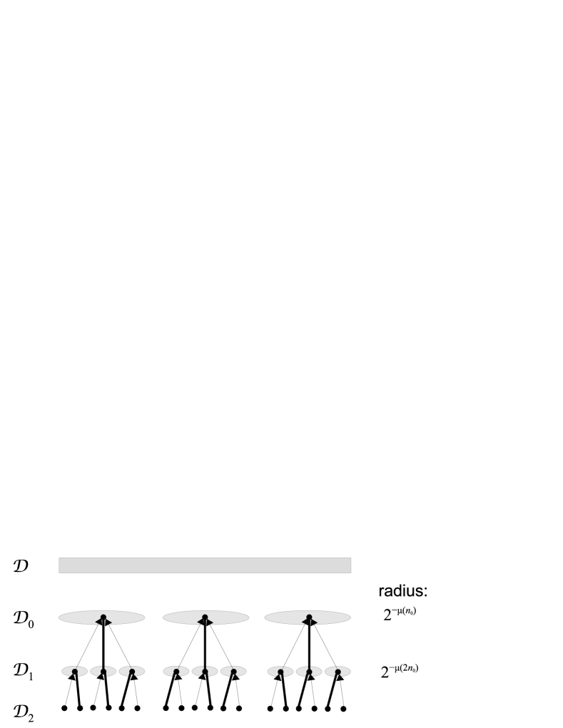
Figure 4: Hierarchical decomposition of the compact ultrametric space $(\mathcal{U},D)$ according to Lemma 7. (Fat dots connected by a bold line segment represent the same point in $\mathcal{U}$.)

Lemma 7

Let $(\mathcal{U},D)$ denote a compact ultrametric space and $\nu:\mathbb{N}\to\mathbb{N}$ be strictly increasing.
Then $\mathcal{U}$ admits a hierarchical cluster decomposition, namely a non-decreasing sequence $\mathcal{U}_{m}\subseteq\mathcal{U}_{m+1}\subseteq\mathcal{U}$ of finite sets with the following properties:

1. The balls $\overline{\operatorname{B}}_{\nu(0)}(x)$, $x\in\mathcal{U}_{0}$, are pairwise disjoint and cover $\mathcal{U}$. More precisely:

   any two distinct $$x,x^{\prime}\in\mathcal{U}_{0} D(x,x^{\prime})>2^{-\nu(0)}$$  have  . (27)

2. For each $m\in\mathbb{N}$ and $x\in\mathcal{U}_{m}$, the balls $\overline{\operatorname{B}}_{\nu(m+1)}(x^{\prime})$, $x^{\prime}\in\overline{\operatorname{B}}_{\nu(m)}(x)\cap\mathcal{U}_{m+1}$, partition $\overline{\operatorname{B}}_{\nu(m)}(x)$. More precisely, for any distinct $x^{\prime},x^{\prime\prime}\in\mathcal{U}$,

   $$x^{\prime},x^{\prime\prime}\in\overline{\operatorname{B}}_{\nu(m)}(x)\cap\mathcal{U}_{m+1}\quad\text{implies}\quad 2^{-\nu(m+1)}<D(x^{\prime},x^{\prime\prime})\leq 2^{-\nu(m)}$$ (28)

Such a decomposition can be constructed by inductive application of Observation 2.2: pick and include in $\mathcal{U}_{m+1}$ precisely one representative center $x^{\prime}$ of all mutually equal balls $\overline{\operatorname{B}}_{\nu(m+1)}(x^{\prime})$, $x^{\prime}\in\overline{\operatorname{B}}_{\nu(m)}(x)$; see Figure 4.

Proof (Theorem 3.3)

Abbreviate $\nu(m)=\mu(n_{0}+m\cdot n_{0})$ for $m\in\mathbb{N}$. Consider the hierarchical cluster decomposition $\mathcal{U}_{m}\subseteq\mathcal{U}_{m+1}\subseteq\mathcal{U}$ from Lemma 7. For $x\in\mathcal{U}_{m+1}\setminus\mathcal{U}_{m}$ let $\mathcal{P}(x)\in\mathcal{U}_{m}$ denote its predecessor, that is, the unique $x^{\prime}=\mathcal{P}(x)\in\mathcal{U}_{m}$ with $2^{-\nu(m+1)}<D(x,x^{\prime})\leq 2^{\nu(m)}$. This mapping $\mathcal{P}$ extends to $\bigcup_{m}\mathcal{U}_{m}\setminus\mathcal{U}_{0}$. Note that $\mathcal{P}(\mathcal{P}(x))$ may be undefined, namely in case $\mathcal{P}(x)\in\mathcal{U}_{0}$. For $x\in\mathcal{U}_{m+1}\setminus\mathcal{U}_{m}$, let

$$\vec{\mathcal{P}}(x)\;:=\;\big{(}\,\mathcal{P}^{(k)}(x)\,,\,\mathcal{P}^{(k-1)}(x)\,,\,\ldots\,,\,\mathcal{P}(\mathcal{P}(x))\,,\,\mathcal{P}(x),x\,\big{)}$$ (29)

abbreviate the sequence of iterated predecessors, reversed. Here $|\vec{\mathcal{P}}(x)|=k\leq m+1$ is the unique natural number such that $k$-fold application $\mathcal{P}^{(k)}(x)\in\mathcal{U}_{0}$. Again note that the sequence (29) may ‘skip’ some levels, i. e., the length $k$ may be (much) shorter than $m$. To $\vec{x}:=\vec{\mathcal{P}}(x)$ choose $(n_{1},\ldots,n_{k})=\vec{n}(x)\in\mathbb{N}$ maximal with $D(x_{j},x_{j-1})\leq 2^{-\mu(n_{j})}$: Then Equation (27) implies $n_{1}\geq n_{0}$ and $n_{j}\geq n_{j-1}+n_{0}$ for $j=2,\ldots k$; hence the prerequisite of Equation (26) is satisfied.

Next we construct a sequence of total single-valued functions $g_{m}:\mathcal{U}_{m}\to\mathcal{V}$ with the following properties:

1. $g_{m+1}|_{\mathcal{U}_{m}}=g_{m}$

2. $g_{m}$ has modulus of continuity $n\mapsto\mu(n+n_{0}-1)$

3. $g_{m}\subseteq G$ as graphs, i. e. $g_{m}$ is a selection of the restriction $G|_{\mathcal{U}_{m}}$.

These $g_{m}$ thus converge uniformly to some total function $g\subseteq G$ on $\mathcal{U}$ with modulus of continuity $\mu(n+n_{0}-1)$.

To obtain $(g_{m})$, employ the (discontinuous) Skolem functions $G_{k}:\subseteq\mathcal{U}^{k+1}\times\mathbb{N}^{k}\to\mathcal{V}$ from Lemma 6: Define $g_{0}(x)=G_{0}(x)$ for $x\in\mathcal{U}_{0}$; and inductively, for $x\in\mathcal{U}_{m+1}\setminus\mathcal{U}_{m}$, define $g_{m+1}(x)=G_{k}\big{(}\vec{\mathcal{P}}(x),\vec{n}(x)\big{)}$ with $k=|\vec{\mathcal{P}}(x)|$. As recorded above, $\vec{\mathcal{P}}(x)$ and $\vec{n}(x)$ together satisfy the prerequisite of Equation (26); hence $g_{m+1}$ is well-defined and satisfies (i) and (iii) by inductive construction.

Concerning (ii), observe that $g_{0}$ has sequential modulus of continuity $\mu$: simply because the prerequisite of Equation (3) with $n\geq n_{0}$ is not satisfied according to Equation (27).

Regarding the induction step $g_{m}\mapsto g_{m+1}$, first consider $x\in\mathcal{U}_{m+1}\setminus\mathcal{U}_{m}$ and $x:=\mathcal{P}(x^{\prime})$: $2^{-\nu(m+1)}<D(x,x^{\prime})\leq 2^{-\nu(m)}=2^{-\mu(n_{0}+mn_{0})}$ as recorded above implies $E(y,y^{\prime})\leq 2^{-(m+1)n_{0}}$ for $y=g_{m+1}(x)=G_{k}\big{(}\vec{\mathcal{P}}(x),\vec{n}(x)\big{)}$ and $y^{\prime}=g_{m+1}(x^{\prime})=G_{k-1}\big{(}\vec{\mathcal{P}}(x^{\prime}),\vec{n}(x^{\prime})\big{)}$, $k=|\vec{\mathcal{P}}(x)|$.

Next consider $x^{\prime},x^{\prime\prime}\in\mathcal{U}_{m+1}\setminus\mathcal{U}_{m}$: If $2^{-\nu(m+1)}<D(x^{\prime},x^{\prime\prime})\leq 2^{-\nu(m)}=2^{-\mu((m+1)n_{0})}$, then $2^{-\nu(m+1)}<D(x^{\prime},x),D(x^{\prime\prime},x)\leq 2^{-\nu(m)}$ for $x:=\mathcal{P}(x^{\prime})=\mathcal{P}(x^{\prime\prime})\in\mathcal{U}_{m}$ according to Equation (28); hence $E(y^{\prime},y^{\prime\prime})\leq\max\{E(y^{\prime},y),E(y,y^{\prime\prime})\}\leq 2^{-(m+1)n_{0}}$ for $y=g_{m+1}(x)$, $y^{\prime}=g_{m+1}(x^{\prime})$, $y^{\prime\prime}=g_{m+1}(x^{\prime\prime})$ as before. Note that $D(x^{\prime},x^{\prime\prime})\leq 2^{-\mu(n)}$ in case $(m+2)n_{0}>n>(m+1)n_{0}$ does not imply $D(x^{\prime},x),d(x^{\prime\prime},x)\leq 2^{-\mu(n)}$; hence here we only obtain modulus $n\mapsto\mu(n+n_{0}-1)$ instead of $\mu(n)$. Note that this case cannot occur over (a subset of) Cantor space $\mathcal{C}$ as domain, though.

Finally suppose $x,x^{\prime}\in\mathcal{U}_{m+1}\setminus\mathcal{U}_{m}$ have $2^{-\nu(m)}<D(x,x^{\prime})\leq 2^{-\nu(m^{\prime})}$. Then $x^{\prime\prime}:=\mathcal{P}(x)\in\mathcal{U}_{m}$ and $x^{\prime\prime\prime}:=\mathcal{P}(x^{\prime})\in\mathcal{U}_{m}$ have $D(x^{\prime\prime},x^{\prime\prime\prime})=D(x,x^{\prime})$ by Equation (28) and Observation 2.2iv); and $2^{-\nu(m+1)}<D(x,x^{\prime\prime}),D(x^{\prime},x^{\prime\prime\prime})\leq 2^{-\nu(m)}$ as recorded above. Hence $y:=g_{m+1}(x)$, $y^{\prime}:=g_{m+1}(x^{\prime})$, $y^{\prime\prime}:=g_{m+1}(x^{\prime\prime})$, $y^{\prime\prime\prime}:=g_{m+1}(x^{\prime\prime\prime})$ have $E(y,y^{\prime\prime}),E(y^{\prime},y^{\prime\prime\prime})\leq 2^{-(m+1)n_{0}}$ as before; and $E(y^{\prime\prime},y^{\prime\prime\prime})\leq 2^{-(m^{\prime}+1)n_{0}}$ by induction hypothesis: Together $E(y,y^{\prime})\leq\max\{E(y,y^{\prime\prime}),E(y^{\prime\prime},y^{\prime\prime\prime}),E(y^{\prime\prime\prime},y^{\prime})\}\leq 2^{-(m^{\prime}+1)n_{0}}$: concluding the final case of the induction step to verify (ii). ∎

Proof (Example 8)

1. Let $n_{0}\in\mathbb{N}$ such that $2^{-n_{0}+1}<\varepsilon$. If $x_{0}\leq 0$ take $y_{0}:=0\in h_{\varepsilon}(x_{0})$, otherwise take $y_{0}:=1\in h_{\varepsilon}(x_{0})$: Equation (25) shows $x_{k}<\varepsilon$ and hence $y_{k}:=0\in h_{\varepsilon}(x_{k})$.

2. Let us call an integer sequence $(a_{n})_{{}_{n\geq 1}}$ a $\widetilde{\delta}$-name of $x\in[0;1]$ iff $\big{(}\mathrm{bin}_{n}(a_{n}):n\geq 1\big{)}\in\mathcal{C}$ is a $\delta$-name of $x$. Note that (only) here, the index starts with $1$ instead of $0$. Since $\mu(n)=n+2$, Equation (25) improves:

   $$d(x_{\ell},x_{k})\;\leq\;\sum\nolimits_{j=\ell+1}^{k}2^{-(n_{j}+2)}\;\leq\;2^{-n_{\ell+1}-1}\enspace.$$ (30)

   
   

   To $x_{0}\in[0;1]$ consider the integer sequence $\bar{y}_{0}=(y^{(0)}_{n})_{{}_{n}}=\big{(}\lfloor 2^{n}\cdot x_{0}\rceil_{n}\big{)}$. Since $|y^{(0)}_{n}-x_{0}|\leq 2^{-n-1}$, and with $|x_{0}-x_{k}|\leq 2^{-n_{1}-1}$ according to Equation (30), the $n_{1}$-element sequence $(y^{(0)}_{1},\ldots,y^{(0)}_{n_{1}})$ extends to $\widetilde{\delta}$-names of any $x_{k}$. More precisely, $\bar{y}^{(1)}=(y^{(1)}_{n})_{{}_{n}}:=\big{(}\lfloor 2^{n}\cdot x_{1}\rceil_{n}\big{)}$ for $n>n_{1}$ and $y^{(1)}_{n}:=y^{(0)}_{n}$ for $n\leq n_{1}$ constitutes a $\widetilde{\delta}$-name of $x_{1}$: agreeing on the first $n_{1}$ entries; and now with the property $|y^{(1)}_{n}-x_{1}|\leq 2^{-n-1}$ for all $n>n_{1}$; which, together with $|x_{1}-x_{k}|\leq 2^{-n_{2}-1}$ makes $(y^{(0)}_{1},y^{(0)}_{n_{1}},y^{(1)}_{n_{1}+1},y^{(1)}_{n_{2}})$ extend to $\widetilde{\delta}$-names of any $x_{k}$, $k>1$. And so forth: yielding a sequence of $\widetilde{\delta}$-names $\bar{y}^{(k)}\in\mathbb{N}^{\mathbb{N}}$ of $x_{k}\in\overline{\operatorname{B}}_{n_{k}+2}(x_{k-1})$ which agree on the first $n_{k}$ entries. These in turn yield $\delta$-names $y_{k}\in\delta^{-1}(x_{k})\subseteq\mathcal{C}$ which agree on the first $\nu(k_{k}):=\sum_{j<n_{k}}j=n_{k}\cdot(n_{k}+1)/2\geq n_{k}$ bits: recall Example 4. In particular $y_{k}\in\overline{\operatorname{B}}_{n_{k}}(y_{k-1})$.

3. We basically iterate the proof of Example 5(iii): Consider any $\vec{b}^{(0)}=\big{(}b_{0}^{(0)},\ldots,b_{n_{1}-1}^{(0)}\big{)}\in\{-1,0,1\}^{n_{1}}$ with $|x_{0}-\mathrm{sbin}(\vec{b}^{(0)})|\leq 2^{-n_{1}-1}$: such that it extends to signed binary expansions of any $x_{k}$, since $|x_{0}-x_{k}|\leq 2^{-n_{1}-1}$ according to Equation (30). In particular the signed binary expansion of $\tfrac{1}{2}+(x_{1}-x_{0})\cdot 2^{n_{1}+1}\in[0;1]$ yields $\big{(}b_{n_{1}}^{(1)},\ldots,b_{n_{2}-1}^{(1)}\big{)}\in\{-1,0,1\}^{n_{2}-n_{1}}$ such that

   $$\vec{b}^{(1)}\;:=\;\big{(}b_{0}^{(0)},\ldots,b_{n_{1}-1}^{(0)},b_{n_{1}}^{(1)},\ldots,b_{n_{2}-1}^{(1)}\big{)}\in\{-1,0,1\}^{n_{2}}$$

   has $|x_{1}-\mathrm{sbin}(\vec{b}^{(1)})|\leq 2^{-n_{2}-1}$; hence, in view of $|x_{1}-x_{k}|\leq 2^{-n_{2}-1}$ according to Equation (30), $\vec{b}^{(1)}$ extends to signed binary expansions of any $x_{k}$, $k>1$. And so forth: yielding a sequence of $\sigma$-names $\bar{y}^{(k)}\in\mathcal{C}$ of $x_{k}\in\overline{\operatorname{B}}_{n_{k}+2}(x_{k-1})$ which agree on the first $n_{k}$ bits: $\bar{y}^{(k)}\in\overline{\operatorname{B}}_{n_{k}}(\bar{y}^{(k-1)})$. ∎

3.5 Representations over Compact Ultrametric Spaces

Motivated by Example 1, Subsection 1.3 had considered representations over domains beyond Cantor space. And Theorem 3.3 suggests which domains seem suitable for complexity considerations: ‘almost’ homogeneous compact ultrametric spaces.

The present section extends our notions of quantitative admissibility (Section 2) from representations over Cantor space to arbitrary compact ultrametric domains: based on quantitative continuity of multifunctions according to Definition 5. We then establish a quantitative Main Theorem for multifunctions.

Let us first generalize Definition 2 from Cantor space with entropy $\operatorname{id}$ by Lemma 3a), following the generic approach from Remark 3.

Definition 6

Fix compact ultrametric space $(\mathcal{U},D)$ with entropy $\mathcal{H}$.

1. For (single-valued) representations $\xi:\subseteq\mathcal{U}\twoheadrightarrow X$ and $\upsilon:\subseteq\mathcal{V}\twoheadrightarrow Y$, a $(\xi,\upsilon)$-realizer of a multifunction $f:X\rightrightarrows Y$ is a (single-valued) mapping $F:\subseteq\mathcal{U}\to\mathcal{V}$ satisfying any/all of the conditions from Observation 3.1c).

2. Call representation $\xi:\subseteq\mathcal{U}\twoheadrightarrow X$ polynomially admissible  iff  it satisfies (b i) and (b ii), where:

3. $\xi$ has modulus of continuity $\mu$ such that $\mathcal{H}\circ\mu\leq\eta\circ\operatorname{poly}$.

4. Every continuous surjective $\xi^{\prime}:\subseteq\mathcal{U}\twoheadrightarrow X$ has $\xi^{\prime}\preccurlyeq_{\rm P}\xi$.

5. Call representation $\xi:\subseteq\mathcal{U}\twoheadrightarrow X$ polynomially standard  iff  it satisfies (b i) $\mathcal{H}\circ\mu\leq\eta\circ\operatorname{poly}$ and (b ii’) $\xi^{\prime}\preccurlyeq_{\rm P}\xi$ for every (not necessarily surjective) $\xi^{\prime}:\subseteq\mathcal{U}\to X$ and the following condition (c i):

6. $d(x,x^{\prime})\leq 2^{-\operatorname{poly}(n)}$ implies $d_{\xi}(x,x^{\prime})\leq 2^{-\mu(n)}$.

7. Call representation $\xi:\subseteq\mathcal{U}\twoheadrightarrow X$ linearly admissible  iff  it satisfies (d i) and (d ii), where:

8. $\xi$ has modulus of continuity $\mu$ with $\mathcal{H}\circ\mu\leq\eta\circ\mathcal{O}$.

9. Every continuous surjective $\xi^{\prime}:\subseteq\mathcal{U}\twoheadrightarrow X$ has $\xi^{\prime}\preccurlyeq_{\rm L}\xi$.

10. Call representation $\xi:\subseteq\mathcal{U}\twoheadrightarrow X$ linearly standard  iff  it satisfies (d i) $\mathcal{H}\circ\mu\leq\eta\circ\mathcal{O}$ and (d ii’) $\xi^{\prime}\preccurlyeq_{\rm L}\xi$ for every (not necessarily surjective) $\xi^{\prime}:\subseteq\mathcal{U}\to X$ and the following condition (e i):

11. $d(x,x^{\prime})\leq 2^{-\mathcal{O}(n)}\quad\Rightarrow\quad d_{\xi}(x,x^{\prime})\leq 2^{-\mu(n)}$.

Note that, compared to Definition 2, $\eta$ has been replaced with $\mu$ in Items (c i) and (e i): which over Cantor space $\mathcal{U}=\mathcal{C}$ with $\mathcal{H}=\operatorname{id}$ makes no difference because of (b i) and (d i), but for generic $\mathcal{U}$ turns out as more convenient. It does affect Items (b) of the following generalized Theorem 2.1, though:

Theorem 3.4

Fix compact ultrametric space $(\mathcal{U},D)$ with entropy $\mathcal{H}$.

1. Suppose $(X,d)$ admits a polynomially standard representation $\xi:\subseteq\mathcal{U}\twoheadrightarrow X$ and $\xi^{\prime}:\subseteq\mathcal{U}\twoheadrightarrow X$ is polynomially admissible. Then $\xi^{\prime}$ is polynomially standard, too.

2. Suppose $(X,d)$ admits a linearly standard representation $\xi:\subseteq\mathcal{U}\twoheadrightarrow X$ and $\xi^{\prime}:\subseteq\mathcal{U}\twoheadrightarrow X$ is linearly admissible. Then $\xi^{\prime}$ is linearly standard, too.

3. Fix a polynomially standard representation $\xi:\subseteq\mathcal{U}\twoheadrightarrow X$ of metric space $(X,d)$ with entropy $\eta$. Consider $f:X\to Y$ for metric space $(Y,e)$. If $f\circ\xi$ has modulus of continuity $\boldsymbol{\mu}\circ\lambda$, then $f$ has modulus of continuity $\operatorname{poly}\circ\lambda$.

4. If $\xi:\subseteq\mathcal{U}\twoheadrightarrow X$ is linearly standard, then $f$ has modulus of continuity $\mathcal{O}\circ\lambda$.

5. Let $\xi:\subseteq\mathcal{U}\twoheadrightarrow X$ and $\upsilon:\subseteq\mathcal{U}\twoheadrightarrow Y$ denote representations of metric spaces $(X,d)$ and $(Y,e)$ with respective entropies $\eta$ and $\theta$.

6. Suppose $\xi$ and $\upsilon$ are polynomially standard. Consider $f:X\to Y$ with modulus of continuity $\lambda$. Then $f$ admits a $(\xi,\upsilon)$-realizer $F:\operatorname{dom}(\xi)\to\operatorname{dom}(\upsilon)$ with modulus of continuity $\Lambda$ such that $\mathcal{H}\circ\Lambda\circ\mathcal{H}\circ\theta\leq\eta\circ\operatorname{poly}\circ\lambda\circ\operatorname{poly}$.

7. Suppose $\xi$ and $\upsilon$ are linearly standard. Consider $f:X\to Y$ with modulus of continuity $\lambda$. Then $f$ admits a $(\xi,\upsilon)$-realizer $F$ with modulus of continuity $\Lambda$ such that $\mathcal{H}\circ\Lambda\circ\mathcal{H}\circ\theta\leq\eta\circ\mathcal{O}\circ\lambda\circ\mathcal{O}$.

8. Let $\xi:\subseteq\mathcal{U}\twoheadrightarrow X$ and $\upsilon:\subseteq\mathcal{U}\twoheadrightarrow Y$ denote representations of metric spaces $(X,d)$ and $(Y,e)$ with respective entropies $\eta$ and $\theta$.

9. Suppose $\xi$ and $\upsilon$ are polynomially standard. Let $f:X\to Y$ admit a $(\xi,\upsilon)$-realizer $F$ with modulus of continuity $\mathcal{H}^{\underline{-1}}\circ\eta\circ\lambda$. Then $f$ has modulus of continuity $\operatorname{poly}\circ\lambda\circ\mathcal{H}^{\underline{-1}}\circ\theta\circ\operatorname{poly}$.

10. Suppose $\xi$ and $\upsilon$ are linearly standard. Let $f:X\to Y$ admit a $(\xi,\upsilon)$-realizer $F$ with modulus of continuity $\mathcal{H}^{\underline{-1}}\circ\eta\circ\lambda$. Then $f$ has modulus of continuity $\mathcal{O}\circ\lambda\circ\mathcal{H}^{\underline{-1}}\circ\theta\circ\mathcal{O}$.

Note that for Cantor space $\mathcal{U}=\mathcal{C}$ with $\mathcal{H}=\operatorname{id}$ Theorem 3.4 recovers Theorem 2.1.

We can now generalize Theorem 2.3. Theorem 3.4 supposes that the space(s) under consideration be equipped with linearly/polynomially standard representations to begin with. It remains to show that many spaces actually do admit such representations:

Theorem 3.5

Fix a compact ultrametric space $(\mathcal{U},D)$ with minimum relative binary capacity $\mathcal{K}=\mathcal{K}_{m}(n)$. Fix a compact metric space $(X,d)$ with binary entropy $\eta$, and a strictly increasing positive integer sequence $n_{k}$, $k\in\mathbb{N}$. Inductively define $\mu(0):=\mathcal{K}^{\underline{-1}}\circ\eta(1+n_{0})$ and

$$\mu(n)\;:=\;\mathcal{K}_{\mu(n_{k})}^{\underline{-1}}\circ\eta_{n_{k}}\big{(}1+n_{k+1}\big{)}\;\in\;\mathbb{N}\quad\text{ for }n_{k}<n\leq n_{k+1}\enspace.$$ (31)

1. Suppose that it holds

   $$n_{K+1}\leq\mathcal{O}(n_{K})\quad\text{and}\quad\mu(n_{K})\;\leq\;\mathcal{K}^{\underline{-1}}\big{(}\eta(\mathcal{O}(n_{K}))\big{)}$$

   with respect to asymptotics $K\to\infty$ but ignoring constants depending on $(n_{k})$. Then there exists linearly admissible $\xi:\subseteq\mathcal{U}\twoheadrightarrow X$ with modulus of continuity $\mu$.

2. Suppose $\displaystyle n_{K+1}\leq\operatorname{poly}(n_{K})\quad\text{and}\quad\mu(n_{K})\;\leq\;\mathcal{K}^{\underline{-1}}\big{(}\eta(\operatorname{poly}(n_{K}))\big{)}$ with respect to asymptotics $K\to\infty$ but ignoring constants depending on $(n_{k})$. Then there exists polynomially admissible $\xi:\subseteq\mathcal{U}\twoheadrightarrow X$ with modulus of continuity $\mu$.

Recall (Example 7a) that Cantor space $\mathcal{U}:=\mathcal{C}$ has $\mathcal{K}_{m}(n)=\max\{n-1-m,0\}$; hence $\mathcal{K}_{m}^{\underline{-1}}(N)=N+1+m$ and

$$\mu(n_{K+1})\;=\;\eta_{n_{K}}\big{(}1+n_{K+1}\big{)}\>+\>1\>+\>\mu(n_{K})\;=\cdots=\;\eta\big{(}1+n_{0})\>+\>\sum\nolimits_{k=0}^{K}\eta_{n_{k}}\big{(}1+n_{k+1}\big{)}\>+\>(K+1)$$

(almost) recovering Theorem 2.3.

The proof of Theorem 3.5 is similar to that of Theorem 2.3 on pages 2.4ff, with the following changes: Recall the induction step $\xi_{K}\mapsto\xi_{K+1}$ with the mapping $\xi_{K}:\subseteq\{\textup{{0}},\textup{{1}}\}^{m_{K}}\to X$ satisfying conditions (I) and (II). Defined inductively on Cantor space, $m_{K+1}:=m_{K}+\eta_{n_{K}}\big{(}1+n_{K+1}\big{)}$ guarantees $\operatorname{dom}(\xi_{K+1})$ to

1. contain sufficiently many initial segments to encode the $\leq 2^{m_{K+1}}$ centers of balls of radius $2^{-n_{K+1}-1}$ covering $\overline{\operatorname{B}}_{n_{K}}$ according to (I);

2. encode in a discernible way in that these initial segments (or rather: their extensions) have pairwise distances $>2^{-m_{K+1}}$

and hence trivially satisfy the modulus condition (3), while (II) makes sure that this property carries over to the induction step.

Generalizing Cantor space $\mathcal{C}$ to $\mathcal{U}$, initial segments are replaced by points witnessing the capacity: such that, in addition to unmodified (I) and (II),

1. $\operatorname{dom}(\xi_{K+1})\subseteq\mathcal{U}$ has cardinality $\geq 2^{m_{K+1}}$

2. and any two points in $\operatorname{dom}(\xi_{K+1})$ have pairwise distances $>2^{-\mu(n_{K+1})}$

and hence again trivially satisfy the modulus condition (3) with $\mu$ according to Equation (31): Note that arguments in $\overline{\operatorname{B}}_{m_{K}}(x)\subseteq\mathcal{U}$ having pairwise distance $>2^{-\mu(n_{K+1})}$ from each other also have such distance to arguments in $\overline{\operatorname{B}}_{\mu(n_{K})}(x^{\prime})$ for $D(x,x^{\prime})>2^{-\mu(n_{K})}$ due to $(\mathcal{U},D)$ being ultrametric. ∎

Proceeding from Cantor to other ultrametric spaces provides a promising approach to the open problem of defining (!) computational complexity for higher types [Roy99]:

Example 9

Returning to Example 1, consider the application functional

$$\operatorname{App}\;:\;\operatorname{Lip}_{1}([0;1],[0;1])\times[0;1]\;\ni\;(f,x)\;\mapsto\;f(x)\;\in\;[0;1]$$

which is non-expansive i. e. 1-Lipschitz. According to Lemma 3e+f), no Cantor space representation of $[0;1]^{\dagger}=\operatorname{Lip}_{1}([0;1],[0;1])$ can have a sub-exponential modulus of continuity.

In fact, for every $\Delta:\subseteq\mathcal{C}\twoheadrightarrow[0;1]^{\dagger}=\operatorname{Lip}_{1}([0;1],[0;1])$ and with the Cartesian product representation $\Delta\times\delta$ of $[0;1]^{\dagger}\times[0;1]$, no $(\Delta\times\delta,\delta)$-realizer $F:\subseteq\mathcal{C}\to\mathcal{C}$ can have a sub-exponential modulus of continuity: the seemingly simple application functional is not computable in polynomial time—when using Cantor space representations.

The representation $\delta_{\square}$ from [KC12, §3.4] on the other hand is (or more precisely: can be rewritten and restricted to be) defined over the compact ultrametric space $\mathcal{U}:=(\{\textup{{0}},\textup{{1}}\}^{*})^{\dagger}$, which according to Example 7b) has exponential binary entropy $\mathcal{H}(n)=2^{n}$ and relative binary capacity $\mathcal{K}_{m}(n)=2^{n-1}-2^{m}$ for $n>m$. Hence, over $(\{\textup{{0}},\textup{{1}}\}^{*})^{\dagger}$ instead of $\mathcal{C}$, Lemma 3e+f) does not prohibit a representation of $[0;1]^{\dagger}$ from having polynomial modulus of continuity. And indeed, $\operatorname{App}$ is $(\delta_{\square}\times\delta,\delta)$-computable in polynomial time [KC12, Lemma 4.9].

4 Concluding Comments

The present work has boiled down the original Question 1 to Definition 2, thoroughly justified with the many benefits of this new notion of quantitative admissibility: existence (Theorem 2.3) and closure properties (Theorem 2.4) and quantitative strengthenings (Theorems 2.1) of the classical qualitative Main Theorem (Fact 1.1) that generalize and systematize (Theorem 3.4) previous results about known ad-hoc encodings (Corollary 1).

It remains to further investigate the following purely mathematical question:

Question 2

What are sufficiently ‘rich’ classes/categories of compact metric spaces $(X,d)$ with relative binary entropy $\eta=\eta_{m}(n)$ which admit linearly/polynomially admissible/standard representations in the sense of Definition 2?

What are sufficiently ‘rich’ classes/categories of compact metric spaces that satisfy the hypothesis of Theorem 2.3, i. e., for which there exist strictly increasing positive integer sequences $n_{k}$ such that $\mu(n_{K}):=\eta(1+n_{0})+\sum_{k=0}^{K}\eta_{n_{k}}\big{(}1+n_{k+1}\big{)}$ satisfies

1. $n_{k+1}\leq\mathcal{O}(n_{k})$ and

2. $\mu(n_{K})\leq\eta_{X}\big{(}\mathcal{O}(n_{K})\big{)}$ ?

Throughout this work we have focused on representing compact metric spaces $(X,d)$. These admit complexity analyses in dependence on one integer parameter $n$ only; cmp. [Sch04]. Generalizing to sigma-compact metric spaces $X=\bigcup_{k}X_{k}$ with compact $X_{k}$ leads to parameterized complexity, with additional dependence on secondary parameter $k\in\mathbb{N}$ [NS20].

References

- [BBS04] Andrej Bauer, Lars Birkedal, and Dana S. Scott. Equilogical spaces. Theoretical Computer Science, 315:35–59, 2004.
- [BC98] Daniela Bertacchi and Camillo Costantini. Existence of selections and disconnectedness properties for the hyperspace of an ultrametric space. Topology and its Applications, 88(3):179 – 197, 1998.
- [BCSS98] Leonore Blum, Felipe Cucker, Mike Shub, and Steve Smale. Complexity and Real Computation. Springer, 1998.
- [BH94] Vasco Brattka and Peter Hertling. Continuity and computability of relations, 1994.
- [dBvKOC08] Marc de Berg, Marc van Kreveld, Marc Overmars, and Otfried Cheong. Computational Geometry. Springer, 3rd edition, 2008.
- [DK89] D. Du and Ker-I Ko. Computational complexity of integration and differentiation of convex functions. System Sci. and Math. Sci., 2:70–79, 1989.
- [Fri84] Harvey Friedman. On the computational complexity of maximization and integration. Advances in Mathematics, 53:80–98, 1984.
- [Grz57] Andrzej Grzegorczyk. On the definitions of computable real continuous functions. Fundamenta Mathematicae, 44:61–71, 1957.
- [HHW55] Cecil Hastings, Jeanne T. Hayward, and James P. Wong. Approximations for Digital Computers. Princeton University Press, 1955.
- [IM04] Piotr Indyk and Jirí Matousek. Low-distortion embeddings of finite metric spaces. In Jacob E. Goodman and Joseph O’Rourke, editors, Handbook of Discrete and Computational Geometry, Second Edition, pages 177–196. Chapman and Hall/CRC, 2004.
- [JHG88] J.F.Traub, H.Woźniakowski, and G.W.Wasilkowski. Information-Based Complexity. Academic Press, 1988.
- [Kaw10] Akitoshi Kawamura. Lipschitz continuous ordinary differential equations are polynomial-space complete. Computational Complexity, 19(2):305–332, 2010.
- [KC12] Akitoshi Kawamura and Stephen Cook. Complexity theory for operators in analysis. ACM Transactions on Computation Theory, 4:2(5), 2012.
- [KF82] Ker-I Ko and H. Friedman. Computational complexity of real functions. Theoretical Computer Science, 20:323–352, 1982.
- [KMRZ15] Akitoshi Kawamura, Norbert Müller, Carsten Rösnick, and Martin Ziegler. Computational benefit of smoothness: parameterized bit-complexity of numerical operators on analytic functions and Gevrey’s hierarchy. J. Complexity, 31(5):689–714, 2015.
- [Ko91] Ker-I Ko. Complexity Theory of Real Functions. Progress in Theoretical Computer Science. Birkhäuser, Boston, 1991.
- [KO14] Akitoshi Kawamura and Hiroyuki Ota. Small complexity classes for computable analysis. In Mathematical foundations of computer science 2014. Part II, volume 8635 of Lecture Notes in Comput. Sci., pages 432–444. Springer, Heidelberg, 2014.
- [Koh08] Ulrich Kohlenbach. Applied Proof Theory: Proof Interpretations and their Use in Mathematics. Springer, Berlin, 2008.
- [KSZ16] Akitoshi Kawamura, Florian Steinberg, and Martin Ziegler. Complexity theory of (functions on) compact metric spaces. In Proceedings of the 31st Annual ACM/IEEE Symposium on Logic in Computer Science, LICS ’16, New York, NY, USA, July 5-8, 2016, pages 837–846, 2016.
- [KT59] A.N. Kolmogorov and V.M. Tikhomirov. -entropy and -capacity of sets in functional spaces. Uspekhi Mat. Nauk, 14(2):3–86, 1959.
- [KW85] Christoph Kreitz and Klaus Weihrauch. Theory of representations. Theoretical Computer Science, 38:35–53, 1985.
- [Lim19] Donghyun Lim. Representations of totally bounded metric spaces and their computational complexity. Master’s thesis, KAIST, School of Computing, 2019.
- [LP20] Donghyun Lim and Sewon Park. Topological aspects on nondetermistic computation. In Proc. Korea Software Congress 2020 (KSC), Proceedings of Korean Institute of Information Scientists and Engineers (한국정보과학회 학술발표논문집), Seoul, South Korea, December 2020. Korean Institute of Information Scientists and Engineers.
- [Luc77] Horst Luckhardt. A fundamental effect in computations on real numbers. Theoretical Computer Science, 5(3):321–324, 1977.
- [LZ20] Donghyun Lim and Martin Ziegler. Quantitative coding and complexity theory of compact metric spaces. In Marcella Anselmo, Gianluca Della Vedova, Florin Manea, and Arno Pauly, editors, Beyond the Horizon of Computability - 16th Conference on Computability in Europe, CiE 2020, Fisciano, Italy, June 29 - July 3, 2020, Proceedings, volume 12098 of Lecture Notes in Computer Science, pages 205–214. Springer, 2020.
- [MdB19] Matthias Schröder Matthew de Brecht, Arno Pauly. Overt choice. Computability, Preprint:1–23, 2019.
- [Mül86] Norbert Th. Müller. Subpolynomial complexity classes of real functions and real numbers. In Laurent Kott, editor, Proceedings of the 13th International Colloquium on Automata, Languages, and Programming, volume 226 of Lecture Notes in Computer Science, pages 284–293, Berlin, 1986. Springer.
- [NS20] Eike Neumann and Florian Steinberg. Parametrised second-order complexity theory with applications to the study of interval computation. Theor. Comput. Sci., 806:281–304, 2020.
- [PB97] Amin Shokrollahi Peter Bürgisser, Michael Clausen. Algebraic Complexity Theory, volume 315 of Grundlehren der mathematischen Wissenschaften. Springer, 1997.
- [PSZ20] Arno Pauly, Dongseong Seon, and Martin Ziegler. Computing haar measures. In Maribel Fernández and Anca Muscholl, editors, 28th EACSL Annual Conference on Computer Science Logic, CSL, volume 152 of LIPIcs, pages 34:1–34:17. Schloss Dagstuhl - Leibniz-Zentrum für Informatik, 2020.
- [PZ13] Arno Pauly and Martin Ziegler. Relative computability and uniform continuity of relations. Journal of Logic and Analysis, 5(7):1–39, 2013.
- [Roy99] James S. Royer. A list of papers on computational complexity at higher types, 1999.
- [RS14a] Dušan Repovš and Pavel V. Semenov. Continuous selections of multivalued mappings. In K.P. Hart, J. van Mill, and P. Simon, editors, Recent Progress in General Topology III, pages 711–749. Atlantis Press, 2014.
- [RS14b] Luca Motto Ross and Philipp Schlicht. Lipschitz and uniformly continuous reducibilities on ultrametric Polish spaces, volume 4 of Ontos Mathematical Logic, pages 213–258. De Gruyter, 2014.
- [Sch01] Matthias Schröder. Admissible representations of limit spaces. In Jens Blanck, Vasco Brattka, and Peter Hertling, editors, Computability and Complexity in Analysis, volume 2064 of Lecture Notes in Computer Science, pages 273–295, Berlin, 2001. Springer. 4th International Workshop, CCA 2000, Swansea, UK, September 2000.
- [Sch02] Matthias Schröder. Extended admissibility. Theoretical Computer Science, 284(2):519–538, 2002.
- [Sch04] Matthias Schröder. Spaces allowing type-2 complexity theory revisited. Mathematical Logic Quarterly, 50(4,5):443–459, 2004.
- [Sch06] Matthias Schröder. Admissible representations in computable analysis. In Logical Approaches to Computational Barriers, Second Conference on Computability in Europe, CiE 2006, Swansea, UK, June 30-July 5, 2006, Proceedings, pages 471–480, 2006.
- [Sch07] Matthias Schröder. Admissible representations of probability measures. In Douglas Cenzer, Ruth Dillhage, Tanja Grubba, and Klaus Weihrauch, editors, Proceedings of the Third International Conference on Computability and Complexity in Analysis, volume 167 of Electronic Notes in Theoretical Computer Science, pages 61–78, Amsterdam, 2007. Elsevier. CCA 2006, Gainesville, Florida, USA, November 1–5, 2006.
- [Sch20] Matthias Schröder. Admissibly represented spaces and qcb-spaces, 2020.
- [SS17] Matthias Schröder and Florian Steinberg. Bounded time computation on metric spaces and banach spaces. In 32nd Annual ACM/IEEE Symposium on Logic in Computer Science, LICS 2017, Reykjavik, Iceland, June 20-23, 2017, pages 1–12. IEEE Computer Society, 2017.
- [Ste16] Florian Steinberg. Computational Complexity Theory for Advanced Function Spaces in Analysis. PhD thesis, TU Darmstadt, 2016.
- [Ste17] Florian Steinberg. Complexity theory for spaces of integrable functions. Logical Methods in Computer Science, 13(3), 2017.
- [Tur37] Alan M. Turing. On computable numbers, with an application to the “Entscheidungsproblem”. Proceedings of the London Mathematical Society, 42(2):230–265, 1937.
- [Tur38] Alan M. Turing. On computable numbers, with an application to the “Entscheidungsproblem”. A correction. Proceedings of the London Mathematical Society, 43(2):544–546, 1938.
- [Wal82] Peter Walters. An Introduction to Ergodic Theory. Number 79 in Graduate Texts in Mathematics. Springer, 1982.
- [Wei00] Klaus Weihrauch. Computable Analysis. Springer, Berlin, 2000.
- [Wei03] Klaus Weihrauch. Computational complexity on computable metric spaces. Mathematical Logic Quarterly, 49(1):3–21, 2003.
- [Zie03] Martin Ziegler. Computable operators on regular sets. In Vasco Brattka, Matthias Schröder, Klaus Weihrauch, and Ning Zhong, editors, Computability and Complexity in Analysis, volume 302 of Informatik Berichte, pages 389–406. FernUniversität in Hagen, August 2003. International Conference, CCA 2003, Cincinnati, USA, August 28–30, 2003.
- [ZZ99] Ning Zhong and Bing-Yu Zhang. -computability. Mathematical Logic Quarterly, 45(4):449–456, 1999.