Distribution Approximation and Statistical Estimation Guarantees of Generative Adversarial Networks
Abstract
Generative Adversarial Networks (GANs) have achieved a great success in unsupervised learning. Despite its remarkable empirical performance, there are limited theoretical studies on the statistical properties of GANs. This paper provides approximation and statistical guarantees of GANs for the estimation of data distributions that have densities in a Hölder space. Our main result shows that, if the generator and discriminator network architectures are properly chosen, GANs are consistent estimators of data distributions under strong discrepancy metrics, such as the Wasserstein-1 distance. Furthermore, when the data distribution exhibits low-dimensional structures, we show that GANs are capable of capturing the unknown low-dimensional structures in data and enjoy a fast statistical convergence, which is free of curse of the ambient dimensionality.
Our analysis for low-dimensional data builds upon a universal approximation theory of neural networks with Lipschitz continuity guarantees, which may be of independent interest.
Keywords: Generative adversarial networks, Distribution estimation, Low-dimensional data, Universal approximation
1 Introduction
Generative Adversarial Networks (GANs, [1]) utilize two neural networks competing with each other to generate new samples with the same distribution as the training data. They have been successful in many applications including producing photorealistic images, improving astronomical images, and modding video games [2, 3, 4, 5, 6, 7, 8].
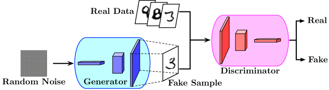
From the perspective of statistics, GANs have stood out as an important unsupervised method for learning target data distributions. Different from explicit distribution estimators, such as the kernel density estimator, GANs implicitly learn the data distribution and act as samplers to generate new fake samples mimicking the data distribution (see Figure 1).
To estimate a data distribution , GANs solve the following minimax optimization problem
| (1) |
where denotes a class of generators, denotes a symmetric class (if , then ) of discriminators, and follows some easy-to-sample distribution , e.g., a uniform distribution. The estimator of is given by a pushforward distribution of under .
The inner maximization problem of (1) is an Integral Probability Metric (IPM, [9]), which quantifies the discrepancy between two distributions and w.r.t. the symmetric function class :
Accordingly, GANs essentially minimize an IPM between the generated distribution and the data distribution. IPM unifies many standard discrepancy metrics. For example, when is taken to be all -Lipschitz functions, is the Wasserstein-1 distance ; when is the class of all indicator functions, is the total variation distance; when is taken as neural networks, is the so-called “neural net distance” [10].
In practical GANs, the generator and discriminator classes and are parametrized by neural networks. We denote and to emphasize such a parameterization. In this paper, we focus on using feedforward ReLU networks, since it has wide applications [11, 12, 13] and can ease the notorious vanishing gradient issue during training, which commonly arises with sigmoid or hyperbolic tangent activations [12, 14]
When samples of the data distribution are given, denoted as , one can replace in (1) by its empirical counterpart , and (1) becomes
| (2) |
where and are parameters in the generator and discriminator networks, respectively. The empirical estimator of given by GANs is the pushforward distribution of under , denoted by .
In contrast to the prevalence of GANs in applications, there are very limited works on the theoretical properties of GANs [10, 15, 16, 17, 18]. This paper focuses on the following fundamental questions from a theoretical point of view:
-
•
(Q1). What types of distributions can be approximated by a deep neural network generator?
-
•
(Q2). If the distribution can be approximated, what is the statistical rate of estimation using GANs?
-
•
(Q3). If further there are unknown low-dimensional structures in the data distribution, can GANs capture the low-dimensional data structure and enjoy a fast rate of estimation?
1.1 Main results
Results in Euclidean space. To address (Q1) and (Q2), we show that, if the generator and discriminator network architectures are properly chosen, GANs can learn distributions with Hölder densities supported on a convex domain. Specifically, we consider a data distribution supported on a compact convex subset , where is the data dimension. We assume has an -Hölder density with respect to Lebesgue measure in and the density is lower bounded away from on .
Our generator and discriminator network architectures are explicitly chosen — we specify the width and depth of the network, total number of neurons, and total number of weight parameters (details are provided in Section 3). Roughly speaking, the generator needs to be flexible enough to approximately transform an easy-to-sample distribution to the data distribution, and the discriminator is powerful enough to distinguish the generated distribution from the data distribution.
Let be the optimal solution of (2), and then is the generated data distribution as an estimation of . Our main result can be summarized as, for any , if the generator and discriminator network architectures are properly chosen, then
| (3) |
where the expectation is taken over the randomness of samples and hides polynomial factors in . It shows that the -Hölder IPM between the generated distribution and the data distribution converges at a rate depending on the Hölder index and dimension . When , our theory implies that GANs can estimate any distribution with a Hölder density under the Wasserstein- distance. A comparison to closely related works is provided in Section 6.
In our analysis, we decompose the distribution estimation error into a statistical error and an approximation error by an oracle inequality. A key step is to properly choose the generator network architecture to control the approximation error. Specifically, the generator architecture allows an accurate approximation to a data transformation such that . The existence of such a transformation is guaranteed by optimal transport theory [19], and holds universally for all the data distributions with Hölder densities.
Results in low-dimensional linear subspace. Moreover, we provide a positive answer to (Q3) by considering data distributions with low-dimensional linear structures. Specifically, we assume the data support is a compact subset of a -dimensional linear subspace. Let columns of denote a set of orthonormal basis of the -dimensional linear subspace. We assume the pushforward of data distribution has a density function defined in , and is -Hölder continuous and lower bounded away from on its support. We leverage the data geometric structures and generate samples by transforming an easy-to-sample distribution in . With a proper choice of the generator and discriminator network architectures, the statistical error of GANs converges at a fast rate
| (4) |
By taking in (3), we note that (4) enjoys a faster statistical convergence in the Wasserstein-1 distance, since the exponent only depends on the intrinsic dimension . Meanwhile, (4) indicates that GANs can circumvent the curse of ambient dimensionality when data are supported on a low-dimensional subspace.
From a technical point of view, a key challenge in obtaining the fast rate in (4) is to prove that the generator can capture the unknown linear structure in data. We achieve this by introducing a learnable linear projection layer in the generator, and pairing it with an “anti-projection” layer in the discriminator. We show (see Lemma 11) that by optimizing (2), the linear projection layer in generator accurately recovers the linear subspace of data.
Results in low-dimensional mixture model. We further consider learning low-dimensional mixture distributions. In particular, we assume the data distribution consists of components, i.e., with Each can be represented as low-dimensional pushforward distribution (), where is a Hölder mapping. As can be seen, exhibits low-dimensional structures and include the linear subspace setting as a special case. Mixture data are widely seen in practice, such as in image classification problems [20, 21, 22, 23].
To estimate , we transform a -dimensional uniform distribution . We optimize (2) over properly chosen generator and discriminator networks. Then we prove that the statistical error of GANs also converges at a fast rate
| (5) |
where is any positive constant and is independent of . (5) further demonstrates that GANs are adaptive to data intrinsic structures and better explains the empirical success of GANs.
Roadmap: The rest of the paper is organized as follows: Section 3 presents the statistical guarantees of GANs for learning data distributions with a Hölder density. Section 4 extends the statistical theory to low-dimensional linear data, and shows that GANs can adapt to the intrinsic structures. Section 5 further shows that GANs are adaptive to low-dimensional nonlinear mixture models. Section 6 compares our results to existing literature. Section 7 proves the theories in Section 3 and Section 8 presents an outline for establishing results in Section 4. Lastly, Section 9 concludes the paper and discusses related topics.
Notations: Given a real number , we denote as the largest integer smaller than (in particular, if is an integer, ). Given a vector , we denote its norm by , the norm as , and the number of nonzero entries by . Given a matrix , we denote as the maximal magnitude of entries and the number of nonzero entries by . We denote function -norm as . For a multivariate transformation , and a given distribution in , we denote the pushforward distribution as , i.e., for any measurable set , .
2 Preliminary
In this section, we introduce distributions with Hölder densities, discrepancy metrics between distributions, optimal transport theory, and neural network architectures.
2.1 Hölder density and IPM
Throughout the paper, we focus on estimating a data distribution supported on domain . In Section 3, we consider having a well-defined density function with respect to the Lebesgue measure in . Moreover, we characterize the smoothness of by Hölder continuity.
Definition 1 (-Hölder Function).
Given a Hölder index , a function belongs to the Hölder class , if and only if, for any multi-index with , the derivative exists, and for any satisfying , we have
When , we define its Hölder norm as
The Hölder continuity above can be generalized to multi-dimensional mappings. Specifically, for , we say it is -Hölder if and only if each coordinate mapping is -Hölder. In addition, the Hölder norm of is defined as .
In order to measure the performance of GANs in estimating target distribution , we adopt the Integral Probability Metric (IPM) with respect to Hölder discriminative functions. In particular, suppose GAN generates a fake distribution . For any , we denote
Remark 1.
It is convenient to restrict in IPM to have a bounded radius. Specifically, for any , we assume for some constant . Otherwise, we can simply rescale while maintaining the discriminative power of the IPM. In addition, since IPMs are translation invariant, meaning that discriminative functions and for some constant are equivalent. Therefore, we also assume for simplicity.
In the special case of , shares the same discriminative power as Wasserstein-1 distance, which can be defined using the dual formulation,
In the right-hand side above, denotes the Lipschitz coefficient of . It can be checked that Lipschitz functions are Hölder continuous with Hölder index . Therefore, is equivalent to .
2.2 Optimal transport
GANs are closely related to Optimal Transport (OT, [24, 25, 26, 27]), as the generator essentially learns a pushforward mapping of an easy-to-sample distribution. A typical problem in OT is the following: Let be subsets of . Given two probability spaces and , OT aims to find a transformation , such that for . In general, the transformation may neither exist nor be unique. Fortunately, in the case that and have Hölder densities and , respectively, the Monge map ensures the existence of a Hölder transformation , when is convex. In particular, the Monge map is the solution to the following optimization problem:
| (6) |
where is a cost function. (6) is known as the Monge problem. When is convex and the cost function is quadratic, the solution to (6) satisfies the Monge-Ampère equation [28]. The regularity of was proved in [29, 30, 31] and [32, 33] independently. Their main result is summarized in the following lemma.
Lemma 1 ([29]).
Suppose and both have -Hölder densities, and the support is convex. Then there exists a transformation such that . Moreover, this transformation belongs to the Hölder class .
2.3 Network architecture and universal approximation
Recall that we parameterize the generator and discriminator in GANs as ReLU neural networks, which takes the following form
| (7) |
with ’s and ’s being weight matrices and intercepts, respectively. The ReLU activation function computes and is applied entrywise. When optimize (2) during training, we take and as a class of neural networks, which we refer to as a network architecture. We define the following prototypical network architecture:
| (8) | ||||
In later sections, we will take generator and discriminator networks based on (8) with appropriate configuration parameters.
A key property of the network architecture (8) is its universal approximation ability [34, 35, 36, 37, 38]. Recently, [39] established a universal approximation theory for ReLU networks, where a network with optimal size is constructed to approximate any Sobolev functions. We extend to Hölder functions and summarize the result in the following lemma, whose proof is deferred to Appendix D.
Lemma 2 (Universal Approximation).
Let be a compact domain in . Given any , there exists a ReLU network architecture such that, for any for , if the weight parameters are properly chosen, the network yields a function for the approximation of with . Such a network has (i) no more than layers, and (ii) at most neurons and weight parameters, where the constants and depend on , , and Hölder norm .
3 Distribution estimation in Euclidean space
We consider a data distribution supported on a convex subset and assume that has a density function with respect to the Lebesgue measure in . GANs seek to estimate the data distribution by transforming some easy-to-sample distribution supported on domain , such as a uniform distribution. Our main results provide statistical guarantees of GANs for the estimation of , based on the following assumptions.
Assumption 1.
The domains and are compact, and is convex. There exists a constant such that for any or , .
Assumption 2.
Given a Hölder index , the density function of (w.r.t. Lebesgue measure in ) belongs to the Hölder class with for some constant . Meanwhile, is lower bounded, i.e.,
for some constant
Assumption 3.
The easy-to-sample distribution has a (smooth) density function .
Hölder regularity is commonly used in literature on smooth density estimation [40, 41]. In the remaining of the paper, we occasionally omit the domain in Hölder spaces when it is clear from the context. The condition of being lower bounded is a common technical assumption in the optimal transport theory [42, 31]. This condition and the convexity of guarantee that, there exists a Hölder transformation such that (see Lemma 1). Besides, Assumption 3 is always satisfied, since is often taken as a uniform distribution.
Given Assumption 1 - 3, we set the generator network architecture as
and the discriminator network architecture as
We first show a properly chosen generator network can universally approximate data distributions with a Hölder density.
Theorem 1 (Distribution approximation theory).
For any data distribution and easy-to-sample distribution satisfying Assumption 1 - 3, there exists an -Hölder continuous transformation such that . Moreover, given any , there exists a generator network with configuration
| (9) |
such that, if the weight parameters of this network are properly chosen, then it yields a transformation satisfying
In Theorem 1, the existence of a transformation is guaranteed by optimal transport theory (Lemma 1). Furthermore, we explicitly choose a generator network architecture to approximately realize , such that the easy-to-sample distribution is approximately transformed to the data distribution.
Our statistical result is the following finite-sample estimation error bound in terms of the Hölder IPM between and , where is the optimal solution of GANs in (2). We use to hide constant factors depending on , , , and ; further hides polynomial factors of and logarithmic factors of .
Theorem 2 (Statistical estimation theory).
Theorem 2 demonstrates that GANs can effectively learn data distributions, with a convergence rate depending on the smoothness of the function class in IPM and the dimension .
We remark that, both networks have uniformly bounded outputs. Such a requirement can be achieved by adding an additional clipping layer to the end of the network, in order to truncate the output in the range . Specifically, we can use
In the case that only samples from the easy-to-sample distribution are collected, GANs solve the following empirical minimax problem
| (11) |
We denote as the optimal solution of (11). We show in the following corollary that GANs retain similar statistical guarantees for distribution estimation with finite generated samples.
Corollary 1.
Here also hides a logarithmic factors . As it is often cheap to obtain a large amount of samples from , the convergence rate in Corollary 1 is dominated by whenever .
Theorem 2 and Corollary 1 suggest that GANs suffer from the curse of data dimensionality. However, such an exponential dependence on the dimension is inevitable without further assumptions on the data, as indicated by the minimax optimal rate of distribution estimation: To estimate a distribution with a density, the minimax optimal rate under the IPM loss satisfies
4 Distribution estimation in low-dimensional linear subspace
In this section, we prove that GANs are adaptive to unknown low-dimensional linear structures in data. We consider the data domain being a compact subset of a -dimensional linear subspace with . Our analysis holds for general , while is less of interest as practical data sets are often low-dimensional with intrinsic dimension much smaller than ambient dimension [44, 45, 46].
Assumption 4.
The data domain is compact, i.e., there exists a constant such that for any , . Moreover, is a convex subset of a -dimensional linear subspace in , and the span of is the -dimensional subspace.

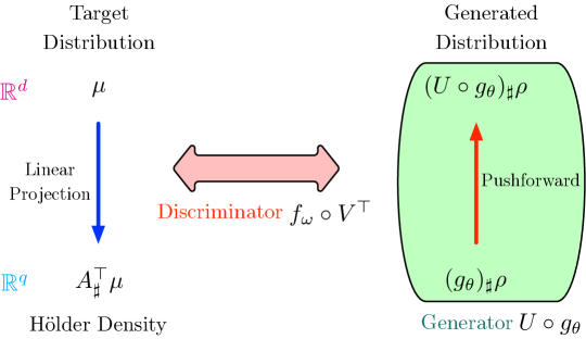
Under Assumption 4, a data point can be represented as , where and is a linear transformation (See graphical illustration in Figure 2). The following lemma formally justifies the existence of the linear transformation .
Lemma 3.
Suppose Assumption 4 holds. Consider a matrix with columns being an orthonormal basis of the -dimensional linear subspace. Then it holds that is a compact and convex subset of , and .
The proof is deferred to Appendix E. The projected domain captures the intrinsic geometric structures in . More importantly, using transformation allows us to define smoothness of the target data distribution. Specifically, we consider a data distribution supported on . Since is a low-dimensional space, does not have a well defined density function with respect to the Lebesgue measure in . Thanks to Lemma 3, the pushforward distribution has a well-defined density function. Accordingly, we make the following data distribution assumption.
Assumption 5.
Without loss of generality, we assume . Given a Hölder index , the density function of belongs to with a bounded Hölder norm for some constant , and on for some constant .
We assume for convenience. Otherwise, we can rescale the input space by a constant , so that the projected space . Since is compact, the constant is bounded and will not undermine the statistical rate of convergence.
To generate samples mimicking data distribution , we consider transforming a -dimensional easy-to-sample distribution supported on to leverage the structural assumption in domain . We define the generator network architecture as
| (12) |
Note that lifts the transformed easy-to-sample distribution to . We expect to extract the linear structures in data, while approximates an optimal transport plan for transforming to .
Pairing with the generator, we define the discriminator network architecture as
| (13) |
The matrix is chosen to “couple” with the linear structures learned by the generator (“anti-projection”) and will approximate Lipschitz functions in for approximating Wasserstein distance. We remark that an appropriate choice of Lipschitz coefficient on will not undermine the approximation power of as confirmed in Lemma 10. Meanwhile, the Lipschitz constraint of discriminator ensures that the generator can accurately capture the linear structures in data. In practice, such a Lipschitz regularity is often enforced by computational heuristics [47, 48, 49].
With proper configurations of network classes (12) and (13), we train GANs using (2) (see Figure 3 for an illustration) and denote the optimizer as , i.e.,
The following theorem establishes a fast statistical rate of convergence of to data distribution .
Theorem 3.
Compared to Theorem 2, we observe that the sizes of generator and discriminator in Theorem 3 crucially depend on and only weakly depend on . Meanwhile, the rate of convergence is fast as the exponent only depends on . This result provides important understandings of why GANs can circumvent the curse of dimensionality in real-world applications, since low-dimensional intrinsic structures are often seen in real-world data sets. Nonetheless, linear structures in Assumption 4 is largely simplified, as it is rare the case that real-world data lie in a subset of a low-dimensional linear subspace (see a generalization to nonlinear mixture data in Section 5). At the same time, real data are often contaminated with observational noise and concentrate only near a low-dimensional manifold.
Theorem 3 demonstrates that GANs with properly chosen generator and discriminator are adaptive to the unknown linear structures in data. Since data are concentrated on a linear subspace, one may advocate PCA-like methods for estimating the linear structure first and then learn the data distribution on a projected subspace. However, such a method requires two-step learning and is rarely used in practical GANs. In fact, GANs simultaneously capture the linear structure and learning the target data distribution via optimizing the empirical risk (2).
A major difficulty in establishing Theorem 3 is proving GANs can capture the unknown linear structures in data. We exploit the optimality of to prove that is small, i.e., the column spaces of and the ground truth matrix match closely. In particular, the mismatch depends on the approximation power of the generator and discriminator (see Lemma 11). Built upon this crucial ingredient, the remaining analysis focuses on tackling the projected Wasserstein distance with respect to the data transformation (see [50, 51] for applications of projected Wasserstein distance in two-sample test). In this way, we circumvent the curse of ambient dimensionality.
5 Distribution estimation in low-dimensional mixture model
Section 4 provides a detailed study of GANs estimating target distributions with unknown linear structures. The obtained estimation guarantee enjoys a fast convergence rate, dependent on the linear subspace dimension. In this section, we generalize to data distributions with nonlinear intrinsic structures and show that GANs maintain the fast statistical estimation guarantee.
We consider target data distribution supported on being a mixture of components.
Assumption 6.
Data distribution takes the decomposition
| (14) |
where is the prior of the corresponding component.
Moreover, each component is a pushforward distribution of the -dimensional uniform distribution on (). In particular, and is -Hölder continuous for some . Moreover, there exists a constant such that for any .
Mixture data are widely seen in practice. For example, MNIST data set is naturally clustered into groups corresponding to different handwritten digits. Images in CIFAR-10 and ImageNet can also be clustered according to labels. Moreover, the intrinsic dimensions of these data sets are all estimated to be much smaller than their ambient dimensions [46]. In our mixture model, we can view the -dimensional coordinates as the low-dimensional intrinsic parameters, and gives rise to a parametrization of data in the -th component.
We can understand the mixture distribution as the marginal distribution of a random vector , whose distribution further depends on a latent random variable . Specifically, let be a categorical random variable with for . Then we define . It can be checked that the marginal distribution of is . More importantly, introducing such a latent variable allows an easy sampling from the mixture distribution; we will choose the generator network based on this intuition.
Note that Assumption 5 is a special case of Assumption 6, when taking . Assumption 6 also suggests a natural partition of domain . Let . Then we have . This shares the same principle as a low-dimensional manifold embedded in , as can be viewed as a local neighborhood on (although is not necessarily a homeomorphism between and ).
We generate samples using a generator by transforming a uniform distribution on unit cube . In particular, we will use the first coordinate to mimic a latent variable and the remaining coordinates are used to generate in each component. We set the generator network architecture as
and establish a mixture distribution approximation theory.
Proposition 1.
Proposition 1 is proved in Appendix A, which draws motivation from Theorem 1. At a coarse level, the generator network is to approximate in each component. Therefore, the network architecture consists of parallel transformations.
We set the discriminator network architecture as
The discriminator network is to approximating -Lipschitz discriminative functions on . We recall training GANs via optimizing (2) and the optimizer is denoted as . The following theorem provides a fast finite-sample distribution estimation guarantee for learning low-dimensional mixture models.
Theorem 4.
The proof is deferred to Appendix A. We discuss implications of Theorem 4.
-
1.
Fast rate. We obtain a fast rate of convergence in estimating the low-dimensional mixture distribution . This result provides a generalization of linear data in Theorem 3, and better explains the empirical success of GANs in practice. We remark that the rate of convergence in Theorem 4 depends on a positive constant . When is sufficiently large, the convergence rate is arbitrarily close to , yet is always marginally slower. Theorem 2 and 3 share the same spirit by providing explicit logarithmic factors in .
-
2.
Relation to Theorem 3. Theorem 3 considers a special case of Assumption 6 and provides a fine-grained analysis. In particular, in addition to a distribution estimation guarantee, Theorem 3 shows that GANs are capable of accurately recover the unknown linear structures in data (Lemma 11). Theorem 4 generalizes Theorem 3 and shows that GANs are capable of capturing nonlinear data intrinsic structures encoded by ’s.
In addition, Theorem 3 indicates a pairing between generator and discriminator networks, in that, they have comparable sizes (exponentially dependent on ) and there is a coupling between the projection and “anti-projection” layers. Theorem 4 is slightly different: The generator is chosen to learn the low-dimensional nonlinear transformation ’s and the discriminator is capable of approximating any -Lipschitz function in . We observe that the size of discriminator in Theorem 4 is exponentially dependent on . In this sense, we view the discriminator in Theorem 4 being overparameterized. This overparameterization, however, does not undermine the fast statistical convergence, largely due to the Lipschitz continuity property of the discriminator.
6 Related work
Distribution approximation using deep generative models. Using generator to accurately approximate the data distribution is of essential importance in understanding the statistical properties of GANs. [15] considered data distribution being exactly realized by an invertible generator, i.e., all the weight matrices and activation functions are invertible. Such an invertibility requires the width of the generator to be the same as input data dimension . Existing literature has shown that such narrow networks lack approximation ability [52, 53]. In fact, to ensure universal approximation for Lebesgue-integrable functions and functions in , the weakest width requirement needs to be and , respectively. Our work, in contrast, allows the generator to be wide and expressive for any data distribution with Hölder densities.
Approximating empirical distribution using neural networks. After the release of an early version of the manuscript, the authors were aware of a concurrent work studying distribution approximation using generative networks. Specifically, [54] established universal approximation abilities of neural network generators for approximating sub-Gaussian data distributions. They proved the existence of a properly chosen generator architecture for achieving an approximation error of data distribution in Wasserstein-1 distance. Our Theorem 1 shares a similar conclusion to [54] for data distributions with Hölder densities. However, the analysis in [54] is very different and relies on memorizing discretized data distribution using neural networks. More recently, [55] showed that GANs can approximate any data distribution (in any dimension) by transforming an absolutely continuous distribution. The idea is to memorize the empirical data distribution using ReLU networks. Nonetheless, the designed generator is not able to generate new samples (different from the training data), which cannot explain the success of GANs in practice.
Statistical properties of GANs. Statistical guarantees of generative models for distribution estimation has been studied in several works. We compare with existing works in Table 1.
| Generator | Discriminator | Distribution | Metric | |
| Generalization error bound | ||||
| [10, 56, 57] | NN | NN | General (Euclidean) | Weak |
| [15, 58, 16] | Invertible NN | NN | Realizable by invertible NN generators (Eulidean and low-d) | Strong |
| [59] | — | pushforward of sub-Gaussian distributions (Eulidean and low-d) | Sinkhorn | |
| [18] | — | Hölder | General (Euclidean and low-d) | Strong |
| Statistical estimation bound | ||||
| [17] | NN | Lipschitz | pushforward of uniform distributions (low-d) | Strong |
| Ours | NN | NN | Having Hölder densities (Euclidean and low-d) | Strong |
Generalization bound of GANs. [10] studied the generalization error of GANs. Lemma 1 in [10] shows that GANs cannot generalize under the Wasserstein distance and the Jensen-Shannon divergence unless the sample size is , where is the generalization gap. Alternatively, they defined a surrogate metric called “neural net distance” , where is the class of discriminator networks. They proved that GANs generalize under the neural net distance, with sample complexity of . This result has two limitations: 1). The sample complexity depends on some unknown parameters of the discriminator network class (e.g., the Lipschitz constant of discriminators with respect to parameters); 2). A small neural net distance does not necessarily imply that two distributions are close [10, Corollary 3.2], which in turn can not answer (Q1) firmly. Our results are explicit in the network architectures, and provide a statistical convergence of GANs under the Wasserstein distance.
Some follow-up works attempted to address the first limitation in [10]. [56] explicitly quantified the Lipschitz constant and the covering number of the discriminator network. They improved the generalization bound in [10] with the technique in [60]. Whereas the bound has an exponential dependence on the depth of the discriminator. [57] proved a tighter generalization bound under spectral normalization applied to the discriminator, where the bound has a polynomial dependence on the size of the discriminator. These generalization theories rely on the assumption that the generator can approximate the data distribution well with respect to the neural net distance, nonetheless, the existence of such a generator is unknown.
[15] tackled the second limitation in [10], and studied the estimation error of GANs under the Wasserstein distance for a special class of distributions implemented by a generator, while the discriminator is designed to guarantee zero bias (or approximation error). Specifically, [15] showed that for certain generator classes, there exist corresponding discriminator classes with a strong discriminative power against the generator. Particular examples include two-layer ReLU network discriminators (half spaces) for distinguishing Gaussian distributions/mixture of Gaussians, and -layer discriminators for -layer invertible generators. In these examples, if the data distribution can be exactly implemented by some generator, then the neural net distance can provably approximate the Wasserstein distance. Consequently, GANs can generalize under the Wasserstein distance. As mentioned earlier, these results require an invertibility assumption on the generator.
Concurrent with [15], [16] studied the estimation error of GANs under the Sobolev IPMs. [16] considered both nonparametric and parametric settings. In the nonparametric setting, the generator and discriminator network architectures are not explicitly chosen, so the bias of the distribution estimation remains unknown. As a result, the bound cannot provide an explicit sample complexity for distribution estimation. Their parametric results are very similar to [15], which requires the same invertibility assumptions and the data distribution needs to be exactly implementable by the generator.
Generative distribution estimation under IPMs. Recently, several works studied distribution estimation under certain discrepancy measures using generative models, when data exhibit low-dimensional structures [59, 17, 18]. The distribution estimation framework is
and the corresponding statistical rate of estimation is free of the curse of data ambient dimensionality. Specifically, in [59], the generative models are assumed to be continuously differentiable up to order . By simultaneously optimize the choice of latent distribution and generative model , they proved that the Sinkhorn divergence between the generated distribution and data distribution converges only depending on data intrinsic dimension. [17] consider data being generated by a ground truth pushfowrad mapping applied to latent samples from a low-dimensional unit cube, which is a special case of in our Assumption 6. Using Lipschitz generator, they proved that the generalization bound in terms of Wassesrstein-1 distance converges only depending on the dimension of the latent space. More recently, [18] established a generalization bound in terms of Hölder IPMs for generative models and the bound converges depending on data intrinsic dimension. Nonetheless, how well the generator can represent the data distribution remains unclear. It is worth mentioning that [61] considered estimating low-dimensional singular distributions using deep generative models. They adopted a likelihood approach, which is different from GANs. All of the aforementioned results rely on training the generative model by minimizing certain discrepancy metric, e.g., Wasserstein-1 distance and Sinkhorn divergence. There is no explicit discriminator network involved, while our analysis considers neural network discriminators and still provides statistical guarantees of GANs in terms of Wasserstein-1 distance.
Density estimation under IPMs. There is also a line of works considering nonparametric density estimation under IPMs [62, 63]. [62] studied the minimax error under Sobolev IPMs. Later, [63] generalized the minimax result to Besov IPMs for estimating distributions with Besov densities. Yet our work is different from these works. Specifically, the distribution estimation framework in [62, 63] is
| (15) |
where is a density function and denotes a class of density estimators, such as the wavelet-thresholding estimator in [63]. Compared to our framework in (2), we consider the push-forward structure in GANs, where the generator is a multidimensional mapping. In contrast, (15) considers density estimators, where is some density function parameterized by a neural network — involving NO generator architecture which transforms the easy-to-sample distribution to the data distribution. Moreover, to evaluate the integral in (15), one needs to exactly know the feature space , and efficiently sample from . Consequently, [62, 63] only apply to . Besides, only estimating the density function requires extensive extra efforts to sample from it, e.g., using Monte Carlo simulation, due to the lack of the push-forward structure. However, our theories are applicable to push-forward GANs, and allow an efficient sampling of generated (fake) data.
7 Proof of statistical theory in Euclidean space
We provide proofs of Theorem 1 and 2. The developed analytical framework will also be adopted for proving Theorem 3 with additional treatments on low-dimensional structures in Section 8.
7.1 Proof of Theorem 1
Theorem 1 is obtained by combining Lemma 1 and 2. Under Assumption 1 - 3, Lemma 1 ensures the existence of a data transformation such that . The remaining step is to choose a proper generator network for approximating .
If the latent space , we can directly apply Lemma 2 for constructing the generator. Otherwise, if , we define a linear scaling function for any , where denotes a vector of ’s. For the data transformation , we rewrite it as so that it suffices to approximate supported on . retains the same Hölder smoothness as , since is invertible and linear. To this end, without loss of generality, we focus on .
Our generator network architecture is constructed in the following way. By denoting with for , we approximate each coordinate mapping using Lemma 2. For a given error , can be approximated by a ReLU network with layers and neurons and weight parameters. Thus, mapping can be approximated by such networks and we denote as . Further, the distribution approximation error is
7.2 Proof of Theorem 2
We prove an oracle inequality for establishing Theorem 2, which decomposes the distribution estimation error into the generator approximation error , the discriminator approximation error , and the statistical error .
Lemma 4.
Let be the Hölder function class defined on with Hölder index . Define . Then it holds
where , and .
Proof of Lemma 4.
We introduce the empirical data distribution as an intermediate term for bounding . Using the triangle inequality, we derive
| (16) |
where step is obtained by rewriting as
Now we bound using a similar triangle inequality trick:
where the last inequality holds by the identity . Substituting the above ingredients into (7.2), we have
The proof is complete. ∎
We next bound each error term separately. and can be controlled by proper choices of the generator and discriminator architectures. can be controlled based on empirical process [64, 65].
Bounding generator approximation error . We answer this question: Given , how can we properly choose to guarantee ? Later, we will pick based on the sample size , and Hölder indexes and .
Lemma 5.
Proof of Lemma 5.
Without loss of generality, we assume . Otherwise, we can rescale the domain to be a subset of . By Monge map (Lemma 1), there exists a mapping such that . Such a mapping is Hölder continuous, i.e., each coordinate mapping for belongs to . We approximate each function using the network architecture identified in Lemma 2. Specifically, given approximation error . There exists a network architecture with no more than layers and neurons and weight parameters, such that with properly chosen weight parameters, yields an approximation of satisfying . Applying this argument times, we form an approximation of . We show satisfies the following IPM bound
Therefore, choosing gives rise to . ∎
Bounding discriminator approximation error . Analogous to the generator, we pre-define an error , and determine the discriminator architecture.
The discriminator is expected to approximate any function . We have the following result.
Lemma 6.
Given any , there exists a ReLU network architecture with
such that, for any discriminative function , if the weight parameters are properly chosen, this network architecture yields a function satisfying .
Proof of Lemma 6.
Using Lemma 2 immediately yields a network architecture for uniformly approximating functions in . Specifically, let the approximation error be . We choose the network architecture consisting of layers and total number of neurons and weight parameters. The maximum width is . Meanwhile, for any function , we have . Threfore, it is enough to choose and . Accordingly, for any , there exists a function given by the network architecture , such that . To this end, we can establish that for any , inequality holds. ∎
Bounding statistical error . The statistical error term is essentially the concentration of empirical data distribution to its population counterpart. Given a symmetric function class , we show scales with the complexity of the function class .
Lemma 7.
For a symmetric function class with for a constant , we have
where denotes the -covering number of with respect to the norm.
Proof of Lemma 7.
The proof utilizes the symmetrization technique and Dudley’s entropy integral, which can be found in empirical process theory [66, 64]. We prove here for completeness. Let be i.i.d. samples from , independent of ’s. By symmetrization, we derive
where ’s are i.i.d. Rademacher random variables, i.e., . The next step is to discretize the function space . Let be a decreasing series of real numbers with . We construct a collection of coverings on under the function norm with accuracy . Denote the -covering number as . For a given , denote the closest element (in the sense) to in the covering as for . We expand as a telescoping sum as
We choose , i.e., the diameter of the class . Then can be arbitrarily picked from . Therefore, the last term since ’s are symmetric. The first term can be bounded by Cauchy-Schwarz inequality:
We now bound each term in the telescoping sum
Observe
By Massart’s lemma [67, Theorem 3.7], we have
Summing up all the terms indexed by , we establish
It suffices to set . Invoking the identity , we derive
By the assumption, we pick and set the -covering with only one element . This yields the desired result
∎
Now we need to find the covering number of Hölder class and that of the discriminator network. Classical result shows that the -covering number of satisfies [68].
On the other hand, the following lemma quantifies the covering number of .
Lemma 8.
The -covering number of satisfies the bound
Proof of Lemma 8.
To construct a covering for , we discretize each weight parameter by a uniform grid with grid size . To simplify the presentation, we omit the bar notation in this proof. Recall we write as . Let with all the weight parameters at most from each other. Denoting the weight matrices in as and , respectively, we bound the difference as
We derive the following bound on :
where is obtained by induction and . The last inequality holds, since . Substituting back into the bound for , we have
where is obtained by induction. We choose satisfying . Then discretizing each parameter uniformly into grids yields a -covering on . There are totally choices of nonzero entries out of weight parameters. Therefore, the covering number is upper bounded by
The proof is complete. ∎
Combining Lemma 7 and the covering numbers, the statistical error can be bounded by
We find that the first infimum in step is attained at . It suffices to take in the second infimum. By omitting constants and polynomial dependence on , we derive
7.3 Proof of Corollary 1
We need an extra concentration argument on the generated fake samples. This is tackled by an alternative oracle inequality (17) shown in below. The rest of the proof utilizes the same argument in Theorem 2.
Proof of Corollary 1.
We show an alternative oracle inequality for finite generated samples as follows. Inequality (7.2) in the proof of Lemma 4 yields
We further expand the first term on the right-hand side above as
By the optimality of , for any , we have
where the last inequality follows the same argument in the proof of Lemma 7. Combining all the inequalities together, we have
| (17) |
Given the proof of Theorem 2, we only need to bound the extra statistical error terms
In fact, Lemma 7 and Lemma 8 together imply
where the first inequality is obtained by taking in Lemma 7, and its covering number is upper bounded by the product of the covering numbers of and . Putting together, the estimation error can be bounded analogously to Theorem 2 as
It suffices to choose and , which yields
In the case of , we have . The proof is complete. ∎
8 Proof of statistical theory in low-dimensional space
The proof idea follows that of Theorem 2, with extra attentions to the exploitation of low-dimensional structures in data. We first slightly modify the oracle inequality in Lemma 4 to decompose the distribution estimation error.
Lemma 9.
Let be the global optimizer of (2). The following error decomposition holds,
| (18) |
Proof of Lemma 9.
We replicate the error decomposition in (7.2) by taking ,
| (19) |
Using the optimality of , we further bound in the last display as
| (20) |
where in , discriminative class follows the same definition in Lemma 4 with .
By Assumption 5 and the optimal transport theory in Lemma 1, we rewrite the data distribution as a pushforward distribution , where is an -Hölder continuous transport plan. Accordingly, we rewrite the empirical data distribution as , with an empirical version of . Applying Lemma 2 and using the same argument in Theorem 1 for approximating , we obtain as a proper approximation. Note that we have chosen in representing for simplicity. Substituting these notations into (8) gives rise to
| (21) |
where inequality holds by instantiating the infimum in (8) to , and inequality follows by the definition of IPM over class. We substitute (8) into (19), which leads to
| (22) |
Two disciminator approximation error terms share a similar formulation, and we can further provide a simplified upper bound on them. Denote as the lipschitz constant of function , and consider the (HARD) term for example.
| (23) |
Applying the same argement to the (EASY) error term yields
| (24) |
Note that we already used the fact that is a subset of . Plugging (8) and (8) into (8) and taking infimum over , we obtain the desired oracle inequality,
The proof is complete. ∎
In the sequel, we bound error terms in (18) respectively. The generator approximation error can be reduced to approximating . By some manipulation on the intrinsic structures of data distribution, we expect that the statistical error scales with the subspace dimension . The main difficulty stems from bounding the discriminator approximation error. A quick comparison to Lemma 4 indicates that the (EASY) error term may be bounded similarly as in Theorem 2. In contrast, the (HARD) error term involves simultaneously approximating the discriminative function projected into the column space of and . In general, such an approximation error is hardly small unless share approximately the same column space. Fortunately, this is indeed the case as shown in Lemma 11 so that the (HARD) error term can be controlled.
Bounding generator approximation error. Suppose that we require the generator approximation error to be bounded by , i.e.,
It suffices to choose a proper generator architecture such that there exists satisfying . To see this, we take and substitute into the generator approximation error,
where the last inequality holds since has orthonormal columns. We can apply Lemma 2 and 5 for choosing proper network configuration of to ensure the existence of . We recall that is a continuous mapping in by Lemma 1. Therefore, the resulting network architecture has the following configuration
| (25) |
We will choose later in the last step of the proof to balance all the error terms.
Bounding discriminator approximation error. We first consider the (EASY) error term. Suppose that we require the (EASY) discriminator approximation error to be bounded by . We check that once is -Lipschitz and has orthonormal columns, then is also -Lipschitz. To see this, for any , we have
By taking in the (EASY) term, it suffices to ensure that can approximate any -Lipschitz function in a compact subset of . Due to the additional -Lipschitz continuity constraint in (13), we need a stronger universal approximation theory of the discriminator. The following lemma shows that ReLU neural networks can accurately approximating -Lipschitz functions in -norm, while the Lipschitz continuity of the network remains independent of the approximation error.
Lemma 10.
For any , there exists a ReLU network architecture , such that for any target -Lipschitz function defined on with , the architecture yields an approximation satisfying . Moreover, the Lipschitz continuity of is bounded by
The configuration of network architecture is
The proof is defered to Appendix B.1. Lemma 10 improves the approximation guarantee in Lemma 2 with the additional Lipschitz continuity characterization, while the newtork size shares the same order of magnitude when specializing Lemma 2 to and . We take with and all the other parameters the same as in Lemma 10. Since the (EASY) error term is invariant with respect to translations on , we can always assume without loss of generality. It then holds
We next bound the (HARD) term. Recall that we need the column spaces of and to be approximately identical for controlling this error. Thanks to the choice of both the generator and discriminator class, we can show that the column spans of and match up to some error.
Lemma 11.
The full proof is deferred to Appendix B.2. We remark that is always lower bounded by a positive constant for any , since its density is positive on the support by Assumption 5. To establish Lemma 11, we leverage the optimality of and the corresponding discriminator network. We show by contraction that if the column spaces of and do not match closely, there exists a discriminator network capable of distinguishing the generated distribution and data distribution.
Given Lemma 11, we are ready to derive an upper bound for the (HARD) discriminator approximation error term.
| (26) |
where is obtained by taking , and inequality is obtained by the triangle inequality
The first term on the right-hand side of (8) can be bounded using the Lipschitz continuity of , i.e.,
A similar argument applies to
The last term in the right-hand side of (8) is the discriminator approximation error, which is bounded by . As a result, the (HARD) error term is upper bounded by
where the last step is obtained by due to .
Bounding statistical error. Similar to the statistical error in Lemma 4, we can bound it via finite-sample concentration. Yet we can pursue a faster convergence rate here by rewriting the data distribution as a pushforward of a low-dimensional distribution.
From Lemma 12, we observe that the statistical error only depends on dimension . To make sense the result, we rewrite the data distribution . In this way, we can translate the concentration of to in into a counterpart in . Recall that is a distribution with a density by Assumption 5. Threfore, we can apply Lemma 7 to complete the proof. See detailed arguments in Appendix B.3.
Balancing approximation error and statistical error. We collect all the error terms in the oracle inequality of Lemma 9 and choose optimal scalings on and . We list all the error upper bounds in the following for a quick reference.
-
1.
Generator approximation error .
-
2.
Statistical error .
-
3.
(EASY) discriminator approximation error .
-
4.
(HARD) discriminator approximation error .
Summing up four error bounds above yields
Substituting the configuration of in Lemma 10 into the last display, we set . By collecting terms, we derive
The corresponding configurations of generator and discriminator is obtained by substituting and in (25) and Lemma 10, respectively.
9 Conclusion and discussion
We establish statistical convergence of distribution estimation using GANs. Specifically, with proper generator and discriminator network architecture, we show GANs are consistent estimator of data distribution in terms of the Wasserstein distance. Moreover, when data have intrinsic low-dimensional linear structures, we show GANs can capture the unknown linear structure and enjoy a faster statistical rate of estimation, which is free of the curse of dimensionality. Compared to existing works, our theory exploits the pushforward structure of GANs and network architectures are explicitly given without invertibility constraints.
In the sequel, we discuss several related topics and future directions.
Distribution estimation on manifold. Low-dimensional manifolds are sensible tools to model data geometric structures. A manifold can be characterized by local neighborhoods (charts), which generalizes the mixture model in Section 5. Our analysis does not cover manifold data due to the difficulty to accurately approximate target distributions using generator networks. Specifically, different from the mixture model with a pre-fixed partition of components, we often don’t have specific information on how to properly construct charts on the manifold. It is rare the case that an artificially constructed collection of charts can preserve the regularity of target data distributions. This makes choosing a proper generator network difficult.
Convolutional filters and residual connections. Convolutional filters [69] are widely used in GANs for image generating and processing. Empirical results show that convolutional filters can learn hidden representations aligned with various patterns in images [70, 71], e.g., textures and skeletons. An interesting question is to understand how convolutional filters capture the aforementioned low-dimensional structures in data sets.
Smoothness of data distributions and regularized distribution Estimation. Theorem 2 indicates a convergence rate independent of the smoothness of the data distribution. The reason behind is that the empirical data distribution cannot inherit the same smoothness as the underlying data distribution. This limitation exists in all previous works [58, 62, 63]. It is interesting to investigate whether GANs can achieve a faster convergence rate (e.g., attain the minimax optimal rate).
From a theoretical perspective, [16] suggested first obtaining a smooth kernel estimator from , and then replacing by to train GANs. In practice, kernel smoothing is hardly used in GANs. Instead, regularization (e.g., entropy regularization) and normalization (e.g., spectral normalization and batch-normalization) are widely applied as implicit regularizers to promote the smoothness of the learned distribution. Several empirical studies of GANs suggest that divergence-based and mutual information-based regularization can stabilize the training and improve the performance [72, 73] of GANs. We leave the studies on statistical properties of regularized GANs for future investigation.
Computational concerns. Our statistical guarantees hold for the global optimizer of (2), whereas solving (2) is often difficult. In practice, it is observed that larger neural networks are easier to train and yield better statistical performance [74, 75, 76, 77, 78, 79, 80, 81, 82]. This is referred to as overparameterization. Establishing a connection between computation and statistical properties of GANs is an important direction.
References
- [1] I. Goodfellow, J. Pouget-Abadie, M. Mirza, B. Xu, D. Warde-Farley, S. Ozair, A. Courville, and Y. Bengio, “Generative adversarial nets,” in Advances in neural information processing systems, pp. 2672–2680, 2014.
- [2] S. Reed, Z. Akata, X. Yan, L. Logeswaran, B. Schiele, and H. Lee, “Generative adversarial text to image synthesis,” arXiv preprint arXiv:1605.05396, 2016.
- [3] C. Ledig, L. Theis, F. Huszár, J. Caballero, A. Cunningham, A. Acosta, A. Aitken, A. Tejani, J. Totz, Z. Wang, et al., “Photo-realistic single image super-resolution using a generative adversarial network,” in Proceedings of the IEEE conference on computer vision and pattern recognition, pp. 4681–4690, 2017.
- [4] K. Schawinski, C. Zhang, H. Zhang, L. Fowler, and G. K. Santhanam, “Generative adversarial networks recover features in astrophysical images of galaxies beyond the deconvolution limit,” Monthly Notices of the Royal Astronomical Society: Letters, vol. 467, no. 1, pp. L110–L114, 2017.
- [5] A. Brock, J. Donahue, and K. Simonyan, “Large scale gan training for high fidelity natural image synthesis,” arXiv preprint arXiv:1809.11096, 2018.
- [6] V. Volz, J. Schrum, J. Liu, S. M. Lucas, A. Smith, and S. Risi, “Evolving mario levels in the latent space of a deep convolutional generative adversarial network,” in Proceedings of the Genetic and Evolutionary Computation Conference, pp. 221–228, 2018.
- [7] A. Radford, L. Metz, and S. Chintala, “Unsupervised representation learning with deep convolutional generative adversarial networks,” arXiv preprint arXiv:1511.06434, 2015.
- [8] T. Salimans, I. Goodfellow, W. Zaremba, V. Cheung, A. Radford, and X. Chen, “Improved techniques for training gans,” in Advances in neural information processing systems, pp. 2234–2242, 2016.
- [9] A. Müller, “Integral probability metrics and their generating classes of functions,” Advances in Applied Probability, vol. 29, no. 2, pp. 429–443, 1997.
- [10] S. Arora, R. Ge, Y. Liang, T. Ma, and Y. Zhang, “Generalization and equilibrium in generative adversarial nets (gans),” arXiv preprint arXiv:1703.00573, 2017.
- [11] V. Nair and G. E. Hinton, “Rectified linear units improve restricted boltzmann machines,” in Proceedings of the 27th international conference on machine learning (ICML-10), pp. 807–814, 2010.
- [12] X. Glorot, A. Bordes, and Y. Bengio, “Deep sparse rectifier neural networks,” in Proceedings of the fourteenth international conference on artificial intelligence and statistics, pp. 315–323, 2011.
- [13] A. L. Maas, A. Y. Hannun, and A. Y. Ng, “Rectifier nonlinearities improve neural network acoustic models,” in ICML Workshop on Deep Learning for Audio, Speech, and Language Processing, 2013.
- [14] I. Goodfellow, Y. Bengio, and A. Courville, Deep Learning. Cambridge, MA, USA: MIT Press, 2016.
- [15] Y. Bai, T. Ma, and A. Risteski, “Approximability of discriminators implies diversity in gans,” arXiv preprint arXiv:1806.10586, 2018.
- [16] T. Liang, “On how well generative adversarial networks learn densities: Nonparametric and parametric results,” arXiv preprint arXiv:1811.03179, 2018.
- [17] N. Schreuder, V.-E. Brunel, and A. Dalalyan, “Statistical guarantees for generative models without domination,” in Algorithmic Learning Theory, pp. 1051–1071, PMLR, 2021.
- [18] A. Block, Z. Jia, Y. Polyanskiy, and A. Rakhlin, “Intrinsic dimension estimation,” arXiv preprint arXiv:2106.04018, 2021.
- [19] C. Villani, Optimal transport: old and new, vol. 338. New York, NY, USA: Springer Science & Business Media, 2008.
- [20] T.-W. Lee and M. S. Lewicki, “Unsupervised image classification, segmentation, and enhancement using ica mixture models,” IEEE Transactions on Image Processing, vol. 11, no. 3, pp. 270–279, 2002.
- [21] N. Chen, J. Zhu, and E. Xing, “Predictive subspace learning for multi-view data: a large margin approach,” Advances in neural information processing systems, vol. 23, 2010.
- [22] X. Fang, S. Teng, Z. Lai, Z. He, S. Xie, and W. K. Wong, “Robust latent subspace learning for image classification,” IEEE transactions on neural networks and learning systems, vol. 29, no. 6, pp. 2502–2515, 2017.
- [23] M. Caron, P. Bojanowski, A. Joulin, and M. Douze, “Deep clustering for unsupervised learning of visual features,” in Proceedings of the European conference on computer vision (ECCV), pp. 132–149, 2018.
- [24] F. Santambrogio, “Models and applications of optimal transport in economics, traffic and urban planning,” arXiv preprint arXiv:1009.3857, 2010.
- [25] A. Galichon, “A survey of some recent applications of optimal transport methods to econometrics,” 2017.
- [26] Y. Ganin and V. Lempitsky, “Unsupervised domain adaptation by backpropagation,” arXiv preprint arXiv:1409.7495, 2014.
- [27] N. Courty, R. Flamary, D. Tuia, and A. Rakotomamonjy, “Optimal transport for domain adaptation,” IEEE transactions on pattern analysis and machine intelligence, vol. 39, no. 9, pp. 1853–1865, 2016.
- [28] G. Monge, Mémoire sur le calcul intégral des équations aux différences partielles. Paris, France: Imprimerie royale, 1784.
- [29] L. A. Caffarelli, “The regularity of mappings with a convex potential,” Journal of the American Mathematical Society, vol. 5, no. 1, pp. 99–104, 1992.
- [30] L. A. Caffarelli, “Boundary regularity of maps with convex potentials,” Communications on pure and applied mathematics, vol. 45, no. 9, pp. 1141–1151, 1992.
- [31] L. A. Caffarelli, “Boundary regularity of maps with convex potentials–ii,” Annals of mathematics, pp. 453–496, 1996.
- [32] J. I. Urbas, “Regularity of generalized solutions of monge-ampere equations,” Mathematische Zeitschrift, vol. 197, no. 3, pp. 365–393, 1988.
- [33] J. Urbas, “On the second boundary value problem for equations of monge-ampere type,” Journal fur die Reine und Angewandte Mathematik, vol. 487, pp. 115–124, 1997.
- [34] G. Cybenko, “Approximation by superpositions of a sigmoidal function,” Mathematics of control, signals and systems, vol. 2, no. 4, pp. 303–314, 1989.
- [35] K. Hornik, “Approximation capabilities of multilayer feedforward networks,” Neural networks, vol. 4, no. 2, pp. 251–257, 1991.
- [36] C. K. Chui and X. Li, “Approximation by ridge functions and neural networks with one hidden layer,” Journal of Approximation Theory, vol. 70, no. 2, pp. 131–141, 1992.
- [37] A. R. Barron, “Universal approximation bounds for superpositions of a sigmoidal function,” IEEE Transactions on Information theory, vol. 39, no. 3, pp. 930–945, 1993.
- [38] H. N. Mhaskar, “Neural networks for optimal approximation of smooth and analytic functions,” Neural computation, vol. 8, no. 1, pp. 164–177, 1996.
- [39] D. Yarotsky, “Error bounds for approximations with deep relu networks,” Neural Networks, vol. 94, pp. 103–114, 2017.
- [40] L. Wasserman, All of nonparametric statistics. New York, NY, USA: Springer Science & Business Media, 2006.
- [41] A. B. Tsybakov, Introduction to nonparametric estimation. New York, NY, USA: Springer Science & Business Media, 2008.
- [42] J. Moser, “On the volume elements on a manifold,” Transactions of the American Mathematical Society, vol. 120, no. 2, pp. 286–294, 1965.
- [43] R. Tang and Y. Yang, “Minimax rate of distribution estimation on unknown submanifold under adversarial losses,” arXiv preprint arXiv:2202.09030, 2022.
- [44] J. B. Tenenbaum, V. De Silva, and J. C. Langford, “A global geometric framework for nonlinear dimensionality reduction,” Science, vol. 290, no. 5500, pp. 2319–2323, 2000.
- [45] S. T. Roweis and L. K. Saul, “Nonlinear dimensionality reduction by locally linear embedding,” science, vol. 290, no. 5500, pp. 2323–2326, 2000.
- [46] P. Pope, C. Zhu, A. Abdelkader, M. Goldblum, and T. Goldstein, “The intrinsic dimension of images and its impact on learning,” arXiv preprint arXiv:2104.08894, 2021.
- [47] A. Virmaux and K. Scaman, “Lipschitz regularity of deep neural networks: analysis and efficient estimation,” Advances in Neural Information Processing Systems, vol. 31, 2018.
- [48] P. Pauli, A. Koch, J. Berberich, P. Kohler, and F. Allgöwer, “Training robust neural networks using lipschitz bounds,” IEEE Control Systems Letters, vol. 6, pp. 121–126, 2021.
- [49] H. Gouk, E. Frank, B. Pfahringer, and M. J. Cree, “Regularisation of neural networks by enforcing lipschitz continuity,” Machine Learning, vol. 110, no. 2, pp. 393–416, 2021.
- [50] J. Wang, R. Gao, and Y. Xie, “Two-sample test using projected wasserstein distance: Breaking the curse of dimensionality,” arXiv preprint arXiv:2010.11970, 2020.
- [51] J. Wang, M. Chen, T. Zhao, W. Liao, and Y. Xie, “A manifold two-sample test study: Integral probability metric with neural networks,” arXiv preprint arXiv:2205.02043, 2022.
- [52] Z. Lu, H. Pu, F. Wang, Z. Hu, and L. Wang, “The expressive power of neural networks: A view from the width,” in Advances in neural information processing systems, pp. 6231–6239, 2017.
- [53] S. Park, C. Yun, J. Lee, and J. Shin, “Minimum width for universal approximation,” arXiv preprint arXiv:2006.08859, 2020.
- [54] Y. Lu and J. Lu, “A universal approximation theorem of deep neural networks for expressing probability distributions,” Advances in neural information processing systems, vol. 33, pp. 3094–3105, 2020.
- [55] J. Huang, Y. Jiao, Z. Li, S. Liu, Y. Wang, and Y. Yang, “An error analysis of generative adversarial networks for learning distributions,” Journal of Machine Learning Research, vol. 23, no. 116, pp. 1–43, 2022.
- [56] P. Zhang, Q. Liu, D. Zhou, T. Xu, and X. He, “On the discrimination-generalization tradeoff in gans,” arXiv preprint arXiv:1711.02771, 2017.
- [57] H. Jiang, Z. Chen, M. Chen, F. Liu, D. Wang, and T. Zhao, “On computation and generalization of gans with spectrum control,” arXiv preprint arXiv:1812.10912, 2018.
- [58] T. Liang, “How well can generative adversarial networks learn densities: A nonparametric view,” arXiv preprint arXiv:1712.08244, 2017.
- [59] G. Luise, M. Pontil, and C. Ciliberto, “Generalization properties of optimal transport gans with latent distribution learning,” arXiv preprint arXiv:2007.14641, 2020.
- [60] P. L. Bartlett, D. J. Foster, and M. J. Telgarsky, “Spectrally-normalized margin bounds for neural networks,” in Advances in Neural Information Processing Systems, pp. 6240–6249, 2017.
- [61] M. Chae, D. Kim, Y. Kim, and L. Lin, “A likelihood approach to nonparametric estimation of a singular distribution using deep generative models,” arXiv preprint arXiv:2105.04046, 2021.
- [62] S. Singh, A. Uppal, B. Li, C.-L. Li, M. Zaheer, and B. Póczos, “Nonparametric density estimation under adversarial losses,” in Advances in Neural Information Processing Systems, pp. 10225–10236, 2018.
- [63] A. Uppal, S. Singh, and B. Póczos, “Nonparametric density estimation & convergence of gans under besov ipm losses,” arXiv preprint arXiv:1902.03511, 2019.
- [64] A. W. Van Der Vaart and J. A. Wellner, “Weak convergence,” in Weak convergence and empirical processes, pp. 16–28, New York, NY, USA: Springer, 1996.
- [65] L. Györfi, M. Kohler, A. Krzyzak, and H. Walk, A distribution-free theory of nonparametric regression. New York, NY, USA: Springer Science & Business Media, 2006.
- [66] R. M. Dudley, “The sizes of compact subsets of hilbert space and continuity of gaussian processes,” Journal of Functional Analysis, vol. 1, no. 3, pp. 290–330, 1967.
- [67] M. Mohri, A. Rostamizadeh, and A. Talwalkar, Foundations of machine learning. Cambridge, MA, USA: MIT press, 2018.
- [68] R. Nickl and B. M. Pötscher, “Bracketing metric entropy rates and empirical central limit theorems for function classes of besov-and sobolev-type,” Journal of Theoretical Probability, vol. 20, no. 2, pp. 177–199, 2007.
- [69] A. Krizhevsky, I. Sutskever, and G. E. Hinton, “Imagenet classification with deep convolutional neural networks,” in Advances in neural information processing systems, pp. 1097–1105, 2012.
- [70] M. D. Zeiler and R. Fergus, “Visualizing and understanding convolutional networks,” in European conference on computer vision, pp. 818–833, Springer, 2014.
- [71] B. Zhou, D. Bau, A. Oliva, and A. Torralba, “Interpreting deep visual representations via network dissection,” IEEE transactions on pattern analysis and machine intelligence, vol. 41, no. 9, pp. 2131–2145, 2018.
- [72] T. Che, Y. Li, A. P. Jacob, Y. Bengio, and W. Li, “Mode regularized generative adversarial networks,” arXiv preprint arXiv:1612.02136, 2016.
- [73] Y. Cao, G. W. Ding, K. Y.-C. Lui, and R. Huang, “Improving gan training via binarized representation entropy (bre) regularization,” arXiv preprint arXiv:1805.03644, 2018.
- [74] C. Zhang, S. Bengio, M. Hardt, B. Recht, and O. Vinyals, “Understanding deep learning requires rethinking generalization,” arXiv preprint arXiv:1611.03530, 2016.
- [75] A. Jacot, F. Gabriel, and C. Hongler, “Neural tangent kernel: Convergence and generalization in neural networks,” in Advances in neural information processing systems, pp. 8571–8580, 2018.
- [76] S. S. Du, J. D. Lee, H. Li, L. Wang, and X. Zhai, “Gradient descent finds global minima of deep neural networks,” arXiv preprint arXiv:1811.03804, 2018.
- [77] Z. Allen-Zhu, Y. Li, and Z. Song, “A convergence theory for deep learning via over-parameterization,” arXiv preprint arXiv:1811.03962, 2018.
- [78] S. S. Du, X. Zhai, B. Poczos, and A. Singh, “Gradient descent provably optimizes over-parameterized neural networks,” arXiv preprint arXiv:1810.02054, 2018.
- [79] Y. Li and Y. Liang, “Learning overparameterized neural networks via stochastic gradient descent on structured data,” in Advances in Neural Information Processing Systems, pp. 8157–8166, 2018.
- [80] S. Arora, S. S. Du, W. Hu, Z. Li, and R. Wang, “Fine-grained analysis of optimization and generalization for overparameterized two-layer neural networks,” arXiv preprint arXiv:1901.08584, 2019.
- [81] Z. Allen-Zhu, Y. Li, and Y. Liang, “Learning and generalization in overparameterized neural networks, going beyond two layers,” in Advances in neural information processing systems, pp. 6155–6166, 2019.
- [82] S. S. Du and W. Hu, “Width provably matters in optimization for deep linear neural networks,” arXiv preprint arXiv:1901.08572, 2019.
- [83] M. Chen, H. Jiang, W. Liao, and T. Zhao, “Efficient approximation of deep relu networks for functions on low dimensional manifolds,” in Advances in Neural Information Processing Systems, pp. 8172–8182, 2019.
- [84] J. Weed and F. Bach, “Sharp asymptotic and finite-sample rates of convergence of empirical measures in wasserstein distance,” Bernoulli, vol. 25, no. 4A, pp. 2620–2648, 2019.
- [85] M. J. Wainwright, High-dimensional statistics: A non-asymptotic viewpoint, vol. 48. Cambridge University Press, 2019.
Appendix A Proof of Theorem 4
The proof is built upon the framework for establishing Theorem 2. We restate the oracle inequality in Lemma 4 (with ):
The remaining proof consists of two major parts: 1) bounding generator approximation error ; 2) fast convergence of . Note that the discriminator approximation error is a direct consequence of Lemma 10 (replacing by ).
Bounding generator approximation error. Given , we constructively show the existence of a generator network architecture giving rise to an approximation of .
Lemma 13 (Restatement of Proposition 1).
Suppose Assumption 6 holds. Given any , we choose network architecture with
Then there exists such that
Proof of Lemma 13.
We adopt a two-step construction: 1) we use the first coordinate of to generate a latent variable approximately distributed like for ; 2) we use the remaining coordinates of to generate data approximating each component in the mixture.
Generating latent variable. Let for and . We define a trapezoid function on as
See Figure 4 for an illustration.

Passing the first coordinate through yields an approximate binary random variable, with and .
Generating each component. Since each component can be represented by , it suffices to approximate using neural networks. Given the regularity of in Assumption 6, invoking Theorem 1 (built upon Lemma 2), we obtain that there exists a neural network that yields an approximation of with
Such a network has
| (27) |
Putting together. For any , we obtain a generated sample by
| (28) |
where . However, (28) cannot be exactly implemented by a neural network due to the multiplication operation. We adopt Proposition 3 in [39] (see also Corollary 1 in [83]) for approximating multiplication. Specifically, we denote as an -approximation of multiplication and applying it entrywise yields
We use an abstract notation to denote the mapping from to . Now we bound the distribution approximation error
Term is bounded by since is an -approximation of multiplication. Term can be estimated as follows.
Adding and , we obtain
The remaining step is to determine the network size for implementing . Note that can be exactly represented by a network. In particular, consists of parallel sub-networks, each computing . By Corollary 1 in [83], can be implemented by a -depth constant-width network. is a piecewise linear function with at most break points. Thus can be realized by a single-layer constant-width network. We remark that using a single layer network for implementing requires the weight parameter to be as large as . In order to have constant bounded weight parameters, we utilize the same trick in the proof of Lemma 10 (Appendix B.1). As a consequence, we need a -depth constant-width for realizing . Lastly, the network size for is given in (27). Putting together, we have implementable by with
| (29) |
Proposition 1 holds by observing for any . ∎
Bounding statistical error. Given , Lemma 10 suggests that we can choose with
| (30) |
such that any -Lipschitz function on can be approximated by up to error . Since functions in is -Lipschitz continuous, we have
We invoke the following fast convergence of empirical data distribution to its population counterpart in terms of Wasserstein-1 distance.
Lemma 14 (Theorem 1 in [84]).
For any , we have
where is the upper Wasserstein dimension of distribution (Definition 4 in [84]) and is independent of .
To apply Lemma 14, we need to find under Assumption 6. It suffices to upper bound using
| (31) |
where is the covering number of . We construct a covering of utilizing ’s to bound the covering number. For , let be an -covering of . We claim that forms an -covering of . To see this, let be arbitrary. There exists at least one , such that for some . We can find satisfying . Then we evaluate
Equality follows from first-order Taylor expansion. Inequality follows from . The covering number of a unit cube can be obtained by a volume ratio argument [85, Lemma 5.2],
Using the last display, the cardinality of is bounded by . Substituting into (31), we have
Consequently, the statistical error is bounded by
Balancing error terms. Summing up generator/discriminator approximation error and statistical error in the oracle inequality, we derive
It suffices to choose , which gives rise to
where is independent of . Substituting into the generator and discriminator sizes in (29) and (30), respectively, we complete the proof.
Appendix B Detailed proofs in Section 8
B.1 Proof of Lemma 10
Proof of Lemma 10.
The proof consists of two steps: 1) construction of a piecewise linear function for approximating -Lipschitz functions, which can be implemented by a ReLU neural network; 2) establishing the global Lipschitz continuity of the neural network, in addition to the approximation error guarantee.
Step 1). Given a positive integer , we evenly choose points in the hypercube , denoted as with . We define a univariate trapezoid function (see graphical illustration in Figure 5)
Then for any , we define a partition of unity based on a product of trapezoid functions indexed by ,

For any target -Lipschitz function , it is more convenient to write its Lipschitz continuity with respect to the norm, i.e.,
| (32) |
We now define a collection of piecewise constant functions
We claim that is an approximation of , with an approximation error evaluated as
where the last inequality follows from the Lipschitz continuity in (32) and the fact that there are at most terms in the summation.
We use a ReLU network to implement . It turns out that we only need to implement the multiplication operation in . For scalars , we rewrite as . We know neural networks can approximate a univariate quadratic function on as
| (33) |
where . The approximation error of is (A proof can be found in [39, Proposition 2] or [83, Lemma 1]). We approximate recursively using univariate quadratic functions. Specifically, we construct
| (34) |
where for . Then the network for approximating is obtained as
| (35) |
We bound approximation error of as
where the last inequality follows from recursively decomposing into terms as
and observing
for any .
Step 2). The following lemma establishes the Lipschitz continuity of with respect to the norm.
Lemma 15.
Let be defined in (35). Then for any , it holds
The proof is deferred to Appendix C. Given Lemma 15, we choose and satisfying
which implies . As a result, we check the approximation error of as
Meanwhile, with the choice of and , Lemma 15 implies that for any , it holds
The remaining step is to characterize the size of the ReLU network for implementing . Construction (35) suggests that the network consists of parallel subnetworks. In each subnetwork, we need to implement defined in (34), where the subnetwork architecture consists of layers and the width is bounded by a constant (since is realizable by a width- network). Putting together all the parallel subnetworks, we conclude that the whole network architecture consists of layers and the width is bounded by . Substituting our choice of and into the network size, we obtain and . The total number of neurons and nonzero weight parameters in the network is .
The last step is to ensure that each weight parameter in is bounded by a constant. The only caveat stems from the trapezoid function in , which is rescaled by (see equation (34)). We use a deep network to implement . Consider a basic step function , whose -th order composition is
Setting , we observe that has a slope of at least . We use to realize the left linear segment in . For the right linear segment, we can use instead. In this way, we increment the network architecture for implementing by a depth of and a width of , while each weight parameter in the network is bounded by a constant. To summarize the network architecture, we have
The bound on is obtained by combining Lipschitz continuity (32) with .
∎
B.2 Proof of Lemma 11
Proof of Lemma 11.
Given the choice of generator and discriminator network classes, we show that at a global optimizer , it holds
| (36) |
Suppose for the purpose of contradiction, we have
| (37) |
We will prove that there exists such that
| (38) |
On the other hand, by choosing and with , we have
| (39) |
since discriminator is -Lipschitz with respect to the norm. Putting (B.2) and (39) together, we conclude that cannot be a global optimizer. Therefore, (B.2) holds true. It remains to establish (B.2). Since the discriminator network can approximate any -Lipschitz function by Lemma 10, it is convenient to show the following sufficient condition for (B.2),
| (40) |
In fact, (40) implies that for any , there exists a discriminative function and matrix such that . By choosing as an -approximation of and , we obtain
which establishes (B.2).
To ease the presentation, we recall that . We now consider two complementary cases for establishing (40),
-
•
(Case 1) ;
-
•
(Case 2) ,
where denotes the -th coordinate mapping. Note that (Case 2) says that the column spaces of are nearly identical. We tackle the two cases separately. To further ease the analysis, we assume without loss of generality that for , where and are column vectors of and , respectively. Otherwise we can replace with and with simultaneously. As a result, we may remove the absolute values in (Case 1) and (Case 2) for simplicity.
(Case 1) We show that there exists an index such that the corresponding column vectors and are sufficiently mis-aligned in direction. Specifically, given , we expand the expression as
Since for , by the Pigeonhole principle, we deduce that there exists an index with
| (41) |
Now we prove that the mis-alignment of and already results in a sufficient separation between the generated distribution and data distribution, in terms of projected Wasserstein distance. By definition, we have
| (42) |
We choose the projection matrix to be a rank- matrix with only the -th column nonzero, i.e.,
We further choose a specific testing function to derive a lower bound on (42). Let be linear with and for . Substituting our choice of and into (42), we obtain
| (43) |
Using (41), we lower bound
Substituting into (43), we conclude
(Case 2) The assertion of (Case 2) translates to several useful spectral norm bounds. We first observe
| (44) |
Taking square root on both sides of (B.2), we have . In addition, since has orthonormal columns, we have
| (45) |
We use a similar proof strategy as in (Case 1) by choosing a specific projection matrix , and evaluate the Wasserstein distance
| (46) |
Invoking inequality (B.2), assumes the upper bound
To lower bound , we prove a lower bound on . The triangle inequality implies
We bound the second term in the right-hand side above as
where inequality invokes the Lipschitz continuity of and inequality invokes (B.2). Recall that in (B.2), we assume
Thus, we have
which implies
Combining the bounds of and and substituting into (46), we obtain
which checks (Case 2). Putting (Case 1) and (Case 2) together, we establish inequality (40). Consequently, (B.2) holds true and therefore, (B.2) is valid for a global optimizer .
Next, we show given (B.2), the column space of and are approximately equal. In particular, we show the following bound
Suppose not. We expand the squared Frobenius norm as
From the last display above, we deduce
We consider distinguish and by a linear testing function , where the index verifies
Repeating the same argument in (Case 1), we deduce
which contradicts (39). The proof is complete. ∎
B.3 Proof of Lemma 12
Proof of Lemma 12.
We bound first. Denote and . By Assumption 4, we write as
| (47) |
where in , the composite function is Lipschitz continuous, whose Lipschitz constant is bounded by . Applying Lemma 7, with the function class being -Lipschitz functions on , we derive
| (48) |
where in , we substitute a covering number bound , and in , we take and distinguish two cases depending on :
-
•
(). Inequality can be simplified as
-
•
(). Inequality can be computed as
Applying Lemma 7 again, with the function class being , we further have
| (49) |
where in , we invoke Lemma 8 instantiated to , and in , we set .
∎
Appendix C Proof of Lemma 15
Proof of Lemma 15.
We begin by considering two points differing in only one coordinate. Without loss of generality, we assume , while for . We have two base cases:
-
•
(Base case 1) there exists such that ;
-
•
(Base case 2) there exists such that .
In both base cases, and are close enough within distance . Later, we will reduce general positions of to a collection of base bases. A graphical illustration of base cases are given in Figure 6.

In (Base case 1), we have and for any . Therefore, the equality holds true for any . Consequently, we deduce .
In (Base case 2), the analysis is more complicated. We first observe that and are both nonzero, while for any (the same holds for ). Denote as all the entries in except the first entry . We rewrite as
The second equality above holds, since whenever . Furthermore, we have
| (50) |
In order to bound the right-hand side of (C), we establish several regularity properties of based on Lemma 18. The first result proves the monotonicity of .
Lemma 16.
Let be defined in (34). Consider two points and only differing in the -th coordinate. Denote satisfying . Then it holds
The proof is deferred to Appendix C.1.2. Next, we show first-order continuity of .
Lemma 17.
Let be defined in (34). Consider two points and only differing in the -th coordinate. Then for any , it holds
The proof is deferred to Appendix C.1.3. Using Lemma 16 and 17, we are able to bound the right-hand side of (C). We partition all the values of into two complementary disjoint sets:
In , by the Lipschitz continuity of , we have
If either or , then and should be both positive or negative. Their product must be positive. As a result, we deduce that in ,
hold simultaneously.
In , and are both positive or negative. We rewrite (C) according to the partition of and on :
| (51) |
where
For term , we bound it by
| (52) |
where inequality invokes Lemma 17 and neglects terms involving and inequality expands the product by noting . To see inequality , we first observe that there are at most terms in the summation, due to the definition of . Then we bound as
Meanwhile, is indeed a partition of unity on a -dimensional unit cude. Therefore, we have
For term , we leverage the cancellation in the two summations. We assume without loss of generality, and for . Otherwise, replacing by won’t change term . Therefore, we derive
| (53) |
where inequality uses the monotonicity of in Lemma 16, inequality invokes Lemma 17, and inequality follows from the same argument of in (C). Combining (C), (C) and substituting into (51), we obtain
| (54) |
Given two base cases, we proceed to show Lipschitz continuity of . We first partition into two types of sub-intervals,
(Type 1) and (Type 2) ,
where is an integer. We observe that on a (Type 1) sub-interval, (Base case 1) applies; while on a (Type 2) sub-interval, (Base case 2) applies. Depending on the location of and , we discuss four situations.
(Situation 1): belongs to a (Type 1) sub-interval and belongs to a (Type 1) sub-interval. If the two sub-intervals coincide, we obtain (Base case 1). There is nothing to show. Otherwise, we denote integer such that and integer such that . See Figure 7 for an illustration.
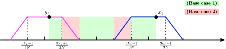
We can derive
where inequality follows from (Base case 1). If , then we can apply (Base case 2) to show
Otherwise, we have
where inequality is obtained by applying (Base case 2) twice. To complete the argument, we can replace and and repeat the derivation to accumulate all the differences yielded on a (Type 2) sub-interval, until or for some integer . Consequently, noting that the total length of (Type 2) interval between and is always smaller than , we deduce
(Situation 2): belongs to a (Type 1) sub-interval and belongs to a (Type 2) sub-interval. We aim to reduce this situation to (Situation 1). Following the same notation, we denote for some integer and for . Triangle inequality yields
We now observe that term falls into (Situation 1). A straightforward adaptation of the argument in (Situation 1) gives rise to
(Situation 3): belongs to a (Type 2) sub-interval and belongs to a (Type 1) sub-interval. The analysis is analogous to (Situation 2) by switching and . Denoting for some integer and for , we derive
Note that falls into (Situation 1). Therefore, the desired Lipschitz continuity (54) holds.
(Situation 4): belongs to a (Type 2) sub-interval and belongs to a (Type 2) sub-interval. If the two sub-intervals coincide, this recovers (Base case 2), and there is nothing to show. Otherwise, applying the analysis in (Situation 2) and (Situation 3) consecutively to move first into a (Type 1) sub-interval and then , we reduce this situation to (Situation 1) again. Therefore, Lipschitz continuity in (54) still holds true.
Combining all four situations, for any only differing in the first coordinate, it holds
The proof is complete for general by aggregating coordinate-wise differences and the fact . ∎
C.1 Proofs of supporting results for Lemma 15
Before we present omitted proofs in Lemma 15, we study the regularity of the approximated square function , which will be frequently used in proving Lemma 16 and Lemma 17.
C.1.1 Regularity of
Given a function , for any , we define upper and lower slopes at , denoted by and , respectively, as
The definition above coincides with upper and lower derivatives of a univariate function. We use “slope” instead of derivatives as we will instantiate the definition to the piecewise linear function . We show several useful properties.
Lemma 18.
For a given positive integer , let be defined on as in (33). Then the following identities hold.
-
1.
For any , we have
(55) (56) -
2.
Given an integer , we denote as the -bit binary encoding of , that is, . Then for any , we have
(57) (58)
Proof of Lemma 18.
By construction, is a piecewise linear function. Each of its linear segment is supported on a sub-interval for . Therefore, it can be checked that is also a piecewise linear function, since it is a linear combination of ’s. Furthermore, the -th linear segment in has a slope , i.e., on open interval . As a result, is differentiable on and its derivative satisfies
| (59) |
We observe for , which implies . For any , we have
Thus, we deduce and (C.1.1) can be simplified as
| (60) |
We claim
| (61) |
where is the -th entry of the -bit binary encoding . In other words, the parity of is encoded by . In particular, if is odd (resp. even), (resp. ).
To show the claim in (61), we first prove
for any . Indeed, we can show the following sandwich inequality
| (62) |
Inequality holds, since ; inequality holds, since . Substituting into (62), we derive
Due to , we conclude . Consequently, we deduce , which verifies the claim by noting .
To establish the first assertion in Lemma 18, we only need to consider end points of each linear segment of . Otherwise, when for some , (63) shows is differentiable at , and therefore, (55) holds true. Consider an end point for some . We evaluate left and right derivatives of at . We denote left and right derivatives as and , respectively. Using (63) again, we derive
We note , and therefore, for , we obtain
| (64) | ||||
This establishes the first assertion in Lemma 18.
To show the second assertion, we also tackle separately when is an end point of a linear segment or inside a linear segment of . Suppose for some . We check that . It implies (57) and (58) are both equal to (63). On the other hand, suppose for some , we check . Therefore, (57) and (58) coincide with and , respectively. In combination with (64), we verify that (57) and (58) hold for any . The proof is complete. ∎
For later convenience, we define slopes at end points and as
C.1.2 Proof of Lemma 16
Proof of Lemma 16.
We first show is monotone in for any fixed . Let . (We slightly abuse the notation here. Note that are scalars.) By the construction of , we have
By the triangle inequality, we observe
and .
We need to compare the differences in term and in the following two cases.
If , we have
By the triangle inequality, we observe
Meanwhile, by Lemma 18, whenever . Therefore, we verify .
If on the contrary, , by removing overlapping pieces, we have
where inequality holds, since
and .
Combining the two cases above, we deduce , and is monotone in for any fixed . By symmetry, is also monotone. When , , which is increasing in . By construction of in (34) and the monotonicity of composite functions, we deduce the monotonicity of . Similarly, when , we have — decreasing in . Therefore, is decreasing with respect to the -th coordinate in . The proof is complete. ∎
C.1.3 Proof of Lemma 17
Proof of Lemma 17.
We first analyze the Lipschitz continuity of . Let’s fix and recall . We observe that is a piecewise linear function in , due to being piecewise linear. Therefore, to characterize the Lipschitz continuity of , it suffices to evaluate the steepest and flattest slopes of as varies in . Specifically, we define
| (65) | ||||
| (66) |
Steepest slope. We consider two cases depending on the value of , namely, and .
(Case 1) When , we rewrite as . Substituting into (65), we obtain
Lemma 18 implies that is strictly monotone increasing. Hence, for any , and are both positive or negative depending on the sign of . Moreover, Lemma 18 shows that and are monotone increasing. As a result, we have
Using Lemma 18, we can upper bound and lower bound for any as
| (67) | ||||
| (68) |
The upper bound (67) is a consequence of (57). Specifically, for any , it holds
In combination with being a natural upper bound of and rescaling by , (67) holds true. The lower bound (68) is a consequence of (58). We have
Combining with being a natural lower bound of , we establish (68). To this end, (67) and (68) together yield
| (69) |
(Case 2) When , the analysis is similar. We have , and derive
We also notice that and have the same sign depending on . In the case of , we have
Using (57) and (58), we derive
which implies for any . In the case of , we have
which implies for any . Combining both and cases, we conclude
| (70) |
Putting (C.1.3) and (70) together, we deduce
Flattest slope. We also discuss two cases, i.e., , .
(Case 1) When , following the same computation for the steepest slope, we have
| (71) |
where inequality invokes (67) and (68), and inequality uses the natural lower bound since .
Appendix D Proof of Lemma 2
Proof of Lemma 2.
Lemma 2 is a direct result of Theorem 1 in [39], which is originally proved for Sobolev functions on . The proof for Hölder functions can be found in [83]. The high level idea consists of two steps: 1) Approximate the target function using a weighted sum of local Taylor polynomials; 2) Implement each Taylor polynomial using a ReLU network. The proof holds true even when is a subset of . In the first step, we let and discretize by a uniform grid with side length . A local Taylor polynomial approximation is used in each small cube with side length . If a cube intersects with , we can pick any point in the interior of as the center for Taylor expansion and the proof of Theorem 1 in [39] remains the same. When the Hölder norm of is bounded by , all weight parameters in the network constructed in Lemma 2 are bounded by . ∎
Appendix E Proof of Lemma 3
Proof of Lemma 3.
The compactness of follows from being compact and being a continuous transformation. To see is also convex, we consider and any . Since , we have such that and . Then we have
Therefore, is convex.
To check , we show and hold true simultaneously. Let , then there exists such that . Due to Assumption 4, we write as . As a result, we derive . Thus, . On the other hand, any can be written as , which implies , since has orthonormal columns. Therefore, . Combining two arguments together, we deduce . ∎