Pairing for Generation of Synthetic Populations: the Direct Probabilistic Pairing method

Abstract

Methods for the Generation of Synthetic Populations do generate the entities required for micro models or multi-agent models, such as they match field observations or hypothesis on the population under study. We tackle here the specific question of creating synthetic populations made of two types of entities linked together by 0, 1 or more links. Potential applications include the creation of dwellings inhabited by households, households owning cars, dwellings equipped with appliances, worker employed by firms, etc. We propose a theoretical framework to tackle this problem. We then highlight how this problem is over-constrained and requires relaxation of some constraints to be solved. We propose a method to solve the problem analytically which lets the user select which input data should be preserved and adapts the others in order to make the data consistent. We illustrate this method by synthesizing a population made of dwellings containing 0, 1 or 2 households in the city of Lille (France). In this population, the distributions of the dwellings’ and households’ characteristics are preserved, and both are linked according to statistical pairing statistics.

1 Introduction

1.1 Generation of Synthetic Populations

The study, design and operation of sociotechnical systems rely nowadays on the construction and usage of disaggregate models in which the entities of interest (households, persons, cars, buildings, etc.) are explicitly represented and simulated. Disaggregate models are the core of several modeling approaches including microsimulation [1, 2, 3, 4], agent-based models of geographical systems [5], social sciences [6] or socio technical systems [7, 8].

In order to simulate the evolution of the sociotechnical system of interest, such a model obviously requires the population of the entities to simulate as an input of each simulation experiment. The actual population can rarely be used, either because data collection would be intractable or illegal for privacy reasons, or because the population to simulate is a future or a past one. As a consequence, this population has to be synthesized. Generation of Synthetic Populations (GoSP) refers to the methods and tools to generate populations of entities which fulfill the model’s and experiment’s requirements, and fit the data or hypothesis available on the population of interest for a given study area. GoSP can thus deal with diverse application fields such as: the generation of spatialized populations of households and persons for activity-based modeling of transportation [9, 10, 11]; the generation of dwellings inhabited by households and associated with appliances for the simulation of residential consumption [12]; the generation of workers and firms for economical studies [13]; planning support systems [14].

1.2 The Pairing problem

Figure 1: Illustration of the pairing problem tackled in this paper, illustrated on a case of composition of dwellings (top) of different surfaces and households of various sizes. The two types of entities are linked together by pair and might have several links (with a degree depending to their characteristics). This figure depicts the example of dwellings composing households, but any type of entity might be substituted to these examples.

Among the numerous questions open in GoSP, we tackle in this study the problem of the generation of synthetic populations made of two types of entities A and B linked together with $n:n$ relationships, that is in these populations, each entity $a\in A$ might be associated with 0, 1 or $n$ entities of B, and each entity $b\in B$ might be associated with 0, 1 or $n$ entities of A. Practical applications of this problem include the creation of buildings made of several dwellings; dwellings composing one or more households; households and cars; households having main residence and secondary residence; firms and workers; etc. Figure 1 illustrates an example of expected result with a population of dwellings characterized by a surface (small, medium or large), and households characterized by a size (1, 2, 3 or 4 persons). In such an example, each dwelling might host 0, 1 or several households, depending to its characteristics (larger dwellings are more likely to host several households). Each household would be housed by exactly one dwelling. We name this type of generation problem the pairing problem, in order to emphasis how the main objective is not to generate the populations A and B but to create links between them.

1.3 State of the art on the generation of structured populations

Several methods in the literature already deal with variations of the pairing problem. In order to generate populations of households made of persons, the prominent methods in the state of the art rely on samples of households and persons and either reweigh (section 1.3.1) or recombine (1.3.2) them according to summary data. Because both these approaches rely on samples, they only can be applied in specific cases (1.3.3). The sample-free methods (1.3.4) constitute alternatives to generate households composing persons (or rarely, any type of entity) from summary data.

1.3.1 Reweigthing of samples of persons composed in households

The stream of methods known as Synthetic Reconstruction (SR) sample-based methods was developed to feed transportation models with populations of households made of persons spatialized in local subdivisions of space denoted ”small areas”. These methods take as inputs samples of entities A (households) and B (persons) which should already include the relationship of composition between A and B. This relationships takes the form of a unique identifier being associated to every household, and every person being referring to one household identifier; so in the original dataset, each person belongs a household and a household is made of 1 or more persons. Such micro samples known as PUMS (Public Use Micro Samples) in the U.S.A are weighted to be statistically representative at the national level; for every small area, statistical institutes also publish summary data which describes the proportions of various control variables of households and persons for each small area. These methods propose to reweigh micro samples of households made of persons in order to generate a spatialized population statistically representative at the local scale.

In his pioneering study [15], Beckman proposed a fit-and-generate scheme [16]. For fitting, one first sums the weights of households for the various combinations of control variables in the form of a k-way table (for instance the proportion of households of various sizes, income and ethnicity for each small area). The cells of this table describe the joint distribution present in the sample which is statistically representative at a national scale. The marginals of this table describe the distributions of each variables, such as the distribution of the ages of the households’ head; these marginals should match summary data for each small area for the population to be representative. After proposing this vision of the problem, Beckman propose to solve this inconsistency between the original and target distributions of attributes by reweighing the cells of the k-way table so the marginals sum up to known summary data. He proposes to use the Iterated Proportional Fitting (IPF) procedure [17] which iteratively adapts weights of each dimension of the k-way table so it fits the marginals, and converges to a table which matches all the marginals. Once the fitting is done, Beckman changes these probabilities to integers through an integerization step (multiplication of the float values by a constant and rounding). He then selects households from the micro sample of households according to this count and copies them to build the target population of households. Then he retrieves each person of the selected households by searching for the corresponding identifier, thus also creating the population of persons composed into households.

This reweighing approach was applied in many different contexts [18]; its extensive analysis highlighted several difficulties relative to reweighing (other limitations due to the usage of samples will be discussed later in 1.3.3).

Zero cells constitute a practical issue [19, 20, 21, 16], as they technically forbid the convergence of IPF. Also, the semantics of these cells is debatable[22]: do they mean that these classes do not exist (by nature) in the real population, that they did not exist (by mistake) in the sample of this population? Practically, one can replace zero-cells with very low probabilities or adapt classes so that every cell contain a least a few records. Zero marginals constitute another problem for the convergence of IPF which can be solved by adapting the classes to avoid them [20]. Actual applications lead to large k-way tables which are computationally more difficult to tract [23], notably leading to sparse tables with many zeros for which specific data structures were proposed [24].

A central, conceptual difficulty is to control both the distributions of households and persons. In the Beckman’s proposal, only the households’ characteristics are controlled by marginals; the persons’s characteristics are only indirectly controlled by the relationship household-person present in the original samples, and the underlying dependencies between households and persons characteristics. Many variations of the reweighing method were proposed to tackle this issue [25, 19, 20, 26, 27, 16]. Solutions include creating prototypes of households including persons’ characteristics so fitting households and persons can be done in one pass [25]; selection of households only if adding the persons they are made of don’t distord the target distribution [19]; iterative updating of both household and persons k-way tables [20, 16]; reweigh both households and persons level using entropy maximization [26]; bias the selection of households depending on the current distribution of households and persons’ characteristics, the expected one and each household-with-person characteristics [27]. All of these methods follow the fit-and-generate approach from Beckman, yet biasing either fit or generation in order to match both household and persons marginals. We would like to underline how GoSP here fundamentally consists in transforming several pieces of data contradicting each other, by biasing the less reliable input (national micro samples) so that it becomes consistent with the most trusted one (small area summary data).

Most authors underline [15, 19, 27, 24, 28, 23] that, because generation converts continuous probabilities to discrete counts of entities, rounding errors appear which require fixing by algorithmic workarounds. Deterministic rounding might bias estimates, under or over-represent small probabilities [24], and more generally bias the initial distribution [28]; solutions include biasing the selection phases to correct rounding errors, stochastic rounding, or ad hoc rounding solutions to maintain totals. A few authors proposed original ideas to sample directly integers from distributions [28, 29].

1.3.2 Combinatorial optimization of samples of households

To reach the same goal of generating a synthetic population of households made of persons, spatialized in small areas, based on a global sample of households and individuals and small area statistics, Williams proposed another formulation of the problem [30]. The synthetic population should contain for each small area 0 or 1 of each record of the sample (meaning the same record can not be used twice for a zone). So the generation of a synthetic population might be seen as the search for the combination of 0 and 1 for each small area and each record which leads to the best fit of summary statistics. This best fit can be assessed as the minimization of the error, that is the difference between the expected summary statistics and the actual ones. The minimization of the error is an optimization problem which can be tackled with many optimization methods including genetic algorithms [31], simulated annealing or hill-climbing [30]. Variations of this approach were proposed recently [23].

This GoSP approach was assessed and compared by several authors [32, 33, 34]. It probably leads to a better fit of summary statistics [32, 33]. The choice of the variables to use for constraint was also discussed and shown to provide a better fit [35]. These benefits come at the cost of creating a combinatorial optimization problem which requires much time to be solved [33], and might even reveal intractable for a very large population. The Combinatorial Optimization remains so far less common than other ”synthetic reconstruction” methods [34]. It was only applied to households and persons, except applications to only one unique type of entity (e.g. for firms [34]).

1.3.3 The limited scope of sample-based methods

The main limitation of sample-based methods (based on reweighing or combinatorial optimization) is not their requirement of a sample, but rather the specific requirement that samples of households and persons should already contain the composition link. This requirement limits the application scope of these methods, as only few states provide such a sample (U.S.A, U.K, Switzerland were demonstrated in literature), but many other areas do not like Belgium or Canada [36, 24, 37]. Note that this requirement also limits the type of entities which really can be generated using these methods: such datasets often are available for households and persons because they are collected together at once during national census; but in the case of composition of other entity types like household and car, dwelling and household, such a common identifier is unlikely to exist. As a consequence, the claim of genericity of these methods appears us unlikely and was, by the way, not demonstrated to date. The existing sample-based reweighing methods were designed to tackle the specific case of the reweighing of samples of households already composed with persons, and do not fulfill our more generic goal.

1.3.4 Sample-free methods

As early as 1988, Birkin and Clarke had underlined how often the samples are not available or not suitable, and proposed a method which does not require a sample of persons to generate the synthetic population [38]. They start with a sample of households which they disaggregate at the district scale. They then add incrementally attributes and persons’ attributes to the household using conditional probabilities: country of birth given location, sex, marital status and age; then a spouse (or not) according to marital status; then sex of spouse according to sex of the head of family; then age of spouse given the age of the head; etc.

Twenty years later, several authors [36, 37, 39] underlined the data limitations of reweighing methods, and redeveloped independently alternative methods to generate households made of persons without a sample. They all adopt iterative solutions to build these populations. They all first generate two ”pools” of entities ”households” and ”persons” ready to be matched together, but propose different iterative algorithms to match them.

Gargiulo et al. [36] iterates every household and search for the relevant persons to compose inside it. They first search for a relevant head according to probabilities of head’s properties given households’ properties. If the head is found, then other persons are searched for (if required) according to another distribution of probabilities to play the role of partner or children. When the right persons are not available in the pool of persons, then the current household is abandoned. At the end of the matching process, there might be persons not associated into households, or households for which relevant persons were not found. In their proposal, instead of giving up as soon as the expected person was not found for a household, Berthelemy and Toint [37] rather search for this head in the households which were already built, and try to replace it with another relevant person.

Huynh et al. start instead from persons and group them as households [39]: they select compliant persons to generate households made of married couples, then households made of a single person, then add students or children to households when required, etc. At the end of the process, the remaining persons which were not yet allocated a household are associated with households such as an error measure is minimized. The generated population ensures the expected count of entities of households and persons are enforced, as well as the combinations of attributes in these entities.

Earlier in 2008, Thiriot and Kant [40] had developed a sample-free method to generate entities structured as networks, with the links between entities being created conditional to the properties of the entities. This method was designed to create $n:n$ links between different or similar entity types, such as friendship networks (each individual might be linked with several other individuals) or company and firm (each firm has 0 to many employees). This method takes as input summary data provided in the form of Bayesian networks which describe the variables for entities A and B (for instance workers and firms), including conditional probabilities describing the count of links to create for each entity given its characteristics. The method also takes as input a Bayesian network describing matching probabilities, that is the probability to create a link given the properties of two entities A and B. The algorithm is also iterative: first the two pools of entities A and B are created; then each entity of A is iterated, the expected candidate’s characteristics are randomly chosen given the pairing probabilities, and a corresponding entity B is searched for; if this entity is not found, then another possible candidate is searched with the same process until a valid candidate is identified. If no candidate can be found, then the creation of the link is abandoned. This method was applied to the generation of a family structure with partners, friendship and work relationships [40], and was applied to the creation of entities of workers composed into firms [13, 41]. The actual semantics used to encode the probability to link two entities conditional to their characteristics and degrees was somehow unclear in practice.

These methods share several common points. With the notable exception of the Thiriot et al. approach, they all were designed for the specific case of creating $1:n$ links for households made of persons. Because they have to deal with the creation of links from scratch, these methods take as inputs constraints on how many links to create (in the form of a household type and/or count of children given other types of attributes) and with who to create links (in the form of probability distributions defining the characteristics of persons given households’ ones). All these algorithms share a generate-match-fix approach: because the parameters for the generation of households and persons were not made consistent beforehand, there are inconsistencies between the count of households having various characteristics, the distributions of probabilities which constraint which persons to compose inside households given their characteristics, and the proportions of persons having various characteristics. These inconsistencies are solved during the iterative process; depending on to the principle of the algorithms, the iterative solutions bias either the distributions of households, of persons or the matching probabilities.

1.4 Approach & Outline

We base our study on the following analysis of this state of art. The sample-based methods first fit input data so it becomes consistent, before generating out of this coherent solution; their approaches require the relationships to be known in the original samples and are therefore not generic. The sample-free methods are able to generate the links, but instead of fit they do solve iteratively the inconsistencies between datasets during generation, and have to detect and fix problems when they occur. We design a method which first solves the inconsistencies between the pieces of input data, like the reweighing methods. Alike the sample-free methods, we will explicitly take in charge the creation of the links between entities A and B based on summary data, in a fully generic setting.

We first describe (section 2) the input data required from the user and start introducing the core concepts of our approach. We then introduce in section 3 (p. 3) the theoretical framework to analyse the pairing problem, introduce the equations which lead to consistent solutions, and propose a solver to solve the original inconsistencies according to relaxation parameters. We then demonstrate the usage of this method (4 p 4) on a real-size case, and measure the accuracy of the solution when enforcing and relaxing different input datasets. As discussed later (5 p. 5), this solution appears relevant and generic, but would not be suitable for the generation of households and persons.

2 Inputs and core concepts

Figure 2: Illustration of the pairing problem with variable degrees of connectivity. From top to bottom: entities of the population A have several classes $i$, and are constrained by the frequencies $f_{i}$ passed as user parameters and the total count $n_{A}$. Each entity of A might have 0, 1 or more slots, that is candidates for edge connections, which are constrained by the probabilities of degrees $pd_{i}$ which define, for each entity type A, how many connections can be made with this entity. Edges are constrained by the pairing probabilities $p_{i,j}$. Each of the edges also should connect one available slot of population B constrained by $pd_{j}$. The population B also is constrained by the count $n_{B}$ and the frequencies $f_{j}$.

Our generation method should generate a population $\langle\hat{A},\hat{B},L\rangle$ with $\hat{A}$ and $\hat{B}$ entities representing different types of entities (such as dwellings and households in our example) each associated with different characteristics, and $L$ the links between entities $\hat{A}$ and $\hat{B}$. Links $K$ can encode $n:n$ relationships, so there might be 0, 1 or several links going out of the same $a \in\hat{A}$, and the same for $\hat{B}$.

The properties of this population are stylized in Figure 2 which illustrates this concept for dwellings and households.

• In this figure, the entities of A and B have different characteristics like surface and size which are defined as classes. Information about these populations is provided in the form of weighted samples of A and B.

• Each entity might be connected to one or more links; this expected count of links for an entity is denoted count of slots. The user can parameter the expected count of links as probabilities conditional to entities’ classes.

• Links between entities are created depending on the characteristics of the entities. They are constrained by a joint distribution of degrees named pairing probabilities.

2.1 Characteristics of entities: Variables, Modalities, Classes

The user first defines the set of variables which should be controlled in the resulting synthetic population, either because these variables influence the relative frequencies expected in the population (see below 2.2), how many entities can be connected to each entity (see below 2.3), or because these variables influence the pairing probabilities (see below 2.4). In the example of pairing off dwellings with households, we consider that pairing depends on the surface of the dwellings (encoded over 3 modalities) and the size of the household (encoded over 4 modalities). We denote $\text{Att}^{A}$ (resp. $\text{Att}^{B}$ ) the set of variables of interest for the generation process related to population $A$ (resp $B$). Each of these variables can take a discrete and finite set of modalities.

The classes of entities to be studied for pairing, denoted $\text{Cla}^{A}_{i}$ for the population $A$ (resp. $\text{Cla}^{B}_{j}$ for $B$), define all the combinations of variable modalities which should be controlled in the synthetic population. In our example, we define: $\text{Att}^{A}=\{\text{surface}\}$ with $\text{Cla}^{A}=\{\text{surface}=1,\text{surface}=2,\text{surface}=3\}$. For the population of households B, we define $\text{Att}^{B}=\{\text{size}\}$ with $\text{Cla}^{B}=\{\text{size}=1,\text{size}=2,\text{size}=3,\text{size}=4\}$. Note that several attributes might be used for each modality, as depicted in the application example (4). This formalism relies on the assumption only variables with finite sets of modalities, ordered or not, (categorical, logical or enumerated variables) can be used for pairing.

2.2 Input samples $A$ and $B$

dwellings
weight	surface	cost	…
1	1	1	…
1	2	7	…
1	1	2	…
1	3	4	…
1	1	5	…
1	1	8	…
1	3	7	…
1	2	5	…
1	3	7	…
1	2	5	…
…	…	…	…

households
weight	size	income	…
0.62	4	8	…
0.05	1	7	…
0.64	3	1	…
0.58	4	2	…
0.56	1	5	…
0.54	1	1	…
0.57	1	9	…
0.21	4	1	…
0.79	3	8	…
0.81	4	10	…
…	…	…	…

Table 1: Example of a weighted samples of dwellings and households. More variables would be present in actual samples. Note how the sample of dwelling actually represents entities without a weight.

We assume here that information on populations A and B is provided by the user as weighted samples. Among the two possibilities identified in the state of the art (namely samples or summary data), weighted samples constitute the most generic data type: summary data might be used to generate samples without loss of information, whilst the reduction of sample data into summary data would loose information on the dependencies between records’ variables. These micro samples of A and B can be totally independent and do not require any common identifier nor specific relationship between each other. These samples will be used as a source, and will be either reweighed, copied and probably resized during the pairing process.

The sample $A$ (respectively $B$) should contain all the variables $\text{Att}^{A}$ (resp. $\text{Att}^{B}$) . In our example, as we want pairing to depend on the variable ’surface’ of dwellings (A) and the variable ’size’ of households (B), we obviously need dwellings to have a surface and households to have a size. The fact these samples are weighted enables the use of lists of entities which are just a specific case of a weighted sample with all the weights being equivalent. Table 1 provide examples for samples $A$ and $B$.

	dwellings
	surface=1	surface=2	surface=3
$f_{i}$	0.33	0.33	0.33

	households
	size=1	size=2	size=3	size=4
$f_{j}$	0.50	0.30	0.15	0.05

Table 2: Example of frequencies based on variables ”surface” for dwellings and ”size” for households.

Along with the weighted sample $A$ (resp $B$), the user also transmits the proportions expected for each class $A_{i}$ (resp $B_{j}$), which often should be enforced during the generation process. We denote frequencies the relative frequencies $f_{i}$ (resp. $f_{j}$) of the classes $\text{Cla}^{A}$ expected in the target population (resp. $\text{Cla}^{B}$ for population $B$). By definition and construction, these frequencies are summing up to $1$.

$$\sum_{i}f_{i}=1$$ (1)

$$\sum_{j}f_{j}=1$$ (2)

In our example, the table 2 depicts frequencies quantifying the relative proportions of small, medium and large surfaces of dwellings.

2.3 Probabilistic distribution of degrees

Each entity of $\hat{A}$ and $\hat{B}$ might be connected to 0, 1 or more entities of the other type. We here use the concept of degree of connectivity (or more concisely ”degree”) to denote the ”count of links” an entity has with other entities, as done in graph theory or social network analysis [42]. An entity having degree 0 has no link; an entity having degree 1 has only one link, etc. In our example, a dwelling having degree 0 is a dwelling containing no household; a dwelling of degree two contains two households. In the same way, a household of degree 0 has no dwelling; a household of degree 1 has exactly one dwelling.

It is as if each entity being generated in the synthetic population had a finite count of potential link connections, that we will denote here slots. A slot can be used by one and only one link. Slots are constrained by the probabilistic distribution of degrees defined by the user. In the example of figure 2, we depicted a few entities for which some dwellings have only one connection, and some others two, meaning they would be expected to connect with two households. On the side of population B, which is in this example made of households, we depicted that every household is expected to be connected to one and only one entity, meaning each of them has exactly one and only one slot.

degree	A
$n$	$\text{Cla}^{A}_{1}$	—	$\text{Cla}^{A}_{i}$	—	$\text{Cla}^{A}_{m}$
0	$p(d_{1}=0)$	—	$p(d_{i}=0)$	—	$p(d_{m}=0)$
|	|		|		|
$n$	$p(d_{1}=n)$	—	$p(d_{i}=n)$	—	$p(d_{m}=n)$
|	|		|		|
total	1.00	—	1.00	—	1.00

Table 3: General structure of the distribution of degrees $pd_{i}$ for entities of population A. For each class $\text{Cla}^{A}_{i}$, for each of the $n$ potential degrees, the table contains the conditional probabilities of an entity having characteristics $i$ to have $n$ connections.

In general, the degree of an entity depends on its characteristics; for instance bigger dwellings are more likely to contain several households. In a probabilistic setting, we propose to encode this dependency as a distribution of probability of an entity having each possible degree conditional to its characteristics (as done before by [40] or [36, 37, 39]). We denote this probabilistic distribution of degree $pd(n,i)$, with $n\in\mathbb{N}$ and $i$ the class of the population. We shorten this notation as $pd_{i}$ and $pd_{j}$ the probability distributions of degrees for population A and B. In practice, the user provides this distribution in the form of a table as depicted in table 3. Being conditional probability distributions, $pd_{i}$ and $pd_{j}$ should sum up to 1 vertically:

$$\forall i,\sum_{n\in\mathbb{N}}pd(n,i)=1$$ (3)

$$\forall j,\sum_{n\in\mathbb{N}}pd(n,j)=1$$ (4)

We depict in tables 4 and 5 examples of probability distribution of degrees for dwellings and households, where larger dwellings contain more households, and households are contained by exactly one dwelling. Note that entities of the population B also might be connected to several entities of A. This might be the case in this example, as a given household might hold several dwellings (principal and secondary residences).

degree	dwellings
$n$	surface=1	surface=2	surface=3
0	0.20	0.15	0.05
1	0.80	0.80	0.80
2	0.00	0.05	0.10
3	0.00	0.00	0.05
4	0.00	0.00	0.00
total	1.00	1.00	1.00
average $\tilde{d}_{i}$	0.80	0.90	1.15

Table 4: Example of distributions of degrees for dwellings. It is read as: 20% of the small dwellings (encoded here with surface=1) are empty (degree $n=0$) and the remaining 80% only contain one link $n=1$ (that is, only one household lives in it)

degree	households
$n$	size=1	size=2	size=3	size=4
0	0.0	0.0	0.0	0.0
1	1.0	1.0	1.0	1.0
total	1.0	1.0	1.0	1.0
average $\tilde{d}_{j}$	1.0	1.0	1.0	1.0

Table 5: Example of distributions of degrees for households. We suppose here that every household in the resulting sample should be in one and only one dwelling.

In the table for probability distribution of degrees, a zero is considered structural, meaning this value is not possible and never should be generated. The pairing algorithm will fail rather than adding even a low probability during the generation. As a consequence, a user considering a link being unlikely but still possible should provide a very low probability rather than null for the corresponding cell.

The distribution of probabilities $pd_{i}$ and $pd_{j}$ provided by the user implicitly defines the average degree for each class $i$ and $j$ denoted $\tilde{d}_{i}$ and $\tilde{d}_{j}$ for populations A and B. The average degree is a positive real which describes, for the entities of given characteristics, how many links would be created for them on average. We introduce the notion of average degree because it is easier to deal with than the distributions of probabilities; as a consequence, the average degree will be used as a proxy in later computations. The average degree is computed as the sum of the degree times the probability of this degree.

$$\tilde{d}_{i}=\sum_{n\in\mathbb{N}}n.p(d_{i}=n)$$ (5)

$$\tilde{d}_{j}=\sum_{n\in\mathbb{N}}n.p(d_{j}=n)$$ (6)

For instance in table 4, for dwellings of class ”surface=2”, 15% have degree $0$ (and will this lead to $0*0.15=0$ links), 80% have degree $1$ (will give born to $1*0.8=0.8$ links) and 5% have degree 2 ($2*0.05=0.1$ links created). So the total average degree for this class is $\tilde{d}_{2}=0+0.8+0.1=0.9$. It means that for a hundred dwellings having surface 2 to be created, we should generate on average 90 links for them: 80 links connecting entities having only one link, and 10 links connecting 5 entities having two links each.

2.4 Pairing probabilities: constraints of pairing

At the central row of the figure 2, we depicted the edges which should enforce the pairing probabilities defined by the user. Each link connects a slot of an entity A and a slot of an entity B. The links between entities from A and B depend on the characteristics of the two linked entities; for instance larger dwellings tend to be occupied by bigger households, and luxurious dwellings are more hosting wealthier households. As done before in iterative algorithms for matching populations (see 1.3.4), we require as an input a distribution of probabilities to encode these dependencies. The pairing probabilities denoted $p_{i,j}$ define, for a link to be created in the synthetic population, the probability for this link to pair an entity from population A of class $\text{Cla}^{A}_{i}$ with an entity of population B of class $\text{Cla}^{B}_{j}$. It takes the form of a two-dimensional table having the classes of population A as columns and the classes of population B as rows. This table contains a joint probability distribution which enforces by definition $\sum_{i}\sum_{j}p_{i,j}=1$. Table 6 provides an example of pairing probabilities for pairing dwellings and households based on the surface of the dwellings and the sizes of the households.

As for the probability distribution of degrees, a zero in the pairing probabilities table means this value is not possible at all and should never be generated. Therefore, a user considering a probability to be unlikely but still possible should use a low probability instead of 0.

household	dwellings
	surface=1	surface=2	surface=3	totals
size=1		0.04	0.01	0.25
size=2		0.12
size=3		0.10	0.10	0.25
size=4		0.05	0.17	0.25
totals		0.31	0.31	1

Table 6: Example of the computation of probabilities $p_{i}$ and $p_{j}$ from $p_{i,j}$: totals are just the sums of rows and columns. The probabilities $p_{i,j}$ are read as: a link has 20% of chances to link a dwelling having surface 1 and a dwelling having size 1. Marginal probabilities $p_{i}$ are read as: 38% of the links originating from dwellings should come from dwellings having surface 1, 31% other percents should originate from dwellings with surface 2.

When we study the pairing probabilities $p_{i,j}$, we can sum the rows and columns to obtain the marginals of this table. These sums constitute a constraint on the proportion of the slots which have to exist for each class of populations A and B. For instance in table 6, if we want to respect the probabilities contained in the table, then a proportion of exactly 38% of the dwellings should have surface=1. If it is not the case, then these probabilities can not be satisfied. We denote $p_{i}$ and $p_{j}$ the proportions of slots from entities having for classes $i$ and $j$. Variables $p_{i}$ and $p_{j}$ are governed by equations:

$$\hat{p}_{i}=\sum_{j}\hat{p}_{i,j}$$ (7)

$$\hat{p}_{j}=\sum_{i}\hat{p}_{i,j}$$ (8)

3 Theoretical framework

3.1 Probabilist perspective of the pairing problem

At this stage of the formalization of user inputs, it appears that all the inputs we defined have to be consistent with each other for the generation of a synthetic population to be possible. In order to generate the expected links for classes $Cla^{A}_{i}$, the proportions of slots $p_{i}$ should match the pairing probabilities; yet these proportions of slots for each class depend on the frequencies of classes $f_{i}$ and how many slots are created for each class (average degree $\tilde{d}_{i}$.

				$f_{1}$	—	$f_{i}$	—	$f_{n}$	1
				$\tilde{d}_{1}$	—	$\tilde{d}_{i}$	—	$\tilde{d}_{n}$
				$p_{1}$	—	$p_{i}$	—	$p_{n}$	1
			indices	$1$	—	$i$	—	$n$
$f_{1}$	$\tilde{d}_{1}$	$p_{1}$	$1$	$p_{1,1}$	—	$p_{i,1}$	—	$p_{n,1}$
|	|	|	|	|		|		|
$f_{j}$	$\tilde{d}_{j}$	$p_{j}$	$j$	$p_{1,j}$	—	$p_{i,j}$	—	$p_{n,j}$
|	|	|	|	|		|		|
$f_{m}$	$\tilde{d}_{m}$	$p_{m}$	$m$	$p_{1,m}$	—	$p_{i,m}$	—	$p_{n,m}$
1		1							1

Table 7: Probabilistic vision of the pairing problem: pairing probabilities $p_{i,j}$, corresponding probabilities for an entity in $A$ or $B$ being linked to have each combination of characteristics $p_{i}$, $p_{j}$, average degree $\delta_{i}$, $\delta_{j}$, frequencies of the different classes in A and B $f_{i}$ and $f_{j}$. The variables $pd_{i}$ and $pd_{j}$ are not presented here, but are part of the statistical view of the pairing problem, and are here present through the proxy values of average degrees $\tilde{d}_{i}$ and $\tilde{d}_{j}$

We represent these dependencies in figure 7, which depicts altogether the probabilistic variables related to populations A and B, disposed around the pairing probabilities $p_{i,j}$. This table depicts the probabilistic perspective of the pairing problem, which is made of variables $\langle f_{i},\allowbreak pd_{i},\allowbreak\tilde{d}_{i},\allowbreak p_{i,j},\allowbreak\tilde{d}_{j},\allowbreak pd_{j},\allowbreak f_{j}\rangle$. This table contains the essence of the pairing problem, and stands as the intuition we rely on to elaborate our method. Figure 8 represents the same table filled with the values we already introduced for our dwellings/household example.

Note that this probabilistic perspective contains the variables underlying the schema introduced in figure 2: the proportions of each class of A are represented at the top of the table, the distribution of degree is encoded as average degrees, the pairing probabilities describe the proportions of links linking each combination of classes $i$ and $j$, etc.

We already introduced most of the relationship between the variables of this table. The novel relationship introduced in this probabilistic vision is the link between proportions of slots and the frequencies and average degrees. The proportions $p_{i}$ and $p_{j}$ of slots originating from each class, which are required by the pairing probabilities, should match the proportions of slots created from the population itself. For each class $i$ of $A$, the relative frequencies $f_{i}$ define the proportion of each class in the target population. In the example of Table 8, 33% of dwellings have surface 1. According to the distribution of degree $pd_{i}$, an average of 80% of them will require a link. For the 33% of dwellings having surface 3, they will require more links. In fact, the proportions $p_{i}$ correspond to the relative frequency $f_{i}$ multiplied by the average degree $\tilde{d}_{i}$ (normalized to reach a probability). The relationship between them should thus be:

$$p_{i}=\dfrac{f_{i}.\tilde{d}_{i}}{\sum_{i^{\prime}}f_{i^{\prime}}\tilde{d}_{i^{\prime}}}$$ (9)

$$p_{j}=\dfrac{f_{j}.\tilde{d}_{j}}{\sum_{j^{\prime}}f_{j^{\prime}}\tilde{d}_{j^{\prime}}}$$ (10)

households				dwellings
				surface=1	surface = 2	surface = 3	totals
			$f_{i}$	0.33	0.33	0.33	1
			$\tilde{d}_{i}$	0.80	0.90	1.15	-
			$p_{i}$	0.38	0.31	0.31	1
$f_{j}$	$\tilde{d}_{j}$	$p_{j}$	$p_{i,j}$
0.50	1.00	0.25		0.20	0.04	0.01
0.30	1.00	0.25		0.10	0.12	0.03
0.15	1.00	0.25		0.05	0.10	0.10
0.05	1.00	0.25		0.03	0.05	0.17
1	-	1					1

Table 8: Probabilistic representation of the example before resolution. These values are not consistent and do not constitute a possible solution for generation.

The probabilistic perspective of the pairing system is entirely tied together by the equations we highlighted before. This explains why the previous iterative methods (see 1.3.4) always had to deal with matching issues: it is unlikely that the initial user parameters are naturally consistent together. A generation algorithm which relies on this system without solving it is bound to introduce biases in one or the other values. In our approach, we propose to solve this system analytically prior to the generation step, so the biases will be explicit and mastered instead of appearing implicitly because of the algorithmic process.

A probabilistic view of a given pairing problem $\langle f_{i},\allowbreak pd_{i},\allowbreak\tilde{d}^{i},\allowbreak p_{i,j},\allowbreak\tilde{d}^{j},\allowbreak pd_{j},\allowbreak f_{j}\rangle$ is said consistent if all the equations 9, 10 (linking frequencies, degrees and pairing probabilities), 7 and 8 (linking pairing probabilities with slot probabilities) are satisfied; else the problem is said to be inconsistent.

3.2 Discrete perspective of the pairing problem

The statistical view of the pairing problem brings together the probabilities provided by the user as parameters. Yet an actual generation process should lead to a discrete version of this system: a discrete count of entities of each class $i$ will be generated; $n_{A}$ and $n_{B}$ entities A and B in the synthetic population ( $n_{A}$ and $n_{B}$ are parameters provided by the user); a finite count of $n_{L}$ links will be created to link these entities. This discrete aspect is build explicitly in IPF-based solutions in a so-called integerization stage (see 1.3.1). In iterative-based solutions (see 1.3.4), the discrete aspect is only reached when the entities are generated and linked. In our method, we prefer the explicit solving of the discrete counterpart of the probabilistic perspective of the pairing problem. The explicit resolution will enable to explicitly deal with rounding issues, and to ensure the rounding are consistent between the counts of entities in each of the classes $i$ and $j$, the distribution of degrees, the counts of slots and the count of links between each of the classes $i$ and $j$.

			$c_{i}$	$c_{1}$	—	$c_{i}$	—	$c_{n}$	$n_{A}$
			$\tilde{d}_{i}$	$\tilde{d}_{1}$	—	$\tilde{d}_{i}$	—	$\tilde{d}_{n}$
			$n_{i}$	$n_{1}$	—	$n_{i}$	—	$n_{n}$	$n_{L}$
$c_{j}$	$\tilde{d}_{j}$	$n_{j}$	indices	$1$	—	$i$	—	$n$
$c_{1}$	$\tilde{d}_{1}$	$n_{1}$	$1$	$n_{1,1}$	—	$n_{i,1}$	—	$n_{n,1}$
|	|	|	|	|		|		|
$c_{j}$	$\tilde{d}_{j}$	$n_{j}$	$j$	$n_{1,j}$	—	$n_{i,j}$	—	$n_{n,j}$
|	|	|	|	|		|		|
$c_{m}$	$\tilde{d}_{m}$	$n_{m}$	$m$	$n_{1,m}$	—	$n_{i,m}$	—	$n_{n,m}$
$n_{B}$		$n_{L}$							$n_{L}$

Table 9: Discrete vision of the pairing process, structured as the probabilistic vision with the discrete counterparts. Note the discrete representation of the pairing problem also includes tables $nd_{i}$ and $nd_{j}$ which are represented here by the proxy variables of average degrees $\tilde{d}_{i}$ and $\tilde{d}_{j}$.

We name discrete perspective on the pairing problem the discrete variables $\langle c_{i},\allowbreak nd_{i},\allowbreak n_{i},\allowbreak n_{i,j},\allowbreak n_{j},\allowbreak nd_{j},\allowbreak c_{j}\rangle$. We represent in table 9 the discrete perspective of the pairing problem, in a table similar to the probabilistic perspective. Each variable of the probabilistic perspective of the pairing problem has a discrete counterpart in the discrete perspective; we will list them below, as well as the relationships between the probabilistic and discrete variables and the relationships between the discrete variables. A discrete perspective $\langle\hat{n}_{A},c_{i},\allowbreak nd_{i},\allowbreak n_{i},\allowbreak n_{i,j},\allowbreak n_{j},\allowbreak nd_{j},\allowbreak c_{j},\allowbreak\hat{n}_{B}\rangle$ of a pairing problem is said to be consistent if and ony if all the equations 11-24 are satisfied.

The discrete counterparts of the relative frequencies of classes $f_{i}$ (resp. $f_{j}$) are the cardinalities of each class $c_{i}$ (resp. $c_{j}$). They represent how many entities of each class should be generated in the synthetic population. Cardinalities $c_{i}$ are obtained from the relative frequencies $f_{i}$ multiplied by the total of entities to create of type A $n_{A}$ (and rounded). This relationship is governed by the equations:

$$\hat{c}_{i}=\text{round}\left(\hat{n}_{A}.\hat{f}_{i}\right)$$ (11)

$$\hat{c}_{j}=\text{round}\left(\hat{n}_{B}.\hat{f}_{j}\right)$$ (12)

$$\hat{n}_{A}=\sum_{i}\hat{c}_{i}$$ (13)

$$\hat{n}_{B}=\sum_{j}\hat{c}_{j}$$ (14)

Note that if the counts of entities $c_{i}$ (resp. $c_{j}$) are known, we can infer directly the relative frequencies $f_{i}$ (resp. $f_{j}$) and the total count of entities $n_{A}$ (resp. $n_{B}$).

$$\hat{f}_{i}=\dfrac{\hat{c}_{i}}{\sum_{i^{\prime}}\hat{c}_{i^{\prime}}}=\dfrac{\hat{c}_{i}}{n_{A}}$$ (15)

$$\hat{f}_{j}=\dfrac{\hat{c}_{j}}{\sum_{j^{\prime}}\hat{c}_{j^{\prime}}}=\dfrac{\hat{c}_{j}}{n_{B}}$$ (16)

The numbers of slots $n_{i}$ (respectively $n_{j}$) are the absolute frequencies of links originating from A (respectively reaching entities of B) for each class. If the counts of entities $c_{i}$ and the average degrees $\tilde{d}_{i}$ are known, then the number of links $n_{i}$ for each class can be computed using:

$$\hat{n}_{i}=\text{round}\left(\hat{c}_{i}.\hat{\tilde{d}}_{i}\right)$$ (17)

$$\hat{n}_{j}=\text{round}\left(\hat{c}_{j}.\hat{\tilde{d}}_{j}\right)$$ (18)

The numbers of links connecting each class of A and B $n_{i,j}$ constitute the discrete counterpart of the relative frequencies of links $p_{i,j}$. As for the probabilistic vision, the counts of links originating from each source $n_{i}$ and each destination correspond the column (resp. line) totals of $n_{i,j}$:

$$\hat{n}_{i}=\sum_{j}\hat{n}_{i,j}$$ (19)

$$\hat{n}_{j}=\sum_{i}\hat{n}_{i,j}$$ (20)

If the relative frequencies of links $p_{i,j}$ and the counts of links $n_{i}$ are known, then a switch from the probabilistic and the discrete vision can be done using the following equations:

$$\hat{n}_{i,j}=\text{round}\left(\hat{n}_{i}.\hat{p}_{i,j}\right)$$ (21)

$$\hat{n}_{i,j}=\text{round}\left(\hat{n}_{j}.\hat{p}_{i,j}\right)$$ (22)

The last elements to discretized are the distributions of probabilities $pd_{i}$ and $pd_{j}$. They contain the number of slots $n$ to create for each class $i$ (and $j$).

$$\hat{nd}_{i}=\hat{c}_{i}.\hat{pd}_{i}$$ (23)

$$\hat{nd}_{j}=\hat{c}_{j}.\hat{pd}_{j}$$ (24)

3.3 Relaxation of constraints

Figure 3: Variables to solve and their relationships. The figure is symmetrical, with on the left variables related to population A, on the right the variables related to population B, and in the center the variables constraining pairing. The first row lists the variables from the probabilistic view of the pairing problem; the last row contains the variables of the discrete problem; the middle line contains the proxy variables of average degree common to both understandings.

We introduced 24 equations which define the probabilistic and discrete views of the pairing problem, and we defined the relationships between the probabilistic view, the discrete view, the data inputs and the user parameters. We depict all the variables and all the relationships defined by the equations in figure 3. This synthetic view highlights how all the variables required for the resolution of the problem are covered by equations, and that these equations are all connected together; so having values for on variable should enable us, by applying equations, to obtain the results for all the other variables.

This view also underlines how most of the variables are covered by more than one equation. Given the user provides as inputs the target sizes $n_{A}$ and $n_{B}$, the distributions of degrees $pd_{i}$ and $pd_{j}$, the pairing probabilities $p_{i,j}$, and the relative frequencies $f_{i}$ and $f_{j}$, it means the system is over-constrained by nature. Yet the relationships we identified between the variables reflect relationships which have to exist for a pairing solution to exist; it also makes sense to let the user provide the size of the population, the distributions of degrees, the frequencies of the classes in the target population, and the preferences for pairing. We claim the problem is not over-constrained because of the way we defined it - we just analyzed what the problem is - but is over-constrained by nature. Each input data constitutes a constraint of the problem. For the problem to be solved, we need to accept to relax some input data . In order to reach a consistent solution (that is a solution which respects all the equations which reflect the equalities necessary for generation to be possible), we need to relax some constraints provided by the user in the form of data $\langle n_{A},\allowbreak f_{i},\allowbreak pd_{i},\allowbreak p_{i,j},\allowbreak pd_{j},\allowbreak f_{j},\allowbreak n_{B}\rangle$. Relaxing constraints might also be understood as deciding explicitly were the errors should preferably occur. The user might prefer to relax given constraints in one case and others in another case.

input data	$n_{A}$	$f_{i}$	$p(d_{i}=n)$	$p_{i,j}$	$p(d_{j}=n)$	$f_{j}$	$n_{B}$
relaxation parameter	$\nu_{A}$	$\phi_{A}$	$\delta_{A}$	$\gamma$	$\delta_{B}$	$\phi_{B}$	$\nu_{B}$
no error anywhere; probably impossible	0	0	0	0	0	0	0
create exactly as many entities as specified, and distort if necessary the other elements	0	1	1	1	1	1	0
consider A as a list of entities, but relax pairing probabilities (proposed by experts) and frequencies for B (not statistically representative for small area)	0	0	0	1	1	1	1
complete flexibility: with equal repartition of biases	1	1	1	1	1	1	1
complete flexibility, but errors on A are 100 times less important than on B	100	100	100	1	1	1	100

Table 10: Examples of parameter setting for the relaxation (line 2) of the various constraints (line 1). A relaxation of 0 means the resulting value should be equal. For instance, if $\nu_{A}=0$, then we should have $n_{A}=\hat{n}_{A}$.

We define relaxation parameters $\langle\nu_{A},\allowbreak\phi_{A},\allowbreak\delta_{A},\allowbreak\gamma,\allowbreak\delta_{B},\allowbreak\phi_{B},\allowbreak\nu_{B}\rangle$ such as each relaxation parameter is a positive real taking value 0 if the approximated variable should equal or as close as possible to the input data, and have higher values if the importance of respecting this constraint is lower. For instance $\phi_{A}=0$ means that $\hat{f}_{i}=f_{i}$, whilst $\phi_{A}>0$ means that the input data should be enforced as much as possible but might be quiet different $\hat{f}_{i}\stackrel{{\scriptstyle?}}{{\simeq}}f_{i}$. The relative values between two relaxation parameters describe the relative importance of errors: a relaxation parameter having value $2$ means the error on the corresponding variable is $2$ times less important than the one having a relaxation parameter of $1$.

The user might sometimes accept to relax the relative frequencies $f_{j}$, for instance because these frequencies are indicative but are related to another scale (for instance national census) which is not relevant for the scale of interest. In this case, we might forget about the original frequencies $f_{j}$ (thus accept $\hat{f}_{j}\neq f_{j}$) and compute them from the probabilities $\hat{p}_{j}=p_{j}$ and the target degree $\hat{\tilde{d}}_{j}=\tilde{d}_{j}$. If the user prefers to relax the degrees instead, we might only consider the original $\hat{f}_{i}=f_{i}$ and $\hat{p}_{j}=p_{j}$ and infer the degrees from it. The table 10 illustrates the meaning of a few combinations of relaxation parameters.

The goal of a solver of the pairing problem is, by taking input data $\langle n_{A},\allowbreak f_{i},\allowbreak pd_{i},\allowbreak p_{i,j},\allowbreak pd_{j},\allowbreak f_{j},\allowbreak n_{B}\rangle$ , relaxation parameters $\langle\nu_{A},\allowbreak\phi_{A},\allowbreak\delta_{A},\allowbreak\gamma,\allowbreak\delta_{B},\allowbreak\phi_{B},\allowbreak\nu_{B}\rangle$, and using the equations 1- 24, to find approximate solutions for both the probabilistic $\langle\hat{f_{i}},\allowbreak\hat{pd}_{i},\allowbreak\hat{\tilde{d}}_{i},\allowbreak\hat{p}_{i,j},\allowbreak\hat{\tilde{d}}^{j},\allowbreak\hat{pd}_{j},\allowbreak\hat{f}_{j}\rangle$ and the discrete perspectives $\langle\hat{n}_{A},\allowbreak\hat{c}_{i},\allowbreak\hat{nd}_{i},\allowbreak\hat{n}_{i},\allowbreak\hat{n}_{i,j},\allowbreak\hat{n}_{j},\allowbreak\hat{nd}_{j},\allowbreak\hat{c}_{j},\allowbreak\hat{n}_{A}\rangle$ minimizing the error $E$.

3.4 Measure the quality of solutions

In our method, we measure the accuracy of a solution as the difference between the initial user data $\langle n_{A},\allowbreak f_{i},\allowbreak pd_{i},\allowbreak p_{i,j},\allowbreak pd_{j},\allowbreak f_{j},\allowbreak n_{B}\rangle$ and the solved solution $\langle\hat{n}_{A},\allowbreak\hat{f}_{i},\allowbreak\hat{pd}_{i},\allowbreak\hat{p}_{i,j},\allowbreak\hat{pd}_{j},\allowbreak\hat{f}_{j},\allowbreak\hat{n}_{B}\rangle$. We need this measure both to assess the quality of the solution after solving, but also to decide which solution to prefer when several ones are available during the solving process.

In a review of the best measures to use for GoSP, Voas [43] emphasis the Chi squared based values for goodness of fit. This family of measures computes both a $\chi^{2}$ (the higher the better the correlation) and a p-value which conveys the probability for such a correlation to appear by luck (the smaller the better goodness of fit). While these solutions provide an interesting semantic to assess goodness of fit in GoSP, their actual computation is less easy than it appears. The computation using the Pearson approach is not suitable for small values (contingencies $<5$, low probabilities) and can not be computed in case of zero cells. The Freeman-Tukey approach [44] can be applied on low probabilities or null cells, but is not tractable on large tables nor on null marginals. Yet our solution precisely relies on the usage of large tables (to enable the usage of many criteria), potentially small probabilities, possible null values for structural zeros, etc. Average Absolute Percentage Deviation (AAPD) was sometimes used to assess the difference between the estimated (i.e. after fit) and generated distributions [45] [37]. This does not makes sense in our case, as the difference between the generated and solved values always is 0. Moreover, this measure involved a division by the initial required probability and thus renders impossible the measure of a method able to deal with zero cells.

A standard solution to measure goodness of fit in the Rooted Mean Squared Error (RMSE). RMSE is an established measure of a model fitting in GoSP [16, 24, 46, 47]. This method can deal with zero cells in expected and/or generated values; it penalizes the large differences, so the measured error will be bigger if a few cells are very different (outliers) than if many cells have little differences (this seems us more suitable to generation). RMSE is a value in $\mathbb{R}+$, the smaller the better.

RMSE give results on the same scale as the measured numbers; before comparing RMSE, they first have to be normalized as a Normalized Root Mean Square Error (NRMSE). All the measures on probability tables or frequencies are by definition defined on a scale 0:1, and will not be scaled. We normalize the error rate on $n_{A}$ and $n_{B}$ by the expected size, meaning an error of 0.5 on $n_{A}$ means we generate half too much or not enough individuals compared to expectations. The errors are quantified as:

$$\text{NRMSE}(\hat{p}_{i,j})=\text{MSE}(\hat{p}_{i,j})=\sqrt{\dfrac{\sum_{i,j}(\hat{p}_{i,j}-p_{i,j})^{2}}{max(i)max(j)}}$$ (25)

$$\text{NRMSE}(\hat{pd}_{i})=\text{MSE}(\hat{pd}_{i})=\sqrt{\dfrac{\sum_{i,n}(\hat{pd}(n|i)-pd(n|j))^{2}}{max(i)max(n)}}$$ (26)

$$\text{NRMSE}(\hat{f}_{i})=\text{MSE}(\hat{fi}_{i})=\sqrt{\dfrac{\sum_{i}(\hat{f}_{i}-f_{i})^{2}}{max(i)}}$$ (27)

$$\text{NRMSE}(\hat{n}_{A})=\dfrac{|\hat{n}_{A}-n_{A}|}{n_{A}}$$ (28)

Given the relaxation parameters introduced before, we compute the weighted error of a solution $S$ as:

$$E(S)= v(n_{A},\nu_{A})+v(f_{i},\phi_{i})+v(pd_{i},\delta_{i})+$$ (29)

$$v(p_{i,j},\gamma)+$$

$$v(pd_{j},\delta_{j})+v(f_{j},\phi_{j})+v(n_{B},\nu_{B})$$

where

$$v(e,w):=\begin{cases}0&w=0\\ \text{NRMSE}(e)/w&w>0\end{cases}$$

Meaning that for each variable having a non null relaxation parameter, the error is divided by the relaxation value (the higher the relaxation, the lower the importance of the corresponding error). Parameters for which weight is 0 are already enforced to the smallest possible error because of the resolution process, so their errors are not considered in the final result.

3.5 Resolution of the system by inference

Solving the system of equations might be done in many ways. A simple and intuitive one is to start from variables having relaxation parameter being 0 (no freedom), infer other variables using the equations, explore missing values by trying to consider them as having no freedom, and ensure consistency of the explored solutions during the whole process. We explain how the solving works manually, as it reflects exactly how we implemented the automatic solver algorithm.

First, if the user defined relaxation parameters to 0, it means s/he requires no error on the corresponding parameters. For instance if the user sets $\phi_{i}=0$, $\delta_{i}=0$ and $\gamma=0$, we can state $\hat{f}_{i}=f_{i}$, $\hat{pd}_{i}=pd_{i}$ and $\hat{p}_{i,j}=p_{i,j}$. Depending on the initial parameters, these assumptions might already create inconsistencies, that is some equations would not be verified.

If the solution is consistent so far, we can try to infer novel values using the equations we listed before. Given the probabilistic distribution of degrees $\hat{pd}_{i}$ we can compute the average degree $\tilde{d}_{i}$ using equation 5. Given pairing probabilities $\hat{p}_{i,j}$, we can compute the proportions of slots $\hat{p}_{i}$ and $\hat{p}_{j}$ using equations 7 and 8. We have to ensure the system is still consistent, as our inference led to the availability of frequencies of classes $\hat{f}_{i}$, average degree $\hat{\tilde{d}}_{i}$ and the proportions of slots $\hat{p}_{i}$, which should be enforcing equation 9. More generally, every time we infer a novel value, we should ensure this novel value is not invalidating any equation. If an equation is not satisfied at this stage, the resolution is said failed because the system is too constrained: the user asked for the satisfaction of too many constraints. Else the solving continues.

At this stage, we have information for $\hat{f}_{i}$, $\hat{\tilde{d}}_{i}$, $\hat{pd}_{i}$, $\hat{p}_{i}$, $\hat{p}_{i,j}$ and $\hat{p}_{j}$. No further equations apply directly, as they all would require more variables to be known for being applied. Yet the fact the user did not explicitly states that s/he wants to enforce $\hat{\tilde{d}}_{i}=\tilde{d}_{i}$, or $\hat{f}_{i}=f_{i}$, does not means those would be bad solutions; the user just leaves freedom to the solver, and lets it find a solution minimizing errors. So the solver has to explore the remaining hypothesis on the free variables: we might state $\hat{pd}_{j}=pd_{j}$ and then compute $\tilde{d}_{j}$ and $\tilde{f}_{j}$. Or, we might state $\hat{f}_{j}=f_{j}$, then compute the average degree $\tilde{d}_{j}$ required given the frequencies and slots proportions. Stating both $\hat{pd}_{j}=pd_{j}$ and $\hat{f}_{j}=f_{j}$ might fail if the system was not consistent before solving, so it would not lead a possible solution. Or, we might state $\hat{n}_{B}=n_{B}$ and $\hat{f}_{j}=f_{j}$, then compute $\hat{c}_{j}$ (eq. 12), the proportions of slots $\hat{n}_{j}$ (eq. 18) and the rest of the system.

More generally, we can explore all the possible combinations of hypothesis, with an hypothesis being defined as stating the approximate solution of a variable $x$ being assumed to be the expected one: $\hat{x}=x$, and $x$ being one of $n_{A}$,$f_{i}$,$pd_{i}$,$p_{i,j}$,$pd_{j}$,$f_{j}$ or $n_{B}$. All these combinations of solutions are automatically generated and explored, as the maximum number of $k$-combinations remains small for a computer (in the worst case, $\sum_{0\leq k<7}\binom{7}{k}=2^{7}=128$). For each combination of hypothesis, the consistency is checked, inference is driven, and consistency is checked again. Consistent solutions are kept aside for later comparison.

If no valid solution is found, the solving process fails. If only one solution was found, it is returned. If several solutions are found, we only retain the solution having the minimal error.

households				dwellings
				surface=1	surface = 2	surface = 3	totals
			$\hat{f}_{i}$	0.330	0.351	0.319	1
			$\hat{\tilde{d}}_{i}$	0.9339394	0.6958405	0.7760502	-
			$\hat{p}_{i}$	0.38525	0.30530	0.30945	1
$\hat{f}_{j}$	$\hat{\tilde{d}}_{j}$	$\hat{p}_{j}$	$\hat{p}_{i,j}$
0.27465	1.00	0.27465		0.219725	0.041200	0.013725
0.22320	1.00	0.22320		0.089275	0.111600	0.022325
0.26035	1.00	0.26035		0.052075	0.104125	0.104150
0.24180	1.00	0.24180		0.024175	0.048375	0.169250
1	-	1					1

Table 11: Probabilistic representation of the example after resolution (note the variable now have an hat). These values are consistent.

households				dwellings
				surface=1	surface = 2	surface = 3	totals
			$\hat{c}_{i}$	16,500	17,550	15,950	$50,000=\hat{n}_{A}$
			$\hat{\tilde{d}}_{i}$	0.9339394	0.6958405	0.7760502	-
			$\hat{n}_{i}$	15,410	12,212	12,378	40,000
$\hat{c}_{j}$	$\hat{\tilde{d}}_{j}$	$\hat{n}_{j}$	$\hat{n}_{i,j}$
$10,986$	1.00	$10,986$		8,789	1,648	549
$8,928$	1.00	$8,928$		3,571	4,464	893
$10,414$	1.00	$10,414$		2,083	4,165	4,166
$9,672$	1.00	$9,672$		967	1,935	6,770
$\hat{n}_{B}=40,000$	-	$40,000$					40,000

Table 12: Discrete representation of the example after resolution depicted in Table 11.

Applying this process to the pairing example of dwellings and households depicted in Table 8, we obtain as a solution the probabilistic perspective 11 and the discrete perspective 12.

Note that the discrete view is not computed after the probabilistic view, as an integerization post-processing step as done in literature (1.3.1). Here the discrete perspective of the problem contributes to solve the same time of the probabilistic perspective. The fact the discrete version of the problem is solved analytically also means the rounded values are ensured to be consistent among values.

3.6 Automatic resolution of the system

The manual resolution of the 29 equations would be too tedious and error prone to be applied manually in practice. As a consequence, we formalized the aforementioned process as an algorithm 1 and implemented the process as a simple solver. We developed it as a package of the R statistical software [48] and released it as an opensource software.

Algorithm 1 Resolve

function resolve( $f_{i}$, $f_{j}$, $pd_{i}$, $pd_{j}$, $p_{i,j}$, $n^{A}\in\mathbb{N}$, $n^{B}\in\mathbb{N}$, $\phi^{A}\in\mathbb{R}^{+}$, $\phi^{B}\in\mathbb{R}^{+}$, $\delta^{A}\in\mathbb{R}^{+}$, $\delta^{B}\in\mathbb{R}^{+}$, $\gamma\in\mathbb{R}^{+}$ )

     $c\leftarrow$ set_initial_values($f_{i}$, $f_{j}$, $pd_{i}$, $pd_{j}$, $p_{i,j}$, $n^{A}$, $n^{B}$, $\phi^{A}$, $\phi^{B}$, $\delta^{A}$, $\delta^{B}$, $\gamma$)

     if not consistent(c) then

         fail(”case over-constrained: try relaxing parameters”)

     end if

     $c\leftarrow$ inference(c) $\triangleright$ Apply the equations to solve other variables

     if not consistent(c) then

         fail(”case over-constrained: try relaxing parameters”)

     end if

     if is_complete(c) then

         return sol

     else$\triangleright$ Case not constrained enough: Formulate hypothesis

         $S\leftarrow\emptyset$

         $H\leftarrow$ generate_hypothesis(c)

         for $h\in H$ do $\triangleright$ Test every hypothesis

              $h\leftarrow$ inference($h$)

              if consistent($h$) and is_complete($h$) then

                  $S\leftarrow S\cup h$

              end if

         end for

         if $|S|=0$ then

              fail(”case over-constrained: no valid set of hypothesis”)

         else

              return best_solution(S)

         end if

     end if

end function

The actual implementation of this solver involves many technical details. As an example, the equations 7 and 8 describe the relationship between the pairing probabilities and the proportions of slots for A and B, which also are the marginals of the pairing probabilities. Such an equation might in practice lead to distinct resolution options:

• if only $\hat{p}_{i}$ is known, then initial pairing probabilities can be reweighed so that they comply with these marginal $\hat{p}_{i,j}=p_{i,j}/\hat{p}_{i}$.

• if only $\hat{p}_{j}$ is known, then pairing probabilities can be adapted in the same way.

• if both $\hat{p}_{i}$ and $\hat{p}_{j}$ are known, then the reweighing of the pairing probabilities requires the usage of Iterative Proportional Fitting to adapt the pairing probabilities so that they match the totals.

Many other technical or methodological details have to be solved, such as the implementation of each equation in all the possible directions, rounding of matrices so to preserve vertical, horizontal or total sums, heuristic solutions to ”reweigh” the probabilistic distributions of degrees in order to increase or decrease the average degrees, etc. These technical solutions are not presented in detail, as this solver constitutes only an example of how to deal with the theoretical problem introduced under the names of probabilistic and discrete perspectives of the pairing problem. The solutions used for this paper can be directly analyzed for reproduction in the source code of the solver released in open source.

Not all the equations can be translated to operational computation in all the directions. For instance computing the frequencies $f_{i}$ based on the degrees $\delta{d}_{i}$ and proportions of slots $p_{i}$ using equation 9) is not feasible if the average degree is zero (division by zero), and not usable if the expected degree is very low (as it comes to divide by nearly zero and leads to very high figures). The fact the solver explores various hypothesis and then ”paths” to solve the problem enables the resolution of complex cases by first assigning a value to $n_{A}$, then $n_{i}$, then $f_{i}$, thus enabling the computation of variables using workarounds in difficult cases.

3.7 Direct generation from the discrete perspective

The generation process is based on the solved discrete perspective on the pairing problem $\langle\hat{n}_{A},\allowbreak\hat{c}_{i},\allowbreak\hat{nd}_{i},\allowbreak\hat{n}_{i},\allowbreak\hat{n}_{i,j},\allowbreak\hat{n}_{j},\allowbreak\hat{nd}_{j},\allowbreak\hat{c}_{j},\allowbreak\hat{n}_{A}\rangle$. The process is direct (as denoted in the name of the method), because the consistency of the data and the integerization were already solved beforehand.

The steps of the generation process follows the intuition depicted on figure2:

1. Generate entities A and B: exactly $c_{i}$ and $c_{j}$ entities of each class $i$ and $j$ for populations A and B are copied out of the samples. We take at once this count of entities out of the micro sample according to their weights. This process is stochastic, and is similar to the usage of a roulette biased by weights: each entity of the micro sample has a probability to be selected proportional to its weight divided by the sum of the weights of the other candidates. The same record of the micro sample might be reused several times; this will be the case for sure when the sample is up-sized because we generate more numerous entities than in the original sample. Because we do not take these entities one after each other, we do not have to formulate a specific method in order to guarantee the statistical distribution of the properties of the entities; this problem was solved already. This sampling with replacement of $c_{i}$ entities out of a weighted sample is in practice delegated to the sample_n method of the dyplr R package [49].

2. Generate slots A and B: among the $c_{i}$ entities of each class $i$ of A, we know that exactly $pd_{i}(n=0)$ should have 0 slot, $nd_{i}(n=1)$ should have 1 slot, and so on for all the possible $n$ in the table $pd_{i}$. As a consequence, for each $i$ and $n$, we select $nd_{i}(n)$ random entities of class $i$ which had no target degree defined, and define their target degree to $nd_{i}(n)$.

3. Generate links between slots of A and B: the system was solved so that the count of slots A and B of each class exactly match the count of links to create from and to these slots; so the generation algorithm has no problem to deal with. For each class of $i$ and $j$, we select $nd_{i,j}$ random entities of class $i$ from A which do not yet have their degree equal to their target degree, and we select $nd_{i,j}$ random entities of class $j$ from B which do not yet have enough links. We add these links to the pool of links, and increase the degree of the corresponding entities A and B.

We only start the generation process after solving the problem as described in the previous step. So it means no error can be measured on this process, as it only directly matches the constraints defined by the user and solved to make them consistent. The only element to check is the distribution of the variables which are not controlled by the algorithm (not involved in classes $i$ and $j$).

Note that the generation process, unlike the solving process, is stochastic, so two runs will lead to the selection of different records of the micro sample and different distributions of other characteristics’ frequencies. However, every generation will enforce exactly the same proportions of classes $i$ and $j$.

The complexity of this process directly depends on the size of the population, the count of slots and the count of links. There is no additional cost due to iterating several times to find a relevant candidate as in iterative methods identified in the state of the art (cf 1.3.4).

4 Experimental application

4.1 Description of the case

As an illustration of our method, we generate synthetic populations of dwellings and households in the city of Lille in France. The micro samples for dwellings and households were collected during the 2014 census information by the French national institute for statistics (INSEE). These data sets are independent, in the sense they do not share any common identifier matching the dwelling and households prior to the generation process (instead of the micro samples of type PUMS used in reweighing methods 1.3.3). We describe in annex 6.1 p. 6.1 the preprocessing applied on these data sets.

In the micro sample of dwellings (see excerpt in Annex Table 18 p. 18), dwellings are notably characterized by several categorical variables which include the surface SURF, the occupancy status CATL, and a weight IPONDL for each record. The micro sample of households (excerpt in Annex table 19 p. 19) contains one line per household’s head, and describe the size of the household INPER, the age AGEREV or the employment status EMPL. We expect the target population to be made of dwellings (A) and households (B) holding the same characteristics as in the initial samples. We intend to generate a population representative of Lille in 2014, which is estimated by the institute of statistics to $n^{A}\sim 130000$ dwellings, and $n^{B}\sim 120000$ households.

	CATL=1	CATL=2	CATL=3	CATL=4	CATL=Z
0	0	1	1	1	1
1	0.95	0	0	0	0
2	0.05	0	0	0	0

Table 13: Distribution of degrees for population A of dwellings. The count of households to add into each dwelling depends on variable CATL which encodes ”household category”, with 1=main residence, 2=occasional residence, 3=secondary residence, 4=vacant residence, Z=not an ordinary buildings.

	INPER=1	INPER=2	INPER=3	INPER=4	INPER=5	INPER=6	…
0	0	0	0	0	0	0	…
1	1	1	1	1	1	1	…

Table 14: Distribution of degrees for population B of households. Households are always attached to exactly one unique dwelling, so this table does not really represent a dependency to this variable TACT (activity type).

Depending on their occupancy status and surface, the dwellings might contain 0, 1 or 2 households, as encoded in the distribution of degrees table 13. ”Occasional”, ”vacant” or ”secondary residences” will contain no household. Following summary statistics from the statistics institute, 95% of the ”main residence” dwellings contain one dwelling, and only 5% of them contain two of them. The dwellings are expected to always be connected to 1 and only 1 dwelling (we do not represent secondary residence nor homeless households in this study), as encoded in the corresponding table 14. In this example, we expect both dwellings and households to enforce the frequencies found in these micro samples, as the samples delivered by INSEE are weighted at the small area scale (IRIS) [50]. The expected frequencies are depicted in figures 5 and 6.

SURF=1 SURF=2 SURF=3 SURF=4 SURF=5 SURF=6 SURF=7 INPER=1 0.15 0.10 0.14 0.07 0.04 0.01 0.01 INPER=2 0.01 0.02 0.07 0.07 0.04 0.02 0.02 INPER=3 0.00 0.00 0.01 0.03 0.03 0.01 0.01 INPER=4 0.00 0.00 0.01 0.01 0.02 0.01 0.01 INPER=5 0.00 0.00 0.00 0.01 0.01 0.01 0.01 INPER=6 0.00 0.00 0.00 0.00 0.00 0.00 0.00 INPER=7 0.00 0.00 0.00 0.00 0.00 0.00 0.00 INPER=8 0.00 0.00 0.00 0.00 0.00 0.00 0.00 INPER=9 0.00 0.00 0.00 0.00 0.00 0.00 0.00 INPER=10 0.00 0.00 0.00 0.00 0.00 0.00 0.00 INPER=12 0.00 0.00 0.00 0.00 0.00 0.00 0.00 INPER=14 0.00 0.00 0.00 0.00 0.00 0.00 0.00 INPER=Y 0.01 0.00 0.00 0.00 0.00 0.00 0.00

Table 15: Pairing probabilities for the Lille case, which define the probability for one generated link to associate a dwelling of a given surface SURF with a household of a given size INPER., SURF is encoded as 1: Less than 30 m2; 2: from 30 to 40 m2; 3: from 40 to 60 m2; 4: from 60 to 80 m2; 5: from 80 to 100 m2; 6: from 100 to 120 m2; 7:120 m2 or more; Z:Out of standard categories. INPER is encoded as a count of individuals in the household, or Y for ”out of standard housing”.

The pairing probabilities presented in table 15 define the joint probability for linking dwellings and households given the surface SURF of the dwelling and the size of the household INPER. This simple correlation was extracted from INSEE data. The classes $i$ for dwellings are made of the combinations of values for modalities SURF (surface) and CATL (occupancy), which are respectively necessary to compute the degree of dwellings and pairing probabilities. The tables for dwellings are thus expanded to represent these combinations. The classes $j$ are limited to the various counts of persons INPER.

This pairing problem can be seen as a table depicting the probabilistic perspective, depicted in annex table 20 (page 20).

4.2 Solution for a fully relaxed case

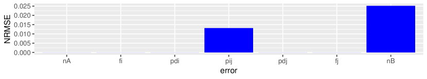
Figure 4: Error rates of the case solved with all parameters relaxed.

We first run the solving of this pairing problem with all the relaxation parameters relaxed: $\nu^{A}=\allowbreak\phi^{A}=\allowbreak\delta^{A}=\allowbreak\gamma=\allowbreak\delta^{B}=\allowbreak\phi^{B}=\allowbreak\nu^{B}=1$. The solver explores all the possible 128 combinations of hypothesis. 8 valid solutions are found, with the one minimizing the weighted error being based on hypothesis: $\hat{n}_{A}=n_{A},\allowbreak\hat{f}_{i}=f_{i},\allowbreak\hat{pd}_{i}=pd_{i},\allowbreak\hat{pd}_{j}=pd_{j}$ and $\hat{f}_{j}=f_{j}$. This solution accepts the required count of dwellings $\hat{n}_{A}=n_{A}$, preserves the frequencies for dwellings and households $f_{i}$ and $f_{j}$, the distribution of degrees $pd_{i}$ and $pd_{j}$, but does not preserve the pairing probabilities $p_{i,j}$ nor the count of households $\hat{n}_{B}$. The algorithm generates a population of exactly $\hat{n}_{A}=130000$ dwellings but $\hat{n}_{B}=123016$ households (slightly more than expected). The repartition of error rates (Fig. 4) shows that the solving process reported biases on pairing probabilities and count of entities $n_{B}$. Tables 21 and 22 in annex, in pages 21 and 22 depict excerpts of the solved probabilistic perspective and the discrete perspective. We depict in table 16 an excerpt of the generated population.

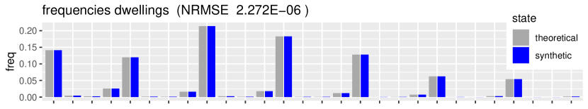
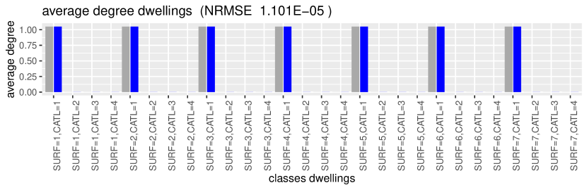
Figure 5: Comparison between expected and solved variables for dwellings in the fully relaxed experiment: (top) frequencies for classes, (bottom) average degrees.

The frequencies and average degrees of dwellings (Fig 5) are preserved with a very high precision. Even the numerous classes of dwellings for which the degree is 0 are represented as expected, demonstrating the capability of the solver based on our theoretical framework to deal with the zero cells. The measured NRMSE($f_{i}$) and NRMSE($d_{i}$) are very low, and correspond to the necessary rounding of probabilities introduced during solving.

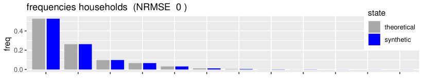
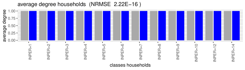
Figure 6: Comparison between expected and solved variables for households in the fully relaxed experiment: (top) frequencies for classes, (bottom) average degrees.

On the side of households depicted in Table 6, the frequencies and average degrees are enforced exactly; here even rounding did not lead to any error, as the probabilities in the distribution of degree were binary (1 or 0) rather than continuous. Note that even the frequencies which were null or nearly null were processed without specific workaround.

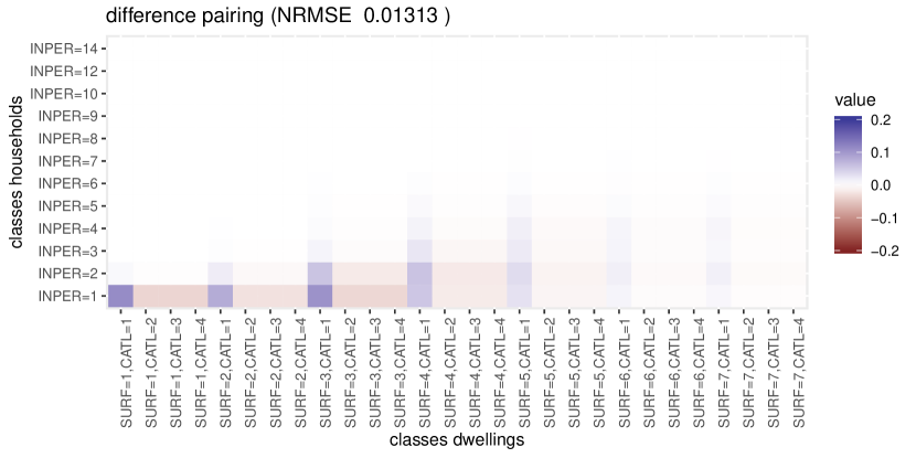
Figure 7: Pairing probabilities: heat-map of the differences (red) for less values than expected, blue for more.

The pairing probabilities (Fig. 7) show where the probabilities were mainly modified: there are slightly more links created between dwellings having CATL=1 (main residences) and small households (INPER=1 or 2). In order to keep the frequencies of households classes similar, this additional proportion of links was balanced during computation by a small diminution of the other links created for each line in order to enforce the marginals (and thus the frequencies for households); those last have no impact, as they only modify the proportions of slots for classes which have degree 0; as empty slots are not visible in the synthetic population, this will be neutral for the model. This correction of these probabilities was done because we provided contradictory information as an input: the expected degrees for dwellings depend on the category CATL which determines whether they are empty or not, but the pairing probabilities we provided only do depend on the surface SURF of the dwelling; we should have provided pairing probabilities with a null probability of a link connecting any dwelling having CATL different from 1. This constitutes an example of a correction of a bias which is desirable, and does not really introduce any bias in the synthetic population.

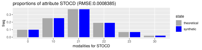
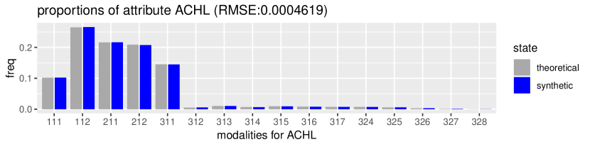
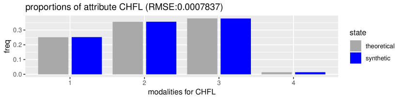
Figure 8: Comparison between the initial and synthetic distributions of free variables for dwellings in the fully relaxed case. From top to bottom: detailed occupancy status (STOCD), date of building construction (ACHL), type of heater (CHFL).

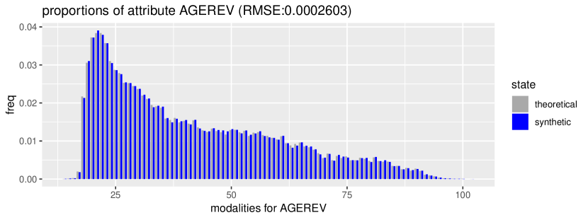
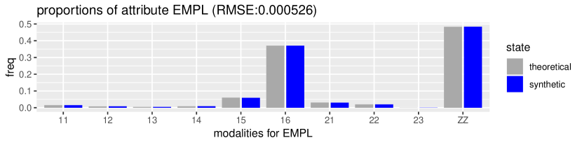
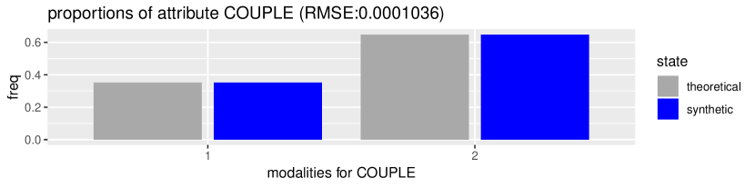
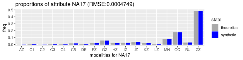
Figure 9: Comparison between the initial and synthetic distributions of free variables for households in the fully relaxed case. From top to bottom: Detailed age of the head of the household (AGEREV), employment status (EMPL), marital status (COUPLE), type of job (NA17)

If the solving process preserves as expected the constrained distributions of classes for the classes controlled during solving, there are other variables for dwellings and households which are not controlled. We depict in Fig. 8 and 9 the difference between initial distributions in the sample and the generated ones for dwellings. The error quantification are low enough for any usage. The absence of difference for the detailed variable AGEREV is of interest, as it has very similar distributions and very good aggregate statistics despite its many classes. The initial distribution of these weights is maintained because the generation phases selects randomly the entities to copy proportionally to their weights, and also because the frequencies of the controlled variables are enforced. If the proportion of empty dwellings was to be modified by the pairing algorithm, this distribution would naturally be biased in the same way according to the statistical dependencies present in the micro sample.

id.A	ACHL	CATL	CHFL	NBPI	SURF
102565	112	1	4	5	5
63140	211	1	1	3	3
84201	112	1	1	3	4
110738	111	1	2	5	5
108720	211	1	1	8	5
10711	212	1	3	1	1
31670	211	1	2	3	2
74560	212	1	2	5	4
58291	325	1	3	1	3
39660	212	4	3	2	2
103030	212	1	2	5	5
78253	212	1	1	3	4
87708	212	1	2	1	4
52353	212	1	1	2	3
64265	211	1	3	1	3
85993	112	1	2	3	4
27427	111	1	3	2	2
88197	211	1	2	4	4
66125	211	1	1	1	3
114772	212	1	1	5	6
89387	212	1	3	3	4
91534	112	1	3	4	4
98405	211	1	1	5	5
79872	211	1	1	3	4
26858	112	1	1	2	2
106756	212	1	1	5	5
33034	111	1	2	2	2
9885	311	1	3	1	1
58510	212	1	3	2	3
9148	311	1	3	1	1
28266	212	1	3	2	2
13022	324	1	3	2	1
3756	311	1	3	1	1
33036	212	1	3	2	2
36126	112	1	3	2	2
128526	111	1	2	6	7
127527	112	1	3	7	7
10483	311	1	3	1	1
56975	211	1	1	2	3
124214	112	1	2	3	7
113171	211	1	2	4	5
1440	315	1	1	1	1
51318	212	1	2	1	3
39821	112	4	2	1	2
56995	211	1	3	2	3
69621	211	4	2	3	3
109885	211	1	1	3	5
103719	112	1	2	5	5
6418	325	1	1	1	1
39588	212	4	1	2	2
…	…	…	…	…	…

id.A	id.B
102565	234203
63140	226070
84201	197463
110738	209788
108720	236952
10711	173346
31670	157397
74560	148814
58291	146090
39660
103030	234345
78253	130227
87708	148775
52353	246276
64265	248992
85993	136302
27427	175290
88197	132970
66125	161881
114772	236386
89387	211231
91534	176206
98405	226251
79872	149952
26858	146315
106756	240091
33034	175591
9885	156578
58510	197153
9148	150927
28266	161260
13022	143012
3756	163184
33036	179380
36126	185435
128526	249872
127527	208320
10483	150333
56975	194862
124214	250556
113171	205322
1440	174686
51318	204638
39821
56995	184359
69621
109885	234174
103719	199647
6418	193356
39588
…	…

id.B	AGEREV	COUPLE	EMPL	INPER	NA17
234203	58	1	16	3	OQ
226070	41	2	16	2	GZ
197463	37	1	12	2	MN
209788	64	1	ZZ	2	ZZ
236952	38	1	16	3	OQ
173346	37	2	ZZ	1	ZZ
157397	41	2	16	1	OQ
148814	50	2	ZZ	1	ZZ
146090	21	2	ZZ	1	ZZ
234345	31	1	15	3	OQ
130227	69	2	ZZ	1	ZZ
148775	29	2	16	1	MN
246276	27	1	ZZ	4	ZZ
248992	33	2	16	5	OQ
136302	54	2	16	1	HZ
175290	20	2	ZZ	1	ZZ
132970	28	2	16	1	GZ
161881	44	2	12	1	MN
236386	32	2	ZZ	3	ZZ
211231	37	1	16	2	C5
176206	58	2	16	1	GZ
226251	64	1	ZZ	2	ZZ
149952	74	2	ZZ	1	ZZ
146315	69	2	ZZ	1	ZZ
240091	54	2	21	4	OQ
175591	55	2	ZZ	1	ZZ
156578	61	1	16	1	KZ
197153	33	1	16	2	MN
150927	65	2	ZZ	1	ZZ
161260	23	2	16	1	JZ
143012	20	2	ZZ	1	ZZ
163184	33	1	16	1	JZ
179380	21	2	ZZ	1	ZZ
185435	39	2	ZZ	1	ZZ
249872	34	1	ZZ	5	ZZ
208320	36	2	ZZ	2	ZZ
150333	23	2	ZZ	1	ZZ
194862	38	1	ZZ	2	ZZ
250556	47	1	16	5	OQ
205322	32	2	16	2	LZ
174686	21	2	16	1	GZ
204638	33	2	16	2	C5
184359	61	2	ZZ	1	ZZ
234174	32	1	ZZ	3	ZZ
199647	68	2	ZZ	2	ZZ
193356	70	2	ZZ	1	ZZ
…	…	…	…	…	…

Table 16: Excerpt of the synthetic population generated for Lille. (left) Population A (dwellings). (center) Links between A and B (here: composition links). (right) Population B (households). Empty lines correspond to empty dwellings which have no corresponding household.

We applied this solution at the scale of Lille with only one constraint for summary statistics $f_{i}$ and $f_{j}$ for the entire city, because our initial sample is weighted so to be relevant at the local scale. The same approach might be used on each distinct statistical small area with different values if the initial sample is not statistically representative, as was done in the reweighing solutions 1.3.1.

4.3 Impact of relaxation parameters

We saw the result of resolution with all the relaxation parameters being relaxed, so the solver was free to explore all the possible solutions and retain the one minimizing the weighted error. We now test what happens if we constrain the case on pairing probabilities, so relaxation parameters are $\gamma=0$ and $\nu^{A}=\allowbreak\phi^{A}=\allowbreak\delta^{A}=\allowbreak\phi^{B}=\allowbreak\delta^{B}=\allowbreak\nu^{B}=1$.

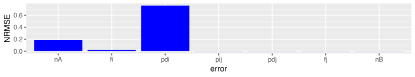
Figure 10: Error rates of the case solved with the constraint $p_{i,j}=\hat{p}_{i,j}$.

This time, after the analysis of 16 valid solutions, the solver ends with a best solution based on hypothesis $\hat{f}_{i}=f_{i}$,$\hat{p}_{i,j}=p_{i,j}$, $\hat{f}_{j}=f_{j}$ and $\hat{n}^{B}=n^{B}$. The synthetic population contains $\hat{n}_{A}=153850$ (more than expected) and $\hat{n}_{B}=120000$. We depict in figure 10 the errors obtained at the end of the process. The constraint on the pairing probabilities is enforced, with only a very low error rate due to rounding. But the errors obtained this time are high where the relaxation parameters allowed it. We plot in figure LABEL:fig_lille_pairing_degree_dwelling the detail of the average degree and distribution of degrees. The frequencies of classes were modified a lot: all the classes leading to degree 0 (those with CATL!=1) are slightly over represented in relative frequencies, and their theoretical degree was shifted from 0 to 2. In other terms, because the pairing probabilities were requiring proportions of links even when no or few entities and slots were supposed to be created for them, the algorithm distorted these probabilities in order to create the necessary slots and links. This huge distortion of the input parameters is probably not desirable in practice, as we try to enforce the pairing probabilities which are not consistent for some classes. In order to use a population, we would fix the pairing probabilities. In the scope of this paper however, this experiment demonstrated how the solver and theoretical frameworks provide the user with the freedom do define where to introduce biases, and enables to quantify the quality of the result.

$n^{A}$	$n^{B}$	$\nu^{A}$	$\phi^{A}$	$\delta^{A}$	$\gamma$	$\delta^{B}$	$\phi^{B}$	$\nu^{B}$	$\hat{n}_{A}$	$\hat{n}_{B}$	nrmse.nA	nrmse.fi	nrmse.pdi	nrmse.pij	nrmse.pdj	nrmse.fj	nrmse.nB	solving time	generation time
130000	120000	1	1	1	1	1	1	1	130000	123016	0.00	0.00	0.00	0.01	0.00	0.00	0.03	4.14	14
130000	120000	1	1	1	1	1	1	0	114286	120000	0.12	0.00	0.00	0.01	0.00	0.00	0.00	4.17	10
130000	120000	1	1	1	1	1	0	1	130000	123016	0.00	0.00	0.00	0.01	0.00	0.00	0.03	3.19	14
130000	120000	1	1	1	1	0	1	1	130000	123016	0.00	0.00	0.00	0.01	0.00	0.00	0.03	3.47	14
130000	120000	1	1	1	0	1	1	1	153841	120000	0.18	0.02	0.76	0.00	0.00	0.00	0.00	4.97	39
130000	120000	1	1	0	1	1	1	1	130000	123016	0.00	0.00	0.00	0.01	0.00	0.00	0.03	2.21	14
130000	120000	1	0	1	1	1	1	1	130000	123016	0.00	0.00	0.00	0.01	0.00	0.00	0.03	3.33	15
130000	120000	0	1	1	1	1	1	1	130000	123016	0.00	0.00	0.00	0.01	0.00	0.00	0.03	4.20	15
130000	120000	0	1	0	1	1	1	1	130000	123016	0.00	0.00	0.00	0.01	0.00	0.00	0.03	2.63	15
130000	120000	1	1	0	1	1	1	0	114286	120000	0.12	0.00	0.00	0.01	0.00	0.00	0.00	2.44	11
130000	120000	0	0	1	1	1	1	1	130000	123016	0.00	0.00	0.00	0.01	0.00	0.00	0.03	3.86	15
130000	120000	0	0	1	1	1	1	1	130000	123016	0.00	0.00	0.00	0.01	0.00	0.00	0.03	3.85	14
130000	120000	1	0	0	1	1	1	1	130000	123016	0.00	0.00	0.00	0.01	0.00	0.00	0.03	2.92	15
130000	120000	1	1	0	0	1	1	1	130000	123016	0.00	0.00	0.00	0.01	0.00	0.00	0.03	2.86	16
130000	120000	1	1	1	0	0	1	1	153865	120000	0.18	0.02	0.76	0.00	0.00	0.00	0.00	4.53	42
130000	120000	1	1	1	1	0	0	1	130000	123016	0.00	0.00	0.00	0.01	0.00	0.00	0.03	4.69	15
130000	120000	0	0	0	1	1	1	1	130000	123016	0.00	0.00	0.00	0.01	0.00	0.00	0.03	2.67	16
130000	120000	1	0	0	0	1	1	1	130000	123016	0.00	0.00	0.00	0.01	0.00	0.00	0.03	3.50	16
130000	120000	1	1	0	0	0	1	1	130000	123016	0.00	0.00	0.00	0.01	0.00	0.00	0.03	2.22	15
130000	120000	1	1	0	0	0	1	1	130000	123016	0.00	0.00	0.00	0.01	0.00	0.00	0.03	2.25	15
130000	120000	1	1	1	0	0	0	1	153865	120000	0.18	0.02	0.76	0.00	0.00	0.00	0.00	5.96	40
130000	120000	1	1	1	1	0	0	0	114286	120000	0.12	0.00	0.00	0.01	0.00	0.00	0.00	4.92	12
130000	120000	1	0	1	0	0	0	0	-	-	-	-	-	-	-	-	-	0.03	-
130000	120000	1	0	0	0	0	0	0	-	-	-	-	-	-	-	-	-	0.04	-
130000	120000	1	1	1	0	0	0	0	153865	120000	0.18	0.02	0.76	0.00	0.00	0.00	0.00	4.15	41
130000	120000	0	1	1	0	0	1	1	130000	56633	0.00	0.02	0.76	0.01	0.00	0.00	0.53	5.32	25
130000	120000	0	1	1	1	1	1	1	130000	123016	0.00	0.00	0.00	0.01	0.00	0.00	0.03	4.32	16
130000	120000	0	0	1	1	1	1	1	130000	123016	0.00	0.00	0.00	0.01	0.00	0.00	0.03	3.97	16
130000	120000	0	0	0	1	1	1	1	130000	123016	0.00	0.00	0.00	0.01	0.00	0.00	0.03	2.76	15
130000	120000	1	0	0	1	0	0	1	130000	123016	0.00	0.00	0.00	0.01	0.00	0.00	0.03	4.29	16
130000	120000	1	1	1	0	1	1	1	153841	120000	0.18	0.02	0.76	0.00	0.00	0.00	0.00	5.18	40

Table 17: Exploration of the space of solvers’ parameters applied on the Lille case: target population sizes $n_{A}$ and $n_{B}$, relaxation parameters, resulting synthetic population sizes $\hat{n}_{A}$ and $\hat{n}_{B}$, Normalized Rooted Mean Squarred Errors, solving and generation time in seconds.

We test other combinations of relaxation parameters to illustrate the potential results and demonstrate the capability of our method to assign the biases in different places of the problem, thus enabling a user to enforce at least part of his constraints. The results are depicted in table 17. When a relaxation parameter set to 0 is leading to fail, then all the combinations involving the same parameter also fails. Note that the computation is sometimes not possible because the case if considered over-constrained, and is then refused. Note the generation time is also depicted in this table, and remains below one minute.

5 Discussion

5.1 Summary

We tackle the problem of generating a synthetic population made of entities of type A and B in which entities A and B can be connected together with 0, 1 or more links according to their characteristics, and A and B enforce given distributions of frequencies.

We proposed the semantics and formats for the input data (2) made of weighted samples of A and B, definition of classes $i$ and $j$ made of combinations of modalities of variables for A and B, expected frequencies for these classes $f_{i}$ and $f_{j}$, distribution of degrees encoded as conditional probabilities for an entity A or B to have degree $n$ given it belongs to class $i$ or $j$, and pairing constraints in the form of a joint probability table between classes $i$ and $j$. We proposed a theoretical framework (3) to analyze and solve the pairing problem, which is made of variables describing the probabilistic perspective of the pairing problem and the variables describing the discrete counterpart required for generation. We defined how each variable is produced from input data and/or its relationship with other variables in the form of 24 equations. Our approach is based on the principle that the pairing problem is an over-constrained problem which requires an approximate solution relaxed according to relaxation parameters, which can be found by an analytic process. We proposed an example of a solver which was demonstrated able to solve the toy and real-size pairing problems. We illustrated how this solver proposes solutions enforcing various combinations of relaxation parameters on the same user data. We explained and demonstrated (4) how the generation of a synthetic population based on this theoretical framework becomes a direct process, mainly because our approach involves the removal of any inconsistency between data in the probabilistic and discrete perspectives at the solving stage.

We illustrated this approach with two examples. A toy example of dwellings used for the illustration of the pairing problems, in which the initial samples were actually generated randomly. We then applied our methodology to a real-size case for the reconstruction of dwellings and households in the city of Lille in France. We demonstrated that the controlled variables are enforced when the relaxation parameters require and, and that the variables not controlled by the algorithm are also enforced accordingly.

In order to facilitate replication and reusal of this method, we publish along this paper the open-source, documented R package which was used for the experiments. Instead of some past methods which delivered hard-coded software [19, 21] or none, we propose it as a fully generic software. It is shared in https://github.com/samthiriot/gosp.dpp.

We denoted this method Direct Probabilistic Pairing. ”Pairing” stands as the focus of the algorithm, which is not to be based or not on samples, but focuses on the creation of links between entities. ”Direct” refers to the direct generation of the population after solving, which avoid the iterative linking solutions proposed in past sample-free methods. ”Probabilistic” stands because it accepts several inputs formulated as probabilities and analyses the pairing problem in a probabilistic framework.

5.2 Position in the state of the art

Positioning our proposal in the state of the art in the generation of synthetic populations stands as an open discussion, as we do not tackle the very same problem as these studies. Our proposal notably differs in its goal, input data, the method, and application scope.

Regarding the goal, we focus on the creation of any population made of entities A and B linked together with $n:n$ relationships (that is, each a and b can have 0 to n links with the other type). The SR methods so far focus on the only generation of $1:n$ links with $n>0$ (such as between households and persons). The notable exception is the method from Thiriot et al. [40] which generates $n:n$ links. Note that our method enables the creation of no link for some classes whilst preserving the initial distribution of entities.

About the input data, sample-based SR methods do require micro samples of A and B which should share a common identifier; we underlined (1.3.3) how this constraints is likely to be satisfied in very specific datasets only. Sample-free methods require as inputs summary data for A and B and joint probabilities for pairing. We here ask for a mix between both, as we do require weighted micro samples for A and B, and summary data for pairing probabilities and distributions of degrees. Note that the micro samples we require, as they do not have a strong constraint of link between them, might be generated from summary data (as was done for our initial example of dwellings and households used as illustration in 3), thus also making in practice DPP being another sample-free method.

Regarding the method, the sample-based methods rely on a fit-and-generate scheme to reweight micro samples of dwellings composing households. Sample-free methods generate A and B, then iteratively create links between A and B. Our method also relies on a solve-and-generate scheme, where solving analytically the entire system (including the discrete version) makes the generation step direct. Different methods lead to different allocations of errors: sample-based methods introduce errors in the weights of persons (when they control household), household (when they control person) or split the errors when they control both levels at a time (1.3.1). Sample-free methods introduce errors depending on their algorithm (1.3.4). DPP introduces biases in different locations according to relaxation parameters defined by the user. We claim this originality is a benefit of our method, because it enables the usage of the same framework and algorithm in different scenarios were preserving the sizes and/or frequencies and/or degrees and/or pairing are of importance or not.

Concerning the application scope, our method can be applied to any type of entities A and B to be connected together. We illustrated here the application on dwellings and households, which was not tackled yet in the literature. The sample-based methods are limited to the cases where the composition relationship is already known (in practice, households and persons collected during the census - see 1.3.3). The sample-free methods were designed for the specific case of households and persons, but can likely be easily extended to any other kind of $0:n$ relationships with minor changes in the methodology. While we claim the genericity of our approach, it also might make this approach less relevant for specific cases. The existing sample-free methods developed for the creation of households made of persons (1.3.4) do not only create households-person links, but also create consistent households made of persons having socio coherent demographic characteristics (such as for spouses ages, etc.). Our method focus on the sole consistency between the sources’ and targets’ characteristics of each link (dyadic approach in social network analysis), but does not constraints anything about the other dependencies. As a consequence, our solution is generic, but is not suitable for the specific case of creating coherent groups of entities composed inside another entity.

Provided these many facets and differences, it is difficult to assign DPP to the current categories of ”sample-based” and ”sample-free” synthetic reconstruction methods. Like sample-free methods, we explicitly create links between two types of entities and accept the related input parameters. Like sample-based methods, we use a solve-and-generate pattern in order to fix inconsistencies prior to generation. A way to see the DPP method is to see it as an extension of the fitting approach used so far on sample-based SR methods (with the frequencies $f_{i}$ and $f_{j}$ being the two multi-way tables fit in these methods) which manages pairing like in the sample-free SR methods but with an analytical rather than algorithmic solving.

5.3 Solver

We see the core of our proposal as the theoretical framework we highlighted. In the same way Beckman only introduced IPF as one tool to solve the reweighing problem he had identified [15], we only consider the solver we introduced as a tool necessary for dealing with the problem which might be replaced if a better tool is found. This first version suffers many limitations. This solver is not able to explore trade-offs; for instance the generated population will contain the exact count of agents $\hat{n}_{A}=n_{A}$, or of $\hat{n}_{B}=n_{B}$, or both, but will not propose an intermediate solution with the error being split between $\hat{n}_{A}$ and $\hat{n}_{B}$. Additional research should explore how to enhance this process, either by the analytic solving of the problem understood as the minimization of the aggregate summed error, using an iterative solving of this problem, or (inspired by combinatorial optimization methods) using any state-of-the-art optimization method like genetic algorithms to solve the various variables.

5.4 Research directions

A main originality of our proposal is to fit the entire system of frequencies, degrees and links all together, prior to generation. Another innovation is to formulate the integer version of the fitted problem and also solve it immediately in a consistent way. As a consequence, the generation stage is free of errors. We claim this enables to master errors and keep free of allocating them where preferred, instead of discovering the errors after generation.

Our initial framing of the pairing problem and our theoretical formulation induce limits which we intend to question in future research. We only considered the creation of populations made of two types of entities after reweighing of micro samples. Can we link entities of one type only, for instance to create social links between entities? Can we chain several generations with DPP in order to create multi-level synthetic populations like dwellings linked with appliances, dwellings with households, households made of persons?

We consider the Generation of Synthetic Populations as a set of methods and tools which tackle different problems depending to the initial data available, the expectations of the model and simulation experiment, and the constraints the user wishes to enforce. This DPP proposal stands a solution complementary of the state of the art, and not in complete opposition with past methods.

We designed this method so it is generic. In order to challenge and demonstrate this genericity, this algorithm should be applied to different variations of the pairing problem such as the creation of horizontal links (such as social structure) instead of compositions ones, and to different applications including other types of entities. The extrapolation of this theoretical framework to the creation of groups instead of pairs is feasible but would require further investigation.

6 Annex

	ACHL	CATL	CHFL	HLML	IPONDL	NBPI	SURF
1	211	1	3	2	3.71	5	5
2	211	1	3	2	3.71	5	5
3	211	1	3	2	3.71	3	5
4	211	1	3	2	3.71	3	5
5	314	1	2	2	0.98	4	6
6	311	1	3	2	0.98	2	2
7	212	1	3	2	3.23	1	2
8	311	1	3	2	3.23	2	3
9	112	1	2	2	3.32	2	2
10	311	1	3	2	3.16	3	4
11	211	1	3	2	3.23	1	1
12	212	1	2	2	3.41	2	1
13	112	1	1	2	3.23	2	3
14	212	1	3	2	0.98	3	3
15	312	1	3	2	3.16	3	4
16	211	1	1	2	3.32	6	7
17	112	1	2	1	3.23	3	6
18	212	1	3	2	3.23	2	2
19	311	1	3	2	0.98	2	3

Table 18: Excerpt of the sample of dwellings provided by INSEE. The sample contains variables ACHL (year of achievement), CATL (occupancy status), CHFL (type of heater), HLML (social housing), NBPI (count of rooms) and SURF (surface). The column IPONDL contains the weights of the sample.

	AGEREV	AGEREVQ	COUPLE	EMPL	INPER	NA17	IPONDI
1	48	45	1	16	2	OQ	3.46
2	53	50	2	ZZ	1	ZZ	3.59
3	18	15	2	ZZ	1	ZZ	1.03
4	28	25	2	16	2	GZ	3.86
5	32	30	1	16	2	JZ	3.42
6	21	20	2	ZZ	1	ZZ	1.03
7	48	45	2	16	1	JZ	1.09
8	21	20	2	ZZ	3	ZZ	1.03
9	18	15	2	ZZ	1	ZZ	0.99
10	18	15	2	ZZ	1	ZZ	0.85
11	79	75	1	ZZ	2	ZZ	3.81
12	39	35	2	16	1	OQ	3.83
13	19	15	2	ZZ	1	ZZ	3.39
14	18	15	2	15	1	MN	1.03
15	24	20	1	16	3	HZ	3.51
16	63	60	1	ZZ	2	ZZ	1.09
17	38	35	1	ZZ	2	ZZ	3.38
18	75	75	2	ZZ	1	ZZ	1.19
19	92	90	1	ZZ	2	ZZ	3.61

Table 19: Excerpt of the sample of households provided by INSEE. AGEREV encodes the detailed age, AGEREVQ the age encoded in a quinquenal way, COUPLE the marital status, EMPL the employment status, INPER the count of persons in the household, NA17 (economical activity). IPONDI encodes the weight.

$\text{Cla}_{i}^{A}$ SURF=1,CATL=1 SURF=1,CATL=2 SURF=1,CATL=3 SURF=1,CATL=4 SURF=2,CATL=1 SURF=2,CATL=2 SURF=2,CATL=3 SURF=2,CATL=4 SURF=3,CATL=1 … $f_{i}$ 0.1412 0.004396 0.002261 0.02554 0.1196 0.001501 0.001104 0.01605 0.2136 … 1 $\tilde{d}_{i}$ 1.05 6.661E-16 6.661E-16 6.661E-16 1.05 6.661E-16 6.661E-16 6.661E-16 1.05 … $p_{i}$ 0.03916 0.03916 0.03916 0.03916 0.03319 0.03319 0.03319 0.03319 0.05926 … 1 $\text{Cla}_{j}^{B}$ $f_{j}$ $\tilde{d}_{j}$ $p_{j}$ $j/i$ 1 2 3 4 5 6 7 8 9 … INPER=1 0.5263 1 0.5263 1 0.03699 0.03699 0.03699 0.03699 0.02637 0.02637 0.02637 0.02637 0.03511 … INPER=2 0.2624 1 0.2624 2 0.001958 0.001958 0.001958 0.001958 0.005774 0.005774 0.005774 0.005774 0.01861 … INPER=3 0.09772 1 0.09773 3 0.0001402 0.0001402 0.0001402 0.0001402 0.0007214 0.0007214 0.0007214 0.0007214 0.00337 … INPER=4 0.0662 1 0.0662 4 4.969E-05 4.969E-05 4.969E-05 4.969E-05 0.0002275 0.0002275 0.0002275 0.0002275 0.00138 … INPER=5 0.03061 1 0.03059 5 2.429E-05 2.429E-05 2.429E-05 2.429E-05 5.813E-05 5.813E-05 5.813E-05 5.813E-05 0.0005401 … INPER=6 0.01119 1 0.0112 6 5.651E-17 5.651E-17 5.651E-17 5.651E-17 3.1E-05 3.1E-05 3.1E-05 3.1E-05 0.0001903 … INPER=7 0.003476 1 0.003476 7 5.651E-17 5.651E-17 5.651E-17 5.651E-17 4.8E-06 4.8E-06 4.8E-06 4.8E-06 2.873E-05 … INPER=8 0.001292 1 0.001291 8 5.651E-17 5.651E-17 5.651E-17 5.651E-17 2.427E-06 2.427E-06 2.427E-06 2.427E-06 1.698E-05 … INPER=9 0.0005671 1 0.0005671 9 5.651E-17 5.651E-17 5.651E-17 5.651E-17 5.651E-17 5.651E-17 5.651E-17 5.651E-17 6.599E-06 … INPER=10 0.0001078 1 0.0001078 10 5.651E-17 5.651E-17 5.651E-17 5.651E-17 5.651E-17 5.651E-17 5.651E-17 5.651E-17 5.651E-17 … INPER=12 6.155E-05 1 6.154E-05 11 5.651E-17 5.651E-17 5.651E-17 5.651E-17 5.651E-17 5.651E-17 5.651E-17 5.651E-17 5.651E-17 … INPER=14 3.104E-05 1 3.104E-05 12 5.651E-17 5.651E-17 5.651E-17 5.651E-17 5.651E-17 5.651E-17 5.651E-17 5.651E-17 5.651E-17 … 1 1 1

Table 20: Probabilistic view of the pairing problem of dwellings and households in Lille before resolution. These values reflect initial user parameters and are not consistent.

$\text{Cla}_{i}^{A}$ SURF=1,CATL=1 SURF=1,CATL=2 SURF=1,CATL=3 SURF=1,CATL=4 SURF=2,CATL=1 SURF=2,CATL=2 SURF=2,CATL=3 SURF=2,CATL=4 SURF=3,CATL=1 … $\hat{f_{i}}$ 0.1412 0.004392 0.002262 0.02555 0.1196 0.0015 0.001108 0.01605 0.2136 … 1 $\hat{\tilde{d}}_{i}$ 1.05 0 0 0 1.05 0 0 0 1.05 … $\hat{p}_{i}$ 0.1566 0 0 0 0.1327 0 0 0 0.237 … 1 $\text{Cla}_{j}^{B}$ $\hat{f}_{j}$ $\hat{\tilde{d}}_{j}$ $\hat{p}_{j}$ $j/i$ 1 2 3 4 5 6 7 8 9 … INPER=1 0.5263 1 0.5263 1 0.1479 0 0 0 0.1055 0 0 0 0.1404 … INPER=2 0.2624 1 0.2624 2 0.007836 0 0 0 0.0231 0 0 0 0.07445 … INPER=3 0.09772 1 0.09772 3 0.0005609 0 0 0 0.002886 0 0 0 0.01348 … INPER=4 0.0662 1 0.06619 4 0.0001951 0 0 0 0.0009105 0 0 0 0.00552 … INPER=5 0.03061 1 0.03061 5 9.755E-05 0 0 0 0.0002357 0 0 0 0.002162 … INPER=6 0.01119 1 0.01119 6 0 0 0 0 0.0001219 0 0 0 0.0007641 … INPER=7 0.003476 1 0.003479 7 0 0 0 0 1.626E-05 0 0 0 0.0001138 … INPER=8 0.001292 1 0.001293 8 0 0 0 0 8.129E-06 0 0 0 6.503E-05 … INPER=9 0.0005671 1 0.0005609 9 0 0 0 0 0 0 0 0 2.439E-05 … INPER=10 0.0001078 1 0.0001057 10 0 0 0 0 0 0 0 0 0 … INPER=12 6.155E-05 1 6.503E-05 11 0 0 0 0 0 0 0 0 0 … INPER=14 3.104E-05 1 3.252E-05 12 0 0 0 0 0 0 0 0 0 … 1 1 1

Table 21: Probabilistic view of the solved pairing problem with population sizes $n^{A}=130000$ and $n^{B}=120000$. Relaxation parameters are $\nu^{A}=\allowbreak\phi^{A}=\allowbreak\delta^{A}=\allowbreak\gamma=\allowbreak\delta^{B}=\allowbreak\phi^{B}=\allowbreak\nu^{B}=1$. The population generated sizes $\hat{n}^{A}=130000$ and $\hat{n}^{B}=123016$.

$\text{Cla}_{i}^{A}$ SURF=1,CATL=1 SURF=1,CATL=2 SURF=1,CATL=3 SURF=1,CATL=4 SURF=2,CATL=1 SURF=2,CATL=2 SURF=2,CATL=3 SURF=2,CATL=4 SURF=3,CATL=1 … $\hat{c_{i}}$ 18351 571 294 3321 15552 195 144 2087 27769 … 130000 $\hat{\tilde{d}}_{i}$ 1.05 0 0 0 1.05 0 0 0 1.05 … $\hat{n}_{i}$ 19269 0 0 0 16330 0 0 0 29157 … 123016 $\text{Cla}_{j}^{B}$ $\hat{c}_{j}$ $\hat{\tilde{d}}_{j}$ $\hat{n}_{j}$ $j/i$ 1 2 3 4 5 6 7 8 9 … INPER=1 64744 1 64744 1 18200 0 0 0 12974 0 0 0 17276 … INPER=2 32284 1 32284 2 964 0 0 0 2842 0 0 0 9159 … INPER=3 12021 1 12021 3 69 0 0 0 355 0 0 0 1658 … INPER=4 8143 1 8143 4 24 0 0 0 112 0 0 0 679 … INPER=5 3766 1 3766 5 12 0 0 0 29 0 0 0 266 … INPER=6 1377 1 1377 6 0 0 0 0 15 0 0 0 94 … INPER=7 428 1 428 7 0 0 0 0 2 0 0 0 14 … INPER=8 159 1 159 8 0 0 0 0 1 0 0 0 8 … INPER=9 69 1 69 9 0 0 0 0 0 0 0 0 3 … INPER=10 13 1 13 10 0 0 0 0 0 0 0 0 0 … INPER=12 8 1 8 11 0 0 0 0 0 0 0 0 0 … INPER=14 4 1 4 12 0 0 0 0 0 0 0 0 0 … 123016 123016 123016

Table 22: Discrete view of the solved pairing problem with population sizes $n^{A}=130000$ and $n^{B}=120000$. Relaxation parameters are $\nu^{A}=\allowbreak\phi^{A}=\allowbreak\delta^{A}=\allowbreak\gamma=\allowbreak\delta^{B}=\allowbreak\phi^{B}=\allowbreak\nu^{B}=1$. The population generated sizes $\hat{n}^{A}=130000$ and $\hat{n}^{B}=123016$.

6.1 Source and preparation of micro samples

Micro samples for dwellings and households come from the 2014 census information provided by the French national institute for statistics named INSEE. The datasets are freely available on their website. We loaded them from CSV format into R [48] using the sqldf package [51] which enables the selection of the records of interest to our case.

The sample for population A is the weighted sample of dwellings. We download from the INSEE website the public dataset named ”logements” (dwellings) [52].of zone B (north of France) We retain only the elements relevant to our case: we keep elements of the city of Lille (variable ’COMMUNE’ equal to 59350); we exclude the dwellings classified as being specific (CATL different of 2 and 4). The resulting dataset contains 51480 entities. We present in table 18 a few lines of this sample.

The sample for population B is a weighted sample of households [53]. We download from the INSEE website the data sets named ”logements” of zone B. We retain only the elements relevant to the area of the city of Lille (variable ’CANTVILLE’ = 5997). The original dataset is structured with several lines per representative household sharing the same household identifier. We focus on the only lines representing the head of household, that is records having ‘LPRM‘=1. The resulting dataset contains 46138 entities.

References

-
[1]
G. H. Orcutt, A New
Type of Socio-Economic System, The Review of Economics and Statistics
39 (2) (1957) 116.
doi:10.2307/1928528.
URL http://www.jstor.org/stable/1928528?origin=crossref - [2] J. Merz, Microsimulation - A survey of principles, developments and applications, International Journal of Forecasting 7 (1) (1991) 77–104. doi:10.1016/0169-2070(91)90035-T.
- [3] E. Baroni, M. Richiardi, Orcutt’s Vision, 50 years on, Tech. rep., LABORatorio R. Revelli, Centre for Employment Studies (2007).
-
[4]
R. Lovelace, M. Dumont,
Spatial
microsimulation with R., CRC Press, 2016.
URL https://spatial-microsim-book.robinlovelace.net/ - [5] A. J. Heppenstall, A. T. Crooks, L. M. See, M. Batty, Agent-based models of geographical systems, Springer Science & Business Media, 2011.
- [6] N. Gilbert, K. Troitzsch, Simulation for the Social Scientists, Open University Press., 1999.
- [7] D. Phan, F. Amblard, Agent-based Modelling, The Bardwell Press, Oxford, 2007.
- [8] A. Smajgl, O. Barreteau, Empirical Agent-Based Modelling - Challenges and Solutions, Springer-Verlag New York, 2014.
- [9] P. Waddell, UrbanSim - Modeling urban development for land use, transportation, and environmental planning, Journal of the American Planning Association 68 (August) (2002) 297–314. doi:10.1080/01944360208976274.
- [10] M. Balmer, K. Axhausen, K. Nagel, Agent-based demand-modeling framework for large-scale microsimulations, Transport. Res. Rec. J. Transpo (2006) 125–134.
- [11] P. Salvini, E. Miller, ILUTE: an operational prototype of a comprehensive microsimulation model of urban systems, Networks Spatial Econ. 5 (2) (2005) 217—-234.
- [12] E. Amouroux, T. Huraux, F. Sempé, N. Sabouret, Y. Haradji, SMACH: Agent-Based Simulation Investigation on Human Activities and Household Electrical Consumption, Communications in Computer and Information Science 449 (October). doi:10.1007/978-3-662-44440-5.
- [13] S. Thiriot, Z. Lewkovicz, P. Caillou, J.-D. Kant, Referral hiring and labor markets: a computational study, in: Emergent Results of Artificial Economics, Springer, 2011, pp. 15–25.
-
[14]
M. Batty,
Planning
support systems: progress, predictions, and speculations on the shape of
things to come, Tech. rep., University College London – Centre for
Advanced Spatial Analysis (2007).
arXiv:0706.0024,
doi:10.1103/PhysRevE.78.016110.
URL http://www.springerlink.com/index/j3863x4mm7gu8645.pdf - [15] R. J. Beckman, K. A. Baggerly, M. D. McKay, Creating synthetic baseline populations, Transportation Research Part A: Policy and Practice 30 (6) (1996) 415–429.
- [16] K. Müller, K. W. Axhausen, Hierarchical IPF: Generating a synthetic population for Switzerland, Eidgenössische Technische Hochschule Zürich, IVT, 2011.
- [17] W. E. Deming, F. F. Stephan, On a least squares adjustment of a sampled frequency table when the expected marginal totals are known, The Annals of Mathematical Statistics 11 (4) (1940) 427–444.
-
[18]
J. L. Bowman,
A
comparison of population synthesizers used in microsimulation models of
activity and travel demand, Tech. rep. (2004).
URL http://www.jbowman.net/papers/2004.Bowman.Comparison{_}of{_}PopSyns.pdf -
[19]
J. Guo, C. Bhat,
Population
Synthesis for Microsimulating Travel Behavior, Transportation Research
Record: Journal of the Transportation Research Board 2014 (2007) 92–101.
doi:10.3141/2014-12.
URL http://trrjournalonline.trb.org/doi/10.3141/2014-12 - [20] X. Ye, K. Konduri, R. M. Pendyala, B. Sana, P. Waddell, A methodology to match distributions of both household and person attributes in the generation of synthetic populations, in: 88th Annual Meeting of the Transportation Research Board, Washington, DC., 2009.
- [21] K. Müller, K. W. Axhausen, Population synthesis for microsimulation: State of the art, in: 90th Annual Meeting of the Transportation Research Board, ETH Zürich, Institut für Verkehrsplanung, Transporttechnik, Strassen-und Eisenbahnbau (IVT), 2010.
-
[22]
R. Lovelace, M. Birkin, D. Ballas, E. van Leeuwen,
Evaluating the performance
of Iterative Proportional Fitting for spatial microsimulation: new tests for
an established technique, Journal of Artificial Societies and Social
Simulation 18 (2) (2015) 21.
doi:10.18564/jasss.2768.
URL http://jasss.soc.surrey.ac.uk/18/2/21.html - [23] L. Ma, S. Srinivasan, Synthetic population generation with multilevel controls: A fitness-based synthesis approach and validations, Computer-Aided Civil and Infrastructure Engineering 30 (2) (2015) 135–150. doi:10.1111/mice.12085.
- [24] D. R. Pritchard, E. J. Miller, Advances in population synthesis: Fitting many attributes per agent and fitting to household and person margins simultaneously, Transportation 39 (3) (2012) 685–704. doi:10.1007/s11116-011-9367-4.
-
[25]
T. Arentze, H. Timmermans, F. Hofman,
Creating
Synthetic Household Populations: Problems and Approach, Transportation
Research Record: Journal of the Transportation Research Board 2014 (2007)
85–91.
doi:10.3141/2014-11.
URL http://trrjournalonline.trb.org/doi/10.3141/2014-11 - [26] H. Bar-Gera, K. C. Konduri, B. Sana, X. Ye, R. M. Pendyala, Estimating survey weights with multiple constraints using entropy optimization methods, in: Transportation Research Board 88th Annual Meeting, no. 09-1354, 2009.
- [27] J. A. Auld, A. Mohammadian, Efficient methodology for generating synthetic populations with multiple control levels, Transportation Research Record: Journal of the Transportation Research Board 2175 (1) (2010) 138–147.
- [28] R. Lovelace, D. Ballas, ‘Truncate, replicate, sample’: A method for creating integer weights for spatial microsimulation, Computers, Environment and Urban Systems 41 (2013) 1–11. doi:10.1016/j.compenvurbsys.2013.03.004.White.
- [29] A. P. Smith, R. Lovelace, M. Birkin, Population synthesis with quasirandom integer sampling, Jasss 20 (4). doi:10.18564/jasss.3550.
- [30] P. Williamson, M. Birkin, P. H. Rees, Others, The estimation of population microdata by using data from small area statistics and samples of anonymised records, Environment and Planning A 30 (1998) 785–816.
- [31] M. Birkin, A. Turner, B. Wu, A synthetic demographic model of the UK population: Methods, progress and problems, in: Regional Science Association International British and Irish Section, 36th Annual Conference, Citeseer, 2006.
- [32] D. Voas, P. Williamson, An evaluation of the combinatorial optimisation approach to the creation of synthetic microdata, International Journal of Population Geography 6 (5) (2000) 349–366.
- [33] Z. Huang, P. Williamson, A comparison of synthetic reconstruction and combinatorial optimisation approaches to the creation of small-area microdata, Tech. rep. (2001).
- [34] J. Ryan, H. Maoh, P. Kanaroglou, Population synthesis: Comparing the major techniques using a small, complete population of firms, Geographical Analysis 41 (2) (2009) 181–203.
- [35] D. M. Smith, G. P. Clarke, K. Harland, Improving the synthetic data generation process in spatial microsimulation models, Environment and planning. A 41 (5) (2009) 1251.
- [36] F. Gargiulo, S. Ternes, S. Huet, G. Deffuant, An iterative approach for generating statistically realistic populations of households, PLoS One 5 (1) (2010) e8828.
- [37] J. Barthelemy, P. L. Toint, Synthetic population generation without a sample, Transportation Science 47 (2) (2013) 266–279.
- [38] M. Birkin, M. Clarke, SYNTHESIS–a synthetic spatial information system for urban and regional analysis: methods and examples, Environment and planning A 20 (12) (1988) 1645–1671.
- [39] N. Huynh, J. Barthélemy, P. Perez, A heuristic combinatorial optimisation approach to synthesising a population for agent-based modelling purposes, Journal of Artificial Societies and Social Simulation 19 (4). doi:10.18564/jasss.3198.
- [40] S. Thiriot, J.-D. Kant, Generate country-scale networks of interaction from scattered statistics, in: The Fifth Conference of the European Social Simulation Association, Brescia, Italy, 2008.
-
[41]
Z. Lewkovicz, S. Thiriot, P. Caillou,
How detailed should
social networks be for labor market’s models?, in: SNAMAS@AISB 2011, 2011.
URL https://hal.inria.fr/inria-00579620/document - [42] S. Wasserman, K. Faust, Social network analysis, methods and applications, Cambridge: Cambridge University Press, 1994, Ch. Social Net, pp. 3–25.
- [43] D. Voas, P. Williamson, Evaluating goodness-of-fit measures for synthetic microdata, Geographical and Environmental Modelling 5 (2) (2001) 177–200. doi:10.1080/13615930120086078.
- [44] C. B. Read, Freeman—Tukey chi-squared goodness-of-fit statistics, Statistics & probability letters 18 (4) (1993) 271–278.
- [45] J. Y. Guo, C. R. Bhat, Population synthesis for microsimulating travel behavior, Transportation Research Record: Journal of the Transportation Research Board 2014 (1) (2007) 92–101.
- [46] B. Farooq, M. Bierlaire, R. Hurtubia, G. Flötteröd, Simulation based Population Synthesis, Transportation Research Part B: Methodological 58 (2013) 243–263.
-
[47]
Y. Zhu, J. Ferreira,
Synthetic
Population Generation at Disaggregated Spatial Scales for Land Use and
Transportation Microsimulation, Transportation Research Record: Journal of
the Transportation Research Board 2429 (2014) 168–177.
doi:10.3141/2429-18.
URL http://trrjournalonline.trb.org/doi/10.3141/2429-18 -
[48]
R Core Team, R: A Language and Environment
for Statistical Computing, R Foundation for Statistical Computing, Vienna,
Austria (2018).
URL https://www.r-project.org/ -
[49]
H. Wickham, R. François, L. Henry, K. Müller,
dplyr: A Grammar of Data
Manipulation (2018).
URL https://cran.r-project.org/package=dplyr -
[50]
INSEE,
Fiche
thématique - les pondérations, Tech. rep., INSEE (2018).
URL https://www.insee.fr/fr/statistiques/fichier/2383177/fiche-ponderation.pdf - [51] P. Besbeas, B. J. Morgan, Goodness-of-fit of integrated population models using calibrated simulation, Methods in Ecology and Evolution 5 (12) (2014) 1373–1382. doi:10.1111/2041-210X.12279.
-
[52]
INSEE,
Recensement
de la population - Les Logements, Tech. rep., INSEE (2018).
URL https://www.insee.fr/fr/statistiques/fichier/2383177/fiche-logements.pdf -
[53]
INSEE,
Recensement
de la population - Ménages et familles, Tech. rep., INSEE (2018).
URL https://www.insee.fr/fr/statistiques/fichier/2383177/fiche-menages-familles.pdf