Time Series Alignment with Global Invariances

Abstract

Multivariate time series are ubiquitous objects in signal processing. Measuring a distance or similarity between two such objects is of prime interest in a variety of applications, including machine learning, but can be very difficult as soon as the temporal dynamics and the representation of the time series, i.e. the nature of the observed quantities, differ from one another. In this work, we propose a novel distance accounting both feature space and temporal variabilities by learning a latent global transformation of the feature space together with a temporal alignment, cast as a joint optimization problem. The versatility of our framework allows for several variants depending on the invariance class at stake. Among other contributions, we define a differentiable loss for time series and present two algorithms for the computation of time series barycenters under this new geometry. We illustrate the interest of our approach on both simulated and real world data and show the robustness of our approach compared to state-of-the-art methods.

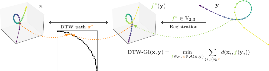
Figure 1: DTW-GI aligns time series by optimizing on temporal alignment $\pi$ (through Dynamic Time Warping) and feature space transformation $f$ (e.g. here in the Stiefel manifold $\mathbb{V}_{2,3}$). In the figure $\pi^{*},f^{*}$ denote the solutions of the optimization problem DTW-GI. Time series represented here are color-coded trajectories, whose starting (resp. end) point is depicted in blue (resp. yellow).

1 Introduction

Time series are subject to a number of variabilities that make their processing difficult in practice. One of the most well-known example is the temporal shift, usually handled using the celebrated Dynamic Time Warping (DTW, Sakoe & Chiba 1978) that aligns, in time, two time series and is invariant to any monotonically increasing temporal map. It has been initially introduced for speech processing applications and is now widely used in a variety of contexts such as human activity recognition (Chang et al., 2019), satellite image analysis (Wegner Maus et al., 2019) or medical applications (Huang & Lu, 2020; Janati et al., 2020).

Another source of variability in time series is feature space alterations, that may occur due to a permutation of sensors, changes in sensor properties or even different number of sensors. This problem of heterogeneous representations, also called distribution shifts in machine learning, has been studied mostly on non-structured data. It has been shown that algorithms are notoriously weak (Ben-David et al., 2010) when it comes to generalizing to out-of-distribution samples, as they rely on the correlations that are found in the training data (Arjovsky et al., 2019). Consequently, dedicated paradigms such as domain adaptation (Kouw & Loog, 2019) directly take into account this problem in the learning process. Another approach is to learn with respect to some invariance classes (based on some prior knowledge) in order to be more robust to irrelevant feature transformations (Battaglia et al., 2018; Goodfellow et al., 2009). In this work, we aim at tackling this problem in the time series context through the definition of similarity measures that naturally encode desirable invariances. More precisely, we introduce similarity measures that are able to deal with both temporal and feature space transformations.

There exist many frameworks to register different spaces under some classes of invariance. In the shape analysis community, matching objects under rigid transformations is a widely studied problem. Iterative Closest Point (ICP, Chen & Medioni 1992) is a standard algorithm for such a task. It acts by alternating two simple steps: (i) matching points using nearest neighbor search and (ii) registering shapes together based on the obtained matches, which is known as the orthogonal Procrustes problem that has a closed form solution (Goodall, 1991). This idea is further explored in Cohen & Guibas (1999); Alvarez-Melis et al. (2019), where optimal transport is used to match points in the first step, and a recent extension to objects with a hierarchical structure has been introduced in Alvarez-Melis et al. (2020) that considers a dedicated invariance class for the registration step.

This heterogeneous setting has also been investigated in the time series context, where the goal is to align series of features lying in different spaces. One of the most salient track of research in this setting is the Canonical Time Warping (CTW) method. CTW (Zhou & Torre, 2009) has been introduced for human motion alignment under rigid space transformations. It consists of temporal alignment (using DTW) of transformed time series, using Canonical Correlation Analysis (CCA) to define the feature space transform. Few extensions to CTW have been proposed. GTW (Zhou & De la Torre, 2012) parametrizes CTW temporal alignments in continuous time instead of relying on DTW. Deep CTW (Trigeorgis et al., 2016) extends CTW by learning a feature space embedding (in the form of a neural network) before performing CTW. Finally, Canonical soft Time Warping applies the CTW methodology to soft alignments (see Section 2 for more details on soft alignments). In the same vein as CTW, Deng et al. (2020) learns an invariant subspace based on DTW alignments. More recently, GromovDTW (Cohen et al., 2021) has been introduced as an extension of the Gromov-Wasserstein distance measure between heterogeneous distributions to the time series context. GromovDTW relies on time series self-similarities as a way to circumvent the need to compute distances across feature spaces. Compared to these approaches, our method works by optimizing a map between feature spaces, hence allowing one to (i) add prior information in the form of constraints on the set of allowed maps and (ii) use the computed map for downstream application, as illustrated in our experiments on MoCap data (as described in Section 4).

In more detail, we aim at tackling both temporal and feature space invariances. To do so, we state the problem as a joint optimization over temporal alignments and feature space transformations, as depicted in Figure 1. Our general framework allows the use of either DTW or its smoothed counterpart softDTW as an alignment procedure. Similarly, though rigid transformations of the feature space seem a reasonable invariance class, we show that our method can be used in conjunction with other families of transformations. Such a framework allows considering the case when time series differ both in length and feature space dimensionality. We introduce two different optimization procedures that could be used to tackle this problem and show experimentally that they lead to effectively invariant similarity measures. Our method can also be used to compute meaningful barycenters even when time series at stake do not lie in the same feature space. Finally, we showcase the versatility of our method and the importance of jointly learning feature space transformations and temporal alignments on two real-world applications that are time series forecasting for human motion and cover song identification.

2 Dynamic Time Warping (DTW)

Dynamic Time Warping (DTW, Sakoe & Chiba 1978) is an algorithm used to assess similarity between time series, with extensions to multivariate time series proposed in Ten Holt et al. (2007); Wöllmer et al. (2009). In its standard form, given two multivariate time series $\mathbf{x}\in{\mathbb{R}}^{T_{x}\times p}$ and $\mathbf{y}\in\mathbb{R}^{T_{y}\times p}$ of the same dimensionality $p$, DTW is defined as:

$$\operatorname{DTW}(\mathbf{x},\mathbf{y})=\min_{\pi\in\mathcal{A(\mathbf{x},\mathbf{y})}}\sum_{(i,j)\in\pi}d(\mathbf{x}_{i},\mathbf{y}_{j})$$ (1)

where $\mathcal{A(\mathbf{x},\mathbf{y})}$ is the set of all admissible alignments between $\mathbf{x}$ and $\mathbf{y}$ and $d$ is a ground metric. In most cases, $d$ is the squared Euclidean distance, i.e. $d(\mathbf{x}_{i},\mathbf{y}_{j})=\|\mathbf{x}_{i}-\mathbf{y}_{j}\|^{2}$.

An alignment $\pi$ is a sequence of pairs of time frames which is considered to be admissible iff (i) it matches first (and respectively last) indexes of time series $\mathbf{x}$ and $\mathbf{y}$ together, (ii) it is monotonically increasing and (iii) it is connected (i.e. every index from one time series must be matched with at least one index from the other time series). Efficient computation of the above-defined similarity measure can be performed in quadratic time using dynamic programming, relying on the following recurrence formula:

$$\operatorname{DTW}(\mathbf{x}_{\rightarrow t_{1}},\mathbf{y}_{\rightarrow t_{2}})=d(\mathbf{x}_{t_{1}},\mathbf{y}_{t_{2}})+\min\left\{\begin{array}[]{l}\operatorname{DTW}(\mathbf{x}_{\rightarrow t_{1}},\mathbf{y}_{\rightarrow t_{2}-1})\\ \operatorname{DTW}(\mathbf{x}_{\rightarrow t_{1}-1},\mathbf{y}_{\rightarrow t_{2}})\\ \operatorname{DTW}(\mathbf{x}_{\rightarrow t_{1}-1},\mathbf{y}_{\rightarrow t_{2}-1})\end{array}\right.$$ (2)

where we denote by $\mathbf{x}_{\rightarrow t}$ the time series $\mathbf{x}$ observed up to time $t$. Many variants of this similarity measure have been introduced. For example, the set of admissible alignment paths can be restricted to those lying close to the diagonal using the so-called Itakura parallelogram or Sakoe-Chiba band, or a maximum path length can be enforced (Zhang et al., 2017). Most notably, a differentiable variant of DTW, coined softDTW, has been introduced in Cuturi & Blondel (2017) and is based on previous works on alignment kernels (Cuturi et al., 2007). It replaces the min operation in Equation 2 by a soft-min operator $\min^{\gamma}$ whose smoothness is controlled by a parameter $\gamma>0$, resulting in the $\text{DTW}_{\gamma}$ distance:

$$\text{DTW}_{\gamma}(\mathbf{x},\mathbf{y})=\operatorname*{\min{}^{\gamma}}_{\pi\in\mathcal{A(\mathbf{x},\mathbf{y})}}\sum_{(i,j)\in\pi}d(\mathbf{x}_{i},\mathbf{y}_{j})=-\gamma\log\left(\sum_{\pi\in\mathcal{A(\mathbf{x},\mathbf{y})}}e^{-\sum_{(i,j)\in\pi}d(\mathbf{x}_{i},\mathbf{y}_{j})/\gamma}\right).$$ (3)

In the limit case $\gamma=0$, $\min^{\gamma}$ reduces to a hard min operator and $\text{DTW}_{\gamma}$ is equivalent to the DTW algorithm.

3 DTW with Global Invariances

Despite their widespread use, DTW and softDTW are not able to deal with time series of different dimensionalities or to encode feature transformations that may arise between time series. In the following, we introduce a new similarity measure aiming at aligning time series in this complex setting and provide ways to compute associated alignments. We also derive a Fréchet mean formulation that allows computing barycenters under this new geometry.

3.1 Definitions

Let $\mathbf{x}\in\mathbb{R}^{T_{x}\times p_{x}}$ and $\mathbf{y}\in\mathbb{R}^{T_{y}\times p_{y}}$ be two time series of length $T_{x}$ and $T_{y}$. In the following, we assume that the dimension $p_{x}\geq p_{y}$. In order to allow comparison between time series $\mathbf{x}$ and $\mathbf{y}$, we optimize on a family of functions $\mathcal{F}$ that map $\mathbf{y}$ onto the feature space in which $\mathbf{x}$ lies. More formally, we define Dynamic Time Warping with Global Invariances (DTW-GI) as the solution of the following joint optimization problem:

$$\text{DTW-GI}(\mathbf{x},\mathbf{y})=\min_{f\in\mathcal{F},\pi\in\mathcal{A}(\mathbf{x},\mathbf{y})}\sum_{(i,j)\in\pi}d(\mathbf{x}_{i},f(\mathbf{y}_{j})),$$ (4)

where $\mathcal{F}$ is a family of functions from $\mathbb{R}^{p_{y}}$ to $\mathbb{R}^{p_{x}}$. Properties (including symmetry) of this similarity measure are detailed in Sec. 3.1.1. Note that this problem can also be written as:

$$\text{DTW-GI}(\mathbf{x},\mathbf{y})=\min_{f\in\mathcal{F},\pi\in\mathcal{A}(\mathbf{x},\mathbf{y})}\left\langle\mathbf{W}_{\pi},C(\mathbf{x},f(\mathbf{y}))\right\rangle$$ (5)

where $f(\mathbf{y})$ is a shortcut notation for the transformation $f$ applied to all observations in $\mathbf{y}$, $\left\langle.,.\right\rangle$ denotes the Frobenius inner product, $W_{\pi}$ is defined as:

$$\forall i\leq T_{x},j\leq T_{y},\,(\mathbf{W}_{\pi})_{i,j}=\begin{cases}1&\text{ if }(i,j)\in\pi\\ 0&\text{ otherwise}\\ \end{cases}$$ (6)

and $C(\mathbf{x},f(\mathbf{y}))$ is the cross-similarity matrix of squared Euclidean distances between samples from $\mathbf{x}$ and $f(\mathbf{y})$, respectively. This definition can be extended to the softDTW case of Equation 3 as proposed in the following:

$$\text{DTW}_{\gamma}\text{-GI}(\mathbf{x},\mathbf{y})= \min_{f\in\mathcal{F}}\operatorname*{\min{}^{\gamma}}_{\pi\in\mathcal{A}(\mathbf{x},\mathbf{y})}\left\langle\mathbf{W}_{\pi},C(\mathbf{x},f(\mathbf{y}))\right\rangle$$ (7)

$$= \min_{f\in\mathcal{F}}-\gamma\log\sum_{\pi\in\mathcal{A(\mathbf{x},\mathbf{y})}}e^{-\left\langle\mathbf{W}_{\pi},C(\mathbf{x},f(\mathbf{y}))\right\rangle/\gamma}.$$

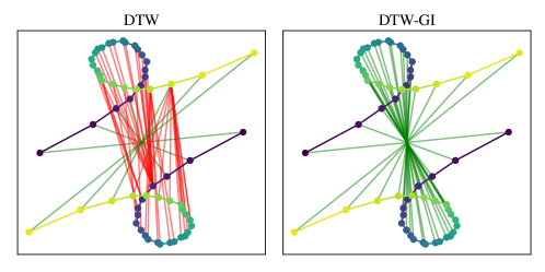
Figure 2: Example alignments between 2D time series (trajectories in the plane). Color coding corresponds to timestamps. Our DTW-GI method jointly estimates temporal alignment and global rotation between time series. On the contrary, standard DTW alignment fails at capturing feature space distortions and therefore produces a mostly erroneous alignment (matching in red), except at the beginning and end of the time series, whose alignments are preserved thanks to DTW border constraints (see Section 2).

Note that, due to the use of a soft-min operator, Equation 7 is no longer a joint optimization.

These similarity measures estimate both temporal alignment and feature space transformation between time series simultaneously, allowing the alignment of time series when the similarity should be defined up to a global transformation. For instance, one can see in Figure 2 two temporal alignments between two series in 2D that have been rotated in their feature space. In this case DTW-GI, whose invariant is the space of rotations, recovers the proper alignment whereas DTW fails.

3.1.1 Properties of DTW-GI

By definition, DTW-GI and softDTW-GI are invariant under any global transformation $T(\cdot)$ such that $\{f\circ T\,|\,f\in\mathcal{F}\}=\mathcal{F}$ (i.e. $\mathcal{F}$ is stable under $T$), which motivates the name (soft)DTW with Global Invariances. Moreover, DTW-GI inherits from some of the classical DTW properties. First, if for any $f\in\mathcal{F},f^{-1}$ exists and is in $\mathcal{F}$ (which implies $p_{x}=p_{y}$), and if elements of $\mathcal{F}$ are norm preserving operations, then DTW-GI and softDTW-GI are symmetric, since in this case:

$$\text{DTW-GI}(\mathbf{x},\mathbf{y}) = \min_{f\in\mathcal{F},\pi\in\mathcal{A}(\mathbf{x},\mathbf{y})}\sum_{(i,j)\in\pi}d(\mathbf{x}_{i},f(\mathbf{y}_{j}))$$ (8)

$$= \min_{f\in\mathcal{F},\pi\in\mathcal{A}(\mathbf{x},\mathbf{y})}\sum_{(i,j)\in\pi}d(f(f^{-1}(\mathbf{x}_{i})),f(\mathbf{y}_{j}))$$ (9)

$$= \min_{f\in\mathcal{F},\pi\in\mathcal{A}(\mathbf{x},\mathbf{y})}\sum_{(i,j)\in\pi}d(f^{-1}(\mathbf{x}_{i}),\mathbf{y}_{j})$$ (10)

$$= \min_{f\in\mathcal{F},\pi\in\mathcal{A}(\mathbf{x},\mathbf{y})}\sum_{(i,j)\in\pi}d(f(\mathbf{x}_{i}),\mathbf{y}_{j})$$ (11)

$$= \min_{f\in\mathcal{F},\pi\in\mathcal{A}(\mathbf{y},\mathbf{x})}\sum_{(i,j)\in\pi}d(\mathbf{y}_{i},f(\mathbf{x}_{j}))=\text{DTW-GI}(\mathbf{y},\mathbf{x}).$$ (12)

Though the constraints on $\mathcal{F}$ for this condition to hold might appear rather strong, this still allows to include standard rigid transformations such as rotations, translations and reflections.

Finally, it is straightforward to see that ${\text{DTW-GI}(\mathbf{x},\mathbf{x})=0}$ for any time series $\mathbf{x}$ as soon as $\mathcal{F}$ contains the identity map. More generally, regardless of the class of functions $\mathcal{F}$ and for any pair of time series $(\mathbf{x},\mathbf{y})$, we have ${\text{DTW-GI}(\mathbf{x},\mathbf{y})=0}$ iff there exists $f\in\mathcal{F}$ such that $\mathbf{x}$ and $f(\mathbf{y})$ are equal up to repetitions in the series.

3.2 Optimization

Optimization on the above-defined losses can be performed in several ways, depending of the nature of $\mathcal{F}$. We now present one optimization scheme for each loss.

3.2.1 Gradient descent

We first consider the optimization on the softDTW-GI loss (Equation 7) in the case where $\mathcal{F}$ is a parametric family of functions, here denoted $f_{\theta}$, that are differentiable with respect to their parameters $\theta$. The optimization can be done with a gradient descent on the parameters of $f_{\theta}$. Since softDTW is smooth (contrary to DTW), this strategy can be used to compute gradients of $\text{DTW}_{\gamma}\text{-GI}$ w.r.t. $\theta$.

Complexity for this approach is driven by (i) that of a softDTW computation and (ii) that of computing $f_{\theta}(\mathbf{y})$. If we denote the latter $c_{f}$, overall complexity for this approach is hence $O(n_{\text{iter}}(T_{x}T_{y}p_{x}+c_{f}))$. Note that when Riemannian optimization is involved, an extra complexity term has to be added, corresponding to the cost of projecting gradients onto the considered manifold. This cost is $O(p_{y}^{3})$ for example when optimization is performed on the Stiefel manifold (Wen & Yin, 2013), which is an important case for our applications, as discussed in more details in the following.

3.2.2 Block Coordinate Descent (BCD)

When DTW-GI (see Equation 5) is concerned, we introduce another strategy that consists in alternating minimization over (i) the temporal alignment and (ii) the feature space transformations. We will refer to this strategy as Block Coordinate Descent (BCD) in the following.

Optimization over the alignment path given a fixed transformation $f$ solely consists in a DTW alignment, as described in Section 2. For a fixed alignment path $\pi$, the optimization problem then becomes:

$$\min_{f\in\mathcal{F}}\left\langle\mathbf{W}_{\pi},C(\mathbf{x},f(\mathbf{y}))\right\rangle.$$ (13)

Recall that $C$ is a matrix of squared distances, which means that the problem above is a weighted least square problem. Depending on $\mathcal{F}$, there can exist a closed form solution for this problem (e.g. when $\mathcal{F}$ is the set of affine maps with no further constraints). Let us first note that the matrix $C$ can be rewritten as:

$$C(\mathbf{x},f(\mathbf{y}))=\mathbf{u}_{\mathbf{x}}{\mathbf{1}}_{T_{y}}^{\top}+{\mathbf{1}}_{T_{x}}\mathbf{v}_{f,\mathbf{y}}^{\top}-2\mathbf{x}f(\mathbf{y})^{\top}$$ (14)

where:

$$\mathbf{u}_{\mathbf{x}}=(\|\mathbf{x}_{1}\|^{2},\dots,\|\mathbf{x}_{T_{x}}\|^{2})^{\top}\text{ and }{\mathbf{v}_{f,\mathbf{y}}=(\|f(\mathbf{y}_{1})\|^{2},\dots,\|f(\mathbf{y}_{T_{y}})\|^{2})^{\top}}\,\,$$

and ${\mathbf{1}}_{n}=(\underbrace{1,\cdots,1}_{n\text{ times}})^{\top}$. In particular, the optimization problem (13) reduces to maximizing $\left\langle\mathbf{W}_{\pi},\mathbf{x}f(\mathbf{y})^{\top}\right\rangle$ when $\mathcal{F}$ is a set of norm preserving operations.

3.2.3 Estimating $f$ in the Stiefel manifold

Let us consider the special case where $\mathcal{F}$ is the set of linear maps whose linear operator is an orthonormal matrix, hence lying on the Stiefel manifold that we denote $\mathbb{V}_{p_{y},p_{x}}$ in the following. It is defined for $p_{y}\leq p_{x}$ as $\mathbb{V}_{p_{y},p_{x}}=\{\mathbf{P}\in\mathbb{R}^{p_{x}\times p_{y}},\mathbf{P}^{\top}\mathbf{P}=\mathbf{I}_{p_{y}}\}$ and this invariance class encodes rigid transformations of the features. In this case, the optimization problem becomes:

$$\min_{\mathbf{P}\in\mathbb{V}_{p_{y},p_{x}}}\left\langle\mathbf{W}_{\pi},\mathbf{u}_{\mathbf{x}}{\mathbf{1}}_{T_{y}}^{\top}+{\mathbf{1}}_{T_{x}}\mathbf{v}_{\mathbf{P},\mathbf{y}}^{\top}-2\mathbf{x}\mathbf{P}\mathbf{y}^{\top}\right\rangle$$ (15)

and we have $\mathbf{v}_{\mathbf{P},\mathbf{y}}=(\|\mathbf{P}\mathbf{y}_{1}\|^{2},\dots,\|\mathbf{P}\mathbf{y}_{T_{y}}\|^{2})^{\top}=(\|\mathbf{y}_{1}\|^{2},\dots,\|\mathbf{y}_{T_{y}}\|^{2})^{\top}=\mathbf{v}_{\mathbf{y}}$ since for all $j,\|\mathbf{P}\mathbf{y}_{j}\|^{2}=\mathbf{y}_{j}^{\top}\mathbf{P}^{\top}\mathbf{P}\mathbf{y}_{j}=\|\mathbf{y}_{j}\|^{2}$ and thus the considered applications are norm-preserving. Overall, we get the following optimization problem:

$$\min_{\mathbf{P}\in\mathbb{V}_{p_{y},p_{x}}}\left\langle\mathbf{W}_{\pi},\mathbf{u}_{\mathbf{x}}{\mathbf{1}}_{T_{y}}^{\top}+{\mathbf{1}}_{T_{x}}\mathbf{v}_{\mathbf{y}}^{\top}\right\rangle-2\left\langle\mathbf{W}_{\pi},\mathbf{x}\mathbf{P}\mathbf{y}^{\top}\right\rangle$$ (16)

which, since the term $\left\langle\mathbf{W}_{\pi},\mathbf{u}_{\mathbf{x}}{\mathbf{1}}_{T_{y}}^{\top}+{\mathbf{1}}_{T_{x}}\mathbf{v}_{\mathbf{y}}^{\top}\right\rangle$ does not depend on $\mathbf{P}$, is equivalent to solving:

$$\max_{\mathbf{P}\in\mathbb{V}_{p_{y},p_{x}}}\left\langle\mathbf{W}_{\pi},\mathbf{x}\mathbf{P}\mathbf{y}^{\top}\right\rangle=\max_{\mathbf{P}\in\mathbb{V}_{p_{y},p_{x}}}\left\langle\mathbf{x}^{\top}\mathbf{W}_{\pi}\mathbf{y},\mathbf{P}\right\rangle$$ (17)

the last equality being a direct consequence of the cyclic property of the trace.

$\mathbf{P}\leftarrow\mathbf{I}_{p_{x},p_{y}}$;

repeat

       $\mathbf{W}_{\pi}\leftarrow$ Alignment matrix from $\operatorname{DTW}(\mathbf{x},\mathbf{yP}^{\top})$ ;

       $\mathbf{M}\leftarrow\mathbf{x}^{\top}\mathbf{W}_{\pi}\mathbf{y}$ (see Equation 17) ;

       $\mathbf{U},\bm{\Sigma},\mathbf{V}^{\top}\leftarrow\operatorname{SVD}(\mathbf{M})$ ;

       $\mathbf{P}\leftarrow\mathbf{U}\mathbf{V}^{\top}$ ;

      

until convergence;

Algorithm 1 Block-Coordinate Descent for DTW-GI with Stiefel registration

As described in Jaggi (2013), the latter problem can be solved exactly using Singular Value Decomposition (SVD): if $\mathbf{U}\bm{\Sigma}\mathbf{V}^{\top}=\mathbf{M}$ is the SVD of a matrix $\mathbf{M}$ of shape $(p_{y},p_{x})$, then $\mathbf{S}^{\star}=\mathbf{UV}^{\top}$ is a solution to the linear problem $\max_{\mathbf{S}\in\mathbb{V}_{p_{y},p_{x}}}\langle\mathbf{S},\mathbf{M}\rangle$. Note that this method can also tackle the case where $\mathcal{F}$ is an affine map whose linear part lies in the Stiefel manifold by realigning time series means, as discussed for example in Lawrence et al. (2019). A sketch of the algorithm is presented in Algorithm 1 (for the simplified case where time series means do not have to be realigned).

Interestingly, this optimization strategy where we alternate between time series alignment, i.e. time correspondences between both time series, and feature space transform optimization can be seen as a variant of the Iterative Closest Point (ICP) method in image registration (Chen & Medioni, 1992), in which nearest neighbors are replaced by matches resulting from DTW alignment. Its overall complexity is then $O(n_{\text{iter}}(T_{x}T_{y}p_{x}+p_{x}p_{y}^{2}))$. This complexity is equal to that of the gradient-descent when $p_{x}=O(p_{y})$. However, in practice, the number of iterations required is much lower for this BCD variant, making it a very competitive optimization scheme, as discussed in Section 4.

Generalizations.

The algorithms presented above are mainly focused on optimization on the Stiefel manifold. Note however that they are not strictly restricted to this case. Typically, (projected) gradient descent based optimization could be performed for softDTW-GI on any family of functions parametrized by a neural network. Regarding the BCD algorithm, it requires a numerically efficient way to compute the optimal feature space transform for a fixed alignment. In our experiment, we illustrate this in the context of cover song identification, for which aligning song keys is a well-known registration step (see Section 4.5 for details). Another example is for block-structured linear transformations of the features. More precisely, this corresponds to the case where the features are structured into $k$ groups i.e. $p_{x}=k\cdot q_{x}$ and $p_{y}=k\cdot q_{y}$ with $q_{y}\leq q_{x},k\in\mathbb{N}$ and when one looks for a linear transformation $\mathbf{p}\in\mathbb{R}^{q_{x}\times q_{y}}$ that aligns the features of each group. To make the connection with our framework, this coincides with a global transformation $\mathbf{P}\in\mathbb{R}^{p_{x}\times p_{y}}$ that can be written as $\mathbf{P}=\operatorname{blockdiag}_{k}({\mathbf{p}})$ where:

$$\operatorname{blockdiag}_{k}({\mathbf{p}})=\operatorname{diag}(\underbrace{{\mathbf{p}},\cdots,{\mathbf{p}}}_{k\text{ times }})=\begin{pmatrix}{\mathbf{p}}&\mathbf{0}&\dots&\mathbf{0}\\ \mathbf{0}&{\mathbf{p}}&\dots&\mathbf{0}\\ \vdots&\vdots&\ddots&\vdots\\ \mathbf{0}&\mathbf{0}&\dots&{\mathbf{p}}\end{pmatrix}.$$

In the special case of ${\mathbf{p}}\in\mathbb{V}_{q_{y},q_{x}}$ it is easy to show that ${\mathbf{P}}^{\top}{\mathbf{P}}=\mathbf{I}_{p_{y}}$ and thus ${\mathbf{P}}\in\mathbb{V}_{p_{y},p_{x}}$ which also corresponds to a rigid transform of the features but this time structured in blocks. In this situation, the alignment problem becomes:

$$\min_{\begin{smallmatrix}\mathbf{P}=\operatorname{blockdiag}_{k}({\mathbf{p}})\\ \text{ s.t. }{\mathbf{p}}\in\mathbb{V}_{q_{y},q_{x}}\end{smallmatrix}}\left\langle\mathbf{W}_{\pi},\mathbf{u}_{\mathbf{x}}{\mathbf{1}}_{T_{y}}^{\top}+{\mathbf{1}}_{T_{x}}\mathbf{v}_{\mathbf{P},\mathbf{y}}^{\top}-2\mathbf{x}\mathbf{P}\mathbf{y}^{\top}\right\rangle.$$ (18)

As ${\mathbf{P}}\in\mathbb{V}_{p_{y},p_{x}}$ we can use the same reasoning as above and show that it is equivalent to $\max_{{\mathbf{p}}\in\mathbb{V}_{q_{y},q_{x}}}\left\langle\mathbf{x}^{\top}\mathbf{W}_{\pi}\mathbf{y},\operatorname{blockdiag}_{k}({\mathbf{p}})\right\rangle$. Interestingly the latter problem also admits a closed form expression. More precisely by decomposing $\mathbf{x}^{\top}\mathbf{W}_{\pi}\mathbf{y}$ into $k$ blocks $\mathbf{C}_{ij}$, each of size $q_{x}\times q_{y}$, the solution is given by $\mathbf{S}^{\star}=\mathbf{U}\mathbf{V}^{\top}$ where $\mathbf{U},\mathbf{V}$ come from the SVD of $\sum_{i=1}^{k}\mathbf{C}_{ii}$, i.e. the sum of the diagonal blocks. For more details we refer the reader to the Lemma 6.1 in the supplementary materials. We will illustrate this type of transformation for the alignment of human motion trajectories in Section 4.4.

3.3 Barycenters

Let us now assume we are given a set $\{\mathbf{x}^{(i)}\}_{i}$ of time series of possibly different lengths and dimensionalities. A barycenter of this set in the DTW-GI sense is a solution to the following optimization problem:

$$\min_{\mathbf{b}\in\mathbb{R}^{T\times p}}\sum_{i}w_{i}\min_{f_{i}\in\mathcal{F}}\operatorname{DTW}(\mathbf{x}^{(i)},f_{i}(\mathbf{b})),$$ (19)

where weights $\{w_{i}\}_{i}$ as well as barycenter length $T$ and dimensionality $p$ are provided as input to the problem. Note that, with this formulation, when $\mathcal{F}$ is the Stiefel manifold, $p$ is supposed to be lower or equal to the dimensionality of any time series in the set $\{\mathbf{x}^{(i)}\}_{i}$.

In terms of optimization, as for similarity estimation, two schemes can be used. First, softDTW-GI barycenters can be estimated through gradient descent (and when the set of series to be averaged is large, a stochastic variant relying on minibatches can easily be implemented). Second, when BCD is used for time series alignment, barycenters can be estimated using a similar approach as DTW Barycenter Averaging (DBA, Petitjean et al. 2011), that would consist in alternating between barycentric coordinate estimation and DTW-GI alignments.

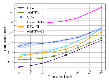
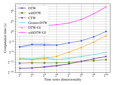
Figure 3: Computing time as a function of time series length (left) and dimensionality (right). Solid lines correspond to median values and shaded areas correspond to 20th (resp. 80th) percentiles.

4 Experiments

In this section, we provide an experimental study of DTW-GI (and its soft counterpart) on simulated data and real-world datasets. Unless otherwise specified, the set $\mathcal{F}$ of feature space transforms is the set of affine maps whose linear part lies in the Stiefel manifold. In all our experiments, tslearn (Tavenard et al., 2020) implementation is used for baseline methods and gradient descent on the Stiefel manifold is performed using GeoOpt (Kochurov et al., 2019; Becigneul & Ganea, 2019) in conjunction with PyTorch  (Paszke et al., 2019). Open source code of our method will be released upon publication.

4.1 Timings

We are first interested in a quantitative evaluation of the temporal complexity of our methods. Note that the theoretical complexity of DTW and softDTW are the same, hence any difference observed in this series of experiments between DTW-GI and softDTW-GI would be solely due to their optimization schemes discussed in Section 3.2. In these experiments, the number of iterations for BCD as well as the number of gradient steps for the gradient descent optimizer are set to 5,000. The BCD algorithm used for DTW-GI is stopped as soon as it reaches a local minimum, while early stopping is used for the gradient-descent variant with a patience parameter set to 100 iterations.

We first study the computation time as a function of the length of the time series involved. To do so, we generate random time series in dimension 8 and vary their lengths from 8 to 1,024 timestamps.

Figure 3 (left) shows a clear quadratic trend for all methods presented, except GromovDTW whose complexity is cubic w.r.t. the length of the time series due the tensor-matrix multiplication that is involved at each step of its pseudo-Frank-Wolfe algorithm (Cohen et al., 2021). Note that DTW-GI and its BCD optimizer clearly outperform the gradient descent strategy used for softDTW-GI because the latter requires more iterations before early stopping can be triggered. Building on this, we now turn our focus on the impact of feature space dimensionality $p$ (with a fixed time series length of 32). DTW and softDTW baselines are asymptotically linear with respect to $p$. Similarly, since GromovDTW relies on pre-computed self-similarity matrices, it only linearly depends in the feature space dimensionality for the computation of these self-similarity matrices. Since feature space registration is performed through optimization on the Stiefel manifold, both our optimization schemes rely on Singular Value Decomposition, which leads to an $O(p^{3})$ complexity that can also be observed for both methods in Figure 3 (right). Note also that the CTW baseline is slightly more computationally expensive than DTW-GI in practice, even if asymptotic complexities are the same as for DTW-GI.

4.2 Rotational invariance

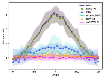
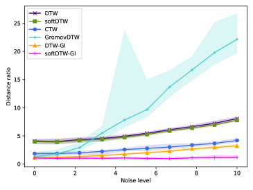
Figure 4: Illustration of the rotation invariance provided by DTW-GI. On the left, ratio of the distance to that of a non-rotated pair of spirals is presented as a function of the rotation angle for a fixed noise level. On the right, ratio of the distance to that of a non-rotated pair of spirals is presented as a function of the noise level for a fixed rotation angle $\pi$. Median distance ratios are reported as solid lines and shaded areas correspond to 20th (resp. 80th) percentiles.

We now evaluate the ability of our method to recover invariance to rotation. To do so, we rely on a synthetic dataset of noisy spiral-like 2D trajectories. For increasing values of an angle $\alpha$, we generate pairs of spirals rotated by $\alpha$ with additive Gaussian noise. Alignments between a reference time series and variants that are subject to an increasing rotation are computed and repeated 50 times per angle. The ratio of each distance to the distance when $\alpha=0$ is reported in Figure 4 (left). One can clearly see that the GI counterparts of DTW and softDTW are invariant to rotation in the 2d feature space, while DTW and softDTW are not. Interestingly, CTW and GromovDTW, that should be invariant to rotation, still exhibit an increase in the loss with the angle $\alpha$, suggesting that their algorithm has more difficulties reaching a global minimum in practice. Also, when varying the noise level in Figure 4 (right), one can notice that (soft-)DTW-GI are slightly more robust to high levels of noise than the CTW baseline, while GromovDTW is very sensitive to this noise level (the GW loss is a quadratic function of its input).

4.3 Barycenter computation

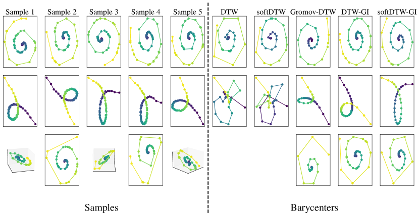
Figure 5: Barycenter computation using (i) DTW and softDTW baseline approaches, (ii) the alternative Gromov-DTW (Cohen et al., 2021) and (iii) our proposed rotation-invariant DTW-GI and softDTW-GI. Each row correspond to a different dataset, and the latter one contains both 2D and 3D trajectories, hence cannot be tackled by DTW nor softDTW. Trajectories are color-coded from blue (beginning of the series) to yellow (end of the series).

So as to better grasp the notion of similarity captured by our methods, we compute barycenters using the strategy presented in Section 3.3. Barycenters are computed for 3 different datasets: the first two are made of 2D trajectories of rotated and noisy spirals or folia, and the third one is composed of both 2- and 3-dimensional spirals (see samples in the left part of Figure 5). For each dataset, we provide barycenters obtained by three baseline methods. DTW Barycenter Averaging (DBA, Petitjean et al. 2011) is used for DTW while softDTW resorts to a gradient-descent scheme to compute the barycenters. Their GI counterpart use the same algorithms but rely on the alignments obtained from DTW-GI and softDTW-GI respectively. Finally, GromovDTW is optimized by alternating between computation of the barycenter self-similarity matrix and alignments, as done in Cohen et al. (2021). Note that the DTW and softDTW baselines cannot be used for the third dataset since features of the time series do not lie in the same ambient space. We would like to emphasize that the barycenter based on GromovDTW only finds a pairwise distance matrix from which the positions of the points must be inferred, for example by applying multidimensional scaling (MDS) (Kruskal & Wish, 1978) (as done here and in Cohen et al. 2021).

For the 2d spiral dataset, all the reconstructed barycenters can be considered as meaningful. Note however that the outer loop of the spiral (the one that suffers the most from the rotation) is better reconstructed using DTW-GI and softDTW-GI variants. When it comes to the folia trajectories, that are more impacted by rotations, baseline barycenters fail to capture the inherent structure of the trajectories at stake, while both our methods generate smooth and representative barycenters. DTW-GI and softDTW-GI are even able to recover barycenters when datasets are made of series that do not lie in the same space, as shown in the third row of Figure 5. Finally, in all three settings considered, temporal alignments successfully capture the irregular sampling from the samples to be averaged (denser towards the center of the spiral / loop of the folium).

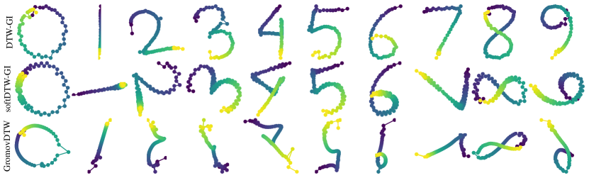
Figure 6: Barycenters computed on the RTD Dataset from 50 sample trajectories from each of the 10 classes using DTW-GI, softDTW-GI and GromovDTW. Trajectories are color-coded from blue (beginning of the series) to yellow (end of the series).

The RealSense based Trajectory Digit (RTD) dataset Alam et al. (2020) is made of digit writing trajectories. In our experiment, we have randomly sampled 50 trajectories per digit class and computed trajectory barycenters using (soft)DTW-GI and GromovDTW. On such data, expected invariants are rotations and translations. One can observe that invariance to mirroring strongly impacts GromovDTW’s barycenter estimation on classes 4, 7 and 9. On the other hand, for both DTW-GI and softDTW-GI, we obtain meaningful barycenters that do not suffer from mirroring artifacts and better preserve overall trajectories.

4.4 Time series forecasting

       

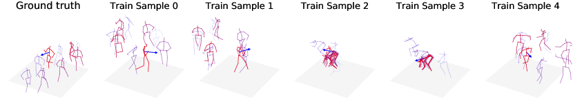
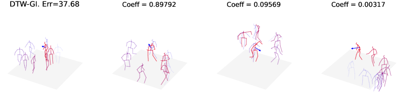
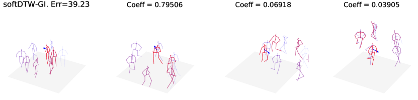
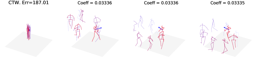
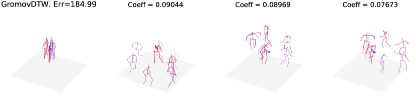
Figure 7: Examples of the forecasted subseries. (first row) The first sample is the ground-truth $\hat{\mathbf{y}}_{T^{\prime}\rightarrow}{}$ for the subject $S1$ and then training samples $\mathbf{x}^{(i)}_{T^{\prime}\rightarrow}{}$ are depicted. (from second to last row) Predictions for the methods DTW-GI, softDTW-GI, CTW and GromovDTW (the other methods are given in 8). In the first column the prediction $\hat{\mathbf{y}}_{T^{\prime}\rightarrow}{}$ is depicted along with the error $\|\hat{\mathbf{y}}_{T^{\prime}\rightarrow}{}-\mathbf{y}_{T^{\prime}\rightarrow}{}\|_{2}$. In the other columns, we illustrate the first $3$ neighbors w.r.t. the method $\mathbf{x}^{(i)}_{\rightarrow T^{\prime}}{}$ associated with their coefficients $a_{d}\left(\mathbf{y}_{\rightarrow T^{\prime}}{},\mathbf{x}^{(i)}_{\rightarrow T^{\prime}}{}\right)$. For each movement an arrow indicates the orientation of the subject. The beginning of the movement is displayed in shaded blue while the end is displayed in bold red.

       

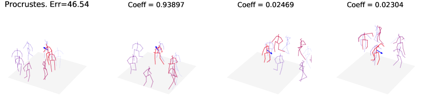
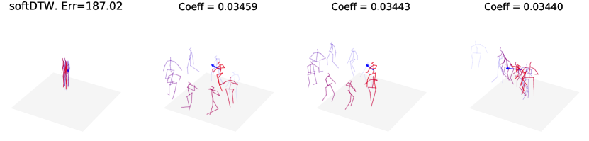
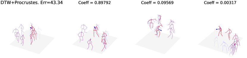
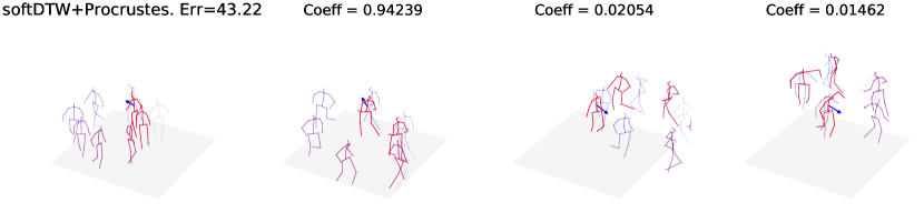
Figure 8: Examples of the forecasted subseries for the methods L2, L2+Procrustes, softDTW, DTW+Procrustes and softDTW+Procrustes

To further illustrate the benefit of our approach, we consider a time series forecasting problem (Le Guen & Thome, 2019), where the goal is to infer the future of a partially observed time series. In this setting, we suppose that we have access to a training set of full time series $\mathbf{X}$, with $\mathbf{x}^{(i)}\in\mathbf{X}$ a time series of length $T$ and dimensionality $p_{x}$, and another test set of partial time series $\mathbf{Y}$ where each $\mathbf{y}\in\mathbf{Y}$ is of length $T^{\prime}<T$ and dimensionality $p_{y}$. The goal is to predict the values for timestamps $T^{\prime}$ to $T$ for each test time series. We will denote by $\mathbf{x}_{\rightarrow T^{\prime}}$ the beginning of the time series $\mathbf{x}$ (up to time $T^{\prime}$) and $\mathbf{x}_{T^{\prime}\rightarrow}$ its end (from time $T^{\prime}$ to time $T$).

Let $d(\mathbf{y},\mathbf{x}^{(i)})$ denote a dissimilarity measure between time series $\mathbf{y}$ and $\mathbf{x}^{(i)}$ associated with a transformation $f_{i}\in\mathcal{F}:\mathbb{R}^{p_{x}}\rightarrow\mathbb{R}^{p_{y}}$ that maps the features of $\mathbf{x}^{(i)}$ onto the features of $\mathbf{y}$. This function aims at capturing the desired invariances in the feature space, as described in the previous section. A typical example is when $d$ is the (soft)DTW-GI cost, then the $f_{i}$ are the Stiefel linear maps which capture the possible rigid transformation between the features. We propose to predict the future of a time series $\mathbf{y}$ as follows:

$$\hat{\mathbf{y}}_{T^{\prime}\rightarrow}{}=\sum_{i}a_{d}\left(\mathbf{y}_{\rightarrow T^{\prime}}{},\mathbf{x}^{(i)}_{\rightarrow T^{\prime}}{}\right)f_{i}\left(\mathbf{x}^{(i)}_{T^{\prime}\rightarrow}{}\right)$$ (20)

where $a_{d}$ is the attention kernel:

$$a_{d}(\mathbf{y},\mathbf{x}_{i})=\frac{e^{-\lambda d(\mathbf{y},\mathbf{x}_{i})}}{\sum_{j}e^{-\lambda d(\mathbf{y},\mathbf{x}_{j})}}$$ (21)

with $\lambda>0$. The prediction is based on the known timestamps for the time series of the training set and on transformations $f_{i}$ that aim at capturing the latent transformation between training and test time series. The attention kernel gives more importance to time series that are close to the time series we want to forecast w.r.t. the notion of dissimilarity $d$. Note that for large values of $\lambda$, the softmax in Equation 21 converges to a hard max and the proposed approach corresponds to a nearest neighbor imputation.

4.4.1 Dataset and methodology

We use the Human3.6M dataset (Ionescu et al., 2014) which consists of 3.6 million video frames of human movements recorded in a controlled indoor motion capture setting. This dataset is composed of 7 actors performing 15 activities (“Walking”, “Sitting” …) twice. We are interested in forecasting the 3D positions of the subject joints evolving over time. More precisely, each data point $\mathbf{x}^{(i)}$ is a time series representing a skeleton of $32$ joints where each joint is described by 3D coordinates. This problem corresponds to $p_{x}=p_{y}=32\times 3$. We follow the same data partition as Coskun et al. (2017): the training set has 5 subjects (S6, S7, S8, S9 and S11) and the remaining 2 subjects (S1 and S5) compose the test set. In our experiments, 1) we split the limit frames as follows: we keep the first $T^{\prime}=300$ timestamps to calculate the coefficient $a_{d}\left(\mathbf{y}_{\rightarrow T^{\prime}}{},\mathbf{x}^{(i)}_{\rightarrow T^{\prime}}{}\right)$ and the transformations $f_{i}$ 2) we find the hyperparameter $\lambda$ which gives the best prediction (w.r.t. the $\ell_{2}$ norm) for $t\in[T^{\prime},T_{0}]$ (where $T_{0}=400$) 3) the remaining times $[T_{0},T^{\prime}]$ are used for the test set. We set the last limit frame as $T^{\prime}=1100$ which corresponds to predicting $T^{\prime}-T_{0}=700$ timestamps, that is predicting $14$ seconds of motion given the initial $8$ seconds. To emulate possible changes in signal acquisition (e.g. rotations of the camera), we randomly rotate the train subjects w.r.t. the $z$-axis. We consider the movements of type “Walking”, “WalkDog” and “WalkTogether” for the training set and “Walking” for the test set. Top row of Figure 7 illustrates samples of movements $\mathbf{x}^{(i)}_{\rightarrow T^{\prime}}{}$ resulting from this procedure and the resulting dataset is provided as supplementary material.

4.4.2 Competing structured prediction methods

We look for global transformations of the features $f_{i}:\mathbb{R}^{32\times 3}\rightarrow\mathbb{R}^{32\times 3}$. In order to obtain coherent transformations for each joint of the skeleton, the $f_{i}$ are structured as $f_{i}=(\underbrace{g_{i},g_{i},\cdots,g_{i}}_{32\text{ times }})$ where $g_{i}:\mathbb{R}^{3}\rightarrow\mathbb{R}^{3}$. In other words, we consider that there is only one global 3D transformation that aligns all the joints of two time series (such as one rotation). We use DTW-GI and softDTW-GI as our similarity measures and the associated maps $f_{i}$ as described in Equation 5 and in Equation 7. We compute DTW-GI using the BCD procedure with block-structured rigid transformations of the features as in Equation 18 ($q_{x}=q_{x}=3,k=32$ in this context). We calculate softDTW-GI with automatic differentiation as described in Section 3.2. In this experiment we set $\gamma=0.05$ for the smoothness parameter. We compare these methods to 8 baselines, that correspond to different pairs of time series similarity measure and feature space invariances. The first two baselines, denoted L2 and softDTW, do not encode any feature space invariance and are based on $\ell_{2}$ and softDTW similarities respectively. We also consider a Procrustes baseline (Goodall, 1991) defined as:

$$d(\mathbf{y}_{\rightarrow T^{\prime}}{},\mathbf{x}^{(i)}_{\rightarrow T^{\prime}}{})=\min_{{\mathbf{P}},\mathbf{b}}\|(\mathbf{x}^{(i)}_{\rightarrow T^{\prime}}{}\mathbf{P}^{\top}+\mathbf{b})-\mathbf{y}_{\rightarrow T^{\prime}}{}\|_{2}^{2}$$ (22)

where ${\mathbf{P}}=\operatorname{blockdiag}_{32}(\mathbf{p})$ with ${\mathbf{p}}\in\mathbb{V}_{3,3}$ and $\mathbf{b}=(\overline{\mathbf{b}},\cdots,\overline{\mathbf{b}})$ with $\overline{\mathbf{b}}\in\mathbb{R}^{3}$. The corresponding transformation $f_{i}$ is the affine map based on the optimal $\mathbf{P}^{\star},\mathbf{b}^{\star}$ found by the previous problem. We denote this baseline L2+Procrustes. Two other baselines are computed by first registering series using the Procrustes procedure defined above and then using the similarity measure $d(\mathbf{y}_{\rightarrow T^{\prime}}{},\mathbf{x}^{(i)}_{\rightarrow T^{\prime}}{})=\operatorname{DTW}(\mathbf{y}_{\rightarrow T^{\prime}}{},\mathbf{x}^{(i)}_{\rightarrow T^{\prime}}{}\textbf{P}^{\star\top}+\mathbf{b}^{\star})$ and $d(\mathbf{y}_{\rightarrow T^{\prime}}{},\mathbf{x}^{(i)}_{\rightarrow T^{\prime}}{})=\operatorname{DTW}_{\gamma}(\mathbf{y}_{\rightarrow T^{\prime}}{},\mathbf{x}^{(i)}_{\rightarrow T^{\prime}}{}\textbf{P}^{\star\top}+\mathbf{b}^{\star})$. They are denoted respectively by DTW+Procrustes and softDTW+Procrustes. Finally, we also compare with GromovDTW (Cohen et al., 2021) and CTW (Zhou & Torre, 2009). Note that the methods L2, softDTW, GromovDTW and CTW do not provide a transformation of the features of $\mathbf{x}^{(i)}_{\rightarrow T^{\prime}}{}$ onto those of $\mathbf{y}_{\rightarrow T^{\prime}}{}$ and, as such, we set $f_{i}=\operatorname{id}$ for all of these methods.

4.4.3 Results

Method	Average test error
L2	183.11 ± 3.90
softDTW (Cuturi & Blondel, 2017)	183.12 ± 3.90
CTW (Zhou & Torre, 2009)	183.11 ± 3.90
GromovDTW (Cohen et al., 2021)	181.28 ± 3.71
L2+Procrustes	46.33 ± 0.21
DTW+Procrustes	43.31 ± 0.03
softDTW+Procrustes	43.90 ± 0.11
DTW-GI (ours)	38.05 ± 0.37
softDTW-GI (ours)	39.58 ± 0.34

Table 1: Average error on tests subjects for the time series forecasting on the Human3.6M dataset

Qualitative and quantitative results are provided in Figures 7, 8 and Table 1 respectively. We evaluate, for each test subject, the $\ell_{2}$ reconstruction loss $\|\mathbf{y}_{T^{\prime}\rightarrow}-\hat{\mathbf{y}}_{T^{\prime}\rightarrow}{}\|_{2}$ between the ground truth time series and its prediction. Table 1 displays the average loss on the test subjects based on the best hyperparameter found using the timestamps $[T_{0},T^{\prime}]$. Figures 7 and 8 present examples of reconstructed movements for the different methods on one test subject as well as the $3$ highest coefficients $a_{d}$ with the corresponding neighbors.

We observe from the quantitative study that softDTW, L2, CTW and GromovDTW lead to the worst reconstruction losses while L2+Procrustes, DTW+Procrustes, softDTW+Procrustes and DTW-GI, softDTW-GI lead to the best ones. The results for the first four methods can be explained by the fact that none of them can use an explicit spatial transformation of the feature $f_{i}$ for the prediction and thus only a simple weighted average of the time-series $\mathbf{x}^{(i)}_{T^{\prime}\rightarrow}{}$ is realized. This is illustrated for CTW, GromovDTW, softDTW and L2 in Figures 7 and 8, where we can see that the prediction tends to shrink. We can also see that DTW+Procrustes and softDTW+Procrustes are superior to a simple L2+Procrustes which highlights the importance of temporal realignment. More importantly, the performances of DTW-GI and softDTW-GI are also better than DTW+Procrustes, softDTW+Procrustes and L2+Procrustes which shows that our joint realignment of time and space has an advantage over a two-step procedure such as DTW+Procrustes, softDTW+Procrustes which first finds the feature transformation and then aligns series in time.

Moreover, one can observe qualitatively that GromovDTW and CTW seem to uniformly average all the different motions to compensate for the lack of reprojection $f_{i}$. On the contrary, by capturing the possible spatial variability, L2+Procrustes and softDTW+Procrustes perform reasonably well qualitatively but the predicted movement is slightly less accurate than the one of softDTW-GI. This is due to the fact that L2+Procrustes or softDTW+Procrustes mainly chooses the movement corresponding to the first nearest neighbor ($a_{d}[1]=0.94$) while softDTW-GI is able to average other dynamics ($a_{d}[1]=0.79$). It is somehow a natural conclusion since the optimal transformations found by the Procrustes analysis supposes a trivial one-to-one correspondence of the timestamps (i.e. $\mathbf{y}_{\rightarrow T^{\prime}}(t)$ corresponds to $\mathbf{x}^{(i)}_{\rightarrow T^{\prime}}{}(t)$ at the same time $t$) and do not consider the temporal shifts between them. In this way, the method L2+Procrustes leads to unrealistic transformations when the dynamics of movements are not the same. Note that the two-step procedure softDTW+Procrustes is only slightly more precise as the feature realignment is independent of the temporal realignment since both are not optimized jointly. On the opposite, softDTW-GI method leads to the best qualitative results, highlighting the benefits of our approach over methods that whether discard the temporal variability of the movements (L2+Procrustes) or its spatial variability (softDTW).

4.5 Cover song identification

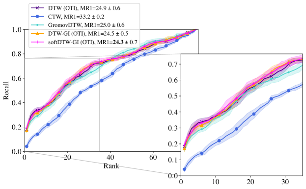
Figure 9: Cover song identification using the covers80 dataset. Methods are compared in terms of recall and results are averaged over 10 train / test set draws. For each method, the shaded area corresponds to one standard deviation around the mean value.

Cover song identification is the task of retrieving, for a given query song, its covers (i.e. different versions of the same song) in a training set. State-of-the-art methods either rely on anchor matches in the songs and/or on temporal alignments. In most related works, chroma or harmonic pitch class profile (HPCP) features are usually chosen, as they capture harmonic characteristics of the songs at stake (Heo et al., 2017).

For this experiment, we use the covers80 dataset (Ellis & Cotton, 2007) that consists in 80 cover pairs of pop songs and we evaluate the performance in terms of recall. Since the selection of features is not our main focus, we choose to extract chroma energy normalized statistics (CENS, (Müller et al., 2005)) over half a second windows. We compare variants of our method to a baseline that consists in a DTW alignment between songs transposed to the same key using the Optimal Transposition Index (OTI, (Serra et al., 2008)). This OTI computes a transposition based on average energy in each semitone band. For each competitor, test set songs are ranked based on their distances to query songs.

Figure 9 presents recall scores for compared methods as well as the mean rank of the first correctly identified cover (MR1) that is a standard evaluation metric for the task (used in MIREX for example). For the sake of readability, performance for DTW-GI with feature space optimization on the Stiefel manifold is omitted in this Figure. In practice, this approach leads to an MR1 of $29.0\pm 1.0$, which is clearly outperformed by the baseline relying on OTI. This is because a very common transformation in this setting is when cover songs are played in different keys, which is captured by the OTI transposition strategy. Similarly, CTW, which does not allow to use prior information about the form of the feature space registration into account, behaves poorly in this setting. Interestingly enough, the flexibility of our DTW-GI framework allows us to use the OTI strategy. Since the registration family $\mathcal{F}$ in this OTI setting is restricted to the set of 12 possible key transpositions, we do not rely on BCD in this case and rather seek for the exact optimum by computing (soft-)DTW for each of the 12 possible transpositions and retain the minimizer. This way, we are able to compute the optimal transposition index along the alignment path instead of computing it on averaged features, as the “DTW (OTI)” baseline does. This leads to a significant improvement of the performance for both DTW-GI and its soft counterpart and illustrates both the versatility of our method and the importance of performing joint feature space transformation and temporal alignment.

Note finally that the performance reached by the competitors in this study is far from what deep models can achieve. ByteCover Du et al. (2021), for example, reaches an MR1 of 3.54 on this task, by relying on both a triplet loss and a classification loss derived from a proxy classification task to train a ResNet. The use of softDTW-GI as an alternative similarity measure in the triplet loss of such an approach is left for future work.

5 Conclusion and Perspectives

We propose in this paper a novel similarity measure that can compare time series across different spaces in order to tackle both temporal and feature space invariances. This work extends the well-known Dynamic Time Warping algorithm to deal with time series from different spaces thanks to the introduction of a joint optimization over temporal alignments and space transformations. In addition, we provide a formulation for the computation of the barycenter of a set of times series under our new geometry, which is, to the best of our knowledge, the first barycenter formulation for a set of heterogeneous time series. Another important special case of our approach allows for performing temporal alignment of time series with invariance to rotations in the feature space.

We illustrate our approach on several datasets. First, we use simulated time series to study the computational complexity of our approach and illustrate invariance to rotations. Then, we apply our approach on two real-life datasets for human motion prediction and cover song identification where invariant similarity measures are shown to improve performance.

Extensions of this work will consider scenarios where features of the series do not lie in a Euclidean space, which would allow covering the case of structured data such as graphs evolving over time, for example. Future works also include the use of our methods in more elaborated models where, following ideas from Cai et al. (2019); Iwana et al. (2020), softDTW-GI could be used as a feature extractor in neural networks. It could also serve as a loss to train heterogeneous time series forecasting models (Le Guen & Thome, 2019; Cuturi & Blondel, 2017) or for imitation learning problems as considered in Cohen et al. (2021) where one wants to learn an agent (parametrized by a neural network) that generates trajectories on a different space than the initial ones.

Acknowledgments

This research was supported in part by ANR through the MATS project ANR-18-CE23-0006, by the AllegroAssai project ANR-19-CHIA-0009 and the ACADEMICS grant of the IDEXLYON, project of the Université de Lyon, PIA operated by ANR-16-IDEX-0005. NC is partially funded by the projects OTTOPIA ANR-20-CHIA-0030 AI chair. This research was also supported by 3rd Programme d’Investissements d’Avenir ANR-18-EUR-0006-02. This action benefited from the support of the Chair “Challenging Technology for Responsible Energy” led by l’X - Ecole polytechnique and the Fondation de l’Ecole polytechnique. TV gratefully acknowledges the support of the Centre Blaise Pascal’s IT test platform at ENS de Lyon (Lyon, France) for Machine Learning facilities. The platform operates the SIDUS solution (Quemener & Corvellec, 2013). The results are processed for visualizations using matplotlib (Hunter, 2007). Numerical computations involve numpy (Harris et al., 2020), scipy (Virtanen et al., 2020) and scikit-learn (Pedregosa et al., 2011) for the CTW implementation.

6 Appendix

For a matrix ${\mathbf{p}}$ we note:

$$\operatorname{blockdiag}_{k}({\mathbf{p}})=\operatorname{diag}(\underbrace{{\mathbf{p}},\cdots,{\mathbf{p}}}_{k\text{times}})=\begin{pmatrix}{\mathbf{p}}&\mathbf{0}&\dots&\mathbf{0}\\ \mathbf{0}&{\mathbf{p}}&\dots&\mathbf{0}\\ \vdots&\vdots&\ddots&\vdots\\ \mathbf{0}&\mathbf{0}&\dots&{\mathbf{p}}\end{pmatrix}$$

We will prove the following Lemma:

Lemma 6.1.

Let $q_{x},q_{y}\in\mathbb{N}$ such that $q_{y}\leq q_{x}$ and $k\in\mathbb{N}$. Consider ${\mathbf{C}}\in\mathbb{R}^{k\cdot q_{x}\times k\cdot q_{y}}$. We write the block diagonal decomposition of ${\mathbf{C}}$ as:

$${\mathbf{C}}=\begin{pmatrix}{\mathbf{C}}_{11}&{\mathbf{C}}_{12}&\dots&{\mathbf{C}}_{1k}\\ {\mathbf{C}}_{21}&{\mathbf{C}}_{22}&\dots&{\mathbf{C}}_{2k}\\ \vdots&\vdots&\ddots&\vdots\\ {\mathbf{C}}_{k1}&{\mathbf{C}}_{k2}&\dots&{\mathbf{C}}_{kk}\end{pmatrix}$$

where ${\mathbf{C}}_{ij}\in\mathbb{R}^{q_{x}\times q_{y}}$ for $i,j\in\{1,\cdots,k\}$. Consider $\overline{{\mathbf{C}}}=\sum_{i=1}^{k}{\mathbf{C}}_{ii}\in\mathbb{R}^{q_{x}\times q_{y}}$ the sum of the diagonal blocks of ${\mathbf{C}}$ and consider the full SVD decomposition of $\overline{{\mathbf{C}}}={\mathbf{U}}{\bm{\Sigma}}{\mathbf{V}}^{\top}$ where ${\mathbf{U}},{\bm{\Sigma}},{\mathbf{V}}\in\mathbb{R}^{q_{x}\times q_{y}}$. Then the solution to:

$$\underset{{\mathbf{p}}\in\mathbb{V}_{q_{y},q_{x}}}{\max}\ \langle{\mathbf{C}},\operatorname{blockdiag}_{k}({\mathbf{p}})\rangle$$ (23)

is given by ${\mathbf{p}}^{\star}={\mathbf{U}}{\mathbf{V}}^{\top}$.

Proof.

We have:

$$\begin{split}\langle{\mathbf{C}},\operatorname{blockdiag}_{k}({\mathbf{p}})\rangle_{F}&=\operatorname{tr}\left(\operatorname{blockdiag}_{k}({\mathbf{p}})^{\top}{\mathbf{C}}\right)=\operatorname{tr}\left(\begin{pmatrix}{\mathbf{p}}^{\top}&\mathbf{0}&\dots&\mathbf{0}\\ \mathbf{0}&{\mathbf{p}}^{\top}&\dots&\mathbf{0}\\ \vdots&\vdots&\ddots&\vdots\\ \mathbf{0}&\mathbf{0}&\dots&{\mathbf{p}}^{\top}\end{pmatrix}\begin{pmatrix}{\mathbf{C}}_{11}&{\mathbf{C}}_{12}&\dots&{\mathbf{C}}_{1k}\\ {\mathbf{C}}_{21}&{\mathbf{C}}_{22}&\dots&{\mathbf{C}}_{2k}\\ \vdots&\vdots&\ddots&\vdots\\ {\mathbf{C}}_{k1}&{\mathbf{C}}_{k2}&\dots&{\mathbf{C}}_{kk}\end{pmatrix}\right)\\ &=\operatorname{tr}\left(\begin{pmatrix}{\mathbf{p}}^{\top}{\mathbf{C}}_{11}&{\mathbf{p}}^{\top}{\mathbf{C}}_{12}&\dots&{\mathbf{p}}^{\top}{\mathbf{C}}_{1k}\\ {\mathbf{p}}^{\top}{\mathbf{C}}_{21}&{\mathbf{p}}^{\top}{\mathbf{C}}_{22}&\dots&{\mathbf{p}}^{\top}{\mathbf{C}}_{2k}\\ \vdots&\vdots&\ddots&\vdots\\ {\mathbf{p}}^{\top}{\mathbf{C}}_{k1}&{\mathbf{p}}^{\top}{\mathbf{C}}_{k2}&\dots&{\mathbf{p}}^{\top}{\mathbf{C}}_{kk}\end{pmatrix}\right)=\sum_{i=1}^{k}\operatorname{tr}({\mathbf{p}}^{\top}{\mathbf{C}}_{ii})\\ &=\operatorname{tr}\left({\mathbf{p}}^{\top}(\sum_{i=1}^{k}{\mathbf{C}}_{ii})\right)=\langle\sum_{i=1}^{k}{\mathbf{C}}_{ii},{\mathbf{p}}\rangle=\langle\overline{{\mathbf{C}}},{\mathbf{p}}\rangle\end{split}$$

Thus finding the solution to Equation 23 is the same as finding the solution to $\max_{{\mathbf{p}}\in\mathbb{V}_{q_{y},q_{x}}}\langle\overline{{\mathbf{C}}},{\mathbf{p}}\rangle$ which is given by the SVD of $\overline{{\mathbf{C}}}$ (Jaggi, 2013). ∎

References

- Alam et al. (2020) Md. Shahinur Alam, Ki-Chul Kwon, Md. Ashraful Alam, Mohammed Y. Abbass, Shariar Md Imtiaz, and Nam Kim. Trajectory-based air-writing recognition using deep neural network and depth sensor. Sensors, 20(2), 2020. ISSN 1424-8220.
- Alvarez-Melis et al. (2019) David Alvarez-Melis, Stefanie Jegelka, and Tommi S Jaakkola. Towards optimal transport with global invariances. In International Conference on Artificial Intelligence and Statistics, 2019.
- Alvarez-Melis et al. (2020) David Alvarez-Melis, Youssef Mroueh, and Tommi Jaakkola. Unsupervised hierarchy matching with optimal transport over hyperbolic spaces. In International Conference on Artificial Intelligence and Statistics, pp. 1606–1617. PMLR, 2020.
- Arjovsky et al. (2019) Martin Arjovsky, Léon Bottou, Ishaan Gulrajani, and David Lopez-Paz. Invariant risk minimization. arXiv preprint arXiv:1907.02893, 2019.
- Battaglia et al. (2018) Peter Battaglia, Jessica Blake Chandler Hamrick, Victor Bapst, Alvaro Sanchez, Vinicius Zambaldi, Mateusz Malinowski, Andrea Tacchetti, David Raposo, Adam Santoro, Ryan Faulkner, Caglar Gulcehre, Francis Song, Andy Ballard, Justin Gilmer, George E. Dahl, Ashish Vaswani, Kelsey Allen, Charles Nash, Victoria Jayne Langston, Chris Dyer, Nicolas Heess, Daan Wierstra, Pushmeet Kohli, Matt Botvinick, Oriol Vinyals, Yujia Li, and Razvan Pascanu. Relational inductive biases, deep learning, and graph networks. arXiv, 2018.
- Becigneul & Ganea (2019) Gary Becigneul and Octavian-Eugen Ganea. Riemannian adaptive optimization methods. In Proceedings of the International Conference on Learning Representations, 2019.
- Ben-David et al. (2010) Shai Ben-David, Tyler Lu, Teresa Luu, and Dávid Pál. Impossibility theorems for domain adaptation. In International Conference on Artificial Intelligence and Statistics, pp. 129–136, 2010.
- Cai et al. (2019) Xingyu Cai, Tingyang Xu, Jinfeng Yi, Junzhou Huang, and Sanguthevar Rajasekaran. Dtwnet: a dynamic time warping network. In Neural Information Processing Systems, pp. 11636–11646, 2019.
- Chang et al. (2019) Chien-Yi Chang, De-An Huang, Yanan Sui, Li Fei-Fei, and Juan Carlos Niebles. D3tw: Discriminative differentiable dynamic time warping for weakly supervised action alignment and segmentation. In IEEE Conference on Computer Vision and Pattern Recognition, pp. 3546–3555, 2019.
- Chen & Medioni (1992) Yang Chen and Gérard Medioni. Object modelling by registration of multiple range images. Image and Vision Computing, 10(3):145 – 155, 1992.
- Cohen et al. (2021) Samuel Cohen, Giulia Luise, Alexander Terenin, Brandon Amos, and Marc Peter Deisenroth. Aligning time series on incomparable spaces. In International Conference on Artificial Intelligence and Statistics, volume 130, pp. 1036–1044, 2021.
- Cohen & Guibas (1999) Scott Cohen and L Guibas. The Earth mover’s distance under transformation sets. In IEEE International Conference on Computer Vision, volume 2, pp. 1076–1083, 1999.
- Coskun et al. (2017) Huseyin Coskun, Felix Achilles, Robert DiPietro, Nassir Navab, and Federico Tombari. Long short-term memory kalman filters: Recurrent neural estimators for pose regularization. In International Conference on Computer Vision, Oct 2017.
- Cuturi & Blondel (2017) Marco Cuturi and Mathieu Blondel. Soft-DTW: a differentiable loss function for time-series. In International Conference on Machine Learning, pp. 894–903, 2017.
- Cuturi et al. (2007) Marco Cuturi, Jean-Philippe Vert, Oystein Birkenes, and Tomoko Matsui. A kernel for time series based on global alignments. In IEEE International Conference on Acoustics, Speech, and Signal Processing, volume 2, pp. II–413. IEEE, 2007.
- Deng et al. (2020) Huiqi Deng, Weifu Chen, Qi Shen, Andy J. Ma, Pong C. Yuen, and Guocan Feng. Invariant subspace learning for time series data based on dynamic time warping distance. Pattern Recognition, 102:107210, 2020.
- Du et al. (2021) Xingjian Du, Zhesong Yu, Bilei Zhu, Xiaoou Chen, and Zejun Ma. Bytecover: Cover song identification via multi-loss training. In IEEE International Conference on Acoustics, Speech, and Signal Processing, pp. 551–555, 2021. doi: 10.1109/ICASSP39728.2021.9414128.
- Ellis & Cotton (2007) Daniel PW Ellis and Courtenay Valentine Cotton. The 2007 labrosa cover song detection system, 2007.
- Goodall (1991) Colin Goodall. Procrustes methods in the statistical analysis of shape. Journal of the Royal Statistical Society: Series B (Methodological), 53(2):285–321, 1991.
- Goodfellow et al. (2009) Ian Goodfellow, Honglak Lee, Quoc V. Le, Andrew Saxe, and Andrew Y. Ng. Measuring invariances in deep networks. In Neural Information Processing Systems, pp. 646–654, 2009.
- Harris et al. (2020) Charles R Harris, K Jarrod Millman, Stéfan J Van Der Walt, Ralf Gommers, Pauli Virtanen, David Cournapeau, Eric Wieser, Julian Taylor, Sebastian Berg, Nathaniel J Smith, et al. Array programming with numpy. Nature, 585(7825):357–362, 2020.
- Heo et al. (2017) Hoon Heo, Hyunwoo J Kim, Wan Soo Kim, and Kyogu Lee. Cover song identification with metric learning using distance as a feature. In Proceedings of the International Society for Music Information Retrieval Conference, 2017.
- Huang & Lu (2020) Shih-Feng Huang and Hong-Ping Lu. Classification of temporal data using dynamic time warping and compressed learning. Biomedical Signal Processing and Control, 57:101781, 2020.
- Hunter (2007) John D Hunter. Matplotlib: A 2d graphics environment. Computing in science & engineering, 9(03):90–95, 2007.
- Ionescu et al. (2014) Catalin Ionescu, Dragos Papava, Vlad Olaru, and Cristian Sminchisescu. Human3.6m: Large scale datasets and predictive methods for 3d human sensing in natural environments. IEEE Transactions on Pattern Analysis and Machine Intelligence, 36(7):1325–1339, jul 2014.
- Iwana et al. (2020) Brian Kenji Iwana, Volkmar Frinken, and Seiichi Uchida. DTW-NN: a novel neural network for time series recognition using dynamic alignment between inputs and weights. Knowledge-Based Systems, 188, 1 2020. ISSN 0950-7051. doi: 10.1016/j.knosys.2019.104971.
- Jaggi (2013) Martin Jaggi. Revisiting Frank–Wolfe: Projection-free sparse convex optimization. In International Conference on Machine Learning, 2013.
- Janati et al. (2020) Hicham Janati, Marco Cuturi, and Alexandre Gramfort. Spatio-temporal alignments: Optimal transport through space and time. In International Conference on Artificial Intelligence and Statistics, pp. 1695–1704, 2020.
- Kochurov et al. (2019) Max Kochurov, Sergey Kozlukov, Rasul Karimov, and Viktor Yanush. Geoopt: Adaptive riemannian optimization in PyTorch, 2019. https://github.com/geoopt/geoopt.
- Kouw & Loog (2019) Wouter Marco Kouw and Marco Loog. A review of domain adaptation without target labels. IEEE Transactions on Pattern Analysis and Machine Intelligence, 2019.
- Kruskal & Wish (1978) J.B. Kruskal and M. Wish. Multidimensional Scaling. Sage Publications, 1978.
- Lawrence et al. (2019) Jim Lawrence, Javier Bernal, and Christoph Witzgall. A purely algebraic justification of the kabsch-umeyama algorithm. Journal of Research of the National Institute of Standards and Technology, 124:1–6, 2019.
- Le Guen & Thome (2019) Vincent Le Guen and Nicolas Thome. Shape and time distortion loss for training deep time series forecasting models supplementary material. In Neural Information Processing Systems, 2019.
- Müller et al. (2005) Meinard Müller, Frank Kurth, and Michael Clausen. Audio matching via chroma-based statistical features. In Proceedings of the International Society for Music Information Retrieval Conference, 2005.
- Paszke et al. (2019) Adam Paszke, Sam Gross, Francisco Massa, Adam Lerer, James Bradbury, Gregory Chanan, Trevor Killeen, Zeming Lin, Natalia Gimelshein, Luca Antiga, Alban Desmaison, Andreas Kopf, Edward Yang, Zachary DeVito, Martin Raison, Alykhan Tejani, Sasank Chilamkurthy, Benoit Steiner, Lu Fang, Junjie Bai, and Soumith Chintala. Pytorch: An imperative style, high-performance deep learning library. In H. Wallach, H. Larochelle, A. Beygelzimer, F. d’Alché Buc, E. Fox, and R. Garnett (eds.), Neural Information Processing Systems, pp. 8024–8035. 2019.
- Pedregosa et al. (2011) F. Pedregosa, G. Varoquaux, A. Gramfort, V. Michel, B. Thirion, O. Grisel, M. Blondel, P. Prettenhofer, R. Weiss, V. Dubourg, J. Vanderplas, A. Passos, D. Cournapeau, M. Brucher, M. Perrot, and E. Duchesnay. Scikit-learn: Machine learning in Python. Journal of Machine Learning Research, 12:2825–2830, 2011.
- Petitjean et al. (2011) François Petitjean, Alain Ketterlin, and Pierre Gançarski. A global averaging method for dynamic time warping, with applications to clustering. Pattern Recognition, 44(3):678 – 693, 2011.
- Quemener & Corvellec (2013) Emmanuel Quemener and Marianne Corvellec. Sidus—the solution for extreme deduplication of an operating system. Linux Journal, 2013(235):3, 2013.
- Sakoe & Chiba (1978) Hiroaki Sakoe and Seibi Chiba. Dynamic programming algorithm optimization for spoken word recognition. IEEE Transactions on Acoustics, Speech and Signal Processing, 26(1):43–49, 1978.
- Serra et al. (2008) Joan Serra, Emilia Gómez, and Perfecto Herrera. Transposing chroma representations to a common key. In Proceeding sof the IEEE Conference on The Use of Symbols to Represent Music and Multimedia Objects, pp. 45–48, 2008.
- Tavenard et al. (2020) Romain Tavenard, Johann Faouzi, Gilles Vandewiele, Felix Divo, Guillaume Androz, Chester Holtz, Marie Payne, Roman Yurchak, Marc Rußwurm, Kushal Kolar, et al. Tslearn, A Machine Learning Toolkit for Time Series Data. J. Mach. Learn. Res., 21(118):1–6, 2020.
- Ten Holt et al. (2007) Gineke A Ten Holt, Marcel JT Reinders, and EA Hendriks. Multi-dimensional dynamic time warping for gesture recognition. In Annual conference of the Advanced School for Computing and Imaging, volume 300, pp. 1, 2007.
- Trigeorgis et al. (2016) George Trigeorgis, Mihalis A Nicolaou, Stefanos Zafeiriou, and Bjorn W Schuller. Deep canonical time warping. In EEE Conference on Computer Vision and Pattern Recognition, pp. 5110–5118, 2016.
- Virtanen et al. (2020) Pauli Virtanen, Ralf Gommers, Travis E Oliphant, Matt Haberland, Tyler Reddy, David Cournapeau, Evgeni Burovski, Pearu Peterson, Warren Weckesser, Jonathan Bright, et al. Scipy 1.0: fundamental algorithms for scientific computing in python. Nature methods, 17(3):261–272, 2020.
- Wegner Maus et al. (2019) Victor Wegner Maus, Gilberto Câmara, Marius Appel, and Edzer Pebesma. dtwsat: Time-weighted dynamic time warping for satellite image time series analysis in R. Journal of Statistical Software, 88(5):1–31, 2019.
- Wen & Yin (2013) Zaiwen Wen and Wotao Yin. A feasible method for optimization with orthogonality constraints. Mathematical Programming, 142(1-2):397–434, 2013.
- Wöllmer et al. (2009) Martin Wöllmer, Marc Al-Hames, Florian Eyben, Björn Schuller, and Gerhard Rigoll. A multidimensional dynamic time warping algorithm for efficient multimodal fusion of asynchronous data streams. Neurocomputing, 73(1-3):366–380, 2009.
- Zhang et al. (2017) Zheng Zhang, Romain Tavenard, Adeline Bailly, Xiaotong Tang, Ping Tang, and Thomas Corpetti. Dynamic time warping under limited warping path length. Information Sciences, 393:91–107, 2017.
- Zhou & De la Torre (2012) Feng Zhou and Fernando De la Torre. Generalized time warping for multi-modal alignment of human motion. In IEEE Conference on Computer Vision and Pattern Recognition, pp. 1282–1289, 2012.
- Zhou & Torre (2009) Feng Zhou and Fernando Torre. Canonical time warping for alignment of human behavior. In Advances in neural information processing systems, pp. 2286–2294, 2009.