Fast and High-order Accuracy Numerical Methods for Time-Dependent Nonlocal Problems in $\mathbb{R}^{2}$

Abstract

In this paper, we study the Crank-Nicolson method for temporal dimension and the piecewise quadratic polynomial collocation method for spatial dimensions of time-dependent nonlocal problems. The new theoretical results of such discretization are that the proposed numerical method is unconditionally stable and its global truncation error is of $\mathcal{O}\left(\tau^{2}+h^{4-\gamma}\right)$ with $0<\gamma<1$, where $\tau$ and $h$ are the discretization sizes in the temporal and spatial dimensions respectively. Also we develop the conjugate gradient squared method to solving the resulting discretized nonsymmetric and indefinite systems arising from time-dependent nonlocal problems including two-dimensional cases. By using additive and multiplicative Cauchy kernels in non-local problems, structured coefficient matrix-vector multiplication can be performed efficiently in the conjugate gradient squared iteration. Numerical examples are given to illustrate our theoretical results and demonstrate that the computational cost of the proposed method is of $O(M\log M)$ operations where $M$ is the number of collocation points.

1 Introduction

In this paper, we study an error estimate and develop fast conjugate gradient squares method of the piecewise quadratic polynomial collocation (PQC) for time-dependent nonlocal problems, whose prototype is [1, 4, 14, 23]

($$* u_{t}(x,t)+\int_{\Omega}J(|x-y|)\left[u(x,t)-u(y,t)\right]dy=f(x,t),\quad(x,t)\in\Omega\times(0,T].$$)

Here $J(x)$ is a radial probability density with a nonnegative symmetric dispersal kernel, with nonhomogeneous Dirichlet boundary conditions and initial condition $u(x,0)=u_{0}(x)$. There are a lot of scientific phenomena that can be described by model ($*$) in various applications, for example, in materials science, biology, particle systems, image processing, coagulation models, mathematical finance, see [1, 4] for detailed discussion. The well-posedness (existence and uniqueness) of the model ($*$) can be found in the monograph [1, p. 46]. We notice that there are many different choices to prescribe $J(x)$ for nonlocal problems ($*$), e.g., the constant kernel, fractional Laplacian kernel or commonly used kernel [1, 10, 14, 29, 31]

$$J(x)\sim\frac{1}{x^{1+2s}},~{}~{}s\in[-0.5,1).$$

In this paper, we mainly focus on the case $s\in(-0.5,0)$, the other cases can be similarly studied. Then the nonlocal model ($*$) reduces to the following nonlocal diffusion problem

(1) $$\frac{\partial u(x,t)}{\partial t}+\int^{b}_{a}\frac{u(x)-u(y)}{|x-y|^{\gamma}}dy=f(x,t),\quad(x,t)\in(a,b)\times(0,T],\quad 0<\gamma<1.$$

To seek the numerical solution of time-dependent nonlocal problems, or specifically (1), we employ the piecewise quadratic polynomial collocation method to approximate the following weakly singular integral

$$I(a,b,x)=\int^{b}_{a}\frac{u(y)}{|x-y|^{\gamma}}dy,\quad x\in(a,b),\quad 0<\gamma<1,$$

in the discretization for non-local problems in (1.1). Note that the local truncation error with $\mathcal{O}\left(h^{3}\right)$ convergence was established in [2], where $h$ is the discretization size in the spatial dimension. The quasi-optimal error estimate with $\mathcal{O}\left(h^{4-\gamma}\right)$ convergence was provided in [16] or [3, p. 125]. By using the techniques of hypersingular integral [17, 18, 30], researchers provided an optimal error $\mathcal{O}\left(h^{4}\eta_{i}^{-\gamma}\right)$, $\eta_{i}=\min\left\{x_{i}-a,b-x_{i}\right\}$ for the weakly singular integral [11]. Numerical methods for the steady-state version of (1) have been proposed and studied in the literature. For example, the second-order convergence results are provided in [9, 29] by using the finite element method with piecewise linear polynomial basis. Recently, numerical results for the steady-state version of (1) with $\gamma=1$ was shown that the convergence rate is close to 1.5 by the PLC method [25]. There is still no theoretical convergence results for the PLC method. In [11], Chen et al. showed the optimal first order and third-order convergence rates for the PLC and the PQC methods respectively. To the best of our knowledge, there is only a few study for time-dependent nonlocal problems. In [13], Du et al. studied the two-dimensional nonlocal wave equation on unbounded domains and its numerical solution based on quadrature scheme.

The main aim of this paper is to study the Crank-Nicolson method for temporal dimension and the piecewise quadratic polynomial collocation method for spatial dimensions of time-dependent nonlocal problems in (1.1). The new theoretical results of such discretization are that the proposed numerical method is unconditionally stable and its global truncation error is of $\mathcal{O}\left(\tau^{2}+h^{4-\gamma}\right)$ with $0<\gamma<1$, where $\tau$ and $h$ are the discretization sizes in the temporal and spatial dimensions respectively. Also we employ the conjugate gradient squared method [22, 24] to solving the resulting discretized nonsymmetric and indefinite systems arising from time-dependent nonlocal problems. By using additive and multiplicative Cauchy kernels in non-local problems, structured coefficient matrix-vector multiplication [7, 19, 20, 28, 6, 15] can be performed efficiently in the conjugate gradient squared iteration. Numerical examples are given to illustrate our theoretical results and demonstrate that the computational cost of the proposed method is of $O(M\log M)$ operations where $M$ is the number of collocation points.

The paper is organized as follows. In Section 2, we provide the high-order scheme with the collocation method for solving nonlocal problems. In Section 3, the superconvergence rate with the Crank-Nicolson scheme is studied. In Section 4, we develop conjugate gradient squared method to solving the discretized linear system and discuss the computational cost and the storage requirement. In Section 5, experimental results are given to illustrate the effectiveness of the proposed numerical method. Finally, some concluding remarks are given in Section 6.

2 Discretization Schemes

In this section, we discuss about the discretization schemes of the nonlocal problems including two-dimensional cases.

2.1 One-dimensional Discretization

Review the piecewise quadratic polynomial collocation method and apply it to the following steady-state version of (1):

(2) $$\int^{b}_{a}\frac{u(x)-u(y)}{|x-y|^{\gamma}}dy=f(x),\quad 0<\gamma<1.$$

Let the mesh points $a=x_{0}<x_{\frac{1}{2}}<x_{1}<\cdots<x_{\frac{2M-1}{2}}<x_{M}=b$ be a partition with the uniform spatial stepsize $h=(b-a)/M$ and $0=t_{0}<t_{1}<\cdots<t_{N}=T$ with the time stepsize $\tau=T/N$. Denote $u_{i}^{k}$ as the approximated value of $u(x_{i},t_{k})$ and $f_{i}^{k+1/2}=f(x_{i},t_{k+1/2})$ with $t_{k+1/2}=\frac{t_{k}+t_{k+1}}{2}$.

Let the piecewise quadratic basis function $\phi_{i}(y)$ or $\phi_{i+\frac{1}{2}}(y)$ be given in [3, p. 499]. Then the piecewise Lagrange quadratic interpolant of $u(y)$ is

$$u_{Q}(y)=\sum^{M}_{i=0}u(x_{i})\phi_{i}(y)+\sum^{M-1}_{i=0}u\left(x_{i+\frac{1}{2}}\right)\phi_{i+\frac{1}{2}}(y).$$

According to (2.9) from [11], we can rewrite (2) as follows:

(3) $$\begin{split}\int^{b}_{a}\frac{u\left(x_{\frac{i}{2}}\right)-u_{Q}(y)}{\left|x_{\frac{i}{2}}-y\right|^{\gamma}}dy=f\left(x_{\frac{i}{2}}\right)+R_{\frac{i}{2}},\quad 1\leq i\leq 2M-1,\end{split}$$

with $R_{\frac{i}{2}}=\mathcal{O}\left(h^{4}\left(\eta_{\frac{i}{2}}\right)^{-\gamma}\right)$ and $\eta_{\frac{i}{2}}=\min\left\{x_{\frac{i}{2}}-a,b-x_{\frac{i}{2}}\right\}$ for $i=1,2,\cdots,2M-1$. Thus the discretization scheme of (3) is given by the following system:

$$\begin{split}&\left[d_{i}u_{i}-\sum^{M-1}_{j=1}m_{|i-j|}u_{j}-\sum^{M-1}_{j=0}q_{|i-j-\frac{1}{2}|-\frac{1}{2}}u_{j+\frac{1}{2}}\right]=f_{i}+\left(\beta_{i}u_{0}+\beta_{M-i}u_{M}\right),\\ &{\rm with}\ i=1,2,\cdots,M-1,\,{\rm and}\\ &\left[d_{i+\frac{1}{2}}u_{i+\frac{1}{2}}-\sum^{M-1}_{j=1}p_{|i+\frac{1}{2}-j|-\frac{1}{2}}u_{j}-\sum^{M-1}_{j=0}n_{|i-j|}u_{j+\frac{1}{2}}\right]=f_{i+\frac{1}{2}}+\left(\gamma_{i}u_{0}+\gamma_{M-i-1}u_{M}\right),\\ &{\rm with}\ i=0,1,2,\cdots,M-1.\end{split}$$

Here, the coefficients are given in (2.10) of [11]. For simplicity, we set $\eta_{h,\gamma}$ to be $\frac{h^{1-\gamma}}{(3-\gamma)(2-\gamma)(1-\gamma)}$ and explicitly compute $m_{0}=2(1+\gamma){\eta_{h,\gamma}}$, for $k\geq 1$,

$$m_{k}=4{\eta_{h,\gamma}}\left[(k+1)^{3-\gamma}\!-\!(k-1)^{3-\gamma}\right]\!-\!{\eta_{h,\gamma}}(3-\gamma)\left[(k+1)^{2-\gamma}+6k^{2-\gamma}+(k-1)^{2-\gamma}\right];$$

and $p_{0}=4{\eta_{h,\gamma}}\left[\left(\frac{3}{2}\right)^{3-\gamma}-\left(\frac{1}{2}\right)^{3-\gamma}\right]-{\eta_{h,\gamma}}(3-\gamma)\left[\left(\frac{3}{2}\right)^{2-\gamma}+3\left(\frac{1}{2}\right)^{2-\gamma}\right]$, for $k\geq 1$, $p_{k}=m_{k+\frac{1}{2}}$. Moreover $n_{0}={\eta_{h,\gamma}}{(2-\gamma)2^{\gamma+1}}$, $n_{k}=q_{k-\frac{1}{2}}$ for $k\geq 1$, and there exists

$$q_{k}=-8{\eta_{h,\gamma}}\left((k+1)^{3-\gamma}-k^{3-\gamma}\right)+4{\eta_{h,\gamma}}(3-\gamma)\left((k+1)^{2-\gamma}+k^{2-\gamma}\right),\,k\geq 0.$$

The boundary coefficients for $1\ \leq i\leq M-1$ are given by

$$\beta_{i}=4{\eta_{h,\gamma}}\left[i^{3-\gamma}\!-\!(i-1)^{3-\gamma}\right]-{\eta_{h,\gamma}}(3-\gamma)\left[3i^{2-\gamma}+\left(i-1\right)^{2-\gamma}-(2-\gamma)i^{1-\gamma}\right],$$

$\gamma_{i}=\beta_{i+\frac{1}{2}}$ and $\gamma_{0}={\eta_{h,\gamma}}{{(2-\gamma)(1-\gamma)}2^{\gamma-1}}$.

Using the matrix form of the grid functions

$$U=\left(u_{1},u_{2},\cdots,u_{M-1},u_{\frac{1}{2}},u_{\frac{3}{2}},\cdots,u_{M-\frac{1}{2}}\right)^{T}$$

and similarly for $F$. We can rewrite the above discretization scheme as follows:

(4) $$\begin{split}\mathcal{A}U=F+K~{}~{}{\rm with}~{}~{}\mathcal{A}=\left(\begin{matrix}\mathcal{D}_{1}&0\\ 0&\mathcal{D}_{2}\end{matrix}\right)-\left(\begin{matrix}\mathcal{M}&\mathcal{Q}\\ \mathcal{P}&\mathcal{N}\end{matrix}\right)=:{\cal D}-{\cal G},\end{split}$$

where the boundary data $K$ is given by

$$\begin{split}K&=\left(\eta_{1},\eta_{2},\cdots,\eta_{M-1},\eta_{\frac{1}{2}},\eta_{\frac{3}{2}},\cdots,\eta_{M-\frac{1}{2}}\right)^{T}u_{0}\\ &\quad+\left(\eta_{M-1},\eta_{M-2},\cdots,\eta_{1},\eta_{M-\frac{1}{2}},\eta_{M-\frac{3}{2}},\cdots,\eta_{\frac{1}{2}}\right)^{T}u_{M}.\end{split}$$

Moreover, $\mathcal{D}_{1}={\rm diag}\left(d_{1},d_{2},\ldots,d_{M-1}\right)$, $\mathcal{D}_{2}={\rm diag}\left(d_{\frac{1}{2}},d_{\frac{3}{2}},\ldots,d_{M-\frac{1}{2}}\right)$, and $\mathcal{M}={\rm toeplitz}\left(m_{0},m_{1},\ldots,m_{M-2}\right)$, $\mathcal{N}={\rm toeplitz}\left(n_{0},n_{1},\ldots,n_{M-1}\right)$. The rectangular matrices $\mathcal{P}$, $\mathcal{Q}$ are defined by

$$\begin{split}\mathcal{P}=\left[\begin{matrix}p_{0}&p_{1}&p_{2}&\cdots&p_{M-3}&p_{M-2}\\ p_{0}&p_{0}&p_{1}&\ddots&\ddots&p_{M-3}\\ p_{1}&p_{0}&p_{0}&\ddots&\ddots&\vdots\\ \vdots&\ddots&\ddots&\ddots&\ddots&p_{2}\\ p_{M-4}&\ddots&\ddots&\ddots&p_{0}&p_{1}\\ p_{M-3}&p_{M-4}&\ddots&p_{1}&p_{0}&p_{0}\\ p_{M-2}&p_{M-3}&p_{M-4}&\cdots&p_{1}&p_{0}\end{matrix}\right]_{M\times(M-1)}\end{split},$$

and

$$\begin{split}\mathcal{Q}=\left[\begin{matrix}q_{0}&q_{0}&q_{1}&\cdots&q_{M-4}&q_{M-3}&q_{M-2}\\ q_{1}&q_{0}&q_{0}&\ddots&\ddots&q_{M-4}&q_{M-3}\\ q_{2}&q_{1}&q_{0}&\ddots&\ddots&\ddots&q_{M-4}\\ \vdots&\ddots&\ddots&\ddots&\ddots&q_{1}&\vdots\\ q_{M-3}&\ddots&\ddots&\ddots&q_{0}&q_{0}&q_{1}\\ q_{M-2}&q_{M-3}&\cdots&q_{2}&q_{1}&q_{0}&q_{0}\end{matrix}\right]_{(M-1)\times M}\end{split}.$$

Hence, the full discretization of time-dependent non-local problems in (1.1) with Crank-Nicolson scheme is given by

(5) $$\left(I+\frac{\tau}{2}\mathcal{A}\right)U^{k}=\left(I-\frac{\tau}{2}\mathcal{A}\right)U^{k-1}+\tau F^{k-\frac{1}{2}}+\tau K^{k-\frac{1}{2}},\,k=1,2,\cdots,N,$$

with $U^{k}=\left(u^{k}_{1},u^{k}_{2},\cdots,u^{k}_{M-1},u^{k}_{\frac{1}{2}},u^{k}_{\frac{3}{2}},\cdots,u^{k}_{M-\frac{1}{2}}\right)^{T}$. Note that the local truncation error is of $\mathcal{O}\left(\tau^{2}+h^{4}\left(\eta_{\frac{i}{2}}\right)^{-\gamma}\right)$ with $\eta_{\frac{i}{2}}=\min\left\{x_{\frac{i}{2}}-a,b-x_{\frac{i}{2}}\right\}$.

2.2 Two-dimensional Nonlocal Problems with Multiplicative Cauchy Kernel

As one of the two-dimensional nonlocal problems, we consider the following nonlocal problem with multiplicative Cauchy kernel:

(6) $$\int_{\Omega}\frac{u(x,y)-u(\bar{x},\bar{y})}{|x-\bar{x}|^{\gamma}|y-\bar{y}|^{\gamma}}d\bar{x}d\bar{y}=f(x,y),\quad 0<\gamma<1,$$

with $\Omega=\left(a,b\right)\times\left(c,d\right)$. Taking the mesh points $a=x_{0}<x_{\frac{1}{2}}<x_{1}<\cdots<x_{\frac{2M_{x}-1}{2}}<x_{M_{x}}=b$ and $c=y_{0}<y_{\frac{1}{2}}<y_{1}<\cdots<y_{\frac{2M_{y}-1}{2}}<y_{M_{y}}=d$ as a partition with the uniform space stepsize $h_{x}=(b-a)/M_{x}$ in $x$ direction, and $h_{y}=(d-c)/M_{y}$ in $y$ direction, and $t_{k}=k\tau$ with the time stepsize $\tau=T/N$. Denote $u_{i,j}^{k}$ as the approximated value of $u\left(x_{i},y_{j},t_{k}\right)$ and $f_{i,j}^{k+1/2}=f\left(x_{i},y_{j},t_{k+1/2}\right)$ with $t_{k+1/2}=\frac{t_{k}+t_{k+1}}{2}$. From [3, p. 499], we known that the piecewise quadratic basis function $\phi_{l}(x)$ or $\phi_{l-\frac{1}{2}}(x)$ are defined by

(7) $$\phi_{l}(x)=\left\{\begin{split}\frac{x-x_{l-1}}{h_{x}}\frac{2x-(x_{l}+x_{l-1})}{h_{x}}:=\phi_{l}^{-}(x),\quad x&\in\left[x_{l-1},x_{l}\right],\\ \frac{x_{l+1}-x}{h_{x}}\frac{(x_{l+1}+x_{l})-2x}{h_{x}}:=\phi_{l}^{+}(x),\quad x&\in\left[x_{l},x_{l+1}\right],\\ 0,\quad\qquad\qquad\qquad\qquad\qquad&{\rm otherwise}\end{split}\right.$$

with $l=1,2,\cdots,M_{x}-1$ and

(8) $$\phi_{l-\frac{1}{2}}(x)=\left\{\begin{split}\frac{4(x-x_{l-1})(x_{l}-x)}{{h_{x}}^{2}},\qquad\ &x\in\left[x_{l-1},x_{l}\right],\\ 0,\quad\qquad\qquad\qquad\qquad&{\rm otherwise}\end{split}\right.$$

with $l=1,2,\cdots,M_{x}$. The piecewise Lagrange quadratic interpolation of $u\left(\bar{x},\bar{y}\right)$ is

(9) $$u_{Q}(\bar{x},\bar{y})=\sum^{2M_{x}}_{l=0}\sum^{2M_{y}}_{r=0}\phi_{\frac{l}{2},\frac{r}{2}}(\bar{x},\bar{y})u\left(x_{\frac{l}{2}},y_{\frac{r}{2}}\right)=\sum^{2M_{x}}_{l=0}\phi_{\frac{l}{2}}(\bar{x})\sum^{2M_{y}}_{r=0}\phi_{\frac{r}{2}}(\bar{y})u\left(x_{\frac{l}{2}},y_{\frac{r}{2}}\right).$$

Hence, for $1\leq i\leq 2M_{x}-1$, $1\leq j\leq 2M_{y}-1$, we can rewrite (6) as

(10) $$\int_{\Omega}\frac{u\left(x_{\frac{i}{2}},y_{\frac{j}{2}}\right)-u_{Q}\left(\bar{x},\bar{y}\right)}{|x_{\frac{i}{2}}-\bar{x}|^{\gamma}|y_{\frac{j}{2}}-\bar{y}|^{\gamma}}d\bar{x}d\bar{y}=f\left(x_{\frac{i}{2}},y_{\frac{j}{2}}\right)+R_{\frac{i}{2},\frac{j}{2}},$$

where the error estimation $R_{\frac{i}{2},\frac{j}{2}}$ will be proved in Lemma 9. Thus the discretization scheme of (10) can be expressed as

$$\begin{split}&\int^{b}_{a}\frac{1}{|x_{\frac{i}{2}}-\bar{x}|^{\gamma}}d\bar{x}\int^{d}_{c}\frac{1}{|y_{\frac{j}{2}}-\bar{y}|^{\gamma}}d\bar{y}\ u_{\frac{i}{2},\frac{j}{2}}\\ &\quad-\sum^{2M_{x}-1}_{l=1}\int^{b}_{a}\frac{\phi_{\frac{l}{2}}(\bar{x})}{|x_{\frac{i}{2}}-\bar{x}|^{\gamma}}d\bar{x}\sum^{2M_{y}-1}_{r=1}\int^{d}_{c}\frac{\phi_{\frac{r}{2}}(\bar{y})}{|y_{\frac{j}{2}}-\bar{y}|^{\gamma}}d\bar{y}\ u_{\frac{l}{2},\frac{r}{2}}=f_{\frac{i}{2},\frac{j}{2}}+k_{\frac{i}{2},\frac{j}{2}},\end{split}$$

and the boundary data $k_{\frac{i}{2},\frac{j}{2}}$ is

$$\begin{split}&\int^{b}_{a}\!\frac{\phi_{0}(\bar{x})}{|x_{\frac{i}{2}}-\bar{x}|^{\gamma}}d\bar{x}\sum^{2M_{y}}_{r=0}\!\int^{d}_{c}\!\frac{\phi_{\frac{r}{2}}(\bar{y})}{|y_{\frac{j}{2}}-\bar{y}|^{\gamma}}d\bar{y}\ u_{0,\frac{r}{2}}\!+\!\int^{b}_{a}\!\frac{\phi_{M_{x}}(\bar{x})}{|x_{\frac{i}{2}}-\bar{x}|^{\gamma}}d\bar{x}\sum^{2M_{y}}_{r=0}\!\int^{d}_{c}\!\frac{\phi_{\frac{r}{2}}(\bar{y})}{|y_{\frac{j}{2}}-\bar{y}|^{\gamma}}d\bar{y}\ u_{M_{x},\frac{r}{2}}\\ &\!+\!\!\!\sum^{2M_{x}-1}_{l=1}\!\!\int^{b}_{a}\!\!\frac{\phi_{\frac{l}{2}}(\bar{x})}{|x_{\frac{i}{2}}-\bar{x}|^{\gamma}}d\bar{x}\!\!\int^{d}_{c}\!\!\frac{\phi_{0}(\bar{y})}{|y_{\frac{j}{2}}-\bar{y}|^{\gamma}}d\bar{y}\ u_{\frac{l}{2},0}\!+\!\!\!\sum^{2M_{x}-1}_{l=1}\!\!\int^{b}_{a}\!\!\frac{\phi_{\frac{l}{2}}(\bar{x})}{|x_{\frac{i}{2}}-\bar{x}|^{\gamma}}d\bar{x}\!\!\int^{d}_{c}\!\!\frac{\phi_{M_{y}}(\bar{y})}{|y_{\frac{j}{2}}-\bar{y}|^{\gamma}}d\bar{y}\ u_{\frac{l}{2},M_{y}}.\end{split}$$

For convenience of implementation, we define following grid functions

(11) $$\begin{split}{U}&=\left(U_{1},U_{2},\cdots,U_{M_{x}-1},U_{\frac{1}{2}},U_{\frac{3}{2}},\cdots,U_{M_{x}\!-\frac{1}{2}}\right)^{T},\\ U_{i}&=\left(u_{i,1},u_{i,2},\ldots,u_{i,M_{y}-1},u_{i,\frac{1}{2}},u_{i,\frac{3}{2}},\ldots,u_{i,M_{y}-\frac{1}{2}}\right),\end{split}$$

with $i=1,2,\ldots,M_{x}-1,\textstyle\frac{1}{2},\frac{3}{2},\cdots,M_{x}-\frac{1}{2}$, and similarly denote ${F}$, ${K}$. Then we can obtain the resulting system of (10)

(12) $${\mathcal{A}}{U}={F}+{K}~{}~{}{\rm with}~{}~{}{\mathcal{A}}=\mathcal{D}_{x}\otimes\mathcal{D}_{y}-\mathcal{G}_{x}\otimes\mathcal{G}_{y},$$

in which $\mathcal{D}_{x}$, $\mathcal{D}_{y}$, $\mathcal{G}_{x}$, $\mathcal{G}_{y}$ of the same form as the matrix $\mathcal{D}$ and $\mathcal{G}$ in (4).

Consider the following two-dimensional time-dependent nonlocal problem

(13) $$\frac{\partial u(x,y,t)}{\partial t}+\int_{\Omega}\frac{u(x,y,t)-u(\bar{x},\bar{y},t)}{|x-\bar{x}|^{\gamma}|y-\bar{y}|^{\gamma}}d\bar{x}d\bar{y}=f(x,y,t),\ (x,y,t)\in\Omega\times\left(0,T\right],$$

with the nonhomogeneous Dirichlet boundary conditions and the initial condition.

Using the grid functions

$$\begin{split}{U}^{k}&=\left(U^{k}_{1},U^{k}_{2},\cdots,U^{k}_{M_{x}-1},U^{k}_{\frac{1}{2}},U^{k}_{\frac{3}{2}},\cdots,U^{k}_{M_{x}\!-\frac{1}{2}}\right)^{T},\\ U^{k}_{i}&=\left(u^{k}_{i,1},u^{k}_{i,2},\ldots,u^{k}_{i,M_{y}-1},u^{k}_{i,\frac{1}{2}},u^{k}_{i,\frac{3}{2}},\ldots,u^{k}_{i,M_{y}-\frac{1}{2}}\right),\end{split}$$

with $i=1,2,\ldots,M_{x}-1,\textstyle\frac{1}{2},\frac{3}{2},\cdots,M_{x}-\frac{1}{2}$ for $k=1,2,\cdots,N$. Similarly, we can define the vectors ${F}^{k}$ and ${K}^{k}$. Then the full discretization of time-dependent nonlocal problems (13) is

(14) $$\left(I+\frac{\tau}{2}{\mathcal{A}}\right){U}^{k}=\left(I-\frac{\tau}{2}{\mathcal{A}}\right){U}^{k-1}+\tau{F}^{k-\frac{1}{2}}+\tau{K}^{k-\frac{1}{2}}.$$

2.3 Numerical scheme for 2D nonlocal problems with additive Cauchy kernels

Consider the following two-dimensional steady-state nonlocal problem

(15) $$\int_{\Omega}\frac{u(x,y)-u(\bar{x},\bar{y})}{\left|\sqrt{\left(x-\bar{x}\right)^{2}+\left(y-\bar{y}\right)^{2}}\right|^{\gamma}}d\bar{x}d\bar{y}=f(x,y),\quad 0<\gamma<1.$$

From (9), for $1\leq i\leq 2M_{x}-1$, $1\leq j\leq 2M_{y}-1$, we can rewrite (15) as

(16) $$\int_{\Omega}\frac{u\left(x_{\frac{i}{2}},y_{\frac{j}{2}}\right)-u_{Q}\left(\bar{x},\bar{y}\right)}{\left|\sqrt{\left(x_{\frac{i}{2}}-\bar{x}\right)^{2}+\left(y_{\frac{j}{2}}-\bar{y}\right)^{2}}\right|^{\gamma}}d\bar{x}d\bar{y}=f\left(x_{\frac{i}{2}},y_{\frac{j}{2}}\right)+R_{\frac{i}{2},\frac{j}{2}},$$

where the error estimation $R_{\frac{i}{2},\frac{j}{2}}$ will be proved in Lemma 12. Then the discretization scheme of (16) can be expressed by

(17) $$\begin{split}&\int_{\Omega}\frac{1}{\left|\sqrt{\left(x_{\frac{i}{2}}-\bar{x}\right)^{2}+\left(y_{\frac{j}{2}}-\bar{y}\right)^{2}}\right|^{\gamma}}d\bar{x}d\bar{y}\ u_{\frac{i}{2},\frac{j}{2}}\\ &\quad-\sum^{2M_{x}-1}_{l=1}\sum^{2M_{y}-1}_{r=1}\int_{\Omega}\frac{\phi_{\frac{l}{2},\frac{r}{2}}(\bar{x},\bar{y})}{\left|\sqrt{\left(x_{\frac{i}{2}}-\bar{x}\right)^{2}+\left(y_{\frac{j}{2}}-\bar{y}\right)^{2}}\right|^{\gamma}}d\bar{x}d\bar{y}\ u_{\frac{l}{2},\frac{r}{2}}=f_{\frac{i}{2},\frac{j}{2}}+k_{\frac{i}{2},\frac{j}{2}},\end{split}$$

and boundary data $k_{\frac{i}{2},\frac{j}{2}}$ is

$$\begin{split}&\sum^{2M_{y}}_{r=0}\int_{\Omega}\frac{\phi_{0,\frac{r}{2}}(\bar{x},\bar{y})~{}d\bar{x}d\bar{y}}{\left|\sqrt{\left(x_{\frac{i}{2}}-\bar{x}\right)^{2}+\left(y_{\frac{j}{2}}-\bar{y}\right)^{2}}\right|^{\gamma}}\ u_{0,\frac{r}{2}}+\sum^{2M_{y}}_{r=0}\int_{\Omega}\frac{\phi_{M_{x},\frac{r}{2}}(\bar{x},\bar{y})~{}d\bar{x}d\bar{y}}{\left|\sqrt{\left(x_{\frac{i}{2}}-\bar{x}\right)^{2}+\left(y_{\frac{j}{2}}-\bar{y}\right)^{2}}\right|^{\gamma}}\ u_{M_{x},\frac{r}{2}}\\ &\!\!+\!\!\sum^{2M_{x}-1}_{l=1}\!\!\!\int_{\Omega}\frac{\phi_{\frac{l}{2},0}(\bar{x},\bar{y})~{}d\bar{x}d\bar{y}}{\left|\sqrt{\left(x_{\frac{i}{2}}-\bar{x}\right)^{2}+\left(y_{\frac{j}{2}}-\bar{y}\right)^{2}}\right|^{\gamma}}\ u_{\frac{l}{2},0}+\!\!\sum^{2M_{x}-1}_{l=1}\!\!\!\int_{\Omega}\frac{\phi_{\frac{l}{2},M_{y}}(\bar{x},\bar{y})~{}d\bar{x}d\bar{y}}{\left|\sqrt{\left(x_{\frac{i}{2}}-x\right)^{2}+\left(y_{\frac{j}{2}}-\bar{y}\right)^{2}}\right|^{\gamma}}\ u_{\frac{l}{2},M_{y}}.\end{split}$$

For convenience of implementation, applying the grid functions in (11) again, we obtain the algebraic equation of (15)

(18) $${\mathcal{A}}{U}={F}+{K}~{}~{}{\rm with}~{}~{}{\mathcal{A}}={\mathcal{D}}-{\mathcal{G}}~{}~{}{\rm and}~{}~{}{\mathcal{G}}=\left(\begin{array}[]{cc}{\mathcal{M}}&{\mathcal{Q}}\\ {\mathcal{P}}&{\mathcal{N}}\end{array}\right).$$

Here $\mathcal{M}$, ${\mathcal{Q}}$, ${\mathcal{P}}$ and ${\mathcal{N}}$ are different from which in (4). Denote the kernel function $\delta(x_{i}-\bar{x},y_{j}-\bar{y}):=\left|\sqrt{\left(x_{i}-\bar{x}\right)^{2}+\left(y_{j}-\bar{y}\right)^{2}}\right|^{\gamma}$, the entries of ${\mathcal{D}}$ are

$${\mathcal{D}}({i,j})=\int_{c}^{d}\int_{a}^{b}\frac{1}{\delta(x_{i}-\bar{x},y_{j}-\bar{y})}d\bar{x}d\bar{y}$$

with $i=1,2,\cdots,M_{x}-1,\textstyle\frac{1}{2},\frac{3}{2},\cdots,M_{x}-\frac{1}{2}$, $j=1,2,\cdots,M_{y}-1,\textstyle\frac{1}{2},\frac{3}{2},\cdots,M_{y}-\frac{1}{2}$. It should be noted that the coefficients of the variables in (17) can not be computed directly, but it can be verified to have the block-Toeplitz properties by the coefficients expression in (i), (ii), (iii) and (iv) later. And the matrix ${\mathcal{G}}$ consists of four block-structured matrices with Toeplitz-like blocks, and the block-Toeplitz properties of the ${\mathcal{M}}_{\left(M_{x}-1\right)\times\left(M_{x}-1\right)}$ can be expressed as follows:

$${\mathcal{M}}=\left(\begin{array}[]{cccccc}{\mathcal{M}}_{1,1}&{\mathcal{M}}_{1,2}&\cdots&{\mathcal{M}}_{1,M_{x}-2}&{\mathcal{M}}_{1,M_{x}-1}\\[5.69054pt] {\mathcal{M}}_{2,1}&{\mathcal{M}}_{1,1}&{\mathcal{M}}_{1,2}&\ddots&{\mathcal{M}}_{1,M_{x}-2}\\[5.69054pt] \vdots&{\mathcal{M}}_{2,1}&{\mathcal{M}}_{1,1}&\ddots&\vdots\\[5.69054pt] {\mathcal{M}}_{M_{x}-2,1}&\ddots&\ddots&\ddots&{\mathcal{M}}_{1,2}\\[5.69054pt] {\mathcal{M}}_{M_{x}-1,1}&{\mathcal{M}}_{M_{x}-2,1}&\cdots&{\mathcal{M}}_{2,1}&{\mathcal{M}}_{1,1}\end{array}\right),$$

in the same way, ${\mathcal{Q}}_{\left(M_{x}-1\right)\times M_{x}}$, ${\mathcal{P}}_{M_{x}\times\left(M_{x}-1\right)}$ and ${\mathcal{N}}_{M_{x}\times M_{x}}$ are expressed in Appendix A.

Each block of ${\mathcal{M}}$ numbered with $i,l=1,2,\cdots,M_{x}-1$ has the following form

(19) $${\mathcal{M}}_{i,l}=\left(\begin{array}[]{cccc}{\mathcal{M}}^{\mathcal{M}}_{i,l}&{\mathcal{M}}^{\mathcal{Q}}_{i,l}\\[5.69054pt] {\mathcal{M}}^{\mathcal{P}}_{i,l}&{\mathcal{M}}^{\mathcal{N}}_{i,l}\end{array}\right)_{\left(2M_{y}-1\right)\times\left(2M_{y}-1\right)}~{}~{}~{}~{}{\rm with}~{}~{}{\mathcal{M}}_{i,l}={\mathcal{M}}_{l,i},$$

and the entries of ${\mathcal{M}}^{\mathcal{M}}_{i,l}$, ${\mathcal{M}}^{\mathcal{P}}_{i,l}$, ${\mathcal{M}}^{\mathcal{Q}}_{i,l}$ and ${\mathcal{M}}^{\mathcal{N}}_{i,l}$ numbered with $j$ and $r$ can be expressed as

• ${\mathcal{M}}^{\mathcal{M}}_{i,l}(j,r)=C_{i,j}^{l,r}$,    for $j=1,2,\cdots,M_{y}-1,\,r=1,2,\cdots,M_{y}-1$;

• ${\mathcal{M}}^{\mathcal{P}}_{i,l}(j,r)=C_{i,j}^{l,r}$,     for $j=\textstyle\frac{1}{2},\frac{3}{2},\cdots,M_{y}-\frac{1}{2},\,r=1,2,\cdots,M_{y}-1$;

• ${\mathcal{M}}^{\mathcal{Q}}_{i,l}(j,r-\frac{1}{2})=C_{i,j}^{l,r-\frac{1}{2}}$, for $j=1,2,\cdots,M_{y}-1,\,r=1,2,\cdots,M_{y}$;

• ${\mathcal{M}}^{\mathcal{N}}_{i,l}(j,r-\frac{1}{2})=C_{i,j}^{l,r-\frac{1}{2}}$, for $j=\textstyle\frac{1}{2},\frac{3}{2},\cdots,M_{y}-\frac{1}{2},\,r=1,2,\cdots,M_{y}$.

Here the above coefficients can be computed by the following

(i) for $l=1,2,\cdots,M_{x}-1,\ r=1,2,\cdots,M_{y}-1$,

$$\begin{split}C_{i,j}^{l,r}=&\int_{y_{r-1}}^{y_{r}}\int_{x_{l-1}}^{x_{l}}\frac{\phi_{l}^{-}(\bar{x})\phi_{r}^{-}(\bar{y})}{\delta(x_{i}-\bar{x},y_{j}-\bar{y})}d\bar{x}d\bar{y}+\int_{y_{r}}^{y_{r+1}}\int_{x_{l-1}}^{x_{l}}\frac{\phi_{l}^{-}(\bar{x})\phi_{r}^{+}(\bar{y})}{\delta(x_{i}-\bar{x},y_{j}-\bar{y})}d\bar{x}d\bar{y}\\ &+\int_{y_{r-1}}^{y_{r}}\int_{x_{l}}^{x_{l+1}}\frac{\phi_{l}^{+}(\bar{x})\phi_{r}^{-}(\bar{y})}{\delta(x_{i}-\bar{x},y_{j}-\bar{y})}d\bar{x}d\bar{y}+\int_{y_{r}}^{y_{r+1}}\int_{x_{l}}^{x_{l+1}}\frac{\phi_{l}^{+}(\bar{x})\phi_{r}^{+}(\bar{y})}{\delta(x_{i}-\bar{x},y_{j}-\bar{y})}d\bar{x}d\bar{y};\end{split}$$

(ii) for $l=1,2,\cdots,M_{x}-1,\ r=1,2,\cdots,M_{y}$,

$$C_{i,j}^{l,r-\frac{1}{2}}=\int_{y_{r-1}}^{y_{r}}\int_{x_{l-1}}^{x_{l}}\frac{\phi_{l}^{-}(\bar{x})\phi_{r-\frac{1}{2}}(\bar{y})}{\delta(x_{i}-\bar{x},y_{j}-\bar{y})}d\bar{x}d\bar{y}+\int_{y_{r-1}}^{y_{r}}\int_{x_{l}}^{x_{l+1}}\frac{\phi_{l}^{-}(\bar{x})\phi_{r-\frac{1}{2}}(\bar{y})}{\delta(x_{i}-\bar{x},y_{j}-\bar{y})}d\bar{x}d\bar{y};$$

(iii) for $l=1,2,\cdots,M_{x},\ r=1,2,\cdots,M_{y}-1$,

$$C_{i,j}^{l-\frac{1}{2},r}=\int_{y_{r-1}}^{y_{r}}\int_{x_{l-1}}^{x_{l}}\frac{\phi_{l-\frac{1}{2}}(\bar{x})\phi_{r}^{-}(\bar{y})}{\delta(x_{i}-\bar{x},y_{j}-\bar{y})}d\bar{x}d\bar{y}+\int_{y_{r}}^{y_{r+1}}\int_{x_{l-1}}^{x_{l}}\frac{\phi_{l-\frac{1}{2}}(\bar{x})\phi_{r}^{+}(\bar{y})}{\delta(x_{i}-\bar{x},y_{j}-\bar{y})}d\bar{x}d\bar{y};$$

(iv) for $l=1,2,\cdots,M_{x},\ r=1,2,\cdots,M_{y}$,

$$C_{i,j}^{l-\frac{1}{2},r-\frac{1}{2}}=\int_{y_{r-1}}^{y_{r}}\int_{x_{l-1}}^{x_{l}}\frac{\phi_{l-\frac{1}{2}}(\bar{x})\phi_{r-\frac{1}{2}}(\bar{y})}{\delta(x_{i}-\bar{x},y_{j}-\bar{y})}d\bar{x}d\bar{y}.$$

Moreover, we have

$$\begin{split}\quad&{\mathcal{M}}^{\mathcal{M}}_{i,l}(j,r)={\mathcal{M}}^{\mathcal{M}}_{i,l}(j+1,r+1),\qquad\ {\rm for}\ j=1,2,\cdots,M_{y}-1,\,r=1,2,\cdots,M_{y}-1,\\[5.69054pt] \quad&{\mathcal{M}}^{\mathcal{P}}_{i,l}(j,r)={\mathcal{M}}^{\mathcal{P}}_{i,l}(j+1,r+1),\qquad\ \,{\rm for}\ j=\textstyle\frac{1}{2},\frac{3}{2},\cdots,M_{y}-\frac{1}{2},\,r=1,2,\cdots,M_{y}-1,\\[5.69054pt] \quad&{\mathcal{M}}^{\mathcal{Q}}_{i,l}(j,r-\frac{1}{2})={\mathcal{M}}^{\mathcal{Q}}_{i,l}(j+1,r+\frac{1}{2}),\ {\rm for}\ j=1,2,\cdots,M_{y}-1,\,r=1,2,\cdots,M_{y},\\[5.69054pt] \quad&{\mathcal{M}}^{\mathcal{N}}_{i,l}(j,r-\frac{1}{2})={\mathcal{M}}^{\mathcal{N}}_{i,l}(j+1,r+\frac{1}{2}),\ {\rm for}\ j=\textstyle\frac{1}{2},\frac{3}{2},\cdots,M_{y}-\frac{1}{2},\,r=1,2,\cdots,M_{y},\end{split}$$

where ${\mathcal{M}}_{i,l}^{\mathcal{M}}$, ${\mathcal{M}}_{i,l}^{\mathcal{N}}$ are symmetric Toeplitz matrices, and ${\mathcal{M}}_{i,l}^{\mathcal{Q}}$, ${\mathcal{M}}_{i,l}^{\mathcal{P}}$ are rectangular matrices.

Consider the following two-dimensional time-dependent nonlocal problem

(20) $$\frac{\partial u(x,y,t)}{\partial t}+\int_{\Omega}\frac{u(x,y,t)-u(\bar{x},\bar{y},t)}{\left|\sqrt{\left(x-\bar{x}\right)^{2}+\left(y-\bar{y}\right)^{2}}\right|^{\gamma}}d\bar{x}d\bar{y}=f(x,y,t),\ (x,y,t)\in\Omega\times\left(0,T\right],$$

with the nonhomogeneous Dirichlet boundary conditions and the initial condition.

By the similar discussion in (14), we have the following Crank-Nicolson scheme

(21) $$\left(I+\frac{\tau}{2}{\mathcal{A}}\right){U}^{k}=\left(I-\frac{\tau}{2}{\mathcal{A}}\right){U}^{k-1}+\tau{F}^{k-\frac{1}{2}}+\tau{K}^{k-\frac{1}{2}}.$$

We can similarly construct the following $4$-step backward differentiation formula (BDF4) [8] to confirm the superconvergence results with $O(M\log M)$ operations, i.e.,

(22) $${\rm BDF4}~{}~{}\left(\frac{25}{12}I\!+\!\tau\mathcal{A}\right)U^{k}=4U^{k-1}\!-\!3U^{k-2}+\frac{4}{3}U^{k-3}-\frac{1}{4}U^{k-4}+\tau F^{k}+\tau K^{k}.$$

3 Stability and convergence analysis

In first subsection, we study the spectral properties for nonsymmetric and indefinite matrix with one-dimensional cases, the unconditionally stability and convergence analysis with Crank-Nicolson scheme are proved in the remainder subsections.

3.1 Spectral analysis for nonsymmetric and indefinite matrix $\mathcal{A}$ in 1D

Lemma 1.

[21, p. 28] A real matrix $A$ of order $n$ is positive definite if and only if its symmetric part $H=\frac{A+A^{T}}{2}$ is positive definite. Let $H\in\mathbb{R}^{n\times n}$ be symmetric. Then $H$ is positive definite if and only if the eigenvalues of $H$ are positive.

Lemma 2.

[27] Assume $A$ is diagonally dominant by rows. Then $||A^{-1}||_{\infty}<\frac{1}{\alpha}$ with $\alpha=\min_{i}\left(|a_{i,i}|-\sum_{j\neq i}|a_{i,j}|\right).$

Lemma 3.

[11] Let the matrices $\mathcal{A}$, $\mathcal{M}$, $\mathcal{N}$, $\mathcal{P}$, $\mathcal{Q}$ be defined by (4). Then $\mathcal{M}$, $\mathcal{N}$, $\mathcal{P}$, $\mathcal{Q}$ are positive matrices. Moreover, the matrix $\mathcal{A}$ is strictly diagonally dominant by rows.

Lemma 4.

Let the matrix $\mathcal{A}$ be defined by (4). Then the diagonal entries of $\mathcal{A}$ are bounded.

Proof.

Let ${\rm diag}\left(\mathcal{A}\right)=\left(a_{1},a_{2},\ldots,a_{M-1},a_{\frac{1}{2}},a_{\frac{3}{2}},\ldots,a_{M-\frac{1}{2}}\right)$. From Lemma 3 and (4), we have

$$0<a_{\frac{i}{2}}<\eta_{h,\gamma}d_{\frac{i}{2}}=\int^{b}_{a}\frac{1}{\left|x_{\frac{i}{2}}-y\right|^{\gamma}}dy=\frac{1}{1-\gamma}\left[\left(x_{\frac{i}{2}}-a\right)^{1-\gamma}+\left(b-x_{\frac{i}{2}}\right)^{1-\gamma}\right]\leq\frac{2\left(b-a\right)^{1-\gamma}}{1-\gamma}.$$

The proof is completed. ∎

Let the condition number $\kappa_{p}\left(A\right)=\left|\left|A\right|\right|_{p}\left|\left|A^{-1}\right|\right|_{p}$ with $p=1,2,\ldots\infty$. Then we have

Lemma 5.

Let the matrix $\mathcal{A}$ be defined by (4). Then the condition number

$$\kappa_{\infty}\left(\mathcal{A}\right)=\left|\left|\mathcal{A}\right|\right|_{\infty}\left|\left|\mathcal{A}^{-1}\right|\right|_{\infty}=\mathcal{O}\left(N\right).$$

Proof.

Form (4.1) of [11], we have

$$\begin{split}&\int^{b}_{a}\frac{1}{\left|x_{i}-y\right|^{\gamma}}dy-\int^{b}_{a}\frac{\sum^{N-1}_{j=1}\phi_{j}(y)}{\left|x_{i}-y\right|^{\gamma}}dy=\int^{b}_{a}\frac{\phi_{0}(x)}{\left|x_{i}-y\right|^{\gamma}}dy+\int^{b}_{a}\frac{\phi_{N}(x)}{\left|x_{i}-y\right|^{\gamma}}dy=\sigma_{h,\gamma}\rho_{i}\\ &\quad\geq\frac{(2-\gamma)(1-\gamma)}{2}\sigma_{h,\gamma}\left[\frac{1}{i^{\gamma}}+\frac{1}{\left(N-i\right)^{\gamma}}\right]=\frac{h^{1-\gamma}}{2}\left[\frac{1}{i^{\gamma}}+\frac{1}{\left(N-i\right)^{\gamma}}\right]\geq\frac{h^{1-\gamma}}{N^{\gamma}}=(b-a)^{-\gamma}h.\end{split}$$

From the above inequality and Lemma 2, it yields $\left|\left|\mathcal{A}^{-1}\right|\right|_{\infty}<(b-a)^{\gamma}h^{-1}$. Combine with Lemmas 3 and 4, we obtain

$$\kappa_{\infty}\left(\mathcal{A}\right)=||\mathcal{A}||_{\infty}\left|\left|\mathcal{A}^{-1}\right|\right|_{\infty}\leq\frac{4\left(b-a\right)}{1-\gamma}h^{-1}=\mathcal{O}\left(N\right).$$

The proof is completed. ∎

Remark 3.1.

From Lemma 3 and Theorem $1.21$ of [26, p. 23], it yields $\Re\left(\lambda(\mathcal{A})\right)>0$ and $\mathcal{A}$ nonsingular. However, from Lemma 1 and counter-example in Figure 1, it shows that

$$\min\left(\lambda\left(H\right)\right)<0,~{}~{}\max\left(\lambda\left(H\right)\right)>0~{}~{}{\rm with}~{}~{}H=\frac{\mathcal{A}+\mathcal{A}^{T}}{2},$$

i.e., matrix $\mathcal{A}$ is a nonsymmetric and indefinite.

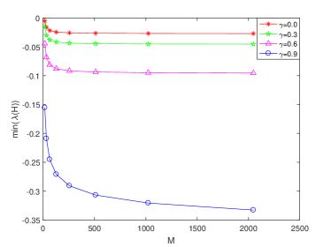
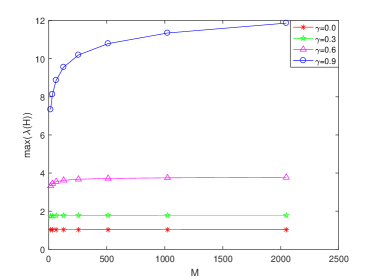
Fig. 1: The minimum and maximum eigenvalues of $H=\frac{\mathcal{A}+\mathcal{A}^{T}}{2}$.

3.2 Stability and convergence analysis for Crank-Nicolson scheme (5) in 1D

For steady-state nonlocal problem of (1), an optimal global convergence estimate with $\mathcal{O}\left(h^{3}\right)$ was established in [11]. However, for the time-dependent problems of (1), we next prove the stability and convergence with the superconvergence results.

Theorem 6.

The numerical schemes (5) is unconditionally stable.

Proof.

Let $\widetilde{u}_{i/2}^{k}~{}(i=1,2,\ldots,2M-1;\,k=0,1,\ldots,N)$ be the approximate solution of $u_{i/2}^{k}$, which is the exact solution of the difference scheme (5). Putting $\epsilon_{i/2}^{k}=\widetilde{u}_{i/2}^{k}-u_{i/2}^{k}$, then using (5), we obtain the following perturbation equation

$$\left(I+\frac{\tau}{2}\mathcal{A}\right)\varepsilon^{k}=\left(I-\frac{\tau}{2}\mathcal{A}\right)\varepsilon^{k-1},$$

with $\varepsilon^{k}=\left(\epsilon^{k}_{1},\epsilon^{k}_{2},\cdots,\epsilon^{k}_{M-1},\epsilon^{k}_{\frac{1}{2}},\epsilon^{k}_{\frac{3}{2}},\cdots,\epsilon^{k}_{M-\frac{1}{2}}\right)^{T}$. Upon relabeling and reorienting the vectors $\varepsilon^{k}$ as

$$\begin{split}\widetilde{\varepsilon}^{k}&=\left(\epsilon^{k}_{\frac{1}{2}},\epsilon^{k}_{1},\epsilon^{k}_{\frac{3}{2}},\epsilon^{k}_{2},\cdots,\epsilon^{k}_{M-1},\epsilon^{k}_{M-\frac{1}{2}}\right)^{T},\end{split}$$

then the above equation can be recast as

$$\left(I+\frac{\tau}{2}\widetilde{\mathcal{A}}\right)\widetilde{\varepsilon}^{k}=\left(I-\frac{\tau}{2}\widetilde{\mathcal{A}}\right)\widetilde{\varepsilon}^{k-1},$$

i.e.,

$$\left(1+\frac{\tau}{2}a_{i,i}\right)\epsilon^{k}_{\frac{i}{2}}=\epsilon^{k-1}_{\frac{i}{2}}-\frac{\tau}{2}\mathop{\sum}\limits_{j=1}^{2M-1}a_{i,j}\epsilon^{k-1}_{\frac{j}{2}}-\frac{\tau}{2}\sum^{2M-1}\limits_{j=1,j\neq i}a_{i,j}\epsilon^{k}_{\frac{j}{2}}~{}~{}{\rm with}~{}~{}\mathcal{\widetilde{A}}=\left\{a_{i,j}\right\}_{i,j=1}^{2M-1}.$$

Let $\left|\epsilon^{k}_{\frac{i_{0}}{2}}\right|:=\left|\left|\varepsilon^{k}\right|\right|_{\infty}=\mathop{\max}\limits_{1\leq i\leq 2M-1}|\epsilon^{k}_{\frac{i}{2}}|$. From Lemmas 3 and 4, it yields $a_{i,j}<0$, $i\neq j$, and $\sum^{2M-1}\limits_{j=1,j\neq i}\left|a_{i,j}\right|<a_{i,i}$, $0<a_{i,i}<C_{a}:=\frac{2\left(b-a\right)^{1-\gamma}}{1-\gamma}$,then

$$\begin{split}\left(1+\frac{\tau}{2}a_{i_{0},i_{0}}\right)\left|\left|\varepsilon^{k}\right|\right|_{\infty}&\leq\left|\epsilon^{k-1}_{\frac{i_{0}}{2}}\right|+\frac{\tau}{2}\mathop{\sum}\limits_{j=1}^{2M-1}\left|a_{i_{0},j}\right|\left|\epsilon^{k-1}_{\frac{j}{2}}\right|+\frac{\tau}{2}\mathop{\sum}^{2M-1}\limits_{j=1,j\neq i_{0}}\left|a_{i_{0},j}\right|\left|\epsilon^{k}_{\frac{j}{2}}\right|\\ &\leq\left|\left|\varepsilon^{k-1}\right|\right|_{\infty}+\frac{\tau}{2}\mathop{\sum}\limits_{j=1}^{2M-1}\left|a_{i_{0},j}\right|\left|\left|\varepsilon^{k-1}\right|\right|_{\infty}+\frac{\tau}{2}\mathop{\sum}^{2M-1}\limits_{j=1,j\neq i_{0}}\left|a_{i_{0},j}\right|\left|\left|\varepsilon^{k}\right|\right|_{\infty},\end{split}$$

it implies that

$$\left|\left|\varepsilon^{k}\right|\right|_{\infty}\leq\left(1+C_{a}\tau\right)\left|\left|\varepsilon^{k-1}\right|\right|_{\infty}\leq\left(1+C_{a}\tau\right)^{k}\left|\left|\varepsilon^{0}\right|\right|_{\infty}\leq\exp(TC_{a})\left|\left|\varepsilon^{0}\right|\right|_{\infty}.$$

The proof is completed. ∎

Theorem 7.

Let $u\left(x_{i/2},t_{k}\right)$ be the exact solution of (1) with $0<\gamma<1$, and $u_{i/2}^{k}$ the solution of the numerical scheme (5). Then

$$\begin{split}\left|\left|u(x_{i/2},t_{k})-u_{i/2}^{k}\right|\right|=\mathcal{O}\left(\tau^{2}+h^{4-\gamma}\right),\quad i=1,2,\ldots,2M-1;\,k=0,1,\ldots,N\end{split}$$

with $N\tau\leq T.$

Proof.

Denote $e_{i/2}^{k}=u(x_{i/2},t_{k})-u_{i/2}^{k}$, $i=1,2,\ldots,2M-1;\,k=0,1,\ldots,N$. Subtracting (5) from (1) with $E^{0}=0$, it yields

$$\left(I\!+\!\frac{\tau}{2}\mathcal{A}\right)E^{k}=\left(I\!-\!\frac{\tau}{2}\mathcal{A}\right)E^{k-1}\!+\!\tau R^{k-\frac{1}{2}},$$

with $E^{k}=\left(e^{k}_{1},e^{k}_{2},\cdots,e^{k}_{M-1},e^{k}_{\frac{1}{2}},e^{k}_{\frac{3}{2}},\cdots,e^{k}_{M-\frac{1}{2}}\right)^{T}$ and similarly for $R^{k-\frac{1}{2}}$. The local truncation error is $R_{i}^{k-\frac{1}{2}}=\mathcal{O}\left(\tau^{2}+h^{4}\left(\eta_{\frac{i}{2}}\right)^{-\gamma}\right)\leq C_{R}\left(\tau^{2}+h^{4-\gamma}\right)$, $\eta_{\frac{i}{2}}=\min\left\{x_{\frac{i}{2}}-a,b-x_{\frac{i}{2}}\right\}$ in (5) and $C_{R}$ is a constant.

Upon relabeling and reorienting the vectors $E^{k}$ and $R^{k-\frac{1}{2}}$ as

$$\widetilde{E}^{k}\!=\!\left(e^{k}_{\frac{1}{2}},e^{k}_{1},e^{k}_{\frac{3}{2}},e^{k}_{2},\cdots,e^{k}_{M-1},e^{k}_{M-\frac{1}{2}}\right)^{T}\!,$$

$$\widetilde{R}^{k\!-\!\frac{1}{2}}\!=\!\left(R^{k-\frac{1}{2}}_{\frac{1}{2}},R^{k-\frac{1}{2}}_{1},R^{k-\frac{1}{2}}_{\frac{3}{2}},R^{k-\frac{1}{2}}_{2},\cdots,R^{k-\frac{1}{2}}_{M-1},R_{M-\frac{1}{2}}\right)^{T},$$

then the above equation can be recast as

$$\left(I+\frac{\tau}{2}\widetilde{\mathcal{A}}\right)\widetilde{E}^{k}=\left(I-\frac{\tau}{2}\widetilde{\mathcal{A}}\right)\widetilde{E}^{k-1}+\tau\widetilde{R}^{k-\frac{1}{2}},$$

i.e.,

$$\left(1+\frac{\tau}{2}a_{i,i}\right)e^{k}_{\frac{i}{2}}=e^{k-1}_{\frac{i}{2}}-\frac{\tau}{2}\mathop{\sum}\limits_{j=1}^{2M-1}a_{i,j}e^{k-1}_{\frac{j}{2}}-\frac{\tau}{2}\sum^{2M-1}\limits_{j=1,j\neq i}a_{i,j}e^{k}_{\frac{j}{2}}+\tau R_{\frac{i}{2}}^{k-\frac{1}{2}}~{}~{}{\rm with}~{}~{}\mathcal{\widetilde{A}}=\left\{a_{i,j}\right\}_{i,j=1}^{2M-1}.$$

Let $\left|e^{k}_{\frac{i_{0}}{2}}\right|:=\left|\left|E^{k}\right|\right|_{\infty}=\mathop{\max}\limits_{1\leq i\leq 2M-1}\left|e^{k}_{\frac{i}{2}}\right|$. Using Lemmas 3 and 4, we get $a_{i,j}<0$, $i\neq j$, and $\sum^{2M-1}\limits_{j=1,j\neq i}\left|a_{i,j}\right|<a_{i,i}$, $0<a_{i,i}<C_{a}:=\frac{2\left(b-a\right)^{1-\gamma}}{1-\gamma}$. Therefore, we have

$$\begin{split}\left(1\!+\!\frac{\tau}{2}a_{i_{0},i_{0}}\right)\left|\left|E^{k}\right|\right|_{\infty}&\!\leq\!\left|e^{k-1}_{\frac{i_{0}}{2}}\right|+\frac{\tau}{2}\mathop{\sum}\limits_{j=1}^{2M-1}\left|a_{i_{0},j}\right|\left|e^{k-1}_{\frac{j}{2}}\right|+\frac{\tau}{2}\mathop{\sum}^{2M-1}\limits_{j=1,j\neq i_{0}}\left|a_{i_{0},j}\right|\left|e^{k}_{\frac{j}{2}}\right|+\tau\left|R_{\frac{i_{0}}{2}}^{k-\frac{1}{2}}\right|\\ &\!\leq\!\left(\!\!1\!+\!\frac{\tau}{2}\mathop{\sum}\limits_{j=1}^{2M-1}\left|a_{i_{0},j}\right|\right)\left|\left|E^{k-1}\right|\right|_{\infty}\!\!+\!\frac{\tau}{2}\mathop{\sum}^{2M-1}\limits_{j=1,j\neq i_{0}}\left|a_{i_{0},j}\right|\left|\left|E^{k}\right|\right|_{\infty}\!\!+\!\tau\left|R_{\frac{i_{0}}{2}}^{k-\frac{1}{2}}\right|.\end{split}$$

It leads to

$$\begin{split}\left|\left|E^{k}\right|\right|_{\infty}&\leq\left(1+\tau C_{a}\right)\left|\left|E^{k-1}\right|\right|_{\infty}+C_{R}\left(\tau^{2}+h^{4-\gamma}\right)\tau\\ &\leq\left(1+\tau C_{a}\right)^{k}\left|\left|E^{0}\right|\right|_{\infty}+C_{R}\left(\tau^{2}+h^{4-\gamma}\right)\tau\mathop{\sum}\limits^{k-1}_{l=0}\left(1+\tau C_{a}\right)^{l}\\ &\leq C_{R}\left(\tau^{2}+h^{4-\gamma}\right)\tau\mathop{\sum}\limits^{k-1}_{l=0}\left(1+\tau C_{a}\right)^{k}\leq C_{R}T\exp\left(TC_{a}\right)\left(\tau^{2}+h^{4-\gamma}\right).\end{split}$$

The proof is completed. ∎

3.3 Stability and convergence analysis for 2D with multiplicative Cauchy kernel

First, we provide a local truncation error analysis, which is still lacking in [11], for two-dimensional cases with multiplicative Cauchy kernel. Then the stability and convergence analysis are given.

Lemma 8.

Let ${\mathcal{A}}=\mathcal{D}_{x}\otimes\mathcal{D}_{y}-\mathcal{G}_{x}\otimes\mathcal{G}_{y}$ be given in (12). Then ${\mathcal{A}}$ is strictly diagonally dominant by rows.

Proof.

From Lemma 3, we known that $\mathcal{D}_{x}-\mathcal{G}_{x}$ and $\mathcal{D}_{y}-\mathcal{G}_{y}$ are strictly diagonally dominant by rows, and $\mathcal{G}_{x}$, $\mathcal{G}_{y}$ are positive matrices. Denote $\mathcal{D}_{x}=\{d^{x}_{i}\},\,\mathcal{G}_{x}=\{g^{x}_{i,l}\},\,i,l=1,2,\cdots,2M_{x}-1$, i.e.,

$$\begin{array}[]{cc}\mathcal{D}_{x}=\left(\begin{array}[]{cccc}d^{x}_{1}&{}\hfil&{}\hfil&{}\hfil\\ {}\hfil&d^{x}_{2}&{}\hfil&{}\hfil\\ {}\hfil&{}\hfil&\ddots&{}\hfil\\ {}\hfil&{}\hfil&{}\hfil&d^{x}_{2M_{x}-1}\end{array}\right)&\mathcal{G}_{x}=\left(\begin{array}[]{cccc}g^{x}_{1,1}&g^{x}_{1,2}&\cdots&g^{x}_{1,2M_{x}-1}\\[5.69054pt] g^{x}_{2,1}&g^{x}_{2,2}&\cdots&g^{x}_{2,2M_{x}-1}\\[5.69054pt] \vdots&\vdots&\ddots&\vdots\\[5.69054pt] g^{x}_{2M_{x}-1,1}&g^{x}_{2M_{x}-1,2}&\cdots&g^{x}_{2M_{x}-1,2M_{x}-1}\end{array}\right)\end{array}.$$

Similarly, we can denote $\mathcal{D}_{y}=\{d^{y}_{j}\},\,\mathcal{G}_{y}=\{g^{y}_{j,r}\},\,j,r=1,2,\cdots,2M_{y}-1$. Then

$$\begin{split}\mathcal{D}_{x}\otimes\mathcal{D}_{y}-\mathcal{G}_{x}\otimes\mathcal{G}_{y}=&\left(\begin{array}[]{cccc}d^{x}_{1}\otimes\mathcal{D}_{y}&{}\hfil&{}\hfil&{}\hfil\\ {}\hfil&d^{x}_{2}\otimes\mathcal{D}_{y}&{}\hfil&{}\hfil\\ {}\hfil&{}\hfil&\ddots&{}\hfil\\ {}\hfil&{}\hfil&{}\hfil&d^{x}_{2M_{x}-1}\otimes\mathcal{D}_{y}\end{array}\right)\\ &-\left(\begin{array}[]{cccc}g^{x}_{1,1}\otimes\mathcal{G}_{y}&g^{x}_{1,1}\otimes\mathcal{G}_{y}&\cdots&g^{x}_{1,2M_{x}-1}\otimes\mathcal{G}_{y}\\[5.69054pt] g^{x}_{2,1}\otimes\mathcal{G}_{y}&g^{x}_{2,2}\otimes\mathcal{G}_{y}&\cdots&g^{x}_{2,2M_{x}-1}\otimes\mathcal{G}_{y}\\[5.69054pt] \vdots&\vdots&\ddots&\vdots\\[5.69054pt] g^{x}_{2M_{x}-1,1}\otimes\mathcal{G}_{y}&g^{x}_{2M_{x}-1,2}\otimes\mathcal{G}_{y}&\cdots&g^{x}_{2M_{x}-1,2M_{x}-1}\otimes\mathcal{G}_{y}\end{array}\right),\end{split}$$

and the summation by rows in ${\mathcal{A}}$ can be expressed as $\left\{d^{x}_{i}d^{y}_{j}-\sum_{l=1}^{2M_{x}-1}g^{x}_{i,l}\sum_{r=1}^{2M_{y}-1}g^{y}_{j,r}\right\}$, since $d^{x}_{i}>\sum_{l=1}^{2M_{x}-1}g^{x}_{i,l}$ and $d^{y}_{j}>\sum_{r=1}^{2M_{x}-1}g^{y}_{j,r}$. The proof is completed. ∎

Lemma 9.

Let $0<\gamma<1$, $u(x,y)\in C^{6}\left(\left[a,b\right]\times\left[c,d\right]\right)$ and $u_{Q}(x,y)$ be defined by (9). Then for any $\left(x_{\frac{i}{2}},y_{\frac{j}{2}}\right)\in\left(a,b\right)\times\left(c,d\right)$, there exists

$$\int^{d}_{c}\int^{b}_{a}\frac{u\left(x,y\right)-u_{Q}\left(x,y\right)}{\left|x_{\frac{i}{2}}-x\right|^{\gamma}\left|y_{\frac{j}{2}}-y\right|^{\gamma}}dxdy=\mathcal{O}\left(h_{x}^{4}\left(\eta_{\frac{i}{2}}\right)^{-\gamma}+h_{y}^{4}\left(\widetilde{\eta}_{\frac{j}{2}}\right)^{-\gamma}\right)+\mathcal{O}\left(h_{x}^{5-\gamma}+h_{y}^{5-\gamma}\right),$$

with $\eta_{\frac{i}{2}}=\min\left\{x_{\frac{i}{2}}-a,b-x_{\frac{i}{2}}\right\},\ \widetilde{\eta}_{\frac{j}{2}}=\min\left\{y_{\frac{j}{2}}-c,d-y_{\frac{j}{2}}\right\},\ i=1,2\ldots,2M_{x}-1,\ j=1,2\ldots,2M_{y}-1.$

Proof.

Let $\left(x,y\right)\in\left[x_{\frac{l}{2}},x_{\frac{l}{2}+1}\right]\times\left[y_{\frac{r}{2}},y_{\frac{r}{2}+1}\right]$, $l=0,1,2\ldots,2M_{x}-2$, $r=0,1,2\ldots,2M_{y}-2$. Using Taylor expansion and (9), there exist $\xi_{\frac{l}{2}}\in\left[x_{\frac{l}{2}},x_{\frac{l}{2}+1}\right]$, $\zeta_{\frac{r}{2}}\in\left[y_{\frac{r}{2}},y_{\frac{r}{2}+1}\right]$ and $\varsigma_{\frac{r}{2}}\in\left[y_{\frac{r}{2}},y_{\frac{r}{2}+1}\right]$ such that

$$\begin{split}u\left(x,y\right)-u_{Q}\left(x,y\right)&=u\left(x,y\right)-\sum^{2}_{s=0}\phi_{\frac{l+s}{2}}(x)u\left(x_{\frac{l+s}{2}},y\right)\\ &\qquad+\sum^{2}_{s=0}\phi_{\frac{l+s}{2}}(x)u\left(x_{\frac{l+s}{2}},y\right)-\sum^{2}_{t=0}\phi_{\frac{r+t}{2}}(y)\sum^{2}_{s=0}\phi_{\frac{l+s}{2}}(x)u\left(x_{\frac{l+s}{2}},y_{\frac{r+t}{2}}\right)\\ &=:E_{x}+E_{y}+E_{xy},\end{split}$$

where

$$\begin{split}E_{x}&=\frac{u^{(3)}_{x}\left(\xi_{\frac{l}{2}},y\right)}{3!}\left(x-x_{\frac{l}{2}}\right)\left(x-x_{\frac{l+1}{2}}\right)\left(x-x_{\frac{l}{2}+1}\right),\\ E_{y}&=\frac{u^{(3)}_{y}\left(x,\zeta_{\frac{r}{2}}\right)}{3!}\left(y-y_{\frac{r}{2}}\right)\left(y-y_{\frac{r+1}{2}}\right)\left(y-y_{\frac{r}{2}+1}\right),\end{split}$$

and

$$\begin{split}E_{xy}=\frac{-1}{(3!)^{2}}\frac{\partial^{6}u\left(\varsigma_{\frac{r}{2}},\zeta_{\frac{r}{2}}\right)}{\partial x^{3}\partial y^{3}}\left(x\!-x_{\frac{l}{2}}\right)\!\left(x\!-x_{\frac{l+1}{2}}\right)\!\left(x\!-x_{\frac{l}{2}+1}\right)\!\left(y\!-y_{\frac{r}{2}}\right)\!\left(y\!-y_{\frac{r+1}{2}}\right)\!\left(y\!-y_{\frac{r}{2}+1}\right).\end{split}$$

Form Theorem $3.7$ of [11] and Lemma 4, for any $\left(x_{\frac{i}{2}},y_{\frac{j}{2}}\right)\in\left(a,b\right)\times\left(c,d\right)$, $i=1,2\ldots,2M_{x}-1$, $j=1,2\ldots,2M_{y}-1$, we have

$$\begin{split}&\left|\!\int^{d}_{c}\!\int^{b}_{a}\frac{u\left(x,y\right)-u_{Q}\left(x,y\right)}{\left|x_{\frac{i}{2}}-x\right|^{\gamma}\left|y_{\frac{j}{2}}-y\right|^{\gamma}}dxdy\right|=\left|\sum^{2M_{y}-2}_{r=0}\!\sum^{2M_{x}-2}_{l=0}\!\int^{y_{\frac{r}{2}+1}}_{y_{\frac{r}{2}}}\!\int^{x_{\frac{l}{2}+1}}_{x_{\frac{l}{2}}}\!\frac{E_{x}+E_{y}+E_{xy}}{\left|x_{\frac{i}{2}}-x\right|^{\gamma}\left|y_{\frac{j}{2}}-y\right|^{\gamma}}dxdy\right|\\ \leq&\left|\sum^{2M_{x}-2}_{l=0}\!\int^{x_{\frac{l}{2}+1}}_{x_{\frac{l}{2}}}\frac{E_{x}}{\left|x_{\frac{i}{2}}-x\right|^{\gamma}}dx\!\int^{d}_{c}\!\frac{1}{\left|y_{\frac{j}{2}}-y\right|^{\gamma}}dy\right|\!+\!\left|\!\int^{b}_{a}\frac{1}{\left|x_{\frac{i}{2}}-x\right|^{\gamma}}dx\!\sum^{2M_{y}-2}_{r=0}\!\int^{y_{\frac{r}{2}+1}}_{y_{\frac{r}{2}}}\frac{E_{y}+E_{xy}}{\left|y_{\frac{j}{2}}-y\right|^{\gamma}}dy\right|\\ =&\mathcal{O}\left(h_{x}^{4}\left(\eta_{\frac{i}{2}}\right)^{-\gamma}\right)+\mathcal{O}\left(h_{x}^{5-\gamma}\right)+\mathcal{O}\left(h_{y}^{4}\left(\widetilde{\eta}_{\frac{j}{2}}\right)^{-\gamma}\right)+\mathcal{O}\left(h_{y}^{5-\gamma}\right)+\mathcal{O}\left(h_{x}^{3}h_{y}^{3}\right)\end{split}$$

with $\eta_{\frac{i}{2}}=\min\left\{x_{\frac{i}{2}}-a,b-x_{\frac{i}{2}}\right\},\ \widetilde{\eta}_{\frac{j}{2}}=\min\left\{y_{\frac{j}{2}}-c,d-y_{\frac{j}{2}}\right\}$. The proof is completed. ∎

Theorem 10.

The numerical schemes (14) is unconditionally stable.

Proof.

Let $\widetilde{u}_{\frac{i}{2},\frac{j}{2}}^{k}~{}(i=1,2,\ldots,2M_{x}-1;j=1,2,\ldots,2M_{y}-1;\,k=0,1,\ldots,N)$ be the approximate solution of $u_{\frac{i}{2},\frac{j}{2}}^{k}$, which is the exact solution of the difference scheme (14). Putting $\epsilon_{\frac{i}{2},\frac{j}{2}}^{k}=\widetilde{u}_{\frac{i}{2},\frac{j}{2}}^{k}-u_{\frac{i}{2},\frac{j}{2}}^{k}$, and we denote

$$\varepsilon_{i}^{k}=\left(\epsilon_{i,1}^{k},\epsilon_{i,2}^{k},\cdots,\epsilon_{i,M_{y}-1}^{k},\epsilon_{i,\frac{1}{2}}^{k},\epsilon_{i,\frac{3}{2}}^{k},\cdots,\epsilon_{i,M_{y}-\frac{1}{2}}^{k}\right),\ i=1,2,\cdots,M_{x}-1,\textstyle\frac{1}{2},\frac{3}{2},\cdots,M_{x}-\frac{1}{2}$$

then using (14), we obtain the following perturbation equation

$$\left(I+\frac{\tau}{2}{\mathcal{A}}\right){\varepsilon}^{k}=\left(I-\frac{\tau}{2}{\mathcal{A}}\right){\varepsilon}^{k-1},$$

with ${\varepsilon}^{k}=\left(\varepsilon_{1}^{k},\varepsilon_{2}^{k},\cdots,\varepsilon_{M_{x}-1}^{k},\varepsilon_{\frac{1}{2}}^{k},\varepsilon_{\frac{3}{2}}^{k},\cdots,\varepsilon_{M_{x}-\frac{1}{2}}^{k}\right)^{T}$. Upon relabeling and reorienting the vectors ${\varepsilon}^{k}$ as

$$\widetilde{{\varepsilon}}^{k}=\left(\widetilde{\varepsilon}^{k}_{\frac{1}{2}},\widetilde{\varepsilon}^{k}_{1},\widetilde{\varepsilon}^{k}_{\frac{3}{2}},\widetilde{\varepsilon}^{k}_{2},\cdots,\widetilde{\varepsilon}^{k}_{M_{x}-1},\widetilde{\varepsilon}^{k}_{M_{x}-\frac{1}{2}}\right)^{T},$$

where

$$\widetilde{\varepsilon}_{i}^{k}=\left(\epsilon_{i,\frac{1}{2}}^{k},\epsilon_{i,1}^{k},\epsilon_{i,\frac{3}{2}}^{k},\epsilon_{i,2}^{k},\cdots,\epsilon_{i,M_{y}-1}^{k},\epsilon_{i,M_{y}-\frac{1}{2}}^{k}\right),\ i=1,\frac{1}{2},2,\frac{3}{2},\cdots,M_{x}-1,M_{x}-\frac{1}{2},$$

then the above equation can be recast as

$$\left(I+\frac{\tau}{2}\widetilde{{\mathcal{A}}}\right)\widetilde{{\varepsilon}}^{k}=\left(I-\frac{\tau}{2}\widetilde{{\mathcal{A}}}\right)\widetilde{{\varepsilon}}^{k-1}~{}~{}{\rm with}~{}~{}\widetilde{{\mathcal{A}}}=\widetilde{\mathcal{D}}_{x}\otimes\widetilde{\mathcal{D}}_{y}-\widetilde{\mathcal{G}}_{x}\otimes\widetilde{\mathcal{G}}_{y},$$

where $\widetilde{\mathcal{D}}_{x}=\left\{d^{x}_{i}\right\},\ \widetilde{\mathcal{G}}_{x}=\left\{g^{x}_{i,l}\right\},\,\textstyle i,l=1,2,\ldots,{2M_{x}-1}$, $\widetilde{\mathcal{D}}_{y}=\left\{d^{y}_{j}\right\},\ \widetilde{\mathcal{G}}_{y}=\left\{g^{y}_{j,r}\right\},\,\textstyle j,r=1,2,\ldots,{2M_{y}-1}$, i.e.,

$$\left(1\!+\frac{\tau}{2}d^{x}_{i}d^{y}_{j}\right)\epsilon_{\frac{i}{2},\frac{j}{2}}^{k}-\frac{\tau}{2}\mathop{\sum}\limits_{l=1}^{2M_{x}-1}\!\mathop{\sum}\limits_{r=1}^{2M_{y}-1}\!g^{x}_{i,l}g^{y}_{j,r}\epsilon_{\frac{l}{2},\frac{r}{2}}^{k}\!=\!\left(1\!-\frac{\tau}{2}d^{x}_{i}d^{y}_{j}\right)\epsilon_{\frac{i}{2},\frac{j}{2}}^{k-1}+\frac{\tau}{2}\mathop{\sum}\limits_{l=1}^{2M_{x}-1}\!\mathop{\sum}\limits_{r=1}^{2M_{y}-1}\!g^{x}_{i,l}g^{y}_{j,r}\epsilon_{\frac{l}{2},\frac{r}{2}}^{k-1}.$$

Let $\left|\epsilon^{k}_{\frac{i_{0}}{2},\frac{j_{0}}{2}}\right|:=\left|\left|{\varepsilon}^{k}\right|\right|_{\infty}=\mathop{\max}\limits_{i,j}\left|\epsilon^{k}_{\frac{i}{2},\frac{j}{2}}\right|$. From Lemmas 3 and 4, it yields $0\!<d^{x}_{i}d^{y}_{j}\!<C_{d}\!:=\frac{4\left(b-a\right)^{1-\gamma}\left(d-c\right)^{1-\gamma}}{\left(1-\gamma\right)^{2}}$, using Theorem 6 and Lemma 8, we have

$$\begin{split}&\left(1+\frac{\tau}{2}d^{x}_{i_{0}}d^{y}_{j_{0}}\right)\left|\left|{\varepsilon}^{k}\right|\right|_{\infty}\\ \leq&\left|\epsilon_{\frac{i_{0}}{2},\frac{j_{0}}{2}}^{k-1}\right|\!+\!\frac{\tau}{2}d^{x}_{i_{0}}d^{y}_{j_{0}}\left|\epsilon_{\frac{i_{0}}{2},\frac{j_{0}}{2}}^{k-1}\right|\!+\!\frac{\tau}{2}\mathop{\sum}\limits_{l=1}^{2M_{x}-1}\mathop{\sum}\limits_{r=1}^{2M_{y}-1}g^{x}_{i_{0},l}g^{y}_{j_{0},r}\left|\epsilon_{\frac{l}{2},\frac{r}{2}}^{k-1}\right|\!+\!\frac{\tau}{2}\mathop{\sum}\limits_{l=1}^{2M_{x}-1}\mathop{\sum}\limits_{r=1}^{2M_{y}-1}g^{x}_{i_{0},l}g^{y}_{j_{0},r}\left|\epsilon_{\frac{l}{2},\frac{r}{2}}^{k}\right|\\ \!\leq&\left|\left|{\varepsilon}^{k-1}\right|\right|_{\infty}\!+\!\frac{\tau}{2}\left(\!\!d^{x}_{i_{0}}d^{y}_{j_{0}}\!+\!\mathop{\sum}\limits_{l=1}^{2M_{x}-1}\mathop{\sum}\limits_{r=1}^{2M_{y}-1}g^{x}_{i_{0},l}g^{y}_{j_{0},r}\!\!\right)\left|\left|{\varepsilon}^{k-1}\right|\right|_{\infty}\!+\!\frac{\tau}{2}\sum\limits_{l=1}^{2M_{x}-1}\sum\limits_{r=1}^{2M_{y}-1}g^{x}_{i_{0},l}g^{y}_{j_{0},r}\left|\left|{\varepsilon}^{k}\right|\right|_{\infty},\end{split}$$

which leads to

$$\left|\left|{\varepsilon}^{k}\right|\right|_{\infty}\leq\left(1+\tau C_{d}\right)\left|\left|{\varepsilon}^{k-1}\right|\right|_{\infty}\leq\left(1+\tau C_{d}\right)^{k}\left|\left|{\varepsilon}^{0}\right|\right|_{\infty}\leq\exp\left(TC_{d}\right)\left|\left|{\varepsilon}^{0}\right|\right|_{\infty}.$$

The proof is completed. ∎

Theorem 11.

Let $u\left(x_{\frac{i}{2}},y_{\frac{j}{2}},t_{k}\right)$ be the exact solution of (13) with $0<\gamma<1$, and $u_{\frac{i}{2},\frac{j}{2}}^{k}$ the solution of the numerical scheme (14). Then

$$\begin{split}\left|\left|u\left(x_{\frac{i}{2}},y_{\frac{j}{2}},t_{k}\right)-u_{\frac{i}{2},\frac{j}{2}}^{k}\right|\right|=\mathcal{O}\left(\tau^{2}+h_{x}^{4-\gamma}+h_{y}^{4-\gamma}\right),\end{split}$$

with $i=1,2,\ldots,2M_{x}-1;j=1,2,\ldots,2M_{y}-1;\,k=0,1,\ldots,N$ and $N\tau\leq T$.

Proof.

Denote $e_{\frac{i}{2},\frac{j}{2}}^{k}=u\left(x_{\frac{i}{2}},y_{\frac{j}{2}},t_{k}\right)-u_{\frac{i}{2},\frac{j}{2}}^{k}$, and

$$E_{i}^{k}=\left(e_{i,1}^{k},e_{i,2}^{k},\cdots,e_{i,M_{y}-1}^{k},e_{i,\frac{1}{2}}^{k},e_{i,\frac{3}{2}}^{k},\cdots,e_{i,M_{y}-\frac{1}{2}}^{k}\right),\ i=1,2,\cdots,M_{x}-1,\textstyle\frac{1}{2},\frac{3}{2},\cdots,M_{x}-\frac{1}{2}$$

Subtracting (14) from (13) with ${E}^{0}={0}$, a zero vector, it yields

$$\left(I+\frac{\tau}{2}{\mathcal{A}}\right){E}^{k}=\left(I-\frac{\tau}{2}{\mathcal{A}}\right){E}^{k-1}+\tau{R}^{k-\frac{1}{2}},$$

with ${E}^{k}=\left(E^{k}_{1},E^{k}_{2},\cdots,E^{k}_{M_{x}-1},E^{k}_{\frac{1}{2}},E^{k}_{\frac{3}{2}},\cdots,E^{k}_{M_{x}-\frac{1}{2}}\right)^{T}$ and similarly for ${R}^{k-\frac{1}{2}}$. Here the local truncation error is ${R}_{\frac{i}{2},\frac{j}{2}}^{k-\frac{1}{2}}=\mathcal{O}\!\left(\!\tau^{2}+h^{4}\left(\eta_{\frac{i}{2}}\right)^{-\gamma}\!+\!h^{4}\left(\widetilde{\eta}_{\frac{j}{2}}\right)^{-\gamma}\!\right)\leq C_{R}\left(\tau^{2}\!+\!h_{x}^{4-\gamma}+h_{y}^{4-\gamma}\right)$, with $\eta_{\frac{i}{2}}=\min\left\{x_{\frac{i}{2}}-a,b-x_{\frac{i}{2}}\right\},\widetilde{\eta}_{\frac{j}{2}}=\min\left\{y_{\frac{j}{2}}-c,d-y_{\frac{j}{2}}\right\}$ in (14) and $C_{R}$ is a constant.

Upon relabeling and reorienting the vectors ${E}^{k}$ and ${R}^{k-\frac{1}{2}}$ as $\widetilde{{E}}^{k}$ and $\widetilde{{R}}^{k-\frac{1}{2}}$ as in Theorem 10 again, then the above equation can be recast as

$$\left(I+\frac{\tau}{2}\widetilde{{\mathcal{A}}}\right)\widetilde{{E}}^{k}=\left(I-\frac{\tau}{2}\widetilde{{\mathcal{A}}}\right)\widetilde{{E}}^{k-1}+\tau\widetilde{{R}}^{k-\frac{1}{2}},~{}~{}{\rm with}~{}~{}\widetilde{{\mathcal{A}}}=\widetilde{\mathcal{D}}_{x}\otimes\widetilde{\mathcal{D}}_{y}-\widetilde{\mathcal{G}}_{x}\otimes\widetilde{\mathcal{G}}_{y},$$

where $\widetilde{\mathcal{D}}_{x}=\left\{d^{x}_{i}\right\},\ \widetilde{\mathcal{G}}_{x}=\left\{g^{x}_{i,l}\right\},\ \textstyle i,l=1,2,\ldots,{2M_{x}-1}$, $\widetilde{\mathcal{D}}_{y}=\left\{d^{y}_{j}\right\},\ \widetilde{\mathcal{G}}_{y}=\left\{g^{y}_{j,r}\right\},\ \textstyle j,r=1,2,\ldots,{2M_{y}-1}$, i.e.,

$$\begin{split}&\left(1+\frac{\tau}{2}d^{x}_{i}d^{y}_{j}\right)e_{\frac{i}{2},\frac{j}{2}}^{k}-\frac{\tau}{2}\mathop{\sum}\limits_{l=1}^{2M_{x}-1}\mathop{\sum}\limits_{r=1}^{2M_{y}-1}g^{x}_{i,l}g^{y}_{j,r}e_{\frac{l}{2},\frac{r}{2}}^{k}\\ &\quad=\left(1-\frac{\tau}{2}d^{x}_{i}d^{y}_{j}\right)e_{\frac{i}{2},\frac{j}{2}}^{k-1}+\frac{\tau}{2}\mathop{\sum}\limits_{l=1}^{2M_{x}-1}\mathop{\sum}\limits_{r=1}^{2M_{y}-1}g^{x}_{i,l}g^{y}_{j,r}e_{\frac{l}{2},\frac{r}{2}}^{k-1}+\tau R_{\frac{i}{2},\frac{j}{2}}^{k-\frac{1}{2}}.\end{split}$$

Let $\left|e^{k}_{\frac{i_{0}}{2},\frac{j_{0}}{2}}\right|:=\left|\left|{E}^{k}\right|\right|_{\infty}=\mathop{\max}\limits_{i,j}\left|e^{k}_{\frac{i}{2},\frac{j}{2}}\right|$. Using Lemmas 3 and 4, we get $0<d_{i}d_{j}<C_{d}:=\frac{4\left(b-a\right)^{1-\gamma}\left(d-c\right)^{1-\gamma}}{(1-\gamma)^{2}}$, combine with Theorem 7 and Lemma 8, we have

$$\begin{split}\left(1\!+\!\frac{\tau}{2}d^{x}_{i_{0}}d^{y}_{j_{0}}\right)\left|\left|{E}^{k}\right|\right|_{\infty}\leq&\left|e_{\frac{i_{0}}{2},\frac{j_{0}}{2}}^{k-1}\right|\!+\!\frac{\tau}{2}d^{x}_{i_{0}}d^{y}_{j_{0}}\left|e_{\frac{i_{0}}{2},\frac{j_{0}}{2}}^{k-1}\right|\!+\!\frac{\tau}{2}\mathop{\sum}\limits_{l=1}^{2M_{x}-1}\mathop{\sum}\limits_{r=1}^{2M_{y}-1}g^{x}_{i_{0},l}g^{y}_{j_{0},r}\left|e_{\frac{l}{2},\frac{r}{2}}^{k-1}\right|\\ &\!+\!\frac{\tau}{2}\mathop{\sum}\limits_{l=1}^{2M_{x}-1}\mathop{\sum}\limits_{r=1}^{2M_{y}-1}g^{x}_{i_{0},l}g^{y}_{j_{0},r}\left|e_{\frac{l}{2},\frac{r}{2}}^{k}\right|\!+\!\tau\left|R_{\frac{i_{0}}{2},\frac{j_{0}}{2}}^{k-\frac{1}{2}}\right|\\ \!\leq\!&\left(1\!+\!\tau C_{d}\right)\left|\left|{E}^{k-1}\right|\right|_{\infty}\!\!+\!\frac{\tau}{2}\mathop{\sum}\limits_{l=1}^{2M_{x}-1}\mathop{\sum}\limits_{r=1}^{2M_{y}-1}\!\!g^{x}_{i_{0},l}g^{y}_{j_{0},r}\left|\left|{E}^{k}\right|\right|_{\infty}\!\!\!+\!\tau\left|R_{\frac{i_{0}}{2},\frac{j_{0}}{2}}^{k-\frac{1}{2}}\right|,\end{split}$$

which leads to

$$\begin{split}\left|\left|{E}^{k}\right|\right|_{\infty}&\leq\left(1+\tau C_{d}\right)\left|\left|{E}^{k-1}\right|\right|_{\infty}+C_{R}\left(\tau^{2}+h_{x}^{4-\gamma}+h_{y}^{4-\gamma}\right)\tau\\ &\leq\left(1+\tau C_{d}\right)^{k}\left|\left|{E}^{0}\right|\right|_{\infty}+C_{R}\left(\tau^{2}+h_{x}^{4-\gamma}+h_{y}^{4-\gamma}\right)\tau\mathop{\sum}\limits^{k-1}_{l=0}\left(1+\tau C_{d}\right)^{l}\\ &\leq C_{R}\left(\tau^{2}+h_{x}^{4-\gamma}+h_{y}^{4-\gamma}\right)\tau\mathop{\sum}\limits^{k-1}_{l=0}\left(1+\tau C_{d}\right)^{k}\leq C_{R}T\exp\left(TC_{d}\right)\left(\tau^{2}+h_{x}^{4-\gamma}+h_{y}^{4-\gamma}\right).\end{split}$$

The proof is completed. ∎

3.4 Stability and convergence analysis for 2D with additive Cauchy kernels

It should be noted that the stiffness matrix (12) with multiplicative Cauchy kernels can be computed explicitly, but it is not for additive Cauchy kernels.

Lemma 12.

Let $0<\gamma<1$, $u(x,y)\in C^{6}\left(\left[a,b\right]\times\left[c,d\right]\right)$ and $u_{Q}(x,y)$ be defined by (9). Then for any $\left(x_{\frac{i}{2}},y_{\frac{j}{2}}\right)\in\left(a,b\right)\times\left(c,d\right)$, there exists

$$\int^{d}_{c}\int^{b}_{a}\frac{u\left(x,y\right)-u_{Q}\left(x,y\right)}{\left|\sqrt{\left(x_{\frac{i}{2}}-x\right)^{2}\!\!+\!\!\left(y_{\frac{j}{2}}-y\right)^{2}}\right|^{\gamma}}dxdy=\mathcal{O}\left(h_{x}^{4}\left(\eta_{\frac{i}{2}}\right)^{-\gamma}\!+\!h_{y}^{4}\left(\widetilde{\eta}_{\frac{j}{2}}\right)^{-\gamma}\right)+\mathcal{O}\left(h_{x}^{5-\gamma}\!+\!h_{y}^{5-\gamma}\right),$$

with $\eta_{\frac{i}{2}}=\min\left\{x_{\frac{i}{2}}-a,b-x_{\frac{i}{2}}\right\},\ \widetilde{\eta}_{\frac{j}{2}}=\min\left\{y_{\frac{j}{2}}-c,d-y_{\frac{j}{2}}\right\}i=1,2\ldots,2M_{x}-1,\ j=1,2\ldots,2M_{y}-1.$

Proof.

According to (3.3), Lemma 4 and Theorem $3.7$ in [11], for any $\left(x_{\frac{i}{2}},y_{\frac{j}{2}}\right)\in\left(a,b\right)\times\left(c,d\right)$, $i=1,2\ldots,2M_{x}-1$, $j=1,2\ldots,2M_{y}-1$, we have

$$\begin{split}&\left|\int^{d}_{c}\int^{b}_{a}\frac{u\left(x,y\right)-u_{Q}\left(x,y\right)}{\left|\sqrt{\left(x_{i/2}-x\right)^{2}+\left(y_{j/2}-y\right)^{2}}\right|^{\gamma}}dxdy\right|\\ \!\leq&\left|\sum^{2M_{x}-2}_{l=0}\int^{x_{\frac{l}{2}+1}}_{x_{\frac{l}{2}}}\frac{E_{x}}{\left|x_{i/2}-x\right|^{\gamma}}dx\int^{d}_{c}\frac{1}{\left|\sqrt{1\!+\left(\frac{y_{j/2}-y}{x_{i/2}-x}\right)^{2}}\right|^{\gamma}}dy\right|\\ &\!+\left|\int^{b}_{a}\frac{1}{\left|\sqrt{\left(\frac{x_{i/2}-x}{y_{j/2}-y}\right)^{2}+1}\right|^{\gamma}}dx\sum^{2M_{y}-2}_{r=0}\int^{y_{\frac{r}{2}\!+1}}_{y_{\frac{r}{2}}}\frac{E_{y}+E_{xy}}{|y_{j/2}-y|^{\gamma}}dy\right|\\ =&\mathcal{O}\left(h_{x}^{4}\left(\eta_{\frac{i}{2}}\right)^{-\gamma}\right)\!+\mathcal{O}\left(h_{x}^{5-\gamma}\right)+\mathcal{O}\left(h_{y}^{4}\left(\widetilde{\eta}_{\frac{j}{2}}\right)^{-\gamma}\right)+\mathcal{O}\left(h_{y}^{5-\gamma}\right)+\mathcal{O}\left(h_{x}^{3}h_{y}^{3}\right)\end{split}$$

with $\eta_{\frac{i}{2}}=\min\left\{x_{\frac{i}{2}}-a,b-x_{\frac{i}{2}}\right\},\ \widetilde{\eta}_{\frac{j}{2}}=\min\left\{y_{\frac{j}{2}}-c,d-y_{\frac{j}{2}}\right\}$. The proof is completed. ∎

Theorem 13.

The numerical schemes (21) is unconditionally stable.

Proof.

Let $\widetilde{u}_{\frac{i}{2},\frac{j}{2}}^{k}~{}(i=1,2\ldots,2M_{x}-1;\,j=1,2\ldots,2M_{y}-1;\,k=0,1,\ldots,N)$ be the approximate solution of $u_{\frac{i}{2},\frac{j}{2}}^{k}$, which is the exact solution of the difference scheme (21). Putting $\epsilon_{\frac{i}{2},\frac{j}{2}}^{k}=\widetilde{u}_{\frac{i}{2},\frac{j}{2}}^{k}-u_{\frac{i}{2},\frac{j}{2}}^{k}$, and we denote

$$\varepsilon_{i}^{k}=\left(\epsilon_{i,1}^{k},\epsilon_{i,2}^{k},\cdots,\epsilon_{i,M_{y}-1}^{k},\epsilon_{i,\frac{1}{2}}^{k},\epsilon_{i,\frac{3}{2}}^{k},\cdots,\epsilon_{i,M_{y}-\frac{1}{2}}^{k}\right),\ i=1,2,\cdots,M_{x}-1,\textstyle\frac{1}{2},\frac{3}{2},\cdots,M_{x}-\frac{1}{2},$$

then using (21), we obtain the following perturbation equation

$$\left(I+\frac{\tau}{2}{\mathcal{A}}\right){\varepsilon}^{k}=\left(I-\frac{\tau}{2}{\mathcal{A}}\right){\varepsilon}^{k-1},$$

with ${\varepsilon}^{k}=\left(\varepsilon_{1}^{k},\varepsilon_{2}^{k},\cdots,\varepsilon_{M_{x}-1}^{k},\varepsilon_{\frac{1}{2}}^{k},\varepsilon_{\frac{3}{2}}^{k},\cdots,\varepsilon_{M_{x}-\frac{1}{2}}^{k}\right)^{T}$. Upon relabeling and reorienting the vectors ${\varepsilon}^{k}$ as

$$\widetilde{{\varepsilon}}^{k}=\left(\widetilde{\varepsilon}^{k}_{\frac{1}{2}},\widetilde{\varepsilon}^{k}_{1},\widetilde{\varepsilon}^{k}_{\frac{3}{2}},\widetilde{\varepsilon}^{k}_{2},\cdots,\widetilde{\varepsilon}^{k}_{M_{x}-1},\widetilde{\varepsilon}^{k}_{M_{x}-\frac{1}{2}}\right)^{T},$$

where

$$\widetilde{\varepsilon}_{i}^{k}=\left(\epsilon_{i,\frac{1}{2}}^{k},\epsilon_{i,1}^{k},\epsilon_{i,\frac{3}{2}}^{k},\epsilon_{i,2}^{k},\cdots,\epsilon_{i,M_{y}-1}^{k},\epsilon_{i,M_{y}-\frac{1}{2}}^{k}\right),\ i=\textstyle\frac{1}{2},1,\textstyle\frac{3}{2},2,\cdots,M_{x}-1,\textstyle M_{x}-\frac{1}{2},$$

then the above equation can be recast as

$$\left(I+\frac{\tau}{2}\widetilde{{\mathcal{A}}}\right)\widetilde{{\varepsilon}}^{k}=\left(I-\frac{\tau}{2}\widetilde{{\mathcal{A}}}\right)\widetilde{{\varepsilon}}^{k-1},~{}~{}{\rm with}~{}~{}\widetilde{{\mathcal{A}}}=\widetilde{{\mathcal{D}}}-\widetilde{{\mathcal{G}}},$$

where $\widetilde{{\mathcal{D}}}=\left\{{d}_{i,j}\right\},\widetilde{{\mathcal{G}}}=\left\{{g}_{i,j}^{l,r}\right\},\,i,l=1,2,\ldots,{2M_{x}-1};\,j,r=1,2,\ldots,{2M_{y}-1}$, i.e.,

$$\left(1+\frac{\tau}{2}{d}_{i,j}\right)\epsilon_{\frac{i}{2},\frac{j}{2}}^{k}-\frac{\tau}{2}\mathop{\sum}\limits_{l=1}^{2M_{x}-1}\mathop{\sum}\limits_{r=1}^{2M_{y}-1}{g}_{i,j}^{l,r}\epsilon_{\frac{l}{2},\frac{r}{2}}^{k}=\left(1-\frac{\tau}{2}{d}_{i,j}\right)\epsilon_{\frac{i}{2},\frac{j}{2}}^{k-1}+\frac{\tau}{2}\mathop{\sum}\limits_{l=1}^{2M_{x}-1}\mathop{\sum}\limits_{r=1}^{2M_{y}-1}{g}_{i,j}^{l.r}\epsilon_{\frac{l}{2},\frac{r}{2}}^{k-1}.$$

Let $\left|\epsilon^{k}_{\frac{i_{0}}{2},\frac{j_{0}}{2}}\right|:=\left|\left|{\varepsilon}^{k}\right|\right|_{\infty}=\mathop{\max}\limits_{i,j}\left|\epsilon^{k}_{\frac{i}{2},\frac{j}{2}}\right|$. Since

$$\begin{split}\int_{a}^{b}\int_{c}^{d}\!\frac{1}{\left|\sqrt{\left(x_{i/2}-\bar{x}\right)^{2}\!+\!\left(y_{j/2}-\bar{y}\right)^{2}}\right|^{\gamma}}d\bar{x}d\bar{y}&\!=\!\int^{b}_{a}\int^{d}_{c}\!\frac{1}{\left|\sqrt{\left(\frac{x_{i/2}-\bar{x}}{y_{j/2}-\bar{y}}\right)^{2}\!+\!1}\right|^{\gamma}}\frac{1}{|y_{j/2}\!-\!\bar{y}|^{\gamma}}d\bar{x}d\bar{y}\\ &\!\leq\!\int^{b}_{a}\int^{d}_{c}\!\frac{1}{|y_{j/2}-\bar{y}|^{\gamma}}d\bar{x}d\bar{y}\leq C_{d},\end{split}$$

with $0\!<{d}_{i,j}\leq C_{d}=\frac{2(b-a)(d-c)^{1-\gamma}}{(1-\gamma)}$. From (7) and (8), we have

$$\begin{split}&\mathop{\sum}\limits_{l=1}^{2M_{x}-1}\mathop{\sum}\limits_{r=1}^{2M_{y}-1}\left|{g}_{i_{0},j_{0}}^{l,r}\right|\\ \leq&\mathop{\sum}\limits_{l=0}^{2M_{x}-1}\mathop{\sum}\limits_{r=0}^{2M_{y}-1}\left|\int^{x_{l+1}}_{x_{l}}\int^{y_{r+1}}_{y_{r}}\frac{\left(|\phi^{+}_{l}|+|\phi_{l+\frac{1}{2}}|+|\phi^{-}_{l+1}|\right)\left(|\phi^{+}_{r}|+|\phi_{r+\frac{1}{2}}|+|\phi^{-}_{r+1}|\right)}{\left|\sqrt{\left(x_{i/2}-\bar{x}\right)^{2}+\left(y_{j/2}-\bar{y}\right)^{2}}\right|^{\gamma}}d\bar{x}d\bar{y}\right|\\ \leq&9\mathop{\sum}\limits_{l=0}^{2M_{x}-1}\mathop{\sum}\limits_{r=0}^{2M_{y}-1}\left|\int^{x_{l+1}}_{x_{l}}\int^{y_{r+1}}_{y_{r}}\frac{1}{\left|\sqrt{\left(x_{i/2}-\bar{x}\right)^{2}+\left(y_{j/2}-\bar{y}\right)^{2}}\right|^{\gamma}}d\bar{x}d\bar{y}\right|\\ \leq&9\int_{a}^{b}\int_{c}^{d}\frac{1}{\left|\sqrt{\left(x_{i/2}-\bar{x}\right)^{2}+\left(y_{j/2}-\bar{y}\right)^{2}}\right|^{\gamma}}d\bar{x}d\bar{y}\leq 9C_{d}.\end{split}$$

Therefore

$$\begin{split}&\left(1+\frac{\tau}{2}{d}_{i_{0},j_{0}}\right)\left|\left|{\varepsilon}^{k}\right|\right|_{\infty}\\ \leq&\left|\epsilon_{\frac{i_{0}}{2},\frac{j_{0}}{2}}^{k-1}\right|+\frac{\tau}{2}{d}_{i_{0},j_{0}}\left|\epsilon_{\frac{i_{0}}{2},\frac{j_{0}}{2}}^{k-1}\right|+\frac{\tau}{2}\mathop{\sum}\limits_{l=1}^{2M_{x}-1}\mathop{\sum}\limits_{r=1}^{2M_{y}-1}\left|{g}_{i_{0},j_{0}}^{l,r}\right|\left|\epsilon_{\frac{l}{2},\frac{r}{2}}^{k-1}\right|+\frac{\tau}{2}\mathop{\sum}\limits_{l=1}^{2M_{x}-1}\mathop{\sum}\limits_{r=1}^{2M_{y}-1}\left|{g}_{i_{0},j_{0}}^{l,r}\right|\left|\epsilon_{\frac{l}{2},\frac{r}{2}}^{k}\right|\\ \leq&\left(1+\frac{\tau}{2}{d}_{i_{0},j_{0}}\right)\left|\left|{\varepsilon}^{k-1}\right|\right|_{\infty}\!+\frac{\tau}{2}\mathop{\sum}\limits_{l=1}^{2M_{x}-1}\mathop{\sum}\limits_{r=1}^{2M_{y}-1}\left|{g}_{i_{0},j_{0}}^{l,r}\right|\left|\left|{\varepsilon}^{k-1}\right|\right|_{\infty}\!+\frac{\tau}{2}\mathop{\sum}\limits_{l=1}^{2M_{x}-1}\mathop{\sum}\limits_{r=1}^{2M_{y}-1}\left|{g}_{i_{0},j_{0}}^{l,r}\right|\left|\left|{\varepsilon}^{k}\right|\right|_{\infty}\\ \leq&\left|\left|{\varepsilon}^{k-1}\right|\right|_{\infty}+5\tau C_{d}\left|\left|{\varepsilon}^{k-1}\right|\right|_{\infty}+\frac{9}{2}\tau C_{d}\left|\left|{\varepsilon}^{k}\right|\right|_{\infty}\end{split}$$

which leads to

$$\left|\left|{\varepsilon}^{k}\right|\right|_{\infty}\leq\frac{1+5\tau C_{d}}{1-5\tau C_{d}}\left|\left|{\varepsilon}^{k-1}\right|\right|_{\infty}\leq\left(\frac{1+5\tau C_{d}}{1-5\tau C_{d}}\right)^{k}\left|\left|{\varepsilon}^{0}\right|\right|_{\infty}\leq\exp\left(\frac{10TC_{d}}{1-5\tau_{0}C_{d}}\right)\left|\left|{\varepsilon}^{0}\right|\right|_{\infty}.$$

with $0<\tau<\tau_{0}=\frac{1}{10C_{d}}$. The proof is completed. ∎

Theorem 14.

Let $u\left(x_{\frac{i}{2}},y_{\frac{j}{2}},t_{k}\right)$ be the exact solution of (20) with $0<\gamma<1$, and $u_{\frac{i}{2},\frac{j}{2}}^{k}$ the solution of the numerical scheme (21). Then

$$\begin{split}\left|\left|u\left(x_{\frac{i}{2}},y_{\frac{j}{2}},t_{k}\right)-u_{\frac{i}{2},\frac{j}{2}}^{k}\right|\right|=\mathcal{O}\left(\tau^{2}+h_{x}^{4-\gamma}+h_{y}^{4-\gamma}\right),\end{split}$$

with $i=1,2,\ldots,2M_{x}-1;j=1,2,\ldots,2M_{y}-1;\,k=0,1,\ldots,N$ and $N\tau\leq T$.

Proof.

Denote $e_{\frac{i}{2},\frac{j}{2}}^{k}=u\left(x_{\frac{i}{2}},y_{\frac{j}{2}},t_{k}\right)-u_{\frac{i}{2},\frac{j}{2}}^{k}$, and

$$E_{i}^{k}=\left(e_{i,1}^{k},e_{i,2}^{k},\cdots,e_{i,M_{y}-1}^{k},e_{i,\frac{1}{2}}^{k},e_{i,\frac{3}{2}}^{k},\cdots,e_{i,M_{y}-\frac{1}{2}}^{k}\right),\ i=1,2,\cdots,M_{x}-1,\textstyle\frac{1}{2},\frac{3}{2},\cdots,M_{x}-\frac{1}{2}$$

Subtracting (21) from (20) with ${E}^{0}={0}$, a zero vector, it yields

$$\left(I+\frac{\tau}{2}{\mathcal{A}}\right){E}^{k}=\left(I-\frac{\tau}{2}{\mathcal{A}}\right){E}^{k-1}+\tau{R}^{k-\frac{1}{2}},$$

with ${E}^{k}=\left(E^{k}_{1},E^{k}_{2},\cdots,E^{k}_{M_{x}-1},E^{k}_{\frac{1}{2}},E^{k}_{\frac{3}{2}},\cdots,E^{k}_{M_{x}-\frac{1}{2}}\right)^{T}$ and similarly for ${R}^{k-\frac{1}{2}}$. The local truncation error is ${R}_{\frac{i}{2},\frac{j}{2}}^{k-\frac{1}{2}}=\mathcal{O}\left(\tau^{2}+h^{4}\left(\eta_{\frac{i}{2}}\right)^{-\gamma}+h^{4}\left(\widetilde{\eta}_{\frac{j}{2}}\right)^{-\gamma}\right)\leq C_{R}\left(\tau^{2}+h_{x}^{4-\gamma}+h_{y}^{4-\gamma}\right)$, with $\eta_{\frac{i}{2}}=\min\left\{x_{\frac{i}{2}}-a,b-x_{\frac{i}{2}}\right\},\widetilde{\eta}_{\frac{j}{2}}=\min\left\{y_{\frac{j}{2}}-c,d-y_{\frac{j}{2}}\right\}$ in (21) and $C_{R}$ is a constant.

Upon relabeling and reorienting the vectors ${E}^{k}$ and ${R}^{k-\frac{1}{2}}$ as $\widetilde{{E}}^{k}$ and $\widetilde{{R}}^{k-\frac{1}{2}}$ as in Theorem 13 again, then the above equation can be recast as

$$\left(I+\frac{\tau}{2}\widetilde{{\mathcal{A}}}\right)\widetilde{{E}}^{k}=\left(I-\frac{\tau}{2}\widetilde{{\mathcal{A}}}\right)\widetilde{{E}}^{k-1}+\tau\widetilde{{R}}^{k-\frac{1}{2}},~{}~{}{\rm with}~{}~{}\widetilde{{\mathcal{A}}}=\widetilde{{\mathcal{D}}}-\widetilde{{\mathcal{G}}},$$

where $\widetilde{{\mathcal{D}}}=\left\{{d}_{i,j}\right\},\widetilde{{\mathcal{G}}}=\left\{{g}_{i,j}^{l,r}\right\},\,i,l=1,2,\ldots,{2M_{x}-1};\,j,r=1,2,\ldots,{2M_{y}-1}$, i.e.,

$$\begin{split}&\left(1+\frac{\tau}{2}{d}_{i,j}\right)e_{\frac{i}{2},\frac{j}{2}}^{k}-\frac{\tau}{2}\mathop{\sum}\limits_{l=1}^{2M_{x}-1}\mathop{\sum}\limits_{r=1}^{2M_{y}-1}{g}_{i,j}^{l,r}e_{\frac{l}{2},\frac{r}{2}}^{k}\\ &\quad=\left(1-\frac{\tau}{2}{d}_{i,j}\right)e_{\frac{i}{2},\frac{j}{2}}^{k-1}+\frac{\tau}{2}\mathop{\sum}\limits_{l=1}^{2M_{x}-1}\mathop{\sum}\limits_{r=1}^{2M_{y}-1}{g}_{i,j}^{l.r}e_{\frac{l}{2},\frac{r}{2}}^{k-1}+\tau R_{\frac{i}{2},\frac{j}{2}}^{k-\frac{1}{2}}.\end{split}$$

Let $\left|e^{k}_{\frac{i_{0}}{2},\frac{j_{0}}{2}}\right|:=||{E}^{k}||_{\infty}=\mathop{\max}\limits_{i,j}\left|e^{k}_{\frac{i}{2},\frac{j}{2}}\right|$ with $0\!<{d}_{i,j}\leq C_{d}$ in Theorem 13. Then we have

$$\begin{split}\left(1+\frac{\tau}{2}{d}_{i_{0},j_{0}}\right)||{E}^{k}||_{\infty}\leq&\left|e_{\frac{i_{0}}{2},\frac{j_{0}}{2}}^{k-1}\right|+\frac{\tau}{2}{d}_{i_{0},j_{0}}\left|e_{\frac{i_{0}}{2},\frac{j_{0}}{2}}^{k-1}\right|+\frac{\tau}{2}\mathop{\sum}\limits_{l=1}^{2M_{x}-1}\mathop{\sum}\limits_{r=1}^{2M_{y}-1}{g}_{i_{0},j_{0}}^{l,r}\left|e_{\frac{l}{2},\frac{r}{2}}^{k-1}\right|\\ &+\frac{\tau}{2}\mathop{\sum}\limits_{l=1}^{2M_{x}-1}\mathop{\sum}\limits_{r=1}^{2M_{y}-1}{g}_{i_{0},j_{0}}^{l,r}\left|e_{\frac{l}{2},\frac{r}{2}}^{k}\right|+\tau\left|R_{\frac{i_{0}}{2},\frac{j_{0}}{2}}^{k-\frac{1}{2}}\right|\\ \leq&||{E}^{k-1}||_{\infty}+\frac{\tau}{2}{d}_{i_{0},j_{0}}||{E}^{k-1}||_{\infty}+\frac{\tau}{2}\mathop{\sum}\limits_{l=1}^{2M_{x}-1}\mathop{\sum}\limits_{r=1}^{2M_{y}-1}{g}_{i_{0},j_{0}}^{l,r}||{E}^{k-1}||_{\infty}\\ &+\frac{\tau}{2}\mathop{\sum}\limits_{l=1}^{2M_{x}-1}\mathop{\sum}\limits_{r=1}^{2M_{y}-1}{g}_{i_{0},j_{0}}^{l,r}||{E}^{k}||_{\infty}+\tau\left|R_{\frac{i_{0}}{2},\frac{j_{0}}{2}}^{k-\frac{1}{2}}\right|\\ \leq&||{E}^{k-1}||_{\infty}+5\tau C_{d}||{E}^{k-1}||_{\infty}+\frac{9}{2}\tau C_{d}||{E}^{k}||_{\infty}+\tau\left|R_{\frac{i_{0}}{2},\frac{j_{0}}{2}}^{k-\frac{1}{2}}\right|,\end{split}$$

which leads to

$$\begin{split}\left|\left|{E}^{k}\right|\right|_{\infty}&\leq\left(\frac{1+5\tau C_{d}}{1-5\tau C_{d}}\right)\left|\left|{E}^{k-1}\right|\right|_{\infty}+C_{R}\left(\tau^{2}+h_{x}^{4-\gamma}+h_{y}^{4-\gamma}\right)\tau\\ &\leq\left(\frac{1+5\tau C_{d}}{1-5\tau C_{d}}\right)^{k}\left|\left|{E}^{0}\right|\right|_{\infty}+C_{R}\left(\tau^{2}+h_{x}^{4-\gamma}+h_{y}^{4-\gamma}\right)\tau\mathop{\sum}\limits^{k-1}_{l=0}\left(\frac{1+5\tau C_{d}}{1-5\tau C_{d}}\right)^{l}\\ &\leq C_{R}\left(\tau^{2}+h_{x}^{4-\gamma}+h_{y}^{4-\gamma}\right)\tau\mathop{\sum}\limits^{k-1}_{l=0}\left(\frac{1+5\tau C_{d}}{1-5\tau C_{d}}\right)^{k}\\ &\leq C_{R}T\exp\left(\frac{10TC_{d}}{1-5\tau_{0}C_{d}}\right)\left(\tau^{2}+h_{x}^{4-\gamma}+h_{y}^{4-\gamma}\right),\end{split}$$

with $\ 0<\tau<\tau_{0}=\frac{1}{10C_{d}}$. The proof is completed. ∎

4 Fast Conjugate Gradient Squared for nonsymmetric and indefinite linear systems

In this section, we develop fast Conjugate Gradient Squared algorithm to solve the resulting nonsymmetric and indefinite linear systems including rectangular matrices.

4.1 The operation count and storage requirement

To the best of our knowledge, most of the early works on fast Toeplitz solvers were focused on squared matrices by Fast fourier transform (FFT) [5, 6]. Based on the idea of [5, 12, 10, 20, 28], we develop a fast algorithm for the rectangular matrices $\mathcal{P}$ and $\mathcal{Q}$, which realizes the computational count $\mathcal{O}(M\log M)$ and the required storage $\mathcal{O}(M)$. Let

$$T_{M-1}=\left[\begin{array}[]{ccccc}t_{0}&t_{1}&t_{2}&\cdots&t_{M-2}\\ t_{-1}&t_{0}&t_{1}&\ddots&\vdots\\ t_{-2}&t_{-1}&t_{0}&\ddots&t_{2}\\ \vdots&\ddots&\ddots&\ddots&t_{1}\\ t_{2-M}&\cdots&t_{-2}&t_{-1}&t_{0}\\ \end{array}\right].$$

Then, for any $\left(M-1\right)$-by-$1$ vector $\bf x$, the multiplication $T_{M-1}\bf x$ can also be computed by FFTs with the computational count $\mathcal{O}(M\log M)$ [5, p. 12]. More concretely, we take a $2\left(M-1\right)$-by-$2\left(M-1\right)$ circulant matrix with $T_{M-1}$ embedded inside as follows:

$$\left[\begin{array}[]{cc}T_{M-1}&\ast\\ \ast&T_{M-1}\end{array}\right]\left[\begin{array}[]{c}\bf x\\ \bf 0\end{array}\right]=\left[\begin{array}[]{c}T_{M-1}\bf x\\ {\ddagger}\end{array}\right].$$

Therefore, we can develop this idea to compute the rectangular matrices $\mathcal{P}_{M\times(M-1)}$ and $\mathcal{Q}_{(M-1)\times M}$. More precisely, we first embed $\mathcal{P}_{M\times(M-1)}$ of (4) into a $M$-by-$M$ Toeplitz matrix, i.e,

$$\begin{split}\mathcal{\widetilde{P}}=\left[\begin{matrix}p_{0}&p_{1}&p_{2}&\cdots&p_{M-3}&p_{M-2}&0\\ p_{0}&p_{0}&p_{1}&\ddots&\ddots&p_{M-3}&p_{M-2}\\ p_{1}&p_{0}&p_{0}&\ddots&\ddots&\ddots&p_{M-3}\\ \vdots&\ddots&\ddots&\ddots&\ddots&p_{2}&\vdots\\ p_{M-4}&\ddots&\ddots&\ddots&p_{0}&p_{1}&p_{2}\\ p_{M-3}&p_{M-4}&\ddots&p_{1}&p_{0}&p_{0}&p_{1}\\ p_{M-2}&p_{M-3}&p_{M-4}&\cdots&p_{1}&p_{0}&p_{0}\end{matrix}\right]_{M\times M}.\end{split}$$

Then the multiplication $\mathcal{\widetilde{P}}\widetilde{\bf x}$ can also be computed by FFTs with the computational count $\mathcal{O}(M\log M)$, i.e.,

$$\left[\begin{array}[]{cc}\mathcal{\widetilde{P}}&\ast\\ \ast&\mathcal{\widetilde{P}}\end{array}\right]\left[\begin{array}[]{c}\widetilde{\bf x}\\ \bf 0\end{array}\right]=\left[\begin{array}[]{c}\mathcal{\widetilde{P}}\widetilde{\bf x}\\ {\ddagger}\end{array}\right]=\left[\begin{array}[]{c}\mathcal{P}\bf x\\ {\ddagger}\end{array}\right],~{}~{}\widetilde{x}=\left[\begin{array}[]{c}\bf x\\ 0\end{array}\right]_{M\times 1}.$$

On the other hand, we embed $\mathcal{Q}_{(M-1)\times M}$ of (4) into the following $M$-by-$M$ Toeplitz matrix,

$$\begin{split}\mathcal{\widetilde{Q}}=\left[\begin{matrix}q_{0}&q_{0}&q_{1}&\cdots&q_{M-4}&q_{M-3}&q_{M-2}\\ q_{1}&q_{0}&q_{0}&\ddots&\ddots&q_{M-4}&q_{M-3}\\ q_{2}&q_{1}&q_{0}&\ddots&\ddots&\ddots&q_{M-4}\\ \vdots&\ddots&\ddots&\ddots&\ddots&q_{1}&\vdots\\ q_{M-3}&\ddots&\ddots&\ddots&q_{0}&q_{0}&q_{1}\\ q_{M-2}&q_{M-3}&\ddots&q_{2}&q_{1}&q_{0}&q_{0}\\ 0&q_{M-2}&q_{M-3}&\cdots&q_{2}&q_{1}&q_{0}\end{matrix}\right]_{M\times M}\end{split}.$$

Hence the multiplication $\mathcal{\widetilde{Q}}\widetilde{\bf x}$ can also be computed by FFTs with the computational count $\mathcal{O}(M\log M)$,

$$\left[\begin{array}[]{cc}\mathcal{\widetilde{Q}}&\ast\\ \ast&\mathcal{\widetilde{Q}}\end{array}\right]\left[\begin{array}[]{c}\widetilde{\bf x}\\ \bf 0\end{array}\right]=\left[\begin{array}[]{c}\mathcal{\widetilde{Q}}\widetilde{\bf x}\\ {\ddagger}\end{array}\right],~{}~{}{\rm and}~{}~{}\mathcal{\widetilde{Q}}\widetilde{\bf x}=\left[\begin{array}[]{c}\mathcal{Q}\bf\widetilde{x}\\ {\dagger}\end{array}\right]~{}~{}{\rm with}~{}~{}{\dagger}\in\mathbb{R}.$$

Then, for the matrix $\mathcal{A}$ of (4), we only need to store $4M$ parameters, instead of the full matrix $\mathcal{A}$ which has $4M^{2}$ parameters, i.e., the required storage $\mathcal{O}(M)$. From fast Conjugate Gradient Squared Algorithm 1 within finite iterations, see [22, 24], we have the computational count $\mathcal{O}(M\log M)$. See Algorithm 1 in Appendix B. Two-dimensional cases can be similarly studied.

4.2 Fast CGS for nonsymmetric indefinite linear systems with rectangular matrices in 1D

Let $U=\left[\begin{array}[]{l}w\\ v\end{array}\right]$ with $w=\left(u_{1},u_{2},\cdots,u_{M-1}\right)^{T}$, and $v=\left(u_{\frac{1}{2}},u_{\frac{3}{2}},\cdots,u_{M-\frac{1}{2}}\right)^{T}$; and similarly for $F+K=\left[\begin{array}[]{l}F_{w}\\ F_{v}\end{array}\right]$. Then we can rewrite (4) as the following general linear system

$$\mathcal{A}\left[\begin{array}[]{l}w\\ v\end{array}\right]=\left[\begin{array}[]{l}F_{w}\\ F_{v}\end{array}\right],$$

and employ the following fast Conjugate Gradient Squared Algorithm 1 to solve the steady-state nonlocal problems (4); and Algorithms 1-2 in Appendix B to solve the time-dependent nonlocal problems (5).

4.3 Fast CGS for 2D nonlocal problems with multiplicative Cauchy kernel

From (11), we have the grid functions

(23) $$\begin{split}{U}&=\left(U_{1},U_{2},\cdots,U_{M_{x}-1},U_{\frac{1}{2}},U_{\frac{3}{2}},\cdots,U_{M_{x}\!-\frac{1}{2}}\right)^{T},\\ U_{i}&=\left(u_{i,1},u_{i,2},\ldots,u_{i,M_{y}-1},u_{i,\frac{1}{2}},u_{i,\frac{3}{2}},\ldots,u_{i,M_{y}-\frac{1}{2}}\right),\end{split}$$

with $i=1,2,\ldots,M_{x}-1,\textstyle\frac{1}{2},\frac{3}{2},\cdots,M_{x}-\frac{1}{2}$, then denote the matrix

$${U}_{Mat}=\left(U_{1}^{T},U_{2}^{T},\cdots,U_{M_{x}-1}^{T},U_{\frac{1}{2}}^{T},U_{\frac{3}{2}}^{T},\cdots,U_{M_{x}\!-\frac{1}{2}}^{T}\right).$$

Thus we first employ the fast Fourier transform transform Algorithm 3 to compute the ${\mathcal{A}}{U}$ with ${\mathcal{A}}=\mathcal{D}_{x}\otimes\mathcal{D}_{y}-\mathcal{G}_{x}\otimes\mathcal{G}_{y}$ in (12). Based on Algorithm 3, we use Algorithm 4 to solve the steady-state nonlocal problems (12) and Algorithm 2 to solve the time-dependent nonlocal problems (14). See Algorithm 2-4 in Appendix B.

4.4 Fast CGS for 2D nonlocal problems with additive Cauchy kernel nonlocal

From (18), we have ${\mathcal{G}}=\left(\begin{array}[]{cc}{\mathcal{M}}&{\mathcal{Q}}\\ {\mathcal{P}}&{\mathcal{N}}\end{array}\right)$, and each block of ${\mathcal{M}}$ with $i,l=1,2,\cdots,M_{x}-1$ in the form of

$${\mathcal{M}}_{i,l}=\left(\begin{array}[]{cccc}{\mathcal{M}}^{\mathcal{M}}_{i,l}&{\mathcal{M}}^{\mathcal{Q}}_{i,l}\\[5.69054pt] {\mathcal{M}}^{\mathcal{P}}_{i,l}&{\mathcal{M}}^{\mathcal{N}}_{i,l}\end{array}\right),$$

see (18) and (19). Similarly, we have ${\mathcal{Q}}_{i,l}$, ${\mathcal{P}}_{i,l}$ and ${\mathcal{N}}_{i,l}$ with different $i,\,l$, i.e.,

$$\begin{split}\qquad\qquad&{\mathcal{Q}}_{i,l},\ {\rm for}\ i=1,2,\cdots,M_{x}-1,l=\textstyle\frac{1}{2},\frac{3}{2},\cdots,M_{x}-\frac{1}{2},\\[5.69054pt] \qquad\qquad&{\mathcal{P}}_{i,l},\ {\rm for}\ i=\textstyle\frac{1}{2},\frac{3}{2},\cdots,M_{x}-\frac{1}{2},l=1,2,\cdots,M_{x}-1,\\[5.69054pt] \qquad\qquad&{\mathcal{N}}_{i,l},\ {\rm for}\ i=\textstyle\frac{1}{2},\frac{3}{2},\cdots,M_{x}-\frac{1}{2},l=\textstyle\frac{1}{2},\frac{3}{2},\cdots,M_{x}-\frac{1}{2}.\end{split}$$

Let ${U}$ in (23) denote as ${U}=[{U}_{L},{U}_{R}]^{T}$ with

$${U}_{L}=\left(U_{1},U_{2},\cdots,U_{M_{x}-1}\right)\ {\rm and}\ {U}_{R}=\left(U_{\frac{1}{2}},U_{\frac{3}{2}},\cdots,U_{M_{x}\!-\frac{1}{2}}\right).$$

Then

$${\mathcal{G}}{U}=\left(\begin{array}[]{c}{\mathcal{M}}{U}_{L}^{T}+{\mathcal{Q}}{U}_{R}^{T}\\[5.69054pt] {\mathcal{P}}{U}_{L}^{T}+{\mathcal{N}}{U}_{R}^{T}\end{array}\right).$$

Based on the block-Toeplitz-Toeplitz-block-like structural properties of ${\mathcal{M}}$, ${\mathcal{Q}}$, ${\mathcal{P}}$ and ${\mathcal{N}}$, we design fast algorithms for computing ${\mathcal{M}}{U}_{L}^{T}$ as an example.

First, to simplify the notation, let

$${\mathcal{M}}_{i,l}=\left(\begin{array}[]{cccc}{\mathcal{M}}^{\mathcal{M}}_{i,l}&{\mathcal{M}}^{\mathcal{Q}}_{i,l}\\[5.69054pt] {\mathcal{M}}^{\mathcal{P}}_{i,l}&{\mathcal{M}}^{\mathcal{N}}_{i,l}\end{array}\right)=\left(\begin{array}[]{cccc}T_{\mathcal{M}}&T_{\mathcal{Q}}\\[5.69054pt] T_{\mathcal{P}}&T_{\mathcal{N}}\end{array}\right),$$

where $T_{\mathcal{M}}$ and $T_{\mathcal{N}}$ are squared Toeplitz matrix with the size of $\left(M_{y}-1\right)\times\left(M_{y}-1\right)$ and $M_{y}\times M_{y}$ respectively, $T_{\mathcal{Q}}$ with the size of $\left(M_{y}-1\right)\times M_{y}$ and $T_{\mathcal{P}}$ with the size of $M_{y}\times\left(M_{y}-1\right)$ are rectangular ones. Then embed $T_{\mathcal{M}}$, $T_{\mathcal{Q}}$ and $T_{\mathcal{P}}$ into $M_{y}$-by-$M_{y}$ squared Toeplitz matrices and still denote $T_{\mathcal{M}}$, $T_{\mathcal{Q}}$ and $T_{\mathcal{P}}$. Next we embed the above four $M_{y}$-by-$M_{y}$ Toeplitz matrices into a big circulant matrix, that is, construct a big circulant matrix ${{\mathcal{R}}}^{{\mathcal{M}}}_{i,l}$ with $T_{\mathcal{M}}$, $T_{\mathcal{Q}}$, $T_{\mathcal{P}}$ and $T_{\mathcal{N}}$ as follows:

(24) $${{\mathcal{R}}}^{{\mathcal{M}}}_{i,l}=\left(\begin{array}[]{ccccccccc}S_{1}&T_{\mathcal{M}}&S_{2}&T_{\mathcal{Q}}&S_{3}&T_{\mathcal{P}}&S_{4}&T_{\mathcal{N}}&S_{5}\\[5.69054pt] S_{5}&S_{1}&T_{\mathcal{M}}&S_{2}&T_{\mathcal{Q}}&S_{3}&T_{\mathcal{P}}&S_{4}&T_{\mathcal{N}}\\[5.69054pt] T_{\mathcal{N}}&S_{5}&S_{1}&T_{\mathcal{M}}&S_{2}&T_{\mathcal{Q}}&S_{3}&T_{\mathcal{P}}&S_{4}\\[5.69054pt] S_{4}&T_{\mathcal{N}}&S_{5}&S_{1}&T_{\mathcal{M}}&S_{2}&T_{\mathcal{Q}}&S_{3}&T_{\mathcal{P}}\\[5.69054pt] T_{\mathcal{P}}&S_{4}&T_{\mathcal{N}}&S_{5}&S_{1}&T_{\mathcal{M}}&S_{2}&T_{\mathcal{Q}}&S_{3}\\[5.69054pt] S_{3}&T_{\mathcal{P}}&S_{4}&T_{\mathcal{N}}&S_{5}&S_{1}&T_{\mathcal{M}}&S_{2}&T_{\mathcal{Q}}\\[5.69054pt] T_{\mathcal{Q}}&S_{3}&T_{\mathcal{P}}&S_{4}&T_{\mathcal{N}}&S_{5}&S_{1}&T_{\mathcal{M}}&S_{2}\\[5.69054pt] S_{2}&T_{\mathcal{Q}}&S_{3}&T_{\mathcal{P}}&S_{4}&T_{\mathcal{N}}&S_{5}&S_{1}&T_{\mathcal{M}}\\[5.69054pt] T_{\mathcal{M}}&S_{2}&T_{\mathcal{Q}}&S_{3}&T_{\mathcal{P}}&S_{4}&T_{\mathcal{N}}&S_{5}&S_{1}\end{array}\right),$$

where $S_{1}$ with the size of $M_{y}\times M_{y}$ is squared Toeplitz matrix, which can be constructed by the partial entries of the first column of $T_{\mathcal{M}}$ and $0$ denotes the number zero, i.e.

$$S_{1}\!=\!\left(\!\!\!\!\begin{array}[]{cccccc}0&T_{\mathcal{M}}(M_{y},1)&T_{\mathcal{M}}(M_{y}-1,1)&\cdots&T_{\mathcal{M}}(3,1)&T_{\mathcal{M}}(2,1)\\[5.69054pt] T_{\mathcal{M}}(2,1)&0&T_{\mathcal{M}}(M_{y},1)&\ddots&\ddots&T_{\mathcal{M}}(3,1)\\[5.69054pt] T_{\mathcal{M}}(3,1)&T_{\mathcal{M}}(2,1)&0&\ddots&\ddots&\vdots\\[5.69054pt] \vdots&\ddots&\ddots&\ddots&\ddots&T_{\mathcal{M}}(M_{y}-1,1)\\[5.69054pt] T_{\mathcal{M}}(M_{y}-1,1)&\ddots&\ddots&\ddots&0&T_{\mathcal{M}}(M_{y},1)\\[5.69054pt] T_{\mathcal{M}}(M_{y},1)&T_{\mathcal{M}}(M_{y}-1,1)&\cdots&\cdots&T_{\mathcal{M}}(2,1)&0\end{array}\!\!\!\!\right),$$

and $S_{2}$ with the size of $M_{y}\times M_{y}$ can be constructed by the partial entries of the last column of $T_{\mathcal{M}}$ and the first column of $T_{\mathcal{Q}}$, for $S_{2}$ is between $T_{\mathcal{M}}$ and $T_{\mathcal{Q}}$ in ${{\mathcal{R}}}^{{\mathcal{M}}}_{i,l}$, and $0$ denotes the number zero, i.e.,

$$S_{2}\!=\!\left(\!\!\!\begin{array}[]{cccccc}0&T_{\mathcal{Q}}(M_{y},1)&\cdots&\cdots&T_{\mathcal{Q}}(3,1)&T_{\mathcal{Q}}(2,1)\\[5.69054pt] T_{\mathcal{M}}(1,M_{y})&0&T_{\mathcal{Q}}(M_{y},1)&\ddots&\ddots&T_{\mathcal{Q}}(3,1)\\[5.69054pt] T_{\mathcal{M}}(2,M_{y})&T_{\mathcal{M}}(1,M_{y})&0&\ddots&\ddots&\vdots\\[5.69054pt] \vdots&\ddots&\ddots&\ddots&\ddots&\vdots\\[5.69054pt] T_{\mathcal{M}}(M_{y}\!-\!2,M_{y})&\ddots&\ddots&\ddots&0&T_{\mathcal{Q}}(M_{y},1)\\[5.69054pt] T_{\mathcal{M}}(M_{y}\!-\!1,M_{y})&T_{\mathcal{M}}(M_{y}\!-\!2,M_{y})&\cdots&\cdots&T_{\mathcal{M}}(1,M_{y})&0\end{array}\!\!\!\!\right),$$

and similarly, we can denote the $M_{y}$-by-$M_{y}$ Toeplitz matrices $S_{3}$, $S_{4}$ and $S_{5}$ as $S_{2}$, for they are between $T_{\mathcal{Q}}$, $T_{\mathcal{P}}$ and $T_{\mathcal{N}}$. Since ${{\mathcal{R}}}^{{\mathcal{M}}}_{i,l}$ is the Toeplitz matrix with the size of $9M_{y}\times 9M_{y}$, that means the vector $U_{l}$ $(l=1,2,\cdots,M_{x}-1)$ in ${U}_{L}$ are also regularly expanded into a vector with the length of $9M_{y}$.

Then we can construct circulant matrices for each block of ${\mathcal{M}}$, and denote ${{\mathcal{R}}}^{{\mathcal{M}}}_{i,l}$ as the resulting circulant matrix of ${\mathcal{M}}_{i,l}$. Thus, from ${\mathcal{M}}$ in (18), by replacing ${\mathcal{M}}_{i,l}$ with ${{\mathcal{R}}}^{{\mathcal{M}}}_{i,l}$, we have the following block-Toeplitz-circulant-block (BTCB) matrix [6, 15]

$${{\mathcal{R}}}_{{\mathcal{M}}}=\left(\begin{array}[]{ccccc}{{\mathcal{R}}}^{{\mathcal{M}}}_{1,1}&{{\mathcal{R}}}^{{\mathcal{M}}}_{1,2}&{{\mathcal{R}}}^{{\mathcal{M}}}_{1,3}&\cdots&{{\mathcal{R}}}^{{\mathcal{M}}}_{1,M_{x}-1}\\[5.69054pt] {{\mathcal{R}}}^{{\mathcal{M}}}_{1,2}&{{\mathcal{R}}}^{{\mathcal{M}}}_{1,1}&{{\mathcal{R}}}^{{\mathcal{M}}}_{1,2}&\ddots&\vdots\\[5.69054pt] {{\mathcal{R}}}^{{\mathcal{M}}}_{1,3}&{{\mathcal{R}}}^{{\mathcal{M}}}_{1,2}&{{\mathcal{R}}}^{{\mathcal{M}}}_{1,1}&\ddots&{{\mathcal{R}}}^{{\mathcal{M}}}_{1,3}\\[5.69054pt] \vdots&\ddots&\ddots&\ddots&{{\mathcal{R}}}^{{\mathcal{M}}}_{1,2}\\[5.69054pt] {{\mathcal{R}}}^{{\mathcal{M}}}_{1,M_{x}-1}&\cdots&{{\mathcal{R}}}^{{\mathcal{M}}}_{1,3}&{{\mathcal{R}}}^{{\mathcal{M}}}_{1,2}&{{\mathcal{R}}}^{{\mathcal{M}}}_{1,1}\end{array}\right).$$

Similarly, we can obtain the BTCB matrix ${{\mathcal{R}}}_{{\mathcal{Q}}}$, ${{\mathcal{R}}}_{{\mathcal{P}}}$ and ${{\mathcal{R}}}_{{\mathcal{N}}}$ from ${\mathcal{Q}}$, ${\mathcal{P}}$ and ${\mathcal{N}}$ in (18). The matrix ${{\mathcal{R}}}_{{\mathcal{M}}}$ can also be embedded into a BCCB matrix $\textbf{C}_{{\mathcal{M}}}$ with the size of $18M_{y}\left(M_{x}-1\right)\times 18M_{y}\left(M_{x}-1\right)$ as follows:

$$\textbf{C}_{{\mathcal{M}}}=\left(\begin{array}[]{cc}{{\mathcal{R}}}_{{\mathcal{M}}}&\widetilde{{{\mathcal{R}}}_{{\mathcal{M}}}}\\[5.69054pt] \widetilde{{{\mathcal{R}}}_{{\mathcal{M}}}}&{{\mathcal{R}}}_{{\mathcal{M}}}\end{array}\right),$$

where

$$\widetilde{{{\mathcal{R}}}_{{\mathcal{M}}}}=\left(\begin{array}[]{ccccc}\textbf{0}&{{\mathcal{R}}}^{{\mathcal{M}}}_{1,M_{x}-1}&{{\mathcal{R}}}^{{\mathcal{M}}}_{1,M_{x}-2}&\cdots&{{\mathcal{R}}}^{{\mathcal{M}}}_{1,2}\\[5.69054pt] {{\mathcal{R}}}^{{\mathcal{M}}}_{1,M_{x}-1}&\textbf{0 }&{{\mathcal{R}}}^{{\mathcal{M}}}_{1,M_{x}-1}&\ddots&\vdots\\[5.69054pt] {{\mathcal{R}}}^{{\mathcal{M}}}_{1,M_{x}-2}&{{\mathcal{R}}}^{{\mathcal{M}}}_{1,M_{x}-1}&\textbf{0 }&\ddots&{{\mathcal{R}}}^{{\mathcal{M}}}_{1,M_{x}-2}\\[5.69054pt] \vdots&\ddots&\ddots&\ddots&{{\mathcal{R}}}^{{\mathcal{M}}}_{1,M_{x}-1}\\[5.69054pt] {{\mathcal{R}}}^{{\mathcal{M}}}_{1,2}&\cdots&{{\mathcal{R}}}^{{\mathcal{M}}}_{1,M_{x}-2}&{{\mathcal{R}}}^{{\mathcal{M}}}_{1,M_{x}-1}&\textbf{0}\end{array}\right),$$

with 0 denotes the $9M_{y}$-by-$9M_{y}$ zero matrix. Let c be the first column vector of the matrix $\textbf{C}_{{\mathcal{M}}}$. Let $F_{2\left(M_{x}-1\right)}\otimes F_{9M_{y}}$ be the two-dimensional discrete Fourier transform matrix. Then the matrix $\textbf{C}_{{\mathcal{M}}}$ has the following diagonalization

$$\begin{split}\textbf{C}_{{\mathcal{M}}}=\left(F_{2\left(M_{x}-1\right)}\otimes F_{9M_{y}}\right)^{-1}diag\left(\left(F_{2\left(M_{x}-1\right)}\otimes F_{9M_{y}}\right)\textbf{c}\right)\left(F_{2\left(M_{x}-1\right)}\otimes F_{9M_{y}}\right).\end{split}$$

That means we can compute ${\mathcal{M}}{U}_{L}^{T}$ by two-dimensional FFT, i.e., computing with the order fft2 and ifft2 by MATLAB. The algorithm also can be used to compute ${\mathcal{Q}}{U}_{R}^{T}$, ${\mathcal{P}}{U}_{L}^{T}$ and ${\mathcal{N}}{U}_{R}^{T}$ fast and efficiently. Based on algorithm above, we use Algorithm 4 to solve the steady-state nonlocal problems (18) and Algorithm 2 to solve the time-dependent nonlocal problems (21).

Remark 4.1.

To compute two-dimensional matrix-vector multiplication $\left(G_{x}\otimes G_{y}\right){U}$ with multiplicative Cauchy kernel, by Algorithm 3, we can reduce the computational complexity $\mathcal{O}\left(M_{x}M_{y}\log M_{x}M_{y}\right)$ to $\mathcal{O}\left(M_{x}M_{y}\left(\log M_{x}+\log M_{y}\right)\right)$. Moreover, for block-Toeplitz Toeplitz-block-like algebraic system in (18), it only needs $\mathcal{O}\left(M_{x}M_{y}\log M_{x}M_{y}\right)$.

5 Numerical results

In this section, we numerically verify the above theoretical results including convergence rates and numerical stability. And the $l_{\infty}$ norm is used to measure the numerical errors.

5.1 Numerical results for 1D

Consider one-dimensional time-dependent nonlocal problem of (1) with a finite domain $0=a<x<b=1$ and $t\in(0,1]$. The source function is easy to explicitly compute.

Table 1: FCGS to solve Crank-Nicolson scheme in (5) with $\tau=h=(b-a)/M$. The exact solution is $u(x,t)=e^{t}\left(x^{2}(b-x)^{2}+e^{-2}\right)$

$M$	$\gamma=0.2$				$\gamma=0.5$				$\gamma=0.8$
	Error	Rate	CPU	Iter	Error	Rate	CPU	Iter	Error	Rate	CPU	Iter
$2^{7}$	1.1223e-06		0.3812s	3	1.1728e-06		0.3610s	3	1.2235e-06		0.4051s	4
$2^{8}$	2.7995e-07	2.0033	0.8702s	3	2.9229e-07	2.0045	0.8240s	3	3.0432e-07	2.0074	0.8218s	3
$2^{9}$	6.9907e-08	2.0017	2.1701s	3	7.2958e-08	2.0023	2.1487s	3	7.5887e-08	2.0037	2.1628s	3
$2^{10}$	1.7467e-08	2.0008	4.4068s	2	1.8225e-08	2.0012	5.0112s	3	1.8964e-08	2.0006	5.0554s	3

Table 2: FCGS to solve BDF4 scheme in (22) with $\tau=h=(b-a)/M$. The exact solution is $u(x,t)=e^{t}\left(x^{2}(b-x)^{2}+e^{-2}\right)$

$M$	$\gamma=0.2$				$\gamma=0.5$				$\gamma=0.8$
	Error	Rate	CPU	Iter	Error	Rate	CPU	Iter	Error	Rate	CPU	Iter
$2^{5}$	6.9518e-08		0.1657s	3	1.2045e-07		0.1723	4	2.3806e-07		0.1875s	4
$2^{6}$	4.9176e-09	3.8214	0.3678s	3	1.0789e-08	3.5232	0.3752	3	2.6632e-08	3.1601	0.3767s	4
$2^{7}$	3.4026e-10	3.8533	0.9078s	3	9.2911e-10	3.5376	0.8966	3	2.8910e-09	3.2035	0.9260s	4
$2^{8}$	2.3611e-11	3.8491	2.2222s	3	7.9967e-11	3.5384	2.2995	3	3.0890e-10	3.2263	2.2558s	3

Tables 1 and 2 show that Crank-Niclson scheme in (5) has the global convergence rate $\mathcal{O}\left(\tau^{2}+h^{4-\gamma}\right)$ and the computational cost is of $\mathcal{O}\left(M\log(M)\right)$ operations.

5.2 Numerical results for 2D with multiplicative Cauchy kernel

Consider two-dimensional nonlocal problem (13) with a finite domain $0=a<x,y<b=2$ and $t\in(0,2]$. The source function is easy to explicitly compute.

Table 3: FCGS to solve Crank-Nicolson scheme in (14) with $\tau=h_{x}=(b-a)/M_{x}$, $M_{y}=M_{x}$. The exact solution is $u(x,y,t)=e^{t}\left(x^{2}(b-x)^{2}y^{2}(b-y)^{2}-\sin(1)\right)$

$M_{x}$	$\gamma=0.2$				$\gamma=0.5$				$\gamma=0.8$
	Error	Rate	CPU	Iter	Error	Rate	CPU	Iter	Error	Rate	CPU	Iter
$2^{3}$	2.1016e-02		0.1530s	8	2.1562e-02		0.2281s	12	2.2528e-02		0.2887s	17
$2^{4}$	5.5269e-03	1.9269	0.5458s	7	5.6003e-03	1.9449	0.7042s	9	5.7243e-03	1.9765	1.3012s	15
$2^{5}$	1.3985e-03	1.9826	2.4249s	6	1.4106e-03	1.9892	2.9071s	7	1.4242e-03	2.0069	3.9693s	12
$2^{6}$	3.5060e-04	1.9959	11.4087s	5	3.5334e-04	1.9971	13.0410s	6	3.5620e-04	1.9994	17.6337s	9

Table 4: FCGS to solve BDF4 scheme in (22) with $\tau=h_{x}=(b-a)/M_{x}$, $M_{y}=M_{x}$. The exact solution is $u(x,y,t)=e^{t}\left(x^{2}(b-x)^{2}y^{2}(b-y)^{2}-\sin(1)\right)$

$M_{x}$	$\gamma=0.2$				$\gamma=0.5$				$\gamma=0.8$
	Error	Rate	CPU	Iter	Error	Rate	CPU	Iter	Error	Rate	CPU	Iter
$2^{3}$	3.0818e-03		0.3900s	6	2.6856e-03		0.4190s	8	2.9844e-03		0.5832s	12
$2^{4}$	2.8489e-04	3.4353	1.4615s	5	2.7296e-04	3.2985	1.5581s	6	2.1386e-04	3.8027	2.1692s	11
$2^{5}$	2.1244e-05	3.7453	6.7009s	5	2.2197e-05	3.6203	6.6590s	5	2.0220e-05	3.4028	8.8939s	9
$2^{6}$	1.4568e-06	3.8662	32.1854s	4	1.6769e-06	3.7526	32.9718s	5	1.9644e-06	3.3636	38.4941	6

Tables 3 and 4 show that Crank-Niclson scheme in (14) has the global convergence rate $\mathcal{O}\left(\tau^{2}+h_{x}^{4-\gamma}+h_{y}^{4-\gamma}\right)$ and the computational complexity is $\mathcal{O}\left(M_{x}M_{y}\left(\log M_{x}+\log M_{y}\right)\right)$.

5.3 Numerical results for 2D with additive Cauchy kernel

Consider 2D time-dependent nonlocal problem (20) with a finite domain $0=a<x,y<b=1$. The source function is computed by Gauss quadrature.

Table 5: FCGS to solve Crank-Nicolson scheme in (21) with $\tau=1/1000$ and $h_{x}=(b-a)/M_{x}$, $M_{y}=M_{x}$ The exact solution is $u(x,y,t)=e^{t}\left(e^{(2x+4y)}\left(\sin(2x)+\cos(4y)\right)+1\right)$

$M_{x}$	$\gamma=0.2$				$\gamma=0.5$				$\gamma=0.8$
	Error	Rate	CPU	Iter	Error	Rate	CPU	Iter	Error	Rate	CPU	Iter
$2^{1}$	1.0639e-01		0.3172s	3	1.6147e-01		0.3241s	3	2.5036e-01		0.3181s	3
$2^{2}$	7.7522e-03	3.7786	1.9283s	3	1.3699e-02	3.5592	1.9610s	3	2.4766e-02	3.3376	2.0489s	3
$2^{3}$	5.5544e-04	3.8029	9.6247s	3	1.1571e-03	3.5654	9.8243s	3	2.4233e-03	3.3533	10.2416s	3
$2^{4}$	3.8127e-05	3.8648	45.3002s	3	9.4740e-05	3.6104	45.1551s	3	2.3380e-04	3.3737	45.6625s	3

Table 6: FCGS to solve Crank-Nicolson scheme in (21) with $\tau=h_{x}=(b-a)/M_{x}$, $M_{y}=M_{x}.$ The exact solution is $u(x,y,t)=e^{t}\left(x^{4}-x^{3}+x^{2}+1\right)\left(y^{4}-2y^{3}+y^{2}+1\right)$

$M_{x}$	$\gamma=0.2$				$\gamma=0.5$				$\gamma=0.8$
	Error	Rate	CPU	Iter	Error	Rate	CPU	Iter	Error	Rate	CPU	Iter
$2^{3}$	3.7979e-03		0.1996s	4	4.0249e-03		0.2377s	5	4.3137e-03		0.2669s	6
$2^{4}$	9.7724e-04	1.9584	0.9261s	4	1.0274e-03	1.9699	0.7341s	4	1.0901e-03	1.9845	1.0143s	5
$2^{5}$	2.4792e-04	1.9788	3.6859s	4	2.5942e-04	1.9857	3.8594s	4	2.7337e-04	1.9955	3.8412s	4
$2^{6}$	6.2440e-05	1.9893	12.8309s	3	6.5160e-05	1.9932	16.1971s	4	6.8373e-05	1.9993	16.0575	4

Tables 5 and 6 show that Crank-Niclson scheme in (21) has the global convergence rate $\mathcal{O}\left(\tau^{2}+h_{x}^{4-\gamma}+h_{y}^{4-\gamma}\right)$ and the computational cost is almost $\mathcal{O}\left(M_{x}M_{y}\log(M_{y}M_{x})\right)$.

6 Conclusion

In this work, the nonsymmetric indefinite systems including rectangular matrices are arising from two-dimensional time-dependent nonlocal problems. For one-dimensional steady state nonlocal problems of (1), a sharp error estimates has been proved in [11], but it is not easy to be extended to multidimensional cases. This paper provides rigorous theoretical analysis for two-dimensional steady state nonlocal problems with multiplicative Cauchy kernel and a few technical analysis for additive Cauchy kernel. Moreover, it reveals the supconvergence results for time-dependent nonlocal problems of (1) including two-dimensional cases. In further, we develop the FCGS to solve the two different algebraic systems: Kronecker product and block-Toeplitz Toeplitz-block-like algebraic system. We remark that the error estimates in [13] and [25] can be obtained by following the idea given in this paper.

Appendix A

The matrix ${\mathcal{G}}$ in (18) consists of four block-structured matrices with Toeplitz-like blocks. Here the block-Toeplitz properties of ${\mathcal{Q}}_{\left(M_{x}-1\right)\times M_{x}}$, ${\mathcal{P}}_{M_{x}\times\left(M_{x}-1\right)}$ and ${\mathcal{N}}_{M_{x}\times M_{x}}$ are expressed following:

$${\mathcal{Q}}=\left(\begin{array}[]{ccccccc}{\mathcal{Q}}_{1,\frac{1}{2}}&{\mathcal{Q}}_{1,\frac{3}{2}}&{\mathcal{Q}}_{1,\frac{5}{2}}&{\mathcal{Q}}_{1,\frac{7}{2}}&\cdots&{\mathcal{Q}}_{1,M_{x}-\frac{3}{2}}&{\mathcal{Q}}_{1,M_{x}-\frac{1}{2}}\\[5.69054pt] {\mathcal{Q}}_{2,\frac{1}{2}}&{\mathcal{Q}}_{1,\frac{1}{2}}&{\mathcal{Q}}_{1,\frac{3}{2}}&{\mathcal{Q}}_{1,\frac{5}{2}}&\ddots&\ddots&{\mathcal{Q}}_{1,M_{x}-\frac{3}{2}}\\[5.69054pt] {\mathcal{Q}}_{3,\frac{1}{2}}&{\mathcal{Q}}_{2,\frac{1}{2}}&{\mathcal{Q}}_{1,\frac{1}{2}}&{\mathcal{Q}}_{1,\frac{3}{2}}&\ddots&\ddots&\vdots\\[5.69054pt] \vdots&\ddots&\ddots&\ddots&\ddots&\ddots&{\mathcal{Q}}_{1,\frac{7}{2}}\\[5.69054pt] {\mathcal{Q}}_{M_{x}-2,\frac{1}{2}}&\ddots&\ddots&\ddots&\ddots&{\mathcal{Q}}_{1,\frac{3}{2}}&{\mathcal{Q}}_{1,\frac{5}{2}}\\[5.69054pt] {\mathcal{Q}}_{M_{x}-1,\frac{1}{2}}&{\mathcal{Q}}_{M_{x}-2,\frac{1}{2}}&\cdots&{\mathcal{Q}}_{3,\frac{1}{2}}&{\mathcal{Q}}_{2,\frac{1}{2}}&{\mathcal{Q}}_{1,\frac{1}{2}}&{\mathcal{Q}}_{1,\frac{3}{2}}\end{array}\right)_{\left(M_{x}-1\right)\times M_{x}};$$

and

$${\mathcal{P}}=\left(\begin{array}[]{cccccc}{\mathcal{P}}_{\frac{1}{2},1}&{\mathcal{P}}_{\frac{1}{2},2}&{\mathcal{P}}_{\frac{1}{2},3}&\cdots&{\mathcal{P}}_{\frac{1}{2},M_{x}-2}&{\mathcal{P}}_{\frac{1}{2},M_{x}-1}\\[5.69054pt] {\mathcal{P}}_{\frac{3}{2},1}&{\mathcal{P}}_{\frac{1}{2},1}&{\mathcal{P}}_{\frac{1}{2},2}&\ddots&\ddots&{\mathcal{P}}_{\frac{1}{2},M_{x}-2}\\[5.69054pt] {\mathcal{P}}_{\frac{5}{2},1}&{\mathcal{P}}_{\frac{3}{2},1}&{\mathcal{P}}_{\frac{1}{2},1}&\ddots&\ddots&\vdots\\[5.69054pt] {\mathcal{P}}_{\frac{7}{2},1}&{\mathcal{P}}_{\frac{5}{2},1}&{\mathcal{P}}_{\frac{3}{2},1}&\ddots&\ddots&{\mathcal{P}}_{\frac{1}{2},3}\\[5.69054pt] \vdots&\ddots&\ddots&\ddots&\ddots&{\mathcal{P}}_{\frac{1}{2},2}\\[5.69054pt] {\mathcal{P}}_{M_{x}-\frac{3}{2},1}&\ddots&\ddots&\ddots&{\mathcal{P}}_{\frac{3}{2},1}&{\mathcal{P}}_{\frac{1}{2},1}\\[5.69054pt] {\mathcal{P}}_{M_{x}-\frac{1}{2},1}&{\mathcal{P}}_{M_{x}-\frac{3}{2},1}&\cdots&{\mathcal{P}}_{\frac{7}{2},1}&{\mathcal{P}}_{\frac{5}{2},1}&{\mathcal{P}}_{\frac{3}{2},1}\end{array}\right)_{M_{x}\times\left(M_{x}-1\right)};$$

and

$${\mathcal{N}}=\left(\begin{array}[]{ccccc}{\mathcal{N}}_{\frac{1}{2},\frac{1}{2}}&{\mathcal{N}}_{\frac{1}{2},\frac{3}{2}}&{\mathcal{N}}_{\frac{1}{2},\frac{5}{2}}&\cdots&{\mathcal{N}}_{\frac{1}{2},M_{x}-\frac{1}{2}}\\[5.69054pt] {\mathcal{N}}_{\frac{3}{2},\frac{1}{2}}&{\mathcal{N}}_{\frac{1}{2},\frac{1}{2}}&{\mathcal{N}}_{\frac{1}{2},\frac{3}{2}}&\ddots&\vdots\\[5.69054pt] {\mathcal{N}}_{\frac{5}{2},\frac{1}{2}}&{\mathcal{N}}_{\frac{3}{2},\frac{1}{2}}&{\mathcal{N}}_{\frac{1}{2},\frac{1}{2}}&\ddots&{\mathcal{N}}_{\frac{1}{2},\frac{5}{2}}\\[5.69054pt] \vdots&\ddots&\ddots&\ddots&{\mathcal{N}}_{\frac{1}{2},\frac{3}{2}}\\[5.69054pt] {\mathcal{N}}_{M_{x}-\frac{1}{2},\frac{1}{2}}&\cdots&{\mathcal{N}}_{\frac{5}{2},\frac{1}{2}}&{\mathcal{N}}_{\frac{3}{2},\frac{1}{2}}&{\mathcal{N}}_{\frac{1}{2},\frac{1}{2}}\end{array}\right)_{M_{x}\times M_{x}}.$$

It should be noted that the above matrices ${\mathcal{Q}}$ and ${\mathcal{P}}$ have the similar structure properties with $\mathcal{Q}$ and $\mathcal{P}$ in (4).

Appendix B

Algorithm 1 Fast Conjugate Gradient Squared for (4)

1:  Residual $\left[\begin{array}[]{l}r_{w}^{0}\\ r_{v}^{0}\end{array}\right]=\left[\begin{array}[]{l}F_{w}\\ F_{v}\end{array}\right]-\left[\begin{array}[]{cc}\mathcal{D}_{1}-\mathcal{M}&-\mathcal{Q}\\ -\mathcal{P}&\mathcal{D}_{2}-\mathcal{N}\end{array}\right]\left[\begin{array}[]{l}w\\ v\end{array}\right]$; $w=\bf 0$, $v=\bf 0$.

2:  $r_{w}^{*}=r_{w}^{0}$, $r_{v}^{*}=r_{v}^{0}$; Set $p_{w}:=z_{w}:=r_{w}^{0},p_{v}:=z_{v}:=r_{v}^{0}$;

3:  While residual$>$tolerance $\&$ $j<{\rm maxit}$ do:

4:    $\left[\begin{array}[]{l}\mathcal{A}p_{w}\\ \mathcal{A}p_{v}\end{array}\right]=\left[\begin{array}[]{cc}\mathcal{D}_{1}-\mathcal{M}&-\mathcal{Q}\\ -\mathcal{P}&\mathcal{D}_{2}-\mathcal{N}\end{array}\right]\left[\begin{array}[]{l}p_{w}\\ p_{v}\end{array}\right]$

5:    $\alpha=\frac{\left([r_{w}^{j};r_{v}^{j}],[r_{w}^{*};r_{v}^{*}]\right)}{\left([\mathcal{A}p_{w};\mathcal{A}p_{v}],[r_{w}^{*};r_{v}^{*}]\right)}$

6:    $q_{w}=z_{w}-\alpha\mathcal{A}p_{w}$, $q_{v}=z_{v}-\alpha\mathcal{A}p_{v}$

7:    $w=w+\alpha\left(z_{w}+q_{w}\right)$,  $v=v+\alpha\left(z_{v}+q_{v}\right)$

8:    Residual $\left[\begin{array}[]{l}r_{w}^{j+1}\\ r_{v}^{j+1}\end{array}\right]=\left[\begin{array}[]{l}r_{w}^{j}\\ r_{v}^{j}\end{array}\right]-\left[\begin{array}[]{cc}\mathcal{D}_{1}-\mathcal{M}&-\mathcal{Q}\\ -\mathcal{P}&\mathcal{D}_{2}-\mathcal{N}\end{array}\right]\left[\begin{array}[]{l}z_{w}+q_{w}\\ z_{v}+q_{v}\end{array}\right]$

9:    $\beta=\frac{\left([r_{w}^{j+1};r_{v}^{j+1}],[r_{w}^{*};r_{v}^{*}]\right)}{\left([r_{w}^{j};r_{v}^{j}],[r_{w}^{*};r_{v}^{*}]\right)}$

10:    $z_{w}=r_{w}^{j+1}+\beta q_{w}$, $z_{v}=r_{v}^{j+1}+\beta q_{v}$

11:    $p_{w}=z_{w}+\beta\left(q_{w}+\beta p_{w}\right)$, $p_{v}=z_{v}+\beta\left(q_{v}+\beta p_{v}\right)$

12:  Endwhile

13:  Return $w$, $v$

Algorithm 2 Fast Conjugate Gradient Squared for time-dependent problems

1:  $t:=0$

2:  While $t<T$ Do:

3:  $t:=t+\tau$

4:  solve time-dependent problems by Algorithm 1 for 1D or Algorithm 4 for 2D

5:  EndWhile

Algorithm 3 Fast Fourier transform algorithm for $\left(\mathcal{G}_{x}\otimes\mathcal{G}_{y}\right){U}$

1:  For $i=1,2,\cdots,M_{x}-1$ Do:

2:      Compute $V_{i}=\mathcal{G}_{y}U^{T}_{i}$ by FFT;

3:  EndDo

4:  For $i=M_{x},M_{x}+1,\cdots,2M_{x}-1$ Do:

5:      Compute $V_{i}=\mathcal{G}_{y}U^{T}_{\frac{i}{2}}$ by FFT;

6:  EndDo

7:  Give the notation with row vectors of $V$, i.e.,     $V=\left(\begin{array}[]{c}V_{1}\\ V_{2}\\ \vdots\\ V_{j}\\ \vdots\\ V_{2M_{y}-1}\end{array}\right)$ with $V_{j}=\left(V_{j,1},V_{j,2},\cdots,V_{j,2M_{x}-1}\right)$;

8:  For $j=1,2,\cdots,2M_{y}-1$ Do:

9:      Compute $W_{j}=\mathcal{G}_{x}V_{j}^{T}$ by FFT;

10:  EndDo

11:  Give the notation with row vectors of $W$, i.e.,      $W=\left(\begin{array}[]{c}W_{1}\\ W_{2}\\ \vdots\\ W_{i}\\ \vdots\\ W_{2M_{x}-1}\end{array}\right)$ with $W_{i}=\left(W_{i,1},W_{i,2},\cdots,W_{i,2M_{y}-1}\right)$;

12:  Return $\left(\mathcal{G}_{x}\otimes\mathcal{G}_{y}\right){U}=\left(W_{1},W_{2},\cdots,W_{i},\cdots,W_{2M_{x}-1}\right)^{T}$.

Algorithm 4 Fast Conjugate Gradient Squared for 2D steady equation

1:  Initialize:${U}=\bf 0$; ${R}^{0}={F}-{{\mathcal{A}}}{U}$; ${R}^{*}={R}^{0}$.

2:  Set ${p}:={z}:={R}^{0}$;

3:  While residual$>$tolerance $\&$ $j<{\rm maxit}$ Do:

4:    ${{\mathcal{A}}}_{p}={{\mathcal{A}}}{p}$, Compute ${{\mathcal{A}}}{p}$ by referring to the Algorithm 3

5:    $\alpha=\frac{\left({R}^{j},{R}^{*}\right)}{\left({{\mathcal{A}}}_{p},{R}^{*}\right)}$

6:    ${q}={z}-\alpha{{\mathcal{A}}}_{p}$

7:    ${U}={U}+\alpha\left({z}+{q}\right)$

8:    ${R}^{j+1}={R}^{j}-{{\mathcal{A}}}\left({z}+{q}\right)$, compute ${{\mathcal{A}}}\left({z}+{q}\right)$ by referring to the Algorithm 3

9:    $\beta=\frac{\left({R}^{j+1},{R}^{*}\right)}{\left({R}^{j},{R}^{*}\right)}$

10:    ${z}={R}^{j+1}+\beta{q}$

11:    ${p}={z}+\beta\left({q}+\beta{p}\right)$

12:  EndDo

13:  Return ${U}$

References

- [1] F. Andreu-Vaillo, J. M. Mazón, J. D. Rossi, and J. J. Toledo-Melero, Nonlocal Diffusion Problems, Math. Surveys Monogr. 165, AMS, Providence, RI, 2010.
- [2] K. E. Atkinson, The numerical solution of Fredholm integral equations of the second kind, SIAM J. Numer. Anal., 4 (1967), pp. 337–348.
- [3] K. E. Atkinson, The Numerical Solution of Integral Equations of the Second Kind, Cambridge University Press, 2009.
- [4] P. Bates, On some nonlocal evolution equations arising in materials science, In: H. Brunner, X. Zhao and X. Zou (eds.) Nonlinear Dynamics and Evolution Equations, in Fields Inst. Commun., AMS, Providence, RI, (2006), pp. 13–52.
- [5] R. H. F. Chan and X. Q. Jin, An Introduction to Interative Toeplitz Solvers, SIAM, Phildelphia, 2007.
- [6] R. H. Chan and M. K. Ng, Conjugate gradient methods for Toeplitz systems, SIAM Rev. 38 (1996), pp. 427–482.
- [7] M. H. Chen and W. H. Deng, Fourth order accurate scheme for the space fractional diffusion equations, SIAM J. Numer. Anal., 52 (2014), pp. 1418–1438.
- [8] M. H. Chen and W. H. Deng, Discretized fractional substantial calculus, ESAIM: Math. Mod. Numer. Anal., 49 (2015), pp. 373-394.
- [9] M. H. Chen, S. E. Ekström, and S. Serra-Capizzano, A Multigrid method for nonlocal problems: non-diagonally dominant or Toeplitz-plus-tridiagonal systems, SIAM J. Matrix Anal. Appl., (major revised) arXiv:1808.09595v1.
- [10] M. H. Chen and W. H. Deng, Convergence analysis of a multigrid method for a nonlocal model, SIAM J. Matrix Anal. Appl., 38 (2017), pp. 869–890.
- [11] M. H. Chen, W. Y. Qi, J. K. Shi, and J. M. Wu, A sharp error estimation of piecewise ploynomial collocation mehtod for nonlocal problems with weakly singular kernels, arXiv:1909.10756.
- [12] M. H. Chen, Y. T. Wang, X. Cheng, and W. H. Deng, Second-order LOD multigrid method for multidimensional Riesz fractional diffusion equation, BIT, 54 (2014), pp. 623–647.
- [13] Q. Du, H. D. Han, J. W. Zhang, and C. X. Zheng, Numerical solution of a two-dimensional nonlocal wave equation on unbounded domains, SIAM J. Sci. Comput., 40 (3) (2018), pp. A1430-A1445.
- [14] Q. Du, M. Gunzburger, R. Lehoucq, and K. Zhou, Analysis and approximation of nonlocal diffusion problems with volume constraints, SIAM Rev., 56 (2012), pp. 676–696.
- [15] N. Du and H. Wang, A fast finite element method for space-fractional dispersion equations on bounded domains in , SIAM J. Sci. Comput., 37 (2015), pp. A1614–A1635.
- [16] F. de Hoog and R. Weiss, Asymptotic expansions for product integration, Math. Comput., 27 (1973), pp. 295–306.
- [17] Y. Gao, H. Feng, H. Tian, L. L. Ju, and X. P. Zhang, Nodal-type Newton-Cotes rules for fractional hypersingular integrals, E. Asian J. Appl. Math., 8 (2018), pp. 697–714.
- [18] B. Y. Li and W. W. Sun, Newton-Cotes rules for Hadamard finite-part integrals on an interval, IMA J. Numer. Anal., 30 (2010), pp. 1235–1255.
- [19] J. Y. Pan, M. Ng, and H. Wang, Fast iterative solvers for linear systems arising from time-dependent space-fractional diffusion equations, SIAM J. Sci. Comput., 38 (2016), pp. A2806-A2826.
- [20] H. Pang and H. Sun, Multigrid method for fractional diffusion equations, J. Comput. Phys., 231 (2012), pp. 693–703.
- [21] A. Quarteroni, R. Sacco, and F. Saleri, Numerical Mathematics, 2nd ed, Springer, 2007.
- [22] Y. Saad, Iterative Methods for Sparse Linear Systems, SIAM, Philadelphia, 2003.
- [23] S. A. Silling, Reformulation of elasticity theory for discontinuities and long-range forces, J. Mech. Phys. Solids, 48 (2000), pp. 175–209.
- [24] P. Sonneveled, CGS, a fast Lanczos-type solver for nonsymmetric linear systems, SIAM J. SCI. Stat. Comput., 10 (1989), pp. 36–52.
- [25] H. Tian, H. Wang, and W. Q. Wang, An efficient collocation method for a non-local diffusion model, Int. J. Numer. Anal. Model., 4 (2013), pp. 815–825.
- [26] R. S. Varga, Matrix Iterative Analysis, Springer, 2000.
- [27] J. M. Varah, A lower bound for the smallest singular value of a matrix, Linear Algebra Appl., 11 (1975), pp. 3–5.
- [28] H. Wang and T. Basu, A fast finite difference method for two-dimensional space-fractional diffusion equations, SIAM J. Sci. Comput., 34 (2012), pp. A2444–A2458.
- [29] H. Wang and H. Tian, A fast Galerkin method with efficient matrix assembly and storage for a peridynamic model, J. Comput. Phys., 231 (2012), pp. 7730–7738.
- [30] J. M. Wu and Y. Lü, A superconvergence result for the second-order Newton-Cotes formula for certain finite-part integrals, IMA J. Numer. Anal., 25 (2005), pp. 253–263.
- [31] X. P. Zhang, J. M. Wu, and L. L. Ju, An accurate and asymptotically compatible collocation scheme for nonlocal diffusion problems, Appl. Numer. Math., 133 (2018), pp. 52–68.