On a nonlinear Schrödinger equation for nucleons in one space dimension

Abstract.

We study a 1D nonlinear Schrödinger equation appearing in the description of a particle inside an atomic nucleus. For various nonlinearities, the ground states are discussed and given in explicit form. Their stability is studied numerically via the time evolution of perturbed ground states. In the time evolution of general localized initial data, they are shown to appear in the long time behaviour of certain cases.

1. Introduction

This paper is concerned with the study of solutions to a nonlinear Schrödinger (NLS) type equation which, in a specific non-relativistic limit proper to nuclear physics, describes the behavior of a particle inside the atomic nucleus. This equation is, at least formally (see Appendix A), deduced from a relativistic model involving a Dirac operator and, in space dimension $d=1$, is given by

(1) $$i\partial_{t}\phi=-\partial_{x}\left(\frac{\partial_{x}\phi}{1-|\phi|^{2\alpha}}\right)+\alpha|\phi|^{2\alpha-2}\frac{|\partial_{x}\phi|^{2}}{(1-|\phi|^{2\alpha})^{2}}\phi-a|\phi|^{2\alpha}\phi$$

where $\phi\in L^{2}(\mathbb{R},\mathbb{C})$ is a function that describes the quantum state of a nucleon (a proton or a neutron), $\alpha\in\mathbb{N}^{*}$ is a strictly positive integer and $a>0$ is a parameter of the model. Note that equation (1) is Hamiltonian and has a conserved energy

(2) $$E[\phi]=\int_{\mathbb{R}}\frac{|\partial_{x}\phi|^{2}}{1-|\phi|^{2\alpha}}-\frac{a}{\alpha+1}|\phi|^{2\alpha+2}.$$

Solitary wave solutions for this equation can be constructed by taking $\phi(t,x)=e^{ibt}\varphi(x)$ with $\varphi$ a real positive square integrable solution to the stationary equation

(3) $$-\left(\frac{\varphi^{\prime}}{1-\varphi^{2\alpha}}\right)^{\prime}+\alpha\frac{(\varphi^{\prime})^{2}}{(1-\varphi^{2\alpha})^{2}}\varphi^{2\alpha-1}-a\varphi^{2\alpha+1}+b\varphi=0.$$

The reasoning that the solution can be chosen to be real is the same as for the standard NLS equation.

Positive square integrable solutions of (3) can be seen as ground state solutions of (1) since they are minimizers of (2) among all the functions belonging to

(4) $$X=\left\{\varphi\in L^{2}(\mathbb{R}),\int_{\mathbb{R}}\frac{|\varphi^{\prime}|^{2}}{(1-|\varphi|^{2\alpha})_{+}}<+\infty,\int_{\mathbb{R}}|\varphi|^{2}=1\right\}\subset H^{1}(\mathbb{R})$$

where $f_{+}$ denotes the positive part of any function $f$. As shown in [4], this is the appropriate way to define ground states for this energy. Indeed, on the one hand, by adapting the arguments of [4], it can been shown that the energy $E$ is not bounded from below in the set $\left\{\varphi\in H^{1}(\mathbb{R}),\int_{\mathbb{R}}|\varphi|^{2}=1\right\}$. On the other hand, if $\varphi\in X$, one can show (see  [4]) that $|\varphi|^{2}\leq 1$ a.e. in $\mathbb{R}$. As a consequence, for any $\varphi\in X$, $E[\varphi]\geq-\frac{a}{\alpha+1}$.

In this paper we will prove the existence of solitary wave solutions to (1) for any value of $\alpha\in\mathbb{N}^{*}$, give them in explicit form, and study numerically their stability as well as the time evolution of more general initial data with $|\phi|<1$.

In the physical literature, the most relevant case is given by $\alpha=1$ which leads to the cubic nonlinear Schrödinger type equation

(5) $$i\partial_{t}\phi=-\partial_{x}\left(\frac{\partial_{x}\phi}{1-|\phi|^{2}}\right)+\frac{|\partial_{x}\phi|^{2}}{(1-|\phi|^{2})^{2}}\phi-a|\phi|^{2}\phi.$$

Nevertheless, it could be mathematically interesting to investigate also the behavior of solutions for other power nonlinearities as for example the quintic nonlinearity ($\alpha=2$) which corresponds to the $L^{2}$ critical case for the usual NLS equation. For the latter equation, it is known that initial data with a mass larger than the ground state can blow up in finite time, see for instance [8] and references therein.

To our knowledge, the above model was mathematically studied for the first time in [3], where M.J. Esteban and S. Rota Nodari consider the equation

(6) $$-\nabla\cdot\left(\frac{\nabla\varphi}{1-\varphi^{2}}\right)+\frac{|\nabla\varphi|^{2}}{(1-\varphi^{2})^{2}}\varphi-a\varphi^{3}+b\varphi=0,$$

which is the generalization of (3) for any spatial dimension $d\geq 1$ and for $\alpha=1$. In particular, the existence of real positive radial square integrable solutions has been shown whenever $a>2b$. Note that solutions to (6) do not have a simple scaling property in the parameter $b$ as ground states for the standard NLS equation. This makes it necessary to study several values of $b$ in this context.

This result has then been generalized in [10], where the existence of infinitely many square-integrable excited states (solutions with an arbitrary but finite number of sign changes) of (6) was shown in dimension $d\geq 2$.

In [4] (see also [7]), using a variational approach the existence of solutions to (6) is proved without considering any particular ansatz for the wave function of the nucleon and for a large range of values for the parameter $a$. Finally, in [7], M. Lewin and S. Rota Nodari proved the uniqueness, modulo translations and multiplication by a phase factor, and the non-degeneracy of the positive solution to (6). The proof of this result is based on the remark that equation (6) can be written in terms of $u=\arcsin(\varphi)$ as simpler nonlinear Schrödinger equation.

The same can be done for (3). Indeed, by taking $u:=\arcsin(\varphi^{\alpha})$, one obtains

(7) $$-u^{\prime\prime}-a\alpha\sin(u)^{3}\cos(u)+b\alpha\sin(u)\cos(u)-\left(\frac{1}{\alpha}-1\right)(\partial_{x}u)^{2}\cot u=0.$$

In Appendix B, we generalize the results of [7] for any $\alpha\in\mathbb{N}^{*}$ in spatial dimension $1$ by proving the following theorem.

Theorem 1.

Let $\alpha\in\mathbb{N}^{*}$. The nonlinear equation (3) has no non-trivial solution $0\leq\varphi<1$ such that $\lim_{x\to\pm\infty}\varphi(x)=0$ when $0<a\leq(\alpha+1)b$. For $a>(\alpha+1)b>0$, the nonlinear equation (3) has a unique solution $0<\varphi<1$ that tends to $0$ at $\pm\infty$, modulo translations. This solution is given by

(8) $$\varphi(x)=\left(\frac{1}{2}\left(\frac{a}{(\alpha+1)b}+1\right)+\frac{1}{2}\left(\frac{a}{(\alpha+1)b}-1\right)\cosh({2\alpha\sqrt{b}x})\right)^{-\frac{1}{2\alpha}}.$$

In particular, the following holds

1. $\varphi\in\mathcal{C}^{1}(\mathbb{R})$;

2. $\varphi(x)=\varphi(-x)$;

3. $\varphi^{\prime}(x)<0$ for all $x>0$;

4. $\varphi(x)\sim_{x\to+\infty}Ce^{-\sqrt{b}x}$;

5. $\varphi$ is non-degenerate.

The paper is organized as follows: In Section 2 we derive the explicit form of solutions to (3) for any $\alpha\in\mathbb{N}^{*}$ whenever $a>(\alpha+1)b>0$, and we show their behavior for various values of the parameters. The computation presented in Section 2 is justified in the Appendix B where the proof of Theorem 1 is done. In Section 3, we outline the numerical approach for the time evolution of initial data according to (1). This code is applied to perturbations of the ground states for various values of the nonlinearity parameter $\alpha$ and for initial data from the Schwartz class of rapidly decreasing functions. In Section 4, we discuss the generalization of the model in higher space dimension. Finally, a formal derivation of the equation (1) is presented in Appendix A.

2. Ground states

In this section we construct ground state solutions to the equation (1) and show some examples for different values of the parameters.

First of all, equation (3) can be integrated once to give

(9) $$-\frac{(\varphi^{\prime})^{2}}{1-\varphi^{2\alpha}}-\frac{a}{\alpha+1}\varphi^{2\alpha+2}+b\varphi^{2}=0,$$

where we have used the asymptotic behavior of $\varphi$ for $x\to\infty$. Putting $\psi:=\varphi^{-2\alpha}$, we get from (9),

(10) $$(\psi^{\prime})^{2}=4\alpha^{2}b\left(\psi-\frac{a}{(\alpha+1)b}\right)(\psi-1),$$

which has for $a\neq(\alpha+1)b$ the solution

(11) $$\psi(x)=\frac{1}{2}\left(1+\frac{a}{(\alpha+1)b}\right)+\frac{1}{2}\left|1-\frac{a}{(\alpha+1)b}\right|\cosh(2\alpha\sqrt{b}(x-x_{0})).$$

Here $x_{0}$ is an integration constant reflecting the translation invariance in $x$ of the ground state and $\psi(x_{0})$ is chosen in order to have a $\mathcal{C}^{1}$ solution to (10) defined for any $x\in\mathbb{R}$. Using the translation invariance, we will assume in the following that the maximum of the solution is at $x=0$, and then we put $x_{0}=0$.

The solution to equation (10) for $a=(\alpha+1)b$ leading to the wanted asymptotic behavior of $\varphi$ will not be globally differentiable.

For $a<(\alpha+1)b$, one has $\psi(0)=1$ and thus $\varphi(0)=1$. This would lead to a vanishing denominator in (9). As a consequence, $\varphi^{\prime}(0)$ has to be equal to $0$. This contradicts equation (9) since $a<(\alpha+1)b$.

Summing up, with (11) we get the ground states for $0<(\alpha+1)b<a$ in the form

(12) $$\varphi(x)=\left[\frac{1}{2}\left(1+\frac{a}{(\alpha+1)b}\right)+\frac{1}{2}\left(\frac{a}{(\alpha+1)b}-1\right)\cosh(2\alpha\sqrt{b}x)\right]^{-\frac{1}{2\alpha}}.$$

Let us point out that this construction will be further justified in Appendix B where Theorem 1 is proven.

As a concrete example we show the solutions (12) for $a=9$ and various values of $b<a/(\alpha+1)$. The solutions for $\alpha=1$ can be seen in Fig. 1. With $b\to a/2$, the solutions become broader and broader and have a larger maximum. The peak near 1 becomes also flatter. For $b=4.499$, the maximum is roughly at $0.9999$ and almost touches on some interval the line 1.

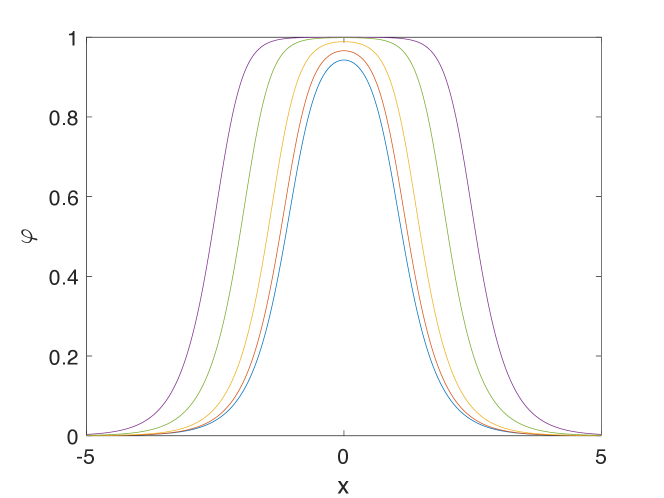
Figure 1. Ground state solution to equation (3) for $\alpha=1$, $a=9$ and $b=4.0$, $4.2$, $4.4$, $4.49$ and $4.499$ (from bottom to top).

For $\alpha=2,3$ we get in the same way the figures in Fig. 2. It can be seen that the higher nonlinearity has a tendency to lead to more compressed peaks as in [1]. But due to the missing scaling invariance of the ground states here, it is difficult to compare them.

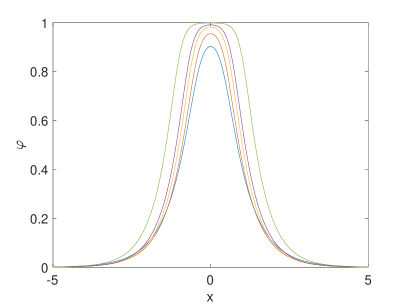
Figure 2. Ground state solution to equation (3) for $a=9$ and $\alpha=2$ on the left ($b=2.0$, $2.5$, $2.8$, $2.9$ and $2.99$ from bottom to top), and for $\alpha=3$ on the right ($b=2.0$, $2.1$, $2.2$, $2.22$ and $2.24$ from bottom to top).

3. Numerical study of the time evolution

In this section we study the time evolution of initial data for the equation (1). We study the stability of the ground state and the time evolution of general initial data in the Schwartz class of smooth rapidly decreasing functions for various parameters.

The results of this section can be summarized in the following

Conjecture 2.

The ground states of equation (1) are asymptotically stable if the perturbed initial data satisfy $|\phi(x,0)|<1$. The long time behavior of solutions for general localized initial data is characterized by ground states and radiation.

Note that the separation of radiation from the bulk is much faster for the cubic case. For higher nonlinearity, this takes considerably longer, and on the used computers, we can reach an agreement of the final state and a ground state of the order of a few percents.

3.1. Time evolution approach

The exponential decay of the stationary solutions makes the use of Fourier spectral methods attractive. Thus we define the standard Fourier transform of a function $u$,

(13) $$\hat{u}=\mathcal{F}u:=\frac{1}{2\pi}\int_{\mathbb{R}}e^{-ikx}u\,dx,\quad k\in\mathbb{R},$$

and consider the $x$-dependence in equation (1) in Fourier space.

The numerical solution is constructed on the interval $x\in L[-\pi,\pi]$ where $L>0$ is chosen such that the solution and relevant derivatives vanish with numerical precision (we work here with double precision which corresponds to an accuracy of the order of $10^{-16}$). The solution $\phi$ is approximated via a truncated Fourier series where the coefficients $\hat{\phi}$ are computed efficiently via a fast Fourier transform (FFT). This means we treat the equation,

(14) $$i\partial_{t}\hat{\phi}=-ik\mathcal{F}\left(\frac{\partial_{x}\phi}{1-|\phi|^{2\alpha}}\right)+\mathcal{F}\left(\alpha|\phi|^{2\alpha-2}\frac{|\partial_{x}\phi|^{2}}{(1-|\phi|^{2\alpha})^{2}}\phi-a|\phi|^{2\alpha}\phi\right),$$

and approximate the Fourier transform in (14) by a discrete Fourier transform.

The study of the solutions to (14) is challenging for several reasons: first it is an NLS equation which leads to a stiff system of ODEs if FFT techniques are used. Since a possible definition of stiffness is that explicit time integration schemes are not efficient, the use of special integrators is recommended in this case. But most of the explicit stiff integrators for NLS equations, see for instance [5] and references therein, assume a stiffness in the linear part of the equations. However, here the second derivatives with respect to $x$ appear in nonlinear terms. Note that the NLS equation is not stiff if perturbations of the ground states are considered, but mainly when zones of rapid modulated oscillations appear, so called dispersive shock waves, see the discussion in [5].

Since we are interested in the former, the main problem of equation (1) is not the stiffness, but the singular term for $|\phi|\to 1$. Since the equation is focusing, it is to be expected that for initial data with modulus close to 1 it will be numerically challenging since the focusing nature of the equation might lead for some time to even higher values of $|\phi|$. Obviously the regime $\phi\sim 1$ is the most interesting from a mathematical point of view since here the strongest deviation from the standard NLS equation is to be expected. To achieve the needed high accuracy for this, a fourth order method is necessary, and even there with small time steps. It turns out that in the studied examples the requirement for accuracy is of similar order as stability conditions for an explicit approach. We apply here the standard explicit fourth order Runge-Kutta method for which the stability condition is $\Delta t\sim 1/N^{2}$, see for instance [9]. We have compared this approach to the unconditionally stable second order Crank-Nicolson method, but had trouble to reach the needed accuracy in an efficient way. The explicit approach is also more efficient than an implicit 4th order Runge-Kutta scheme as applied in [5] where a nonlinear equation has to be solved iteratively at each time step.

The accuracy of the solution is controlled as in [5]: the decrease of the Fourier coefficients indicates the spatial resolution since the numerical error of a truncated Fourier series is of the order of the first neglected Fourier coefficients. The error in the time integration is controlled via conserved quantities. We use the energy (2) which is a conserved quantity of (1), but which will numerically depend on time due to unavoidable numerical errors. In the examples below, the relative energy is always conserved to better than $10^{-6}$.

We test the numerical approach at the example of the ground state. Concretely we consider the ground state solution for $\alpha=1$, $a=9$, $b=4.4$ as initial data. We use $N=2^{10}$ Fourier modes in $x$ for $x\in 5[-\pi,\pi]$ and $N_{t}=10^{5}$ time steps for $t\in[0,1]$. Note that though the ground state solution is stationary, it is not time independent. We compare the numerical and the exact solution, i.e., the solution to (12) times $e^{ibt}$ at the final time $t=1$. This difference is of the order of $10^{-14}$ as shown in Fig. 3. The relative conservation of the energy (2) is during the whole computation of the order of $10^{-14}.$ This shows that the ground state can be numerically evolved with an accuracy of the order $10^{-14}$, and that the conservation of the numerically computed energy indicates the accuracy of the time integration.

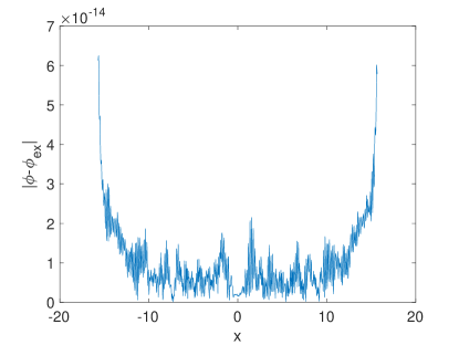
Figure 3. Difference of the numerical solution to the equation (5) for initial data being the ground state solution for $a=9$ and $b=4.4$, and the exact solution for $t=1$.

3.2. Perturbations of ground states

In this subsection we consider the stability of the ground states (12). To this end we perturb it first in the form $\phi(x,0)=\lambda\varphi(x)$, where $\lambda\sim 1$.

Remark 3.

Numerically one cannot consider arbitrary small perturbations as in analytical work since one would have to wait for very large times in order to get meaningful results. But using long times would imply that numerical errors of even high order schemes pile up. Thus in practice one always considers perturbations of the order of $1\%$ (some equations like the Korteweg-de Vries equation allow perturbations of the order of $10\%$ such that the solution stays close to a soliton, and the present equation is similar in this respect). This implies, however, that the final state of a perturbed ground state is not the exact ground state even for asymptotically stable ground states, but a nearby one.

The cubic case

We use $N=2^{11}$ Fourier modes and $N_{t}=5*10^{5}$ time steps for $t\in[0,0.25]$, i.e., more than a whole period of the perturbed ground state. In Fig. 4 we show the solution for the perturbed ground state with $\lambda=0.99$. It can be seen that after a short phase of focusing a ground state with slightly larger maximum than the initial data is reached. In addition there is some radiation towards infinity. The Fourier coefficients of the solution at the final time on the right of Fig. 4 indicate that the solution is fully resolved in $x$.

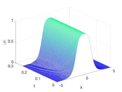
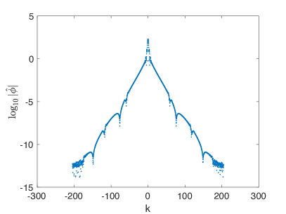
Figure 4. Solution to the equation (5) for the initial data $\phi(x,0)=0.99\varphi(x,a=9,b=4.4)$ and $\alpha=1$ on the left, and the Fourier coefficients of the solution at the final time on the right.

The reaching of a ground state is also suggested by the $L^{\infty}$ norm of the solution shown on the left of Fig. 5. As stated in remark 3, we expect a ground state of slightly different $b$ as the final state since we have a perturbation of the order of $1\%$. To determine this ground state, we use some optimal fitting of the ground state (12) by varying $b$ in order to approximate the solution at the final time. To this end we minimize the residual of the modulus of $\phi$ and $\varphi$ for $|x|<x_{0}$ (we consider $x_{0}=5$) via the optimization algorithm [6] implemented in Matlab as the function fminsearch. On the right of Fig. 5, we show the solution of Fig. 4 at the final time in blue together with a fitted ground state in green. The good agreement (the green curve covers the blue one in the plot where it is identical up to plotting accuracy) shows that the final state is indeed a very nearby ground state, $b=4.388$, which can be already indentified (the difference is of the order of $10^{-3}$) at an early time.

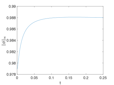
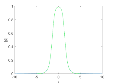
Figure 5. On the left the $L^{\infty}$ norm of the solution of Fig. 4, on the right the solution at the final time in blue and a fitted ground state in green.

If we perturb the same ground state as in Fig. 4 with a factor $\lambda>1$ (such that $||\lambda\varphi||_{\infty}<1$), we observe a similar behavior as can be seen in Fig. 6. The decrease of the modulus of the Fourier coefficients on the right of Fig. 6 indicates that the numerical error in the spatial resolution is of the order of $10^{-8}$. This shows that there are stronger gradients to resolve in this case than in Fig. 4.

Figure 6. Solution to the equation (5) for the initial data $\phi(x,0)=1.001\varphi(x,a=9,b=4.4)$ on the left and the Fourier coefficients of the solution at the final time on the right.

As is more obvious from the $L^{\infty}$ norm in Fig. 7 on the left, a ground state with slightly lower maximum than the initial data is quickly reached. On the right of the same figure we show the solution at the final time in blue together with a fitted ground state ($b=4.4011$) in green. The agreement is so good that the blue line can hardly be seen (the difference is of the order of $10^{-3}$).

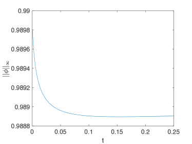
Figure 7. On the left the $L^{\infty}$ norm of the solution of Fig. 4, on the right the solution at the final time in blue and a fitted ground state in green.

The same initial data as above are perturbed with a localized perturbation of the form $\phi(x,0)=\varphi(x)\pm 0.001\exp(-x^{2})$. The resulting $L^{\infty}$ norms of the solutions to (5) for these initial data are shown in Fig. 8. In both cases the $L^{\infty}$ norm appears to approach a slightly smaller ground state than the unperturbed one (for the $-$ sign in the initial data) respectively slightly larger ground state (for the $+$ sign). Note that in the former case, the $L^{\infty}$ norm grows monotonically from its initial value to a value slightly below $0.9888$, whereas it decreases in the latter case monotonically from its initial value to a value slightly above $0.9888$.

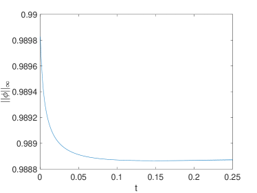
Figure 8. $L^{\infty}$ norms of the solution of (5) for the initial data $\phi(x,0)=\varphi(x)\pm 0.001\exp(-x^{2})$, on the left for the minus sign, on the right for the plus sign in the initial data.

In Fig. 9 we show the solutions for both cases at the final time in blue together with fitted ground states. In both cases the agreement is so good that a difference (again of the order of $10^{-3}$) can hardly be recognized. Thus the ground states appear to be asymptotically stable also in this case. The fitting yields $b=4.3992$ for the $-$ sign and $b=4.4008$ for the $+$ sign, i.e., the expected values close to $4.4$.

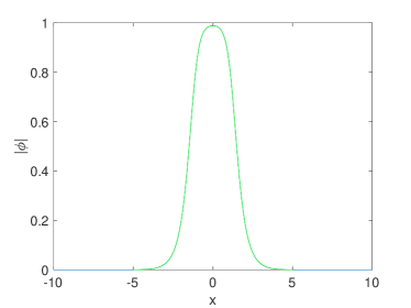
Figure 9. Solutions of (5) for the initial data $\phi(x,0)=\varphi(x)\pm 0.001\exp(-x^{2})$, on the left for the minus sign, on the right for the plus sign in the initial data in blue together with a fitted ground state in green.

Higher nonlinearities

We repeat the experiments of Fig. 4 and Fig. 6 for $\alpha=2$, i.e., a higher nonlinearity. As can be seen below, the ground states still appear to be stable, but take a considerably longer time to settle to a final state. This means we will need much higher numerical resolution in order to avoid too much interaction between the radiation and the bulk on a torus (we simply choose a larger period), and have to solve for longer times. We use $N=2^{13}$ Fourier modes for $x\in 20[-\pi,\pi]$ and $N_{t}=2*10^{6}$ time steps for $t\in[0,2]$.

The $L^{\infty}$ norms for the perturbed ground state can be seen in Fig. 10 on the left. Again a ground state with slightly smaller maximum than the perturbed gound state appears to be reached for $\lambda=0.99$. But this time the $L^{\infty}$ norm performs some damped oscillations around what seems to be an asymptotic value. Since there is no dissipation in the system, this settling into a final state can take quite long compared to a period of the initial ground state, and interestingly takes much longer than in the case $\alpha=1$ above. Note that the quintic nonlinearity is $L^{2}$ critical in the standard NLS equation, i.e., solutions to initial data of sufficient mass blow up in finite time. Here no blow-up is observed, $||\phi||_{\infty}<1$ for all times. The oscillations around some finite value for the $L^{\infty}$ norm can also be seen on the right of Fig. 10, where the solution at the final time is shown together with a ground state of the fitted asymptotic maximum ($b\sim 2.9221$). It can be seen that the fitting is not as good as in the case $\alpha=1$ shown above, and that the found value for $b$ is slightly larger than the original one. This means that the solution at the final time is not yet sufficiently close to the asymptotic solution.

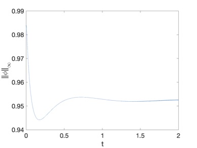
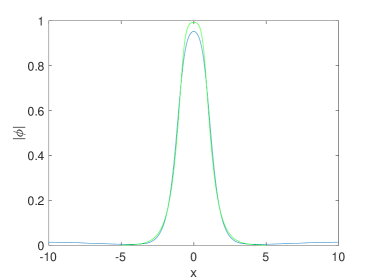
Figure 10. $L^{\infty}$ norm of the solution of (1) for the initial data $\phi(x,0)=\lambda\varphi(x)$ and $a=9$, $b=2.9$ and $\alpha=2$ for $\lambda=0.99$ on the left, on the right the solution at the final time in blue together with an estimated ground state in green.

The situation is very similar for a perturbation with $\lambda=1.001$ shown in Fig. 11. The $L^{\infty}$ on the left of Fig. 11 again appears to oscillate around some asymptotic value which is not fully reached during our computation. A fitted value ($b\sim 2.9315$ for this final state leads to the green curve on the right of the same figure. It shows that the final state is not yet reached, but close to the green curve. Note that the ground state appears to be stable also for the Gaussian perturbations of Fig. 8 which are not shown here.

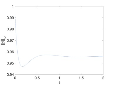
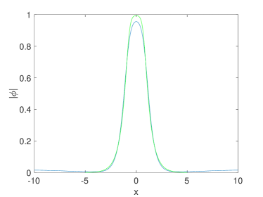
Figure 11. $L^{\infty}$ norm of the solution of (1) for the initial data $\phi(x,0)=\lambda\varphi(x)$ and $a=9$, $b=2.9$ and $\alpha=2$ for $\lambda=1.001$ on the left, on the right the solution at the final time in blue together with an estimated ground state in green.

The same experiments as above are shown for an even higher nonlinearity $\alpha=3$ and $b=2.1$ in Fig. 12 for $\lambda=0.99$. The $L^{\infty}$ norm on the left of the figure appears to oscillate around some some asymptotic value. On the right of the same figure we show the solution at the final time in blue plus a fitted ($b\sim 2.1492$) ground state in green. Once more the ground states appear to be stable (also for Gaussian perturbations not shown here), but the final state will be only fully reached at longer times (the fitted value of $b$ is even larger than the original here).

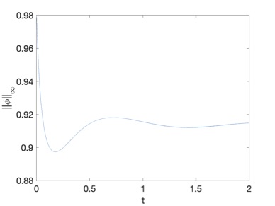
Figure 12. $L^{\infty}$ norm of the solution of (1) for the initial data $\phi(x,0)=0.99\varphi(x)$ and $a=9$, $b=2.1$ and $\alpha=3$ on the left, on the right the solution at the final time in blue together with an estimated ground state in green.

The situation is similar for $\lambda=1.001$ shown in Fig. 13. On the left the $L^{\infty}$ norm appears to oscillate around some asymptotic value. On the right we show the solution at the final time together with a fitted ($b\sim 2.164$) ground state solution in green. Note that for the standard NLS a septic nonlinearity would be $L^{2}$ supercritical which again would lead to a blow-up of initial data of sufficiently large mass.

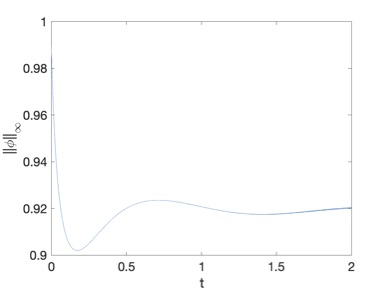
Figure 13. $L^{\infty}$ norm of the solution of (1) for the initial data $\phi(x,0)=1.001\varphi(x)$ and $a=9$, $b=2.1$ and $\alpha=3$ on the left, on the right the solution at the final time in blue together with an estimated ground state in green.

3.3. Schwartz class initial data

An interesting question in this context is whether these stable ground states appear in the long time behavior of solutions to generic localized initial data. To address this question we consider initial data of the form $\phi(x,0)=\mu\exp(-x^{2})$ with $0<\mu<1$, again for $a=9$. We use $N=2^{12}$ Fourier modes for $x\in 40[-\pi,\pi]$ and $N_{t}=5*10^{5}$ time steps for the indicated time intervals. In Fig. 14 it can be seen that the $L^{\infty}$ norm of the solution appears to oscillate around some asymptotic values, and that some radiation is emitted towards infinity.

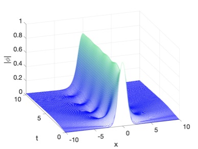
Figure 14. Solution to the equation (5) with $a=9$ for the initial data $\phi(x,0)=0.9\exp(-x^{2})$.

The former effect is more visible on the left of Fig. 15 where the $L^{\infty}$ norm of the solution is shown. Since there is no dissipation in the system, the final ground state will be only reached asymptotically. On the right of the same figure we show the solution at the final time of the computation in blue together with an estimated ground state ($b\sim 2.7188$) in green.

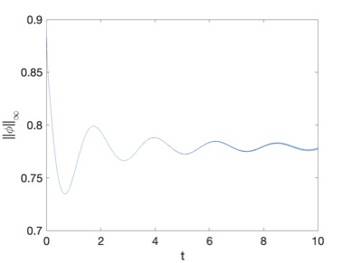
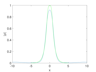
Figure 15. On the left the $L^{\infty}$ norm of the solution of Fig. 14, on the right the solution at the final time in blue together with a fitted ground state in green.

The situation is similar for higher nonlinearity. In Fig. 16 we show the case $\alpha=2$. On the left for $\mu=0.9$, the $L^{\infty}$ norm of the solution appears again to show damped oscillations around some asymptotic value, presumably a ground state. The solution at the final computed time is shown on the right of the same figure together with a fitted ($b=1.4399$) ground state in green. Though the final state is not yet reached, it appears that the soliton resolution conjecture also applies to this case.

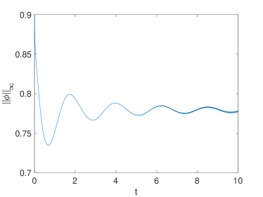
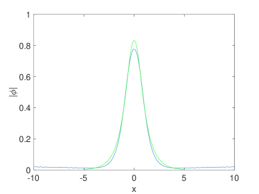
Figure 16. On the left the $L^{\infty}$ norm of the solution of equation (1) for $\alpha=2$ and the initial data $\phi(x,0)=0.9\exp(-x^{2})$, and the solution for $t=10$ on the right in blue together with some fitted ground state in green.

For the even higher nonlinearity $\alpha=3$, we consider in Fig. 17 the case $\mu=0.9$ and show on the left the $L^{\infty}$ norm of the solution which once more shows damped oscillations around some final state. On the right of the same figure we give the solution at the final computed time together with a fitted ground state ($b=1.2549$). Once more the fitting is not perfect since the final state of the solution is not yet reached, but it appears plausible that this final state is indeed a ground state.

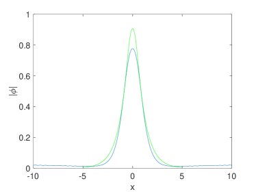
Figure 17. On the left the $L^{\infty}$ norm of the solution of equation (1) for $\alpha=3$ and the initial data $\phi(x,0)=0.9\exp(-x^{2})$, on the right the solution for $t=10$ in blue together with some fitted ground state.

4. Outlook: analysis of the model in higher space dimension

It seems interesting to investigate the model described in this paper in higher space dimension, $d=3$ being the most relevant case from a physical point of view.

On the one hand, to generalize the model for any dimension $d>1$, one can simply replace $\partial_{x}$ in equation (1) by the operator $\nabla$. This leads to a quasilinear Schrödinger equation of the form

$$i\partial_{t}\phi=-\nabla\cdot\left(\frac{\nabla\phi}{1-|\phi|^{2\alpha}}\right)+\alpha|\phi|^{2\alpha-2}\frac{|\nabla\phi|^{2}}{(1-|\phi|^{2\alpha})^{2}}\phi-a|\phi|^{2\alpha}\phi$$

with $\phi\in L^{2}(\mathbb{R}^{d},\mathbb{C})$. On the other hand, at least in dimension $d=2$ and $d=3$, another possibility is to formally derive the equation of the model by following the arguments presented in Appendix A and by taking as starting point the Dirac equation in dimension $1<d\leq 3$. This will lead to a slightly more complicated quasilinear Schrödinger equation.

In both cases, solitary wave solutions for any $\alpha\in\mathbb{N}^{*}$ are expected to exist, and one can investigate their behavior analytically and numerically. However, the study of the time-dependent equation from an analytical point of view seems much more involved.

From a numerical point of view, a stiff time integrator would be recommended for higher dimensions in order to overcome stability constraints, in particular if dispersive shock waves are studied instead of perturbations of ground states as in the present paper. A straightforward, but computationally expensive approach would be an implicit scheme, which probably will have to be combined with some Newton-Krylov scheme since a standard fixed point iteration might not converge except for very small time steps. More interesting would be Rosenbrock-type integrators based on a linearization of the equation after the spatial discretisation, and an exponential integrator for the Jacobian of the resulting system. This can be done efficiently by using so-called Leja points, see for instance [2] and references therein.

We leave this generalization to future work.

Appendix A Formal derivation of the non-relativistic model

Consider the following nonlinear Dirac equation in one space dimension

(15) $$i\partial_{t}\Psi=(-i\sigma_{1}\partial_{x}+\sigma_{3}m)\Psi-\kappa_{1}(\langle\sigma_{3}\Psi,\Psi\rangle)^{\alpha}\sigma_{3}\Psi+\kappa_{2}|\Psi|^{2\alpha}\Psi$$

with $\kappa_{1}$ and $\kappa_{2}$ positive constants and $\alpha\in\mathbb{N}^{*}$. Here $\Psi=(\psi,\zeta)$ is a 2-spinor that describes the quantum state of a nucleon of mass $m$, and $\sigma_{1}$ and $\sigma_{3}$ are the Pauli matrices given by

$$\sigma_{1}=\begin{pmatrix}0&1\\ 1&0\end{pmatrix},\ \sigma_{3}=\begin{pmatrix}1&0\\ 0&-1\end{pmatrix}.$$

In nuclear physics, the interesting regime is when the parameters $\kappa_{1}$ and $\kappa_{2}$ behave like $m$, whereas $\kappa_{1}-\kappa_{2}$ stays bounded. More precisely, let $\kappa_{1}=\theta m$ and $\kappa_{1}-\kappa_{2}=\lambda$ with $\theta$ and $\lambda$ positive constants. As a consequence, the nonlinear Dirac equation (15) can be written as

(16) $$\left\{\begin{aligned} &i\partial_{t}\psi=-i\partial_{x}\zeta+m\psi-\theta m(|\psi|^{2}-|\zeta|^{2})^{\alpha}\psi+(\theta m-\lambda)(|\psi|^{2}+|\zeta|^{2})^{\alpha}\psi,\\ &i\partial_{t}\zeta=-i\partial_{x}\psi-m\zeta+\theta m(|\psi|^{2}-|\zeta|^{2})^{\alpha}\zeta+(\theta m-\lambda)(|\psi|^{2}+|\zeta|^{2})^{\alpha}\zeta.\end{aligned}\right.$$

Hence, by writing

$$\tilde{\phi}(t,x)=e^{imt}\psi(t,x)\text{ and }\tilde{\chi}(t,x)=e^{imt}\zeta(t,x),$$

we obtain

$$\left\{\begin{aligned} &i\partial_{t}\tilde{\phi}=-i\partial_{x}\tilde{\chi}+\theta m\left(\sum_{k=0}^{\alpha}{\alpha\choose k}(|\tilde{\phi}|^{2})^{\alpha-k}|\tilde{\chi}|^{2k}((-1)^{k+1}+1)\right)\tilde{\phi}-\lambda\left(\sum_{k=0}^{\alpha}{\alpha\choose k}(|\tilde{\phi}|^{2})^{\alpha-k}|\tilde{\chi}|^{2k}\right)\tilde{\phi},\\ &i\partial_{t}\tilde{\chi}=-i\partial_{x}\tilde{\phi}-2m\tilde{\chi}+\theta m\left(\sum_{k=0}^{\alpha}{\alpha\choose k}(|\tilde{\phi}|^{2})^{\alpha-k}|\tilde{\chi}|^{2k}((-1)^{k}+1)\right)\tilde{\chi}-\lambda\left(\sum_{k=0}^{\alpha}{\alpha\choose k}(|\tilde{\phi}|^{2})^{\alpha-k}|\tilde{\chi}|^{2k}\right)\tilde{\chi}.\end{aligned}\right.$$

As usual, in the non-relativistic regime, the lower spinor $\tilde{\chi}$ is of order $1/\sqrt{m}$. Hence, we have to perform the following change of scale

$$\tilde{\phi}(t,x)=\left(\frac{1}{\theta}\right)^{\frac{1}{2\alpha}}\phi\left(\frac{t}{2},\sqrt{m}x\right)\text{ and }\tilde{\chi}(t,x)=\left(\frac{1}{\theta}\right)^{\frac{1}{2\alpha}}\frac{1}{2\sqrt{m}}\chi\left(\frac{t}{2},\sqrt{m}x\right)$$

which leads to

$$\left\{\begin{aligned} &i\partial_{t}\phi=-i\partial_{x}\chi+\alpha(|\phi|^{2})^{\alpha-1}|\chi|^{2}\phi-a|\phi|^{2\alpha}\phi+\frac{1}{m}F(1/m,\phi,\chi)\phi\\ &\frac{1}{m}\frac{1}{4}i\partial_{t}\chi=-i\partial_{x}\phi-\chi+|\phi|^{2\alpha}\chi-\frac{1}{m}G(1/m,\phi,\chi)\chi\end{aligned}\right.$$

with $a=\frac{2\lambda}{\theta}$, and $F,G$ defined by

$$F(1/m,\phi,\chi) =2\sum_{k=2}^{\alpha}{\alpha\choose k}(|\phi|^{2})^{\alpha-k}\frac{|\chi|^{2k}}{2^{2k}m^{k-2}}((-1)^{k+1}+1)-a\sum_{k=1}^{\alpha}{\alpha\choose k}(|\phi|^{2})^{\alpha-k}\frac{|\chi|^{2k}}{2^{2k}m^{k-1}},$$

$$G(1/m,\phi,\chi) =\frac{1}{2}\sum_{k=1}^{\alpha}{\alpha\choose k}(|\phi|^{2})^{\alpha-k}\frac{|\chi|^{2k}}{2^{2k}m^{k-1}}((-1)^{k}+1)-\frac{a}{4}\sum_{k=0}^{\alpha}{\alpha\choose k}(|\phi|^{2})^{\alpha-k}\frac{|\chi|^{2k}}{2^{2k}m^{k}}.$$

Finally, denoting $\varepsilon=\frac{1}{m}$ the perturbative parameter, we obtain

(17) $$\left\{\begin{aligned} &i\partial_{t}\phi=-i\partial_{x}\chi+\alpha(|\phi|^{2})^{\alpha-1}|\chi|^{2}\phi-a|\phi|^{2\alpha}\phi+\varepsilon F(\varepsilon,\phi,\chi)\phi,\\ &i\partial_{x}\phi+(1-|\phi|^{2\alpha})\chi+\varepsilon\frac{1}{4}i\partial_{t}\chi+\varepsilon G(\varepsilon,\phi,\chi)\chi=0.\end{aligned}\right.$$

In particular, when $\varepsilon=0$, we have

(18) $$\left\{\begin{aligned} &i\partial_{t}\phi=-i\partial_{x}\chi+\alpha(|\phi|^{2})^{\alpha-1}|\chi|^{2}\phi-a|\phi|^{2\alpha}\phi,\\ &i\partial_{x}\phi+(1-|\phi|^{2\alpha})\chi=0,\end{aligned}\right.$$

which leads at least formally to the time-dependent quasilinear Schrödinger equation

$$i\partial_{t}\phi=-\partial_{x}\left(\frac{\partial_{x}\phi}{1-|\phi|^{2\alpha}}\right)+\alpha(|\phi|^{2})^{\alpha-1}\frac{|\partial_{x}\phi|^{2}}{(1-|\phi|^{2\alpha})^{2}}\phi-a|\phi|^{2\alpha}\phi.$$

Appendix B Existence of positive solutions to the stationary equation (3)

In this appendix, we prove Theorem 1 and we make rigorous the construction of ground states presented in Section 2.

As in [3], we write the stationary equation (3) as a system of first order ODEs

(19) $$\left\{\begin{aligned} &\chi^{\prime}=\alpha\chi^{2}\varphi^{2\alpha-1}-a\varphi^{2\alpha+1}+b\varphi\\ &\varphi^{\prime}=\chi(1-\varphi^{2\alpha})\end{aligned}\right.$$

for any strictly positive integer $\alpha$.

The existence of solutions to (19) is an immediate consequence of the Cauchy-Lipschitz theorem. More precisely, we have the following lemma.

Lemma 4.

Let $\alpha\in\mathbb{N}^{*}$ and $(x_{0},\chi_{0},\varphi_{0})\in\mathbb{R}\times\mathbb{R}^{2}$. For any $a,b>0$, there exist $\gamma>0$ and $(\chi,\varphi)\in\mathcal{C}^{1}([x_{0}-\gamma,x_{0}+\gamma],\mathbb{R}^{2})$ unique solution of (19) satisfying $\chi(x_{0})=\chi_{0}$, $\varphi(x_{0})=\varphi_{0}$. Moreover, $(\chi,\varphi)$ can be extended on a maximal interval $]X_{-},X_{+}[$ for which the following holds

1. either $X_{+}=+\infty$ or $X_{+}<+\infty$ and $\lim_{x\to X_{+}}|\chi|+|\varphi|=+\infty$,

2. either $X_{-}=-\infty$ or $X_{-}>-\infty$ and $\lim_{x\to X_{-}}|\chi|+|\varphi|=+\infty$.

Our goal is then to find an initial condition $(\chi_{0},\varphi_{0})\in\mathbb{R}^{2}$ such that the unique solution of (19) satisfying $\chi(x_{0})=\chi_{0}$, $\varphi(x_{0})=\varphi_{0}$ is defined on $\mathbb{R}$ and $\lim_{x\to\pm\infty}(\chi(x),\varphi(x))=(0,0)$.

A key ingredient of the proof is to remark that system (19) is the Hamiltonian system associated with the energy

(20) $$H(\chi,\varphi)=\frac{1}{2}\chi^{2}(1-\varphi^{2\alpha})+\frac{a}{2(\alpha+1)}\varphi^{2\alpha+2}-\frac{b}{2}\varphi^{2}.$$

As a consequence, to have a complete description of the dynamical system, it is enough to analyze the energy levels of (20), i.e. the curves in the $(\chi,\varphi)$-plane defined by $\Gamma_{c}=\{(\chi,\varphi)|H(\chi,\varphi)=c\}$.

Lemma 5.

[3, for $\alpha=1$] Let $\alpha\in\mathbb{N}^{*}$. For any $a,b>0$, $H$ has the following properties:

1. if $a-b>0$,

   1. $\nabla H(\chi,\varphi)=0$ if and only if $(\chi,\varphi)=(0,0)$, $(\chi,\varphi)=(0,\pm\left(\frac{b}{a}\right)^{1/2\alpha})$, $(\chi,\varphi)=(\pm\sqrt{\frac{a-b}{\alpha}},1)$ or if $(\chi,\varphi)=(\pm\sqrt{\frac{a-b}{\alpha}},-1)$;

   2. $(\chi,\varphi)=(0,\pm\left(\frac{b}{a}\right)^{1/2\alpha})$ are local minima, and $(\chi,\varphi)=(0,0)$, $(\chi,\varphi)=(\pm\sqrt{\frac{a-b}{\alpha}},1)$ and $(\chi,\varphi)=(\pm\sqrt{\frac{a-b}{\alpha}},-1)$ are saddle points of the energy $H$.

2. if $a-b=0$, $\nabla H(\chi,\varphi)=0$ if and only if $(\chi,\varphi)=(0,0)$ or $(\chi,\varphi)=(0,\pm 1)$.

3. if $a-b<0$,

   1. $\nabla H(\chi,\varphi)=0$ if and only if $(\chi,\varphi)=(0,0)$ or $(\chi,\varphi)=(0,\pm\left(\frac{b}{a}\right)^{1/2\alpha})$;

   2. $(\chi,\varphi)=(0,0)$ and $(\chi,\varphi)=(0,\pm\left(\frac{b}{a}\right)^{1/2\alpha})$ are saddle points of the energy $H$.

Remark 6.

Let $\alpha\in\mathbb{N}^{*}$, $a,b>0$ and $(\chi,\varphi)$ a continuous solution of (19), if there exists $x_{0}\in\mathbb{R}$ such that $(\chi(x_{0}),\varphi(x_{0}))=(0,0)$ then $(\chi(x),\varphi(x))\equiv(0,0)$.

Remark 7.

Let $\alpha\in\mathbb{N}^{*}$, $a,b>0$ and $x_{0},\chi_{0}\in\mathbb{R}$. If $(\chi,\varphi)$ is the unique continuous solution of (19) satisfying $\chi(x_{0})=\chi_{0}$, $\varphi(x_{0})=1$ (resp. $\varphi(x_{0})=-1$) then $\varphi(x)\equiv 1$ (resp. $\varphi(x)\equiv-1$).

As a consequence of Remark 7, we have the following lemma.

Lemma 8.

Let $\alpha\in\mathbb{N}^{*}$, $a,b>0$ and $(\chi,\varphi)$ a continuous solution of (19) defined on $\mathbb{R}$ such that $\lim_{x\to\pm\infty}(\chi(x),\varphi(x))=(0,0)$. Then $\varphi^{2}(x)<1$ for all $x\in\mathbb{R}$.

Proof.

Let $(\chi,\varphi)$ a continuous solution of (19) converging to $(0,0)$ as $x\to\pm\infty$. Then $\forall\varepsilon>0$, $\exists\delta_{\varepsilon}>0$ such that $|\varphi(x)|<\varepsilon$ for all $x>\delta_{\varepsilon}$.

Suppose, by contradiction, that there exists $x_{0}\in\mathbb{R}$ such that $\varphi(x_{0})=1$ (resp. $\varphi(x_{0})=-1$). Then Remark 7 implies $\varphi(x)\equiv 1$ (resp. $\varphi(x)\equiv-1$), a contradiction.

∎

Next, since we are interested in solutions of (19) converging to $(0,0)$ as $x\to\pm\infty$, we consider the zero level set of H defined by (20). The curve $\Gamma_{0}=\{(\chi,\varphi)|H(\chi,\varphi)=0\}$ is an algebraic curve of degree $2\alpha+2$ defined by

(21) $$\chi^{2}(1-\varphi^{2\alpha})+\frac{a}{\alpha+1}\varphi^{2\alpha+2}-b\varphi^{2}=0$$

and its behavior depends on the parameters $a$, $b$ and $\alpha$. Moreover in the region $\{(\chi,\varphi)\in\mathbb{R}^{2},\varphi^{2}<1\}$, the equation of $\Gamma_{0}$ can be written as

(22) $$\chi^{2}=\varphi^{2}\frac{b-\frac{a}{\alpha+1}\varphi^{2\alpha}}{1-\varphi^{2\alpha}}.$$

The following two lemmas show the nonexistence of positive solutions of (3) that vanishes at $\pm\infty$ whenever $0<a\leq(\alpha+1)b$.

Lemma 9.

Let $\alpha\in\mathbb{N}^{*}$ and $a,b>0$ such that $a<(\alpha+1)b$. Let $(\chi,\varphi)$ be the solution of (19) satisfying $\chi(x_{0})=\chi_{0}$, $\varphi(x_{0})=\varphi_{0}$. If $(\chi_{0},\varphi_{0})\neq(0,0)$ there is no solution that satisfies $\lim_{x\to\pm\infty}(\chi(x),\varphi(x))=(0,0)$.

Proof.

Since $\varphi$ is a $\mathcal{C}^{1}$ function such that $\lim_{x\to\pm\infty}\varphi(x)=0$, there exits $\tilde{x}\in\mathbb{R}$ such that $\varphi^{\prime}(\tilde{x})=0$. Moreover, thanks to Lemma 8, $\varphi^{2}(\tilde{x})<1$. Hence, since $\varphi$ is a solution to (19), we deduce $\chi(\tilde{x})=0$ that leads to

$$\varphi^{2}(\tilde{x})\frac{b-\frac{a}{\alpha+1}\varphi^{2\alpha}(\tilde{x})}{1-\varphi^{2\alpha}(\tilde{x})}=0$$

using (22).

Now, $\varphi^{2\alpha}(\tilde{x})<1<\frac{(\alpha+1)b}{a}$. Then $\varphi(\tilde{x})=0$ and it follows from Remark (6), that $(\chi(x),\varphi(x))\equiv(0,0)$. This contradicts $(\chi_{0},\varphi_{0})\neq(0,0)$.

∎

Lemma 10.

Let $\alpha\in\mathbb{N}^{*}$ and $a,b>0$ such that $a=(\alpha+1)b$. Let $(\chi,\varphi)$ be the solution of (19) satisfying $\chi(x_{0})=\chi_{0}$, $\varphi(x_{0})=\varphi_{0}$. If $(\chi_{0},\varphi_{0})\neq(0,0)$ there is no solution that satisfies $\lim_{x\to\pm\infty}(\chi(x),\varphi(x))=(0,0)$.

Proof.

If $a=(\alpha+1)b$, the curve $\Gamma_{0}$ is defined as

(23) $$(1-\varphi^{2\alpha})(\chi^{2}-b\varphi^{2})=0$$

and zero contour line is represented in Fig. 18.

Figure 18. $\Gamma_{0}$ when $a=(\alpha+1)b$

Recall that $(\chi(x),\varphi(x))\equiv(0,0)$, $(\chi(x),\varphi(x))\equiv(\pm\sqrt{b},1)$ and $(\chi(x),\varphi(x))\equiv(\pm\sqrt{b},-1)$ are solutions to (19) such that $H(\chi,\varphi)=0$.

Since we are interested in solutions of (19) converging to $(0,0)$ as $x\to\pm\infty$, we can restrict our study to the region $\{(\chi,\varphi)|\varphi^{2}<1\}$. Moreover, because of the symmetries of the problem, it is enough to look for $\varphi\geq 0$. Then, equation (23) implies that $\chi(x)=\sqrt{b}\varphi(x)$ or $\chi(x)=-\sqrt{b}\varphi(x)$. In both cases, the solution $(\chi,\varphi)$ is defined for all $x\in\mathbb{R}$ since $|\varphi|+|\chi|<+\infty$. Finally, since $(\chi,\varphi)$ has to converge to one of the critical points of $H$ as $x$ goes to $\pm\infty$, we can conclude that either

$$\lim_{x\to-\infty}(\chi(x),\varphi(x))=(0,0)\text{ and }\lim_{x\to+\infty}(\chi(x),\varphi(x))=(\sqrt{b},1)$$

or

$$\lim_{x\to-\infty}(\chi(x),\varphi(x))=(-\sqrt{b},1)\text{ and }\lim_{x\to-\infty}(\chi(x),\varphi(x))=(0,0).$$

As a consequence, the unique solution of (19) that satisfies $\lim_{x\to\pm\infty}(\chi(x),\varphi(x))=(0,0)$ is $(\chi(x),\varphi(x))\equiv(0,0)$.

∎

Hence, let $a>(\alpha+1)b$. In this case we are able to prove the existence and uniqueness (modulo translations) of a positive solution $\varphi$ to of (3) such that $\lim_{x\to\pm\infty}\varphi(x)=0$.

Lemma 11.

Let $\alpha\in\mathbb{N}^{*}$ and $a,b>0$ such that $a>(\alpha+1)b$. Then there is a unique (modulo translations) solution $(\chi,\varphi)$ of (19) that satisfies $0<\varphi(x)<1$ for all $x\in\mathbb{R}$ and $\lim_{x\to\pm\infty}(\chi(x),\varphi(x))=(0,0)$. Moreover, there exists $x_{0}\in\mathbb{R}$ such that $\varphi$ is symmetric with respect to $\{x=x_{0}\}$ and strictly decreasing for all $x>x_{0}$.

Proof.

If $(\chi,\varphi)$ is a solution of (19) that satisfies $\varphi(x)>0$ for all $x\in\mathbb{R}$ and $\lim_{x\to\pm\infty}(\chi(x),\varphi(x))=(0,0)$, then there exists $x_{0}\in\mathbb{R}$ such that $\varphi^{\prime}(x_{0})=0$ and $0<\varphi^{2}(x_{0})<1$. Hence, $\chi(x_{0})=0$ and, thanks to (22), $\varphi(x_{0})=\left(\frac{(\alpha+1)b}{a}\right)^{\frac{1}{2\alpha}}<1$.

Let $(\chi_{0},\varphi_{0})=(0,\left(\frac{(\alpha+1)b}{a}\right)^{\frac{1}{2\alpha}})$ and $(\chi,\varphi)$ the unique solution of (19) satisfying $\chi(x_{0})=\chi_{0}$ and $\varphi(x_{0})=\varphi_{0}$. Our goal is to show $\varphi(x)>0$ for all $x\in\mathbb{R}$ and $\lim_{x\to\pm\infty}(\chi(x),\varphi(x))=(0,0)$.

First of all, we show that $(\chi,\varphi)$ is defined for all $x\in\mathbb{R}$. Indeed, let $]X_{-},X_{+}[$ the maximal interval on which the solution $(\chi,\varphi)$ is defined. Thanks to Remark 7, we have $\varphi^{2}(x)<1$ for all $x\in]X_{-},X_{+}[$. This, together with (22) and the fact that $b<\frac{a}{\alpha+1}$, implies $\chi^{2}(x)<\frac{a}{\alpha+1}$ for all $x\in]X_{-},X_{+}[$. As a consequence, $]X_{-},X_{+}[=\mathbb{R}$.

Next, we remark that for any $x>x_{0}$, $\chi(x)<0$. Indeed, equation (19) implies that $\chi^{\prime}(x_{0})=-\alpha b\varphi(x_{0})<0$. Hence, $\chi(x)<0$ for all $x>x_{0}$ sufficiently close to $x_{0}$. Assume, by contradiction, that there is $\tilde{x}\in]x_{0},+\infty[$ such that $\chi(x)<0$ for all $x\in]x_{0},\tilde{x}[$ and $\chi(\tilde{x})=0$. As a consequence, $\varphi^{\prime}(x)<0$ for all $x\in]x_{0},\tilde{x}[$ and

$$\varphi^{2}(\tilde{x})\frac{b-\frac{a}{\alpha+1}\varphi^{2\alpha}(\tilde{x})}{1-\varphi^{2\alpha}(\tilde{x})}=0.$$

This implies $\varphi(\tilde{x})=0$, a contradiction.

With the same argument, we show $\chi(x)>0$ for any $x<x_{0}$ and we conclude that $\varphi(x)>0$ for all $x\in\mathbb{R}$. Moreover, $\varphi$ is strictly decreasing for all $x>x_{0}$ and strictly increasing for all $x<x_{0}$. As a consequence $\max_{x\in\mathbb{R}}\varphi(x)=\varphi(x_{0})=\left(\frac{(\alpha+1)b}{a}\right)^{\frac{1}{2\alpha}}$.

Finally, we know that $(\chi,\varphi)$ has to converge to one of the critical points of $H$ as $x$ goes to $\pm\infty$. On the one hand, the points $(\pm\sqrt{\frac{a-b}{\alpha}},1)$ and $(\pm\sqrt{\frac{a-b}{\alpha}},-1)$ are excluded since $0\leq\lim_{x\to\pm\infty}\varphi(x)\leq\varphi(x_{0})<1$. On the other hand, $H(0,\pm\left(\frac{b}{a}\right)^{1/2\alpha})<0=H(\chi_{0},\varphi_{0})$. Hence $(\chi,\varphi)$ has to converge to $(0,0)$ as $x$ goes to $\pm\infty$.

Next, we have to prove that $\varphi$ is symmetric with respect to $\{x=x_{0}\}$, i.e $\varphi(2x_{0}-x)=\varphi(x)$ for all $x\in\mathbb{R}$. For this, it is enough to remark that $(\chi_{x_{0}}(x),\varphi_{x_{0}}(x)):=(-\chi(2x_{0}-x),\varphi(2x_{0}-x))$ is a solution to (19) that satisfies $\chi_{x_{0}}(x_{0})=0$ and $\varphi_{x_{0}}(x_{0})=\varphi_{0}$. As a consequence $(\chi_{x_{0}}(x),\varphi_{x_{0}}(x))=(\chi(x),\varphi(x))$ for all $x\in\mathbb{R}$.

∎

Remark 12.

As shown in Section 2, a straightforward computation leads to the explicit formula for $\varphi$. In particular, for any fixed $x_{0}\in\mathbb{R}$,

(24) $$\varphi(x)=\left(\frac{1}{2}\left(\frac{a}{(\alpha+1)b}+1\right)+\frac{1}{2}\left(\frac{a}{(\alpha+1)b}-1\right)\cosh({2\alpha\sqrt{b}(x-x_{0})})\right)^{-\frac{1}{2\alpha}}$$

for $x\geq x_{0}$ and $\varphi(x)=\varphi(2x_{0}-x)$ for $x<x_{0}$.

Finally, we conclude by proving the non-degeneracy of the solution $\varphi$. The linearized operator at our solution $\varphi$ is defined by

$$Lv= -\left(\frac{v^{\prime}}{1-\varphi^{2\alpha}}+\left(\frac{\varphi^{\prime}}{1-\varphi^{2\alpha}}\right)\frac{2\alpha\varphi^{2\alpha-1}v}{1-\varphi^{2\alpha}}\right)^{\prime}$$

$$+2\alpha\left(\frac{\varphi^{\prime}}{1-\varphi^{2\alpha}}\right)\varphi^{2\alpha-1}\left(\frac{v^{\prime}}{1-\varphi^{2\alpha}}+\left(\frac{\varphi^{\prime}}{1-\varphi^{2\alpha}}\right)\frac{2\alpha\varphi^{2\alpha-1}v}{1-\varphi^{2\alpha}}\right)$$

(25) $$+\alpha(2\alpha-1)\left(\frac{\varphi^{\prime}}{1-\varphi^{2\alpha}}\right)^{2}\varphi^{2\alpha-2}v-a(2\alpha+1)\varphi^{2\alpha}v+bv.$$

Our goal is to prove that in $L^{2}$, $\ker L=\mathrm{span}\{\varphi^{\prime}\}$.

Lemma 13.

Let $\alpha\in\mathbb{N}^{*}$ and $a,b>0$ such that $a>(\alpha+1)b$ and $\varphi$ the unique solution of (3) that satisfies $0<\varphi(x)<1$ for all $x\in\mathbb{R}$ and $\lim_{x\to\pm\infty}\varphi(x)=0$. Then $\varphi$ is non-degenerate, i.e. $\ker L=\mathrm{span}\{\varphi^{\prime}\}$.

Proof.

First of all, by deriving the equation (3) with respect to $x$, we can easily remark that $\varphi^{\prime}$ is a solution to $Lv=0$. As a consequence $\mathrm{span}\{\varphi^{\prime}\}\subset\ker L$.

Let $v\in\ker L\smallsetminus\mathrm{span}\{\varphi^{\prime}\}$. As a consequence, by writing $u=\frac{v^{\prime}}{1-\varphi^{2\alpha}}+\left(\frac{\varphi^{\prime}}{1-\varphi^{2\alpha}}\right)\frac{2\alpha\varphi^{2\alpha-1}v}{1-\varphi^{2\alpha}}$, we deduce that $v$ is a solution to

(26) $$\left\{\begin{aligned} &u^{\prime}=2\alpha\chi\varphi^{2\alpha-1}u+\alpha(2\alpha-1)\chi^{2}\varphi^{2\alpha-2}v-a(2\alpha+1)\varphi^{2\alpha}v+bv\\ &v^{\prime}=(1-\varphi^{2\alpha})u-2\alpha\chi\varphi^{2\alpha-1}v\end{aligned}\right.$$

with $\chi=\frac{\varphi^{\prime}}{1-\varphi^{2\alpha}}$. Note that (26) is simply the linearization of (19) at the solution $(\chi,\varphi)$, $(\chi^{\prime},\varphi^{\prime})$ is a solution to (26) and the non-degeneracy property will follow from the fact $(0,0)$ is a non-degenerate minimum of $H$. More precisely, a direct computation, using the fact that $(u,v)$ and $(\chi^{\prime},\varphi^{\prime})$ are solutions to (26), gives $(u\varphi^{\prime}-v\chi^{\prime})^{\prime}=0$. Hence, the function $u\varphi^{\prime}-v\chi^{\prime}$ is constant and in particular $u(x)\varphi^{\prime}(x)-v(x)\chi^{\prime}(x)=u(x_{0})\varphi^{\prime}(x_{0})-v(x_{0})\chi^{\prime}(x_{0})=-v(x_{0})\chi^{\prime}(x_{0})$ with $x_{0}$ defined as in the proof of Lemma 11 so that $\chi^{\prime}(x_{0})=-\alpha b\varphi(x_{0})<0$. If $v(x_{0})=0$, then $u\varphi^{\prime}-v\chi^{\prime}\equiv 0$ and using the definition of $u$ we can conclude $v\equiv 0$. If $v(x_{0})>0$ (resp. $v(x_{0})<0$), then $u(x)\varphi^{\prime}(x)-v(x)\chi^{\prime}(x)=\alpha b\varphi(x_{0})v(x_{0})>0$ (resp. $u(x)\varphi^{\prime}(x)-v(x)\chi^{\prime}(x)=\alpha b\varphi(x_{0})v(x_{0})<0$) and $(u,v)$ cannot converge to $(0,0)$ as $x$ goes to $\pm\infty$. Hence, $v\notin\ker L$.

∎

References

- [1] J. Arbunich, C. Klein and C. Sparber, On a class of derivative Nonlinear Schrödinger-type equations in two spatial dimensions, M2AN, 53 (5), 1477–1505, (2019).
- [2] M. Caliari, P. Kandolf, A. Ostermann and S. Rainer, The Leja method revisited: backward error analysis for the matrix exponential, SIAM J. SCI. COMPUT., 38 (3), pp. A1639ÐA1661
- [3] M. J. Esteban and S. Rota Nodari, Symmetric ground states for a stationary relativistic mean-field model for nucleons in the nonrelativistic limit, Rev. Math. Phys., 24 (2012), pp. 1250025–1250055.
- [4] M. J. Esteban and S. Rota Nodari, Ground states for a stationary mean-field model for a nucleon, Ann. Henri Poincaré, 14 (2013), pp. 1287–1303.
- [5] C. Klein, Fourth order time-stepping for low dispersion Korteweg-de Vries and nonlinear Schrödinger equation, ETNA, 29, 116-135, (2008).
- [6] J.C. Lagarias, J.A. Reeds, M.H. Wright, and P.E. Wright, Convergence properties of the NelderÐMead simplex method in low dimensionsn SIAM J. Optim., 9, 112Ð147 (1988).
- [7] M. Lewin and S. Rota Nodari, Uniqueness and non-degeneracy for a nuclear nonlinear Schrödinger equation, Nonlinear Differ. Equ. Appl. (NoDEA), 22 (2015), pp. 673–698.
- [8] C. Sulem and P.L. Sulem, The nonlinear Schrödinger equation: self-focusing and wave collapse. Springer Ser. Appl. Math. Sci. Springer, Berlin 139 (1999).
- [9] L. N. Trefethen, Spectral Methods in Matlab, SIAM, Philadelphia, PA, 2000.
- [10] L. Le Treust and S. Rota Nodari, Symmetric excited states for a mean-field model for a nucleon, Journal of Differential Equations, 255 (2013), pp. 3536–3563.