Shortcuts to adiabaticity for an interacting Bose-Einstein condensate via exact solutions of the generalized Ermakov equation

Abstract

Shortcuts to adiabatic expansion of the effectively one-dimensional Bose-Einstein condensate (BEC) loaded in the harmonic-oscillator (HO) trap is investigated by combining techniques of the variational approximation and inverse engineering. Piecewise-constant (discontinuous) intermediate trap frequencies, similar to the known bang-bang forms in the optimal-control theory, are derived from an exact solution of a generalized Ermakov equation. Control schemes considered in the paper include imaginary trap frequencies at short time scales, i.e., the HO potential replaced by the quadratic repulsive one. Taking into regard the BEC’s intrinsic nonlinearity, results are reported for the minimal transfer time, excitation energy (which measures deviation from the effective adiabaticity), and stability for the shortcut-to-adiabaticity protocols. These results are not only useful for the realization of fast frictionless cooling, but also help to address fundamental problems of the quantum speed limit and thermodynamics.

Tang-You Huang

Boris A. Malomed

Xi Chen

"Shortcuts to adiabaticity" (STA) for efficient transformation of trapped nonlinear-wave modes are important tools which help to improve quality of the transformation, simultaneously optimizing its efficiency. In this work, we focus on the shortcuts for expansion of effectively one-dimensional Bose-Einstein condensates (BECs), described by the Gross-Pitaevskii equation (GPE) including the cubic self-interaction of the wave function and the harmonic-oscillator (HO) trapping potential with a time-dependent strength. We design simple but fast STA protocols, using the method of inverse engineering, realized by means of the variational approximation applied to the GPE. A generalized Ermakov equation, including an additional term induced by the self-interaction of the BEC, is thus derived (the classical second-order ordinary differential equation of this type was derived and solved by Russian mathematician Ermakov about 150 years ago). Results of the analysis help us to elaborate schemes for the time modulation of the HO-trap frequency, admitting fast frictionless cooling of the expanding BEC in the weak-interaction regime. In particular, the schemes based on the “bang" and “bang-bang" forms, which are well known in the optimal-control theory, are exemplified. The minimal transformation time, time-averaged energy of excitations generated around the expanding state, and stability of the dynamical regimes with attractive and repulsive self-interactions are analyzed for various STA protocols. In addition to direct applications to the expansion (or compression) of BEC, the results are relevant for studies of the quantum speed limit and manifestations of the third principle of thermodynamics in quantum systems in general.

I Introduction

Precise control and manipulations of non-interacting and interacting Bose-Einstein condensates (BECs) in trapping potentials has well-known significance to applications ranging from quantum simulations, information processing, and quantum-enhanced metrology to atom interferometry Cohen-Tannoudji and Guéry-Odelin (2011). A particularly relevant example is the transfer a quantum system from the ground state of one potential into that of another, through its evolution governed by a specifically designed Hamiltonian. To this end, slow adiabatic processes Kastberg et al. (1995), as well as fast shortcuts through intermediate states Anderson et al. (1994), Fourier transform Couvert et al. (2008), optimal control Bulatov et al. (1998, 1999); Salamon et al. (2009), and machine learning Henson et al. (2018) have been exploited for the realization of fast frictionless cooling and transport of cold atoms, trapped ions, and BEC in magneto-optical traps, and high-quality compression of optical solitons Anderson et al. (1994).

As concerns the concept of “shortcuts to adiabaticity" (STA), it has recently drawn much interest to speed up slow adiabatic processes, while suppressing the excitation or heating, with important applications to atomic, molecular, optical and statistical physics, see reviews Torrontegui et al. (2013); Guéry-Odelin et al. (2019); del Campo and Kim (2019). In this context, a series of works were devoted to frictionless expansion/compression and cooling of atomic Bose-Einstein condensates (BECs) in time-modulated harmonic-oscillator (HO) traps Muga et al. (2009); Chen et al. (2010); Schaff et al. (2010, 2011a); Del Campo (2011); Schaff et al. (2011b) , with extensions to cold-atom mixtures Choi et al. (2011), Tonks-Girardeau (TG) del Campo (2011); Deffner et al. (2014) and Fermi Papoular and Stringari (2015); Deng et al. (2018) gases, and many-body systems Guéry-Odelin et al. (2014); Rohringer et al. (2015). These results are not only significant for the design of optimal quantum control Rezek et al. (2009); Stefanatos et al. (2010), but also have significant implications for the studies of quantum speed limits, in the context of the trade-off between time and energy cost under the constraint of the third law in quantum thermodynamics Hoffmann et al. (2011); Chen and Muga (2010). Other systems, such as mechanical resonators Li et al. (2011), photonic lattices Stefanatos (2014), bosonic Josephson junction Juliá-Díaz et al. (2012); Yuste et al. (2013); Stefanatos and Paspalakis (2018); Hatomura (2018) , Brownian particles Martínez et al. (2016) and classical RC circuits Faure et al. (2019) have been extensively studied by using similar STA techniques for the swift transformation between two adiabatic or equilibrium states.

Theoretically, the STA techniques, among which the most popular ones are inverse engineering Chen et al. (2010), counter-diabatic driving Berry (2009); Deffner et al. (2014); del Campo (2013) and fast-forward scaling Masuda and Nakamura (2008); Torrontegui et al. (2012a), which were elaborated in different setups, although they are mathematically equivalent Torrontegui et al. (2012a); Chen et al. (2011). In the contexts of the inverse engineering, Lewis-Riesenfeld dynamical invariant Chen et al. (2010), or general scaling transformations Castin and Dum (1996); Gritsev et al. (2010), various forms of the famous Ermakov equation Ermakov (1880); Lewis (1967); Reid and Ray (1980); Ray (1980); Rogers and Schief (2018); C. Rogers and Malomed (2020) were derived for designing shortcuts to adiabatic expansions of non-interacting thermal gases and BEC in the Thomas-Fermi (TF) regime Muga et al. (2009); Schaff et al. (2011a); Del Campo (2011); Schaff et al. (2011b). Specifically, when it comes to the shortcuts for BECs, the TF regime Muga et al. (2009); Schaff et al. (2011b) or time-dependent nonlinear coupling Muga et al. (2009) lead to (modified) Ermakov equations, starting from the Gross-Pitaevskii (GP) equation, which is the commonly adopted dynamical model of BEC in the mean-field theory Pitaevskii and Stringari (2003).

In this work, inspired by approaches based on the variational approximation (VA) Pérez-García et al. (1996); García-Ripoll et al. (1999), similar to those developed in nonlinear optics Anderson et al. (1994); Malomed (2002), we derive a generalized Ermakov equation, including a term induced by the self-interaction term in the GP equation. The objective is to further elaborate shortcuts for the adiabatic expansion/compression in BEC. This allows us to manipulate nonlinear dynamics of BEC solitons by means of the Feshbach resonance Li et al. (2016, 2018) and many-body dynamics in power-law potentials Xu et al. (2020). In particular, we exploit the VA to design shortcuts to adiabaticity for the decompression of BEC in HO traps. Exact solutions to the generalized Ermakov equation, including bang and bang-bang control scenarios, are analytically obtained and used to highlight the effect of inter-atomic interactions on the minimal time and stability of the BEC manipulations. The results for the time-optimal driving are different from those previously obtained for single atoms Chen and Muga (2010); Stefanatos et al. (2010); Rezek et al. (2009) and BEC in the TF limit Stefanatos and Li (2012), where negligible or very strong interactions are assumed.

II The model, Hamiltonian, and variational approach

We begin with the effective one-dimensional (1D) GP equation, modeling the mean-field dynamics of the cigar-shaped BEC Salasnich et al. (2002):

$$i\frac{\partial\psi}{\partial t}=-\frac{1}{2}\frac{\partial^{2}\psi}{\partial x^{2}}+\frac{1}{2}\omega^{2}(t)x^{2}\psi+gN|\psi|^{2}\psi,$$ (1)

where $\omega(t)$ is time-dependent trapping frequency, $g$ is the nonlinearity coefficient representing atom-atom interaction, and $N$ is the total number of atoms. The scaled variables are related to their counterparts measured in physical units (with tildes) as per $t=\omega_{0}\tilde{t}$, $\omega(t)=\tilde{\omega}(t)/\omega_{0}$, $x=\tilde{x}/\sigma_{0}$, $g=\tilde{g}/\hbar\omega_{0}\sigma_{0}$, where $m$ is atomic mass, $\omega_{0}$ is the initial longitudinal trapping frequency, $\sigma_{0}=\sqrt{\hbar/m\omega_{0}}$ is the corresponding cloud size, $\tilde{g}=2\hbar a_{s}\omega_{\perp}$ with scattering length $a_{s}$ and the trapping frequency of the transverse potential, $\omega_{\perp}$, which provides for reduction of the underlying three-dimensional GP equation to the 1D form (1), provided that $\omega_{\perp}$ is much larger than the one acting in the axial direction. Further, if the axial HO potential is time-dependent, the use of the 1D equation (1) is fully justified if the respective frequencies of the time dependence are much smaller than $\omega_{\perp}$.

In order to apply the VA Pérez-García et al. (1996); García-Ripoll et al. (1999), we start with the Lagrangian density of Eq. (1),

$$\mathscr{L} = \frac{i}{2}\left(\psi\frac{\partial\psi^{\ast}}{\partial t}-\psi^{\ast}\frac{\partial\psi}{\partial t}\right)-\frac{1}{2}\left|\frac{\partial\psi}{\partial x}\right|^{2}$$ (2)

$$-\frac{1}{2}\omega^{2}(t)x^{2}|\psi|^{2}-\frac{1}{2}gN|\psi|^{4}.$$

Plugging the usual time-dependent Gaussian ansatz,

$$\psi(x,t)=A(t)\exp\left[-\frac{x^{2}}{2a^{2}(t)}+ib(t)x^{2}\right],$$ (3)

in Eq. (2), we calculate the effective Lagrangian $L=\int_{-\infty}^{+\infty}\mathscr{L}[\psi]dx$. Here $a(t)$ and $b(t)\$ represent the width and chirp of the wave function, and amplitude $A(t)=(1/\pi a^{2})^{1/4}$ is the amplitude of wave function, determined by the normalization condition, $\int_{-\infty}^{+\infty}\left|\psi(x)\right|^{2}dx=1$. The variational procedure applied to the Lagrangian makes it possible to eliminate the chirp, $b=-\dot{a}/2a$, the resulting Euler-Lagrange equation for $a(t)$ taking the form of the generalized Ermakov equation Quinn and Haque (2014):

$$\ddot{a}+\omega^{2}(t)a=\frac{1}{a^{3}}+\frac{gN}{\sqrt{2\pi}a^{2}},$$ (4)

which is tantamount to the Newton’s equation of motion for a particle with unit mass, $\ddot{a}=-dU(a)/da$ (with the overdot standing for the time derivative), with the effective potential and the corresponding energy,

$$U(a) = \frac{1}{2}{\omega}^{2}(t)a^{2}+\frac{1}{2a^{2}}+\frac{gN}{\sqrt{2\pi}a},$$ (5)

$$\mathcal{E}(a) = \frac{\dot{a}^{2}}{2}+\frac{1}{2}{\omega}^{2}(t)a^{2}+\frac{1}{2a^{2}}+\frac{gN}{\sqrt{2\pi}a}.$$ (6)

The presence of term $\sim gN$ in Eq. (4) makes it different from the original Ermakov equation,

$$\ddot{a}+\omega^{2}(t)a=\frac{1}{a^{3}},$$ (7)

derived from the Lewis-Reseifiend invariant Chen et al. (2010) or by means of the scaling transform Castin and Dum (1996); Gritsev et al. (2010), see also Appendix A.

III Shortcuts to adiabaticity

In this section, we aim to construct STA protocols of time-dependent trapping by selecting an appropriate time-dependent frequency in Eq. (4), to guarantee a fast transform from the ground state at time $t=0$ to another ground state at a fixed final time, $t=t_{f}$ , avoiding additional (unwanted) excitations. The initial value is taken as $\omega(0)=1$, and the final one is defined as $\omega(t_{f})=1/\gamma^{2}$ , i.e., $\gamma\equiv\sqrt{\omega_{0}/\omega_{f}}$ may be considered an appropriate control parameter. To guarantee that the initial and final states are stationary ones, one has to impose the following boundary conditions:

$$a(0) = a_{\mathrm{i}},~{}~{}a(t_{f})=a_{\mathrm{f}},$$ (8)

$$\dot{a}(0) = \dot{a}(t_{f})=0,$$ (9)

$$\ddot{a}(0) = \ddot{a}(t_{f})=0,$$ (10)

where $a_{\mathrm{i}}$ and $a_{\mathrm{f}}$ are unique positive real solutions of equations

$$a_{\mathrm{i}}^{4}-\frac{gN}{\sqrt{2\pi}}a_{\mathrm{i}} = 1,$$ (11)

$$\frac{a_{\mathrm{f}}^{4}}{\gamma^{4}}-\frac{gN}{\sqrt{2\pi}}a_{\mathrm{f}} = 1,$$ (12)

which follow from the generalized Ermakov equation (4) with $\ddot{a}(0)=\ddot{a}(t_{f})=0$. Clearly, $a_{\mathrm{i}}=1$ and $a_{\mathrm{f}}=\gamma$ in the limit $gN\rightarrow 0$. Therefore, by analogy to the perturbative Kepler problem, the boundary conditions defined by Eqs. (8)-(10) imply minimization of the effective potential $U(a)$ (5), as well as of the energy given by Eq. (6) without the kinetic-energy term.

III.1 Inverse engineering

Here we address an example of atomic cooling by decompressing from initial frequency $\omega_{0}=250\times 2\pi$ Hz to the final one $\omega_{f}=2.5\times 2\pi$ Hz. In the linear limit, $gN\rightarrow 0$, the values are $a_{\mathrm{i}}=1$ and $a_{\mathrm{f}}=\gamma=10$. However, due to the atom-atom interaction, the initial and final sizes of the BEC cloud are slightly different, $a_{\mathrm{i}}=1.001$ and $a_{\mathrm{f}}=10.099$ , as calculated numerically from Eqs. (11) and (12) with the nonlinearity strength $gN$. The boundary conditions being fixed, trajectory of $a(t)$ may be approximated by the simplest polynomial ansatz Chen et al. (2010),

$$a(t)=a_{\mathrm{i}}-6(a_{\mathrm{i}}-a_{\mathrm{f}})s^{5}+15(a_{\mathrm{i}}-a_{\mathrm{f}})s^{4}-10(a_{\mathrm{i}}-a_{\mathrm{f}})s^{3},$$ (13)

with $s=t/t_{f}$. As a consequence, smooth function $\omega(t)$ may be inversely determined by Eq. (4). If an imaginary trap frequency is dealt with, which corresponds to a parabolic repeller, instead of the HO trap, in Eq. (1), $t_{f}$ may be formally made arbitrarily short. However, physical constraints always exist in practice, see the discussion below. Generally, the use of the switch between the trapping and expulsive potentials extends possibilities for the design of control schemes with diverse functionalities.

Here we chose $t_{f}=5.45$, such that the absolute value of the real frequency is bounded by $\omega_{0}$ ($\omega_{0}<\omega_{f}$). Figure 1 illustrates the respective time-varying trap frequency and evolution of the width, as produced by the inverse-engineering method, where the initial and final trap frequencies are $\omega(0)=1$ and $\omega(t_{f})=1/\gamma^{2}$ , and $gN=0.01$. Later, we will compare such smooth trajectories with results produced by the so-called bang and bang-bang control, which is relevant for the time-optimal solution, implemented by means of piecewise-constant (discontinuous) intermediate trap frequencies.

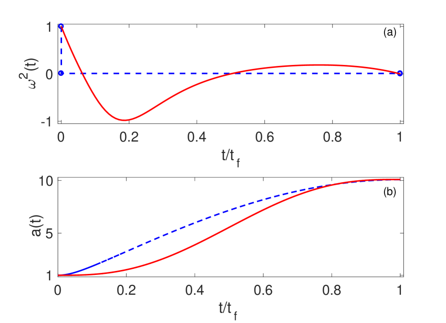
Figure 1: The time dependence of the designed trap frequency, $\omega(t)$ (a), and width of the wave packet (b). Red solid and blue dashed lines correspond to the inverse engineering and bang control, respectively. The parameters are $\omega(0)=1$, $\omega(t_{f})=1/\gamma^{2}$, $gN=0.01$. Note that $t_{f}=5.45$ for the inverse engineering is different $t_{f}=15.83$ for 2-jump control.

III.2 The two-jump control

In the limit of $gN\rightarrow 0$, a simple exact solution of the Ermakov equation can be constructed, that reproduces the shortcut with just one intermediate frequency Chen and Muga (2010), similar to the scenario for the compression of solitons in nonlinear fibers, by passing the soliton from a fiber segment with a large dispersion coefficient to a segment with is a smaller one. This scenario was theoretically elaborated in Ref. Anderson et al. (1994) and experimentally realized in Barak et al. (2008). Motivated by this, we assume that, at $t=0$, the trap frequency suddenly changes from $\omega(0)$ to some constant intermediate value $\omega_{c}$, to achieve an alternative shortcut.

In the linear limit, $gN\rightarrow 0$, the trap frequency remains equal to $\omega_{c}$, from $t=0$ to

$$t_{f}=\pi/\left(2\omega_{c}\right),$$ (14)

and at moment $t=t_{f}$ the frequency instantaneously changes from $\omega_{c}$ to the final value, $\omega(t_{f})$. The exact solution of the Ermakov equation (7) with constant $\omega_{c}$ is well known:

$$a^{2}(t)=\frac{1}{2}\left[\left(A+C\right)+\left(A-C\right)\cos\left(2\omega_{c}t\right)\right],$$ (15)

with constants $A$ and $C$ subject to constraint $AC=1/\omega_{c}^{2}$. To secure the transformation of a stationary state taken at $t=0$ into another stationary one at $t=t_{f}$, it is necessary to impose the above-mentioned conditions, $a(0)=1$, $a(t_{f})=\gamma$, and $\dot{a}(0)=\dot{a}(t_{f})=0$. After a straightforward algebra, the combination of such conditions and Eq. ( 15) yields a simple solution:

$$a(t)=\sqrt{1+\frac{1-\omega_{c}^{2}}{\omega_{c}^{2}}\sinh^{2}(\omega_{c}t)},$$ (16)

with

$$\omega_{c}=\sqrt{\omega(0)\omega(t_{f})}=1/\gamma.$$ (17)

Thus, Eqs. (14) and (16) provide a simple exact solution for the shortcut if the nonlinearity is negligible. In particular, the necessary intermediate trapping frequency $\omega_{c}$ is given as the geometric mean of the initial and final frequencies.

The solution can be generalized for full equation (4), although in a less explicit form. The shortcut scenario implies that the initial and final values (8), subject to boundary conditions (9), are coupled by the motion in potential (5). The energy conservation in this mechanical (perturbative Kepler) problem implies $U(a_{\mathrm{i}})=U(a_{\mathrm{f}})$, or, in an explicit form,

$$\omega_{c}^{2}=\frac{1}{a_{\mathrm{i}}^{2}a_{\mathrm{f}}^{2}}+\sqrt{\frac{2}{\pi}}\frac{gN}{a_{\mathrm{i}}a_{\mathrm{f}}(a_{\mathrm{i}}+a_{\mathrm{f}})}.$$ (18)

In this case, a simple expression for $t_{f}$ is not available, but it can be written in the form of an integral:

$$t_{f}=\int_{a_{\mathrm{i}}}^{a_{\mathrm{f}}}\frac{da}{\sqrt{2\left[U(a_{\mathrm{in}})-U(a)\right]}},$$ (19)

where $a_{\mathrm{i}}$ and $a_{\mathrm{f}}$ are given by Eq. (8). Thus, the trap frequency $\omega(t)$ and trajectory for $a(t)$ can be obtained in a numerical form from Eq. (4) with boundary conditions, see Fig. 1, where $\omega_{c}=0.0993$ and $t_{f}=15.83$ are obtained for the chosen parameters, $\omega(0)=1$, $\omega(t_{f})=1/\gamma^{2}$, and $gN=0.01$. Most importantly, the designed trajectory $a(t)$ satisfies the boundary conditions (8) and (9), which guarantees the realization of the STA protocol and secures the stability at $t>t_{f}$. However, since the boundary condition (10), for the second derivative of $a(t)$, is not fulfilled, one has to design the trap frequency suddenly change. Namely, the trap frequency has to “jump” from initial value $\omega_{0}$ to intermediate one $\omega_{c}$ at $t=0$, and “jump” back to final one $\omega_{f}$ at $t=t_{f}$.

III.3 The three-jump bang-bang control

Next, we address the generalized Ermakov equation (4) and discuss the time-minimization optimal-control problem with a constrained trap frequency, that is, $|\omega(t)|^{2}\leq\delta$. To follow the usual conventions adopted in the optimal control theory, we set new notation,

$$x_{1}\equiv a,~{}~{}x_{2}\equiv\dot{a},$$ (20)

$u(t)\equiv\omega^{2}(t)$, and rewrite Eq. (4) as a system of the first-order differential equations:

$$\dot{x}_{1} = x_{2},$$ (21)

$$\dot{x}_{2} = -ux_{1}+\frac{1}{x_{1}^{3}}+\frac{gN}{\sqrt{2\pi}}\frac{1}{x_{1}^{2}},$$ (22)

where $x_{1}$, $x_{2}$ are the components of a “state vector" $\mathbf{x}$, and squared trap frequency $u(t)$ is considered as a (scalar) control function. The form of the theoretical time-optimal solution can be found using the Pontryagin’s maximum principle, which provides necessary conditions for the optimality. Similar to the approach used in Refs. Stefanatos et al. (2010); Stefanatos and Li (2012), determining the optimal frequency profile reduces to finding $u(t)$ subject to the bound $|u(t)|\leq\delta$ with $u(0)=1$ and $u(t_{f})=1/\gamma^{2}$, such that the above system starts with initial conditions $(x_{1}(0),x_{2}(0))=(a_{\mathrm{i}},0)$, and reaches the final point $(x_{1}(t_{f})$, $x_{2}(t_{f}))=(a_{\mathrm{f}},0)$ in minimal time $t_{f}$. The boundary conditions for $x_{1}$ and $x_{2}$ may be equivalently considered as those for $a$ and $\dot{a}$, see Eqs. ( 8) and (9). The boundary conditions for $u(t)$ are equivalent to those for $\omega(t)$ and, through Eq. (4) or Eqs. (11) and (12), equivalent to those for $\ddot{a}$, hence there are, totally, six boundary conditions, as in Eqs. (8-10).

To find the minimal time $t_{f}$, we define the cost function,

$$J=\int_{0}^{t_{f}}dt=t_{f}.$$ (23)

The control Hamiltonian $H_{c}(\mathbf{p},\mathbf{x},u)$ is

$$H_{c}(\mathbf{p},\mathbf{x},u)=p_{0}+p_{1}x_{2}-p_{2}x_{1}u+\frac{p_{2}}{x_{1}^{3}}+\frac{gN}{\sqrt{2\pi}}\frac{p_{2}}{x_{1}^{2}},$$ (24)

where vector $\mathbf{p}=(p_{0},p_{1},p_{2})$ is composed of non-zero and continuous Lagrange multipliers, $p_{0}<0$ may be chosen for convenience, as it amounts to multiplying the cost function by a constant, and $p_{1,2}$ obey the Hamilton’s equations: $\dot{\mathbf{x}}=\partial H_{c}/\partial\mathbf{x}$ and $\dot{\mathbf{p}}=-\partial H_{c}/\partial\mathbf{x}$. For almost all $0\leq t\leq t_{f}$, function $H_{c}(\mathbf{p},\mathbf{x},u)$ attains its maximum at $u=u(t)$, and $H_{c}(\mathbf{p},\mathbf{x},u)$ is a constant. Making use of the Hamiltonian’s equation, we arrive at the following explicit expressions:

$$\dot{p}_{1} = p_{2}\left(u+\frac{3}{x_{1}^{4}}+\frac{2gN}{\sqrt{2\pi}}\frac{1}{x_{1}^{3}}\right),$$ (25)

$$\dot{p}_{2} = -p_{1}.$$ (26)

It is clear that the control Hamiltonian $H_{c}(\mathbf{p},\mathbf{x},u)$ is a linear function of variable $u(t)$. Therefore, the maximization of $H_{c}(\mathbf{p},\mathbf{x},u)$ is determined by the sign of term $-up_{2}x_{1}$, which, in turn, is determined by the sign of $p_{2}$, as $a(t)$ is always positive, i.e., $x_{1}>0$ and $p_{2}\not=0$. Here $p_{2}=0$ does not provide singular control, and only takes place at specific moments (switching times). As a consequence, we arrive at the scheme of the “bang-bang" control, defined by the following form:

$$u(t)=\begin{cases}-\delta,\qquad p_{2}>0,\\ ~{}\delta,~{}\qquad p_{2}<0,\end{cases}$$ (27)

which implies that the controller switches from one boundary value to the other at the switching times. When $u$ is constant and Eq. (4) holds, then it can be derived that

$$x_{2}^{2}+ux_{1}^{2}+\frac{1}{x_{1}^{2}}+\frac{2gN}{\sqrt{2\pi}x_{1}}=c,$$ (28)

where $c$ is an integration constant. Moreover, we see from Eq. (6) that trajectories with constant $u$ correspond to constant energy $\mathcal{E}(a)=c/2$.

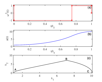
Figure 2: Controller $u$ for “bang-bang" scheme with one intermediate switch (a), the width $a$ of the wave packet (b), and the corresponding trajectory (c). Parameters: $\delta=1$ and others are the same as those in Fig. 1.

By choosing the simplest but feasible “bang-bang" control with only one intermediate switching at $t=t_{1}$, we introduce the three-jumps form,

$$u(t)=\begin{cases}1\qquad~{}~{}~{}~{}~{}t=0,\\ -\delta,\qquad~{}~{}0<t<t_{1},\\ \delta,~{}~{}\qquad~{}~{}t_{1}<t<t_{2},\\ 1/\gamma^{2}\qquad~{}t=t_{f}=t_{1}+t_{2},\end{cases}$$ (29)

as shown in Fig. 2(a), where we take $\delta=1$ as an example, and other parameters are the same as in Fig. 1. Obviously, the discontinuities at the time edges are not implied by the maximum principle, but are determined by the initial and final conditions imposed on control $u$ . This guarantees the creation of the STA protocol, but requires the sudden change of the trap frequencies. Therefore, we can find a lower bound on the minimum time, achieved only with instantaneous jumps of the control at the initial and final times.

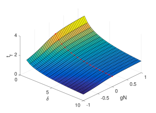
Figure 3: The dependence of minimal time $t_{f}$ on bound $\delta$ of the trap frequency and nonlinearity $gN$, other parameters being the same as in Fig. 1. The red dashed line indicates the minimal time predicted by the optimal-control theory for $gN=0$.

Next, we aim to calculate the necessary time for the transfer from the initial point, $A(a_{\mathrm{i}},0)$, to the final one, $C(a_{\mathrm{f}},0)$ , as shown in Fig. 2(c), where $B(x_{1}^{B},x_{2}^{B})$ is the intermediate point at the switching instant, $t=t_{1}$. With the control function taken as per Eq. (29), and boundary conditions (8-10), we obtain segment AB:

$$\dot{x}_{1}^{2}-\delta x_{1}^{2}+\frac{1}{x_{1}^{2}}+\frac{2gN}{\sqrt{2\pi}x_{1}}=c_{1},$$ (30)

with $c_{1}\equiv-\delta{a_{\mathrm{i}}}^{2}+1/a_{\mathrm{i}}^{2}+2gN/\sqrt{2\pi}a_{\mathrm{i}}$, and segment BC:

$$\dot{x}_{1}^{2}+\delta x_{1}^{2}+\frac{1}{x_{1}^{2}}+\frac{2gN}{\sqrt{2\pi}x_{1}}=c_{2},$$ (31)

with $c_{2}\equiv\delta{a_{\mathrm{f}}}^{2}+1/a_{\mathrm{f}}^{2}+2gN/\sqrt{2\pi}a_{\mathrm{f}}$. By using Eqs. (30) and (31), the continuity condition at $t=t_{1}$ can be resolved for $x_{1}^{B}$ as follows:

$$x_{1}^{B}=\sqrt{\frac{1}{2}(a_{\mathrm{f}}^{2}+a_{\mathrm{i}}^{2})+\frac{(a_{\mathrm{i}}^{2}-a_{\mathrm{f}}^{2})}{2\delta a_{\mathrm{f}}^{2}a_{\mathrm{i}}^{2}}+\frac{gN(a_{\mathrm{i}}-a_{\mathrm{f}})}{\sqrt{2\pi}\delta a_{\mathrm{i}}a_{\mathrm{f}}}}.$$ (32)

Once the intermediate point $x_{1}^{B}$ at switching time $t=t_{1}$ is determined, we finally obtain

$$t_{f}=t_{1}+t_{2},$$ (33)

where

$$t_{1} = \int_{a_{i}}^{x_{B}}\frac{dx}{(\sqrt{\delta x^{2}-1/x^{2}+gN/\sqrt{2\pi}x}+c_{1})},$$ (34)

$$t_{2} = \int_{x_{B}}^{a_{f}}\frac{dx}{(\sqrt{-\delta x^{2}-1/x^{2}+gN/\sqrt{2\pi}x+c_{2}})},$$ (35)

Figures 2(b) and (c) illustrate the evolution of the soliton’s width and trajectory in phase space $(x_{1},x_{2})$, corresponding to controller $u(t)$ of the “bang-bang" type, where the parameters are $\omega(0)=1$, $\omega(t_{f})=1/\gamma^{2}$, $gN=0.01$ and $\delta=1$. In this manner, we can find the minimal time for atomic cooling, $t_{f}=3.097$, which is slightly larger than minimal time $t_{f}=3.088$ Stefanatos et al. (2010); Hoffmann et al. (2011), obtained when in the linear limit, $gN=0$. In the opposite TF limit, the minimal time $t_{f}=3.809$ is still large, see a detailed calculation in Appendix A. Of course, it may be possible to analyze the control strategy for schemes with additional intermediate switchings, to predict shorter time for desired transfer.

Figure 3 shows the dependence of minimal time $t_{f}$ for the “bang-bang” control on the trap-frequency bound $\delta$ and nonlinearity strength $gN$. On the one hand, the minimal time approaches zero if there is no bound, i.e., $\delta\rightarrow\infty$ . On the other hand, minimal time $t_{f}$ is essentially affected by the nonlinearity. The minimal time for the expansion of the condensate trapped in the time-varying potential decreases with the increase of the nonlinearity strength (through the Feshbach resonance). For instance, the minimal time $t_{f}=3.079$ for $gN=-0.01$ is somewhat smaller than $t_{f}=3.088$ for $gN=0$, as indicated by the pointed line in Fig. 3 . Thus, the self-attractive (repulsive) nonlinearity accelerates the expansion (compression) of the condensate. Furthermore, when $gN$ takes larger values, BEC enters the TG regime. In this case, the scaling transformation leads to the ordinary Ermakov equation, the minimal time taking the above-mentioned value $t_{f}=3.088$, as the dynamics of the TG gas can be reduced to a single-particle evolution, by dint of the Bose-Fermi mapping. However, the system’s fidelity and stability become quite different when $gN$ changes from positive to negative values, as shown below.

IV Discussion

IV.1 Stability

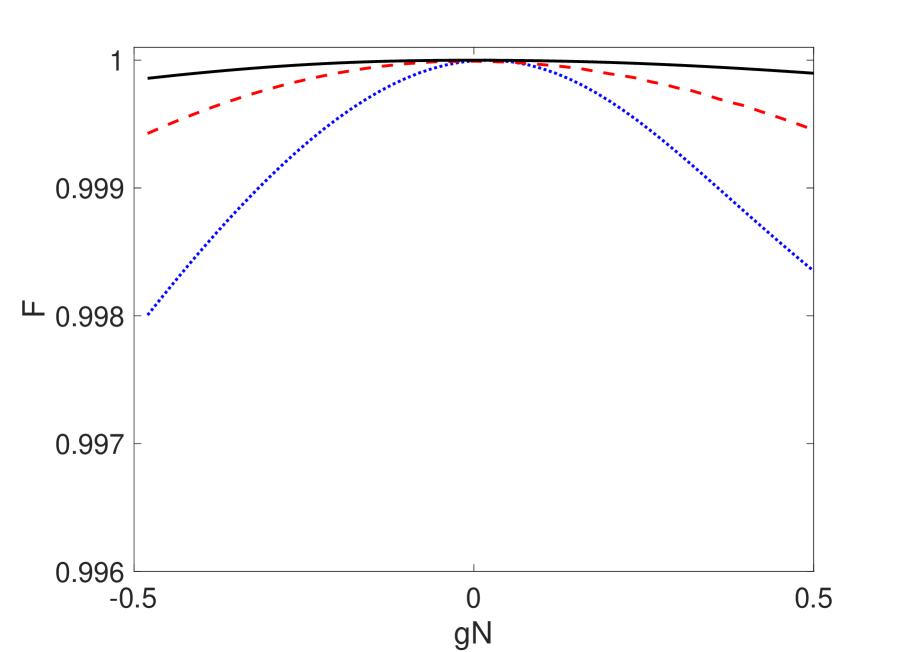
Figure 4: The dependence of the fidelity, defined as per Eq. (36) on nonlinearity strength $gN$, with the initial and final wave functions calculated by means of the imaginary-time evolution method. The state evolution, produced by different STA protocols, including inverse engineering (black solid), two-jump bang (blue dotted), and three-jump bang-bang (red dashed) schemes, is simulated with the help of the split-step method. Parameters are the same as those in Figs. 1 and 2.

Here we aim to explore stability of different STA protocols, designed on the basis of the inverse engineering, two-jump and three-jump bang-bang schemes, against the variation of the nonlinearity strength $gN$. To this end, we calculate the fidelity defined as

$$F=|\langle\tilde{\psi}_{f}(x)|\psi(x,t_{f})\rangle|^{2},$$ (36)

where wave function $|\tilde{\psi}_{f}\rangle$ is the final stationary state. Here the imaginary-time evolution method is used for obtaining the initial and final stationary states, and the state evolving along the shortcut trajectory is numerically calculated by means of the split-step method. As illustrated by Fig. 4, the smooth STA trajectory designed by dint of inverse engineering demonstrates, in general, better tolerance against the nonlinearity effects (which make the fidelity poorer), as two or three-jump protocols require abrupt changes of the frequency to satisfy the boundary conditions, which is a challenging condition. The STA protocols are more stable for $gN>0$ than for the opposite sign, as the Newtonian particle can easier escape from the effective potential well when the nonlinearity is self-attractive. As a matter of fact, the nonlinearity strongly affects the initial and final sizes of the BEC cloud (8). Under the action of weak nonlinearity, the difference between stationary states produced by the imaginary-time evolution method and the assumed Gaussian wave packets with initial and final values of $a$ [see Eq. ( 3)] is negligible. Furthermore, Fig. 5 shows the time evolution of the particle density, produced by the numerical solution of the time-dependent GP equation (1), and its counterpart predicted by the VA (dashed red curves). The figure corroborates the validity of the VA based on Gaussian ansatz (13), while the trap frequency changes abruptly at the switching points.

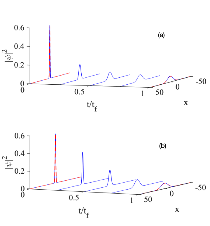
Figure 5: The evolution of the particle density (squared absolute value of the wave function) governed by the GP equation (1), with trap frequency $\omega(t)$ modulated in time by (a) the two-jump (17) and (b) the three-jump bang-bang (29) controls. Red dashed lines represent the initial and final particle densities calculated as per the variational approximation. They are virtually indistinguishable from the counterparts produced by the numerical solution of the GP equation. Parameters are the same as those in Fig. 2.

Apart from that, the implementation of our proposed protocols in realistic BEC experiments requires careful considerations. First, one has to apply two pinch coils to offset a purely magnetic Ioffe-Pritchard trap, thus producing an expulsive quadratic potential, instead of the HO one Khaykovich et al. (2002). An alternative way for achieving the same purpose is to combine a time-dependent red-detuned optical dipole trap with an additional blue-detuned antitrap Chen et al. (2010). Second, sudden changes of on-off controller entail the fast trap modulation, which might lead to unwanted intrinsic excitation of the state under the consideration Carr and Castin (2002). To avoid this, a multiple shooting method should be used for smoothing the bang-bang control scheme Yongcheng Ding . It is also important to mention that our idealized model amounts to an effectively 1D trap, produced by integrating the underlying three-dimensional GP equation in the transverse directions, under the action of the confinement in the transverse plane Salasnich et al. (2002). The use of magnetic and optical traps allows one to independently control of the axial and transverse frequencies. In fact, the radial-longitudinal coupling in the 3D setting sets a limit for the time scale on which the 1D equation is valid. It may be improved by increasing the waist of the trapping laser beam Torrontegui et al. (2012b). To be more precise, by taking into account longitudinal anharmonic perturbations, the lower validity bound for the ground-state decompression in the Gaussian trap is found to be $t_{f}\gg 3\hbar/8mw^{2}\omega_{f}^{2}$ Lu et al. (2014); Chen et al. (2010), with $m$ and $w$ being the mass of $\mbox{Rb}^{87}$ atoms and the laser-beam’s waist. Thus, after choosing the initial and finial frequencies, we obtain $t_{f}\gg 0.7$ for $w=50~{}\mathrm{\mu}$m and $t_{f}\gg 0.08$ for $w=150~{}\mathrm{\mu}$m, showing the validity of different STA protocols with high fidelity under realistic conditions.

IV.2 Excitation energy

The STA protocols support the frictionless cooling subject to the initial and final boundary conditions. However, the process itself is not adiabatic at all, thus excitation of the system on top of the stationary state may lead to detrimental effects. To address this issue, we define the time-average energy as

$$\bar{\mathcal{E}}=\frac{1}{t_{f}}\int_{0}^{t_{f}}\mathcal{E}(t)dt.$$ (37)

Substituting Eq. (6), and integrating once with the use of boundary conditions (8)-(10 ), we obtain

$$\bar{\mathcal{E}}=\frac{1}{t_{f}}\int_{0}^{t_{f}}\left(\dot{a}^{2}+\frac{1}{a^{2}}+\frac{3gN}{2\sqrt{2\pi}a}\right)dt.$$ (38)

The dependence of the so computed excitation energy on the nonlinearity strength is presented in Fig. 5. In principle, such an energy price of STA protocols is stipulated by the time-energy uncertainty, which implies increase of the (time-averaged) energy for shorter times. It is seen that the two-jump bang scheme produces smaller excitation energy, as the corresponding operation time is larger. With the same frequency bound, the operation time for the inverse-engineering scheme is larger than for the time-optimal bang-bang one, which leads to a smaller excitation energy as well. One can use another ansatz for the inverse engineering to minimize the excitation energy, as discussed in work Chen and Muga (2010). In addition, we point out that, as the bang and bang-bang schemes require sudden jumps to match the boundary conditions, the extra energy cost has to be paid at the edges, to fully implement these schemes.

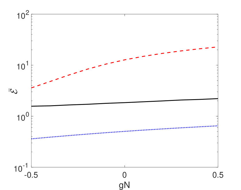
Figure 6: The dependence of time-average energy $\bar{\mathcal{E}}$, defined by Eq. (37), on the nonlinearity strength $gN$, for the inverse-engineering (black solid), two-jump bang (blue dotted), and three-jump bang-bang (red dashed) schemes. Parameters are the same as in Figs. 1 and 2.

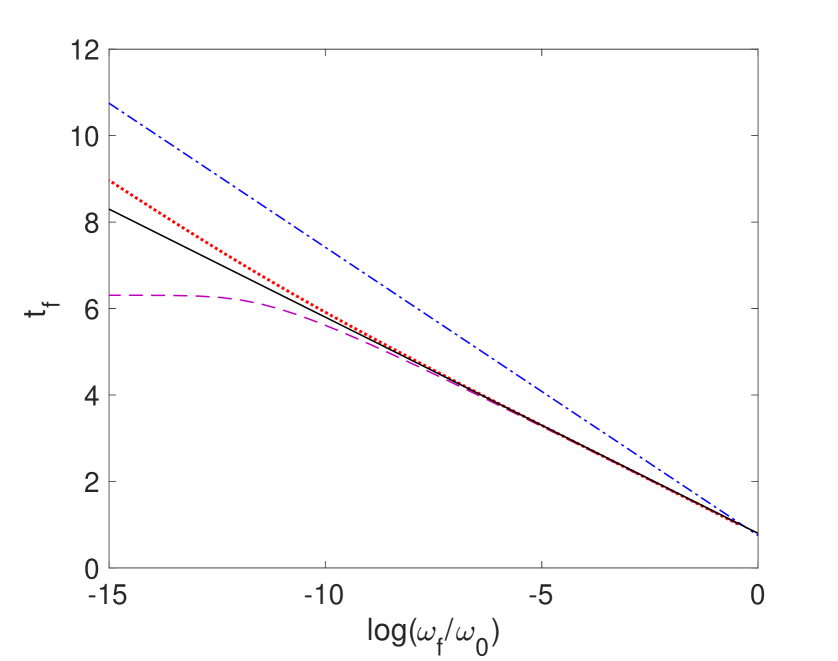
Figure 7: The minimum time for bang-bang scheme, as a function of $\log(\omega_{f}/\omega_{0})$: the TF limit (the dashed-dotted blue line), $gN=0$ (the solid black line), $gN=0.01$ (the dotted red line), and $gN=-0.01$ (the dashed purple line), other parameters being the same as in Fig. 2.

Finally, we note that the STA approach for atom cooling has fundamental implications for the third law of thermodynamics, with the atoms being the medium in a quantum refrigerator. Figure 7 quantifies the third law in this case, i.e., the minimal time diverges when the final trap frequency $\omega_{f}$, proportional to temperature, approaches zero. In a more general case, we see from Fig. 7 that the unattainability principle is quantified as

$$t_{f}\propto\log(a_{\mathrm{f}})+\frac{\pi}{4},$$ (39)

where $a_{\mathrm{f}}$ is a positive real solution of Eq. (12), and we keep the first two terms of its Taylor’s expansion around $gN=0$,

$$a_{\mathrm{f}}=\left(\frac{\omega_{0}}{\omega_{f}}\right)^{1/2}+\frac{gN}{4\sqrt{2\pi}}\left(\frac{\omega_{0}}{\omega_{f}}\right)^{3/2}+O^{2}(gN).$$ (40)

Interestingly, from Eq. (40) we recover the scaling law, $t_{f}\propto(\omega_{0}/\omega_{f})^{1/2}$, when $gN=0$, leading to the cooling rate, $R\propto T^{3/2}$, of the quantum refrigerator Salamon et al. (2009); Hoffmann et al. (2011); Chen and Muga (2010). In the TF limit, the second term in Eq. (40) becomes dominant, yielding $t_{f}\propto(\omega_{0}/\omega_{f})^{3/2}$, with the corresponding cooling rate $R\propto T^{2}$. Remarkably, the self-repulsive nonlinearity provides a larger exponent, therefore the repulsive interaction, acting in the course of the cooling process, may improve the cooling rate. When the nonlinear Feshbach heat engine Li et al. (2018) is considered, the attractive self-interaction implies the shorter time, leading to the improvement of the work. But in this case the stability is weaker, and the collapse of the wave packet exists at $\omega_{f}\ll 1$.

V Conclusion

To summarize, we have discussed the STA (shortcut to adiabaticity) for the expansion of weakly interacting BEC loaded in the HO (harmonic-oscillator) trap. The analysis is based on the use of the generalized Ermakov equation, derived from the VA (variational approximation) applied to the effective 1D Gorss-Pitaevskii equation. Exact solutions of the generalized Ermakov equation are inverse engineered to design smooth or piecewise-constant intermediate time dependences of the trap frequency, which realize the STA schemes. In particular, we focused on the minimal transition time and the minimization of the excitation energy produced by STA. To this end, the time-optimal solutions provided by the bang-bang scheme with a smooth polynomial ansatz, and by the two-jump bang scheme, have been compared. We conclude that the self-attractive nonlinearity in BEC can help to shorten the minimal time. The latter result which may have fundamental implications for the consideration of the quantum speed limit and third law of thermodynamics in quantum systems.

Finally, we point out several pending issues to be addressed. The stability with respect to the intrinsic BEC nonlinearity is reasonable, but the validity of the VA derivation of the Ermakov equation is predicated upon the accuracy of the Gaussian ansatz. Definitely, the bright soliton based on the hyperbolic-tangent function may be another option. Another noteworthy point is that the time-optimal solution has been obtained by means of the “bang-bang" scheme. It requires the sudden change of the trap frequency, that may be difficult to implement physically. One can further optimize the trajectory with more constraints imposed on the first, or even second, derivatives of the time dependence of the trap frequency. An alternative may be to use a smooth ansatz with polynomial and trigonometric functions for constructing the time-optimal “bang-bang" scheme, as discussed in Ref. Martikyan et al. (2020). All these results may apply to analyzing the transport, splitting, and compression of solitons Li et al. (2016, 2018), and also to various anharmonic potentials Xu et al. (2020); Lu et al. (2014), e.g. with quadratic terms.

Data Availability Statement

The data that support the findings of this study are available from the corresponding author upon reasonable request.

Appendix A

In the appendix, we first present an alternative way to derive the minimal time in TF limit for the consistence and further comparison. We use a set of equations for the density, $n$, and phase gradient, $\bigtriangledown\phi\left(x,t\right)$, of the wave function, represented in the Madelung form,

$$\psi\left(x,t\right)=\sqrt{n\left(x,t\right)}e^{i\phi\left(x,t\right)}.$$ (41)

Thus, the continuity equation derived from the GP equation (1 ) is

$$\frac{\partial n\left(x,t\right)}{\partial t}+\nabla\cdot\left(n\mathbf{\ v}\right)=0,$$ (42)

where the velocity of the superflow is defined by

$$\mathbf{v}=\frac{1}{2i}\frac{\left(\psi^{\ast}\nabla\psi-\psi\nabla\psi^{\ast}\right)}{|\psi|^{2}}\equiv\nabla\phi.$$ (43)

Next, we insert expression $(\ref{wave fun for n})$ in Eq. $(\ref{GP-equation})$, the real part of which yielding the Euler equation:

$$\frac{\partial\mathbf{v}}{\partial t}=-\bigtriangledown\left[-\frac{1}{2}\frac{\bigtriangledown^{2}\sqrt{n}}{\sqrt{n}}+\frac{\mathbf{v}^{2}}{2}+\frac{1}{2}\omega^{2}\left(t\right)x^{2}+gn\right].$$ (44)

In the case of the strongly self-repulsive condensate, the TF approximation Pitaevskii and Stringari (2003) allows one to omit the kinetic-energy term in Eq. $(\ref{Euler equation by hydro})$ (the first term of right-hand side), thus neglecting the quantum pressure, the result being

$$\frac{\partial\mathbf{v}}{\partial t}+\frac{\partial}{\partial x}\left(\frac{\mathbf{v}^{2}}{2}+\frac{1}{2}\omega^{2}\left(t\right)x^{2}+gn\right)=0$$ (45)

In the TF approximation, the initial equilibrium density distribution is $n_{0}(x,t)=(\mu-\omega^{2}(0)x^{2}/2)/g$, according to the time-independent GP equation with chemical potential $\mu$. The scaling approach to the hydrodynamic equation is commonly used to study dynamical properties of cold atomic system. It is based on ansatz of $n(x,t)=n_{0}[x/a(t)]/a(t)$, which satisfies the initial condition $n(x,0)=n_{0}(x)$ and $a(0)=1$. Then, one obtains the velocity field from the continuity equation $(\ref{continuity equation})$:

$$\mathbf{v}=\frac{\dot{a}\left(t\right)}{a\left(t\right)}x$$ (46)

Combining the TF limit and the scaling approach by inserting expression $(\ref{scaling of v})$ in Eq. $(\ref{Euler equation of TF})$ produces the evolution equation for scaling factor $a(t)$:

$$\ddot{a}+\omega^{2}\left(t\right)a=\frac{\omega_{0}^{2}}{a^{2}}.$$ (47)

Next, we need to transfer the initial ground state from trap frequency $\omega(0)=1$ at $t=0$ to the target state with $\omega(t_{f})=1/\gamma^{2}$. And the same boundary conditions, Eqs. (8-10), where $a_{\mathrm{i}}=1$ and $a_{\mathrm{f}}=\gamma^{4/3}$, are imposed to guarantee the realization of STA. Then, in terms of notation (20), the dynamical equations are rewritten as

$$\dot{x}_{1} = x_{2},$$ (48)

$$\dot{x}_{2} = -\tilde{u}x_{1}+\frac{1}{x_{1}^{2}},$$ (49)

where the control function $\tilde{u}(t)\equiv\omega^{2}(t)/\omega_{0}^{2}$ is used, subject to the bound $|\tilde{u}(t)|\leq\delta$, and variables $x_{1,2}$ satisfies obey the constraint

$$x_{2}^{2}+\tilde{u}x_{1}^{2}+\frac{2}{x_{1}}=c,$$ (50)

where $c$ is an integration constant. The time-optimal solution of the “bang-bang” type Stefanatos and Li (2012) for $\tilde{u}(t)$ is built as the same as $u(t)$ in (29). Applying the calculations similar to those presented in Eqs. $(\ref{first segment})$-$(\ref{tf for bangbang})$, the expressions for the duration of these two segments reads

$$t_{1}=\int_{a_{\mathrm{i}}}^{x_{1}^{B}}\frac{dx_{1}}{\sqrt{\delta x_{1}^{2}-2/x_{1}+c_{1}}},$$ (51)

$$t_{2}=\int_{x_{1}^{B}}^{a_{\mathrm{f}}}\frac{dx_{1}}{\sqrt{-\delta x_{1}^{2}-2/x_{1}+c_{2}}},$$ (52)

with $c_{1}=2/a_{\mathrm{i}}-\delta a_{\mathrm{i}}^{2}$ and $c_{2}=\delta a_{\mathrm{f}}^{2}+2/a_{\mathrm{f}}$. The intermediate switching point $x_{1}^{B}$ is found as

$$x_{1}^{B}=\sqrt{\frac{a_{\mathrm{f}}^{2}+a_{\mathrm{i}}^{2}}{2}+\frac{a_{\mathrm{i}}-a_{\mathrm{f}}}{\delta a_{\mathrm{i}}a_{\mathrm{f}}}}.$$ (53)

The minimum time in the TF limit, $t_{f}$, is now $t_{f}=t_{1}+t_{2}$.

Finally, we briefly present the time-optimal scheme for the ordinary Ermakov equation $(\ref{Ermakov equation})$. In this case, the boundary conditions, Eqs. (8-10), hold with $a_{\mathrm{i}}=1$ and $a_{\mathrm{f}}=1/\gamma$. Following Ref. Stefanatos et al. (2010), the minimal time $t_{f}=t_{1}+t_{2}$ is obtained, where the switching times $t_{1}$ and $t_{2}$ are

$$t_{1}=\frac{1}{\sqrt{\delta}}\sinh^{-1}\sqrt{\frac{(\gamma^{2}-1)(\gamma^{2}\delta-1)}{2\gamma^{2}(1+\delta)}},$$ (54)

$$t_{2}=\frac{1}{\sqrt{\delta}}\sin^{-1}\sqrt{\frac{(\gamma^{2}-1)(\gamma^{2}\delta+1)}{2(\gamma^{4}\delta-1)}}.$$ (55)

By setting $\delta=1$, we eventually obtain

$$t_{1} = -\frac{1}{r2}\log\left(\frac{\omega_{0}}{\omega_{f}}\right),$$ (56)

$$t_{2} = \pi/4,$$ (57)

as indicated in Fig. 7.

References

- Cohen-Tannoudji and Guéry-Odelin (2011) C. Cohen-Tannoudji and D. Guéry-Odelin, Advances in atomic physics: an overview (World Scientific, 2011).
- Kastberg et al. (1995) A. Kastberg, W. D. Phillips, S. L. Rolston, R. J. C. Spreeuw, and P. S. Jessen, Phys. Rev. Lett. 74, 1542 (1995).
- Anderson et al. (1994) D. Anderson, M. Lisak, B. Malomed, and M. Quiroga-Teixeiro, JOSA B 11, 2380 (1994).
- Couvert et al. (2008) A. Couvert, T. Kawalec, G. Reinaudi, and D. Guéry-Odelin, EPL (Europhysics Letters) 83, 13001 (2008).
- Bulatov et al. (1998) A. Bulatov, B. Vugmeister, A. Burin, and H. Rabitz, Phys. Rev. A 58, 1346 (1998).
- Bulatov et al. (1999) A. Bulatov, B. E. Vugmeister, and H. Rabitz, Phys. Rev. A 60, 4875 (1999).
- Salamon et al. (2009) P. Salamon, K. H. Hoffmann, Y. Rezek, and R. Kosloff, Physical Chemistry Chemical Physics 11, 1027 (2009).
- Henson et al. (2018) B. M. Henson, D. K. Shin, K. F. Thomas, J. A. Ross, M. R. Hush, S. S. Hodgman, and A. G. Truscott, Proceedings of the National Academy of Sciences 115, 13216 (2018).
- Torrontegui et al. (2013) E. Torrontegui, S. Ibánez, S. Martínez-Garaot, M. Modugno, A. del Campo, D. Guéry-Odelin, A. Ruschhaupt, X. Chen, and J. G. Muga, in Advances in atomic, molecular, and optical physics, Vol. 62 (Elsevier, 2013) pp. 117–169.
- Guéry-Odelin et al. (2019) D. Guéry-Odelin, A. Ruschhaupt, A. Kiely, E. Torrontegui, S. Martínez-Garaot, and J. G. Muga, Rev. Mod. Phys. 91, 045001 (2019).
- del Campo and Kim (2019) A. del Campo and K. Kim, New Journal of Physics 21, 050201 (2019).
- Muga et al. (2009) J. Muga, X. Chen, A. Ruschhaupt, and D. Guéry-Odelin, Journal of Physics B: Atomic, Molecular and Optical Physics 42, 241001 (2009).
- Chen et al. (2010) X. Chen, A. Ruschhaupt, S. Schmidt, A. del Campo, D. Guéry-Odelin, and J. G. Muga, Phys. Rev. Lett. 104, 063002 (2010).
- Schaff et al. (2010) J.-F. Schaff, X.-L. Song, P. Vignolo, and G. Labeyrie, Phys. Rev. A 82, 033430 (2010).
- Schaff et al. (2011a) J.-F. Schaff, X.-L. Song, P. Capuzzi, P. Vignolo, and G. Labeyrie, EPL (Europhysics Letters) 93, 23001 (2011a).
- Del Campo (2011) A. Del Campo, EPL (Europhysics Letters) 96, 60005 (2011).
- Schaff et al. (2011b) J.-F. Schaff, P. Capuzzi, G. Labeyrie, and P. Vignolo, New Journal of Physics 13, 113017 (2011b).
- Choi et al. (2011) S. Choi, R. Onofrio, and B. Sundaram, Phys. Rev. A 84, 051601 (2011).
- del Campo (2011) A. del Campo, Phys. Rev. A 84, 031606 (2011).
- Deffner et al. (2014) S. Deffner, C. Jarzynski, and A. del Campo, Phys. Rev. X 4, 021013 (2014).
- Papoular and Stringari (2015) D. J. Papoular and S. Stringari, Phys. Rev. Lett. 115, 025302 (2015).
- Deng et al. (2018) S. Deng, P. Diao, Q. Yu, A. del Campo, and H. Wu, Phys. Rev. A 97, 013628 (2018).
- Guéry-Odelin et al. (2014) D. Guéry-Odelin, J. G. Muga, M. J. Ruiz-Montero, and E. Trizac, Phys. Rev. Lett. 112, 180602 (2014).
- Rohringer et al. (2015) W. Rohringer, D. Fischer, F. Steiner, I. E. Mazets, J. Schmiedmayer, and M. Trupke, Scientific reports 5, 9820 (2015).
- Rezek et al. (2009) Y. Rezek, P. Salamon, K. H. Hoffmann, and R. Kosloff, EPL (Europhysics Letters) 85, 30008 (2009).
- Stefanatos et al. (2010) D. Stefanatos, J. Ruths, and J.-S. Li, Phys. Rev. A 82, 063422 (2010).
- Hoffmann et al. (2011) K. Hoffmann, P. Salamon, Y. Rezek, and R. Kosloff, EPL (Europhysics Letters) 96, 60015 (2011).
- Chen and Muga (2010) X. Chen and J. G. Muga, Phys. Rev. A 82, 053403 (2010).
- Li et al. (2011) Y. Li, L.-A. Wu, and Z. D. Wang, Phys. Rev. A 83, 043804 (2011).
- Stefanatos (2014) D. Stefanatos, Phys. Rev. A 90, 023811 (2014).
- Juliá-Díaz et al. (2012) B. Juliá-Díaz, E. Torrontegui, J. Martorell, J. G. Muga, and A. Polls, Phys. Rev. A 86, 063623 (2012).
- Yuste et al. (2013) A. Yuste, B. Juliá-Díaz, E. Torrontegui, J. Martorell, J. G. Muga, and A. Polls, Phys. Rev. A 88, 043647 (2013).
- Stefanatos and Paspalakis (2018) D. Stefanatos and E. Paspalakis, New Journal of Physics 20, 055009 (2018).
- Hatomura (2018) T. Hatomura, New Journal of Physics 20, 015010 (2018).
- Martínez et al. (2016) I. A. Martínez, A. Petrosyan, D. Guéry-Odelin, E. Trizac, and S. Ciliberto, Nature physics 12, 843 (2016).
- Faure et al. (2019) S. Faure, S. Ciliberto, E. Trizac, and D. Guéry-Odelin, American Journal of Physics 87, 125 (2019).
- Berry (2009) M. V. Berry, Journal of Physics A: Mathematical and Theoretical 42, 365303 (2009).
- del Campo (2013) A. del Campo, Phys. Rev. Lett. 111, 100502 (2013).
- Masuda and Nakamura (2008) S. Masuda and K. Nakamura, Phys. Rev. A 78, 062108 (2008).
- Torrontegui et al. (2012a) E. Torrontegui, S. Martínez-Garaot, A. Ruschhaupt, and J. G. Muga, Phys. Rev. A 86, 013601 (2012a).
- Chen et al. (2011) X. Chen, E. Torrontegui, and J. G. Muga, Phys. Rev. A 83, 062116 (2011).
- Castin and Dum (1996) Y. Castin and R. Dum, Phys. Rev. Lett. 77, 5315 (1996).
- Gritsev et al. (2010) V. Gritsev, P. Barmettler, and E. Demler, New journal of Physics 12, 113005 (2010).
- Ermakov (1880) V. P. Ermakov, Izv. Univ. Kiev (in Russian) 20, 1 (1880).
- Lewis (1967) H. R. Lewis, Phys. Rev. Lett. 18, 510 (1967).
- Reid and Ray (1980) J. L. Reid and J. R. Ray, Journal of Mathematical Physics 21, 1583 (1980).
- Ray (1980) J. R. Ray, Physics Letters A 78, 4 (1980).
- Rogers and Schief (2018) C. Rogers and W. K. Schief, Ermakov-type systems in nonlinear physics and continuum mechanics, In: N. Euler, editor, Nonlinear systems and their remarkable mathematical structures, (CRC Press, 2018) pp. 541–576.
- C. Rogers and Malomed (2020) W. S. C. Rogers and B. Malomed, Comm. Nonlin. Sci. Num. Sim. , 105091 (2020).
- Pitaevskii and Stringari (2003) L. P. Pitaevskii and S. Stringari, Bose–Einstein Condensation (Oxford University Press, Oxford, 2003).
- Pérez-García et al. (1996) V. M. Pérez-García, H. Michinel, J. I. Cirac, M. Lewenstein, and P. Zoller, Phys. Rev. Lett. 77, 5320 (1996).
- García-Ripoll et al. (1999) J. J. García-Ripoll, V. M. Pérez-García, and P. Torres, Phys. Rev. Lett. 83, 1715 (1999).
- Malomed (2002) B. A. Malomed, Progress in optics 43, 71 (2002).
- Li et al. (2016) J. Li, K. Sun, and X. Chen, Sci. Rep. 6, 38258 (2016).
- Li et al. (2018) J. Li, T. Fogarty, S. Campbell, X. Chen, and Th. Busch, New J. Phys. 20, 015005 (2018).
- Xu et al. (2020) T.-N. Xu, J. Li, T. Busch, X. Chen, and T. Fogarty, Phys. Rev. Research (2020).
- Stefanatos and Li (2012) D. Stefanatos and J.-S. Li, Phys. Rev. A 86, 063602 (2012).
- Salasnich et al. (2002) L. Salasnich, A. Parola, and L. Reatto, Phys. Rev. A 65, 043614 (2002).
- Quinn and Haque (2014) E. Quinn and M. Haque, Phys. Rev. A 90, 053609 (2014).
- Barak et al. (2008) A. Barak, O. Peleg, C. Stucchio, A. Soffer, and M. Segev, Phys. Rev. Lett. 100, 153901 (2008).
- Khaykovich et al. (2002) L. Khaykovich, F. Schreck, G. Ferrari, T. Bourdel, J. Cubizolles, L. D. Carr, Y. Castin, and C. Salomon, Science 296, 1290 (2002).
- Carr and Castin (2002) L. D. Carr and Y. Castin, Phys. Rev. A 66, 063602 (2002).
- (63) M. H. X. C. Yongcheng Ding, Tangyou Huang, arXiv:2002.11605 .
- Torrontegui et al. (2012b) E. Torrontegui, X. Chen, M. Modugno, A. Ruschhaupt, D. Guéry-Odelin, and J. G. Muga, Phys. Rev. A 85, 033605 (2012b).
- Lu et al. (2014) X.-J. Lu, X. Chen, J. Alonso, and J. G. Muga, Phys. Rev. A 89, 023627 (2014).
- Martikyan et al. (2020) V. Martikyan, D. Guéry-Odelin, and D. Sugny, Phys. Rev. A 101, 013423 (2020).