to be published in “Quantum Chemistry and Dynamics of Excited States: Methods and Applications”,
Eds. L. González and R. Lindh, 2020 Wiley-VCH

Excited-state calculations with quantum Monte Carlo

Abstract

Quantum Monte Carlo methods are first-principle approaches that approximately solve the Schrödinger equation stochastically. As compared to traditional quantum chemistry methods, they offer important advantages such as the ability to handle a large variety of many-body wave functions, the favorable scaling with the number of particles, and the intrinsic parallelism of the algorithms which are particularly suitable to modern massively parallel computers. In this chapter, we focus on the two quantum Monte Carlo approaches most widely used for electronic structure problems, namely, the variational and diffusion Monte Carlo methods. We give particular attention to the recent progress in the techniques for the optimization of the wave function, a challenging and important step to achieve accurate results in both the ground and the excited state. We conclude with an overview of the current status of excited-state calculations for molecular systems, demonstrating the potential of quantum Monte Carlo methods in this field of applications.

Chapter 0 Excited-state calculations with quantum Monte Carlo

1 Introduction

Quantum Monte Carlo (QMC) methods are a broad range of approaches which employ stochastic algorithms to simulate quantum systems, and have been used to study fermions and bosons at zero and finite temperature with very different many-body Hamiltonians and wave functions in the fields of molecular chemistry, condensed matter, and nuclear physics. While all QMC methods, despite the diversity of applications, share some core algorithms, we restrict ourselves here to the two zero-temperature continuum QMC methods that are most commonly used in electronic structure theory, namely, variational (VMC) and diffusion (DMC) Monte Carlo [1, 2, 3].

As compared to deterministic quantum chemistry approaches, solving the Schrödinger equation by stochastic means in VMC or DMC offers several advantages. The stochastic nature of the integration allows for a greater flexibility in the functional form of the many-body wave function employed, which can for instance include the explicit dependence on the inter-electronic distances. As a consequence, more compact wave functions can be used (the number of determinants needed to get the same energy is reduced by a few orders of magnitude) and, further, the dependence on the basis set is much weaker. Even though VMC and DMC are expensive, they have a favorable scaling with the system size (a mere polynomial $N^{4}$ in the number of electrons $N$), which has enabled simulations with hundreds and even thousands of electrons also in condensed matter, where traditional highly-correlated approaches are very difficult to apply. Finally, the intrinsically parallel nature of QMC algorithms renders these methods ideal candidates to take advantage of the massively parallel computers which are now available. An impressive example of such calculations is shown in Fig. 1 where the interaction energy dominated by dispersion is benchmarked with DMC for remarkably large complexes [4].

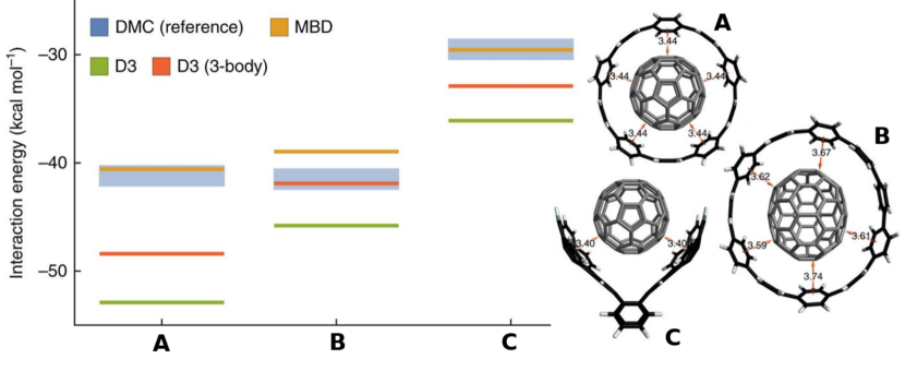
Figure 1: Interaction energies of the complexes A–C computed with DMC and density functional theory with two different dispersion corrections (D3) and the many-body dispersion method (MBD). Adapted from Ref. [4].

That said, when inspecting the literature, it is evident that VMC and DMC methods have traditionally been employed to calculate mainly total energies and total energy differences as the computation of quantities other than the energy is more complicated. QMC calculations are for instance generally carried out on geometries obtained at a different level of theory and also the construction of the many-body wave function and its optimization are not straightforward. Particular care must in fact be paid to this step since the residual DMC error can be larger than sometimes assumed in the past, when calculations were anyhow limited to relatively simple wave functions and it was not feasible to extensively explore the dependence of the results on the choice of wave function. We will come back below to this point, which is especially relevant for excited states.

The last few years have however seen remarkable progress in methodological developments to overcome these and other limitations, as well as extend the applicability of QMC to larger systems both in the ground and the excited state. In particular, robust optimization algorithms for the parameters in the wave function have been developed for ground states [5, 6, 7, 8] and extended to the state-average [9] as well as state-specific [10, 11] optimization of excited states. Importantly, it has recently become possible to efficiently compute the quantities needed in these optimization schemes (i.e. the derivatives of the wave function and the action of the Hamiltonian on these derivatives) at a cost per Monte Carlo step which scales like the computation of the energy alone [12, 13, 14]. Consequently, the determinantal component of a QMC wave function does not have to be borrowed from other quantum chemical calculations but can be consistently optimized within VMC after the addition of the correlation terms depending on the inter-electronic distances. These developments also enable the concomitant optimization of the structural parameters in VMC even when large determinantal expansions are employed in the wave function [14, 15]. The possibility of performing molecular dynamics simulations with VMC forces has also been recently demonstrated [16, 17].

Researchers have also been actively investigating more complex functional forms  [18, 19, 20, 21, 22] to recover missing correlation and allow a more compact wave function than the one obtained with a multi-determinant component. A local correlation description has also been shown to be a promising route to achieve smaller expansions and reduced computational costs for ground and excited states [23, 24]. In parallel, algorithms have been explored for a more automatic selection of the determinantal component, avoiding the possible pitfalls of a manual choice based on chemical intuition [25, 26, 27, 28, 15, 29, 30]. Importantly, effort has been devoted to develop algorithms for the computation of quantities other than the energy via estimators characterized by reduced fluctuations as well as wave function bias [31, 32, 33, 5, 34, 35, 36]. In addition to these methodological advances, various tools have become available to facilitate the calculations, such as tables of pseudopotentials and corresponding basis sets especially constructed for QMC [37, 38, 39, 40, 41, 42]. Finally, multi-scale methods have been proposed to include the effects of a (responsive) environment on an embedded system treated with QMC [43, 44, 45, 46, 47, 48].

After a brief description of the VMC and DMC methods, we will focus here on some of these recent developments, giving special attention to the algorithms employed to optimize the variational parameters in the wave function. We will then review relevant work and recent advances in the calculation of excited states and their properties, mainly for molecular systems. We note that useful sources for QMC are the introductory book to Monte Carlo methods and their use in quantum chemistry [49], and the reviews on QMC methods and their applications to solids [1, 50, 51, 52] and to noncovalent interactions [53]. A detailed introduction to VMC and DMC can be found in Ref. [54]. Finite-temperature path integral Monte Carlo methods are covered in Ref. [55].

2 Variational Monte Carlo

Variational Monte Carlo is the simplest flavor of QMC methods and represents a generalization of classical Monte Carlo to compute the multidimensional integrals in the expectation values of quantum mechanical operators. The approach enables the use of any “computable” wave function without severe restrictions on its functional form. This must be contrasted to other traditional quantum chemical methods which express the wave function as products of single particle orbitals in order to perform the relevant integrals analytically.

To illustrate how to compute an expectation value stochastically, let us consider the variational energy $E_{\mathrm{v}}$, namely, the expectation value of the Hamiltonian $\hat{H}$ on a given wave function $\Psi$, which we rewrite as

$$E_{\mathrm{v}}=\frac{\int\Psi(\mathbf{R})^{*}\hat{H}\Psi(\mathbf{R})\mathrm{d}\mathbf{R}}{\int|\Psi(\mathbf{R})|^{2}\mathrm{d}\mathbf{R}}=\frac{\int|\Psi(\mathbf{R})|^{2}\frac{\hat{H}\Psi(\mathbf{R})}{\Psi(\mathbf{R})}\mathrm{d}\mathbf{R}}{\int|\Psi(\mathbf{R})|^{2}\mathrm{d}\mathbf{R}}=\int\rho(\mathbf{R})E_{\mathrm{L}}(\mathbf{R})\mathrm{d}\mathbf{R}\,,$$ (1)

where we have introduced the probability distribution, $\rho(\mathbf{R})$, and the local energy, $E_{\mathrm{L}}(\mathbf{R})$, defined as

$$\rho(\mathbf{R})=\frac{|\Psi(\mathbf{R})|^{2}}{\int|\Psi(\mathbf{R})|^{2}\mathrm{d}\mathbf{R}}\ \ \ \text{and}\ \ \ E_{\mathrm{L}}(\mathbf{R})=\frac{\hat{H}\Psi(\mathbf{R})}{\Psi(\mathbf{R})}\,,$$ (2)

with $\mathbf{R}$ denoting the $3N$ coordinates of the electrons. We note that we can interpret $\rho(\mathbf{R})$ as a probability distribution since it is always non-negative and integrates to one.

The integral can then be estimated by averaging the local energy computed on a set of $M$ configurations $\{\mathbf{R}_{k}\}$ sampled from the probability density $\rho(\mathbf{R})$ as

$$E_{\mathrm{v}}\approx\bar{E}_{\mathrm{L}}=\frac{1}{M}\sum_{k}^{M}E_{\mathrm{L}}(\mathbf{R}_{k})\,.$$ (3)

According to the central limit theorem, this estimator converges to the exact value, $E_{\mathrm{v}}$, with increasing number of Monte Carlo configurations with a statistical uncertainty which decreases as

$$\text{err}(\bar{E}_{\mathrm{L}})\propto\frac{\sigma_{\mathrm{v}}}{\sqrt{M}}\,,$$ (4)

where $\sigma_{\mathrm{v}}^{2}=\int\rho(\mathbf{R})(E_{\mathrm{L}}(\mathbf{R})-E_{\mathrm{v}})^{2}\mathrm{d}\mathbf{R}$ is the variance of the local energy. For this relation to hold, the chosen wave function must yield a finite variance of the sampled quantity, in this case, the local energy. A typical VMC run is illustrated in Fig. 2, where the local energy is computed at each Monte Carlo step together with its running average.

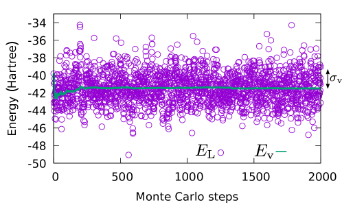
Figure 2: Local energy (circle) and its running average (green line) in a typical VMC run. The size of the root-mean-square fluctuations of the local energy, $\sigma_{\mathrm{v}}$, is also indicated.

Importantly, the statistical uncertainty decreases as $1/\sqrt{M}$ independently of the number of dimensions in the problem so that Monte Carlo displays a faster convergence than deterministic numerical integration already for small numbers of dimensions. Furthermore, as the trial wave function improves, the Monte Carlo estimate of the variational energy requires fewer Monte Carlo steps to converge. In the limit of the wave function being an exact eigenstate of the Hamiltonian, the variance approaches zero and a single configuration is sufficient to obtain the exact variational energy. This zero-variance principle applies straightforwardly to the Hamiltonian and operators commuting with the Hamiltonian (therefore, the large number of total energy calculations found in the QMC literature). This principle can however be generalized to arbitrary observables by formulating an equivalent, improved estimator having the same average but a different, reduced variance [31]. Reduced variance estimators have been derived for the computation of electron density [56, 57], the electron pair densities [34], interatomic forces [33, 35], and other derivatives of the total energy [5].

In practice, the probability distribution $\rho(\mathbf{R})$ is sampled with the Metropolis-Hastings algorithm by simulating a Markov chain. This is a sequence of successive configurations, ${\mathbf{R}}_{1},\ldots,{\mathbf{R}}_{M}$, generated with a transition probability, $P(\mathbf{R}^{\prime}|\mathbf{R})$, where the transition to a new configuration $\mathbf{R}^{\prime}$ only depends on the current point $\mathbf{R}$. The transition probability is stochastic, which means that it has the following properties:

$$P(\mathbf{R}^{\prime}|\mathbf{R})\geq 0\ \ \ \text{and}\ \ \ \int P(\mathbf{R}^{\prime}|\mathbf{R})\mathrm{d}\mathbf{R}^{\prime}=1\,.$$ (5)

Repeated application of $P$ generates a Markov chain which converges to the target distribution $\rho$ as

$$\lim\limits_{M\rightarrow\infty}\int P(\mathbf{R}|\mathbf{R}_{M})\ldots P(\mathbf{R}_{2}|\mathbf{R}_{1})\rho_{\mathrm{init}}(\mathbf{R}_{1})\mathrm{d}\mathbf{R}_{1}\ldots\mathbf{R}_{M}=\rho(\mathbf{R})\,,$$ (6)

if $P$ is ergodic (it possible to move between two different configurations in a finite number of steps) and fulfills the so-called stationarity condition:

$$\int P(\mathbf{R}^{\prime}|\mathbf{R})\rho(\mathbf{R})\mathrm{d}\mathbf{R}=\rho(\mathbf{R}^{\prime})\,.$$ (7)

The stationarity condition tells us that, if we start from the desired distribution $\rho$, we will continue to sample $\rho$. Moreover, if the stochastic probability $P$ is ergodic, it is possible to show that this condition ensures that any initial distribution will evolve to $\rho$ under repeated applications of $P$.

In the Metropolis-Hastings algorithm, the transition to a new state is carried out in two steps: a new configuration is generated by a (stochastic) proposal probability and the proposed step is then accepted or rejected with an acceptance probability. The latter can be constructed so that the combined proposal and acceptance steps fulfill the stationarity condition. Most importantly, the acceptance depends only on ratios of $\rho(\mathbf{R})$ so that the generally unknown normalization of the distribution $\rho$ is not required. We note that it is desirable to reduce sequential correlation among configurations. Proposing large steps to quickly explore the phase space must therefore be balanced against the rate of acceptance which decreases with large steps. For these reasons, electrons are generally moved one at the time to allow larger steps with a reasonable acceptance rate, a necessary feature as the system size grows since the size of the move would need to be decreased to have a reasonable acceptance of a move of all particles.

VMC is a very powerful method as the stochastic nature of integration gives a lot of freedom in the choice of the functional form of the wave function. It also allows us to learn a great deal about a system by exploring which ingredients in the wave function are necessary for its accurate description. Finally, in VMC, there is no sign problem associated with Fermi statistics, which generally plagues other quantum Monte Carlo approaches as we will see below. The obvious drawback is that, for each particular problem, a parametrization of the wave function has to be constructed. This process can be non-trivial and tends to be biased towards simpler electronic states: for example, it is easier to construct a good wave function for a closed-shell than an open-shell system so that the energy of the former will be closer to the exact result than for the latter. Furthermore, properties other than the energy (or expectation values of operators commuting with the Hamiltonian) can be significantly less accurate since they are first order in the error of the wave function instead of second order as for the energy. It has however been shown that it is possible to extend this favorable property of the energy to arbitrary observables by using modified estimators which lead not only to reduced fluctuations but also to a reduced bias due to the wave function [33] as convincingly demonstrated in some promising applications [34, 36, 57, 33]. An example of this so-called zero-variance (ZV) zero-bias (ZB) approach applied to the computation of the intracule density is shown in Fig. 3: the use of a ZV estimator significantly reduces the statistical fluctuations of the density and the further ZB formulation yields the correct result even when a simple Hartree-Fock wave function is employed. In general, the VMC approach is an extremely valuable tool and, in recent years, its use and impact has in fact become greater thanks to the availability of robust methods to optimize the many parameters in the wave function and, consequently, to increase the accuracy of the observables of interest already at the VMC level. Finally, characterizing and optimizing the trial wave function in VMC represents a necessary ingredient for more advanced projector Monte Carlo methods like the diffusion Monte Carlo approach described in next Section.

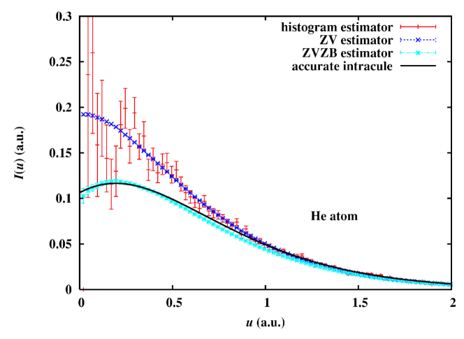
Figure 3: Spherically-averaged intracule density $I(u)$ as a function of the electron-electron distance $u$ for the He atom calculated in VMC with a histogram, a zero-variance, and a zero-variance zero-bias estimator and the same Hartree-Fock wave function (without a Jastrow factor). Adapted from Ref. [34].

3 Diffusion Monte Carlo

Projector Monte Carlo methods are QMC approaches which remove (at least in part) the bias of the trial wave function which characterizes VMC calculations. They are a stochastic implementation of the power method for finding the dominant eigenstate of a matrix or integral kernel. In a projector Monte Carlo method, one uses an operator that inverts the spectrum of $\hat{H}$ to project out the ground state of $\hat{H}$ from a given trial state.

Diffusion Monte Carlo (DMC) uses the exponential projection operator $e^{-t(\hat{H}-E_{\mathrm{T}})}$ with $E_{\mathrm{T}}$ a trial energy whose role will become immediately apparent. To understand the effect of applying this operator on a given wave function, let us consider a trial wave function $\Psi$, which we expand on the eigenstates of $\hat{H}$, $\Psi_{i}$ with eigenvalues $E_{i}$. In the limit of infinite time $t$, we then obtain

$$\lim\limits_{t\rightarrow\infty}e^{-t(\hat{H}-E_{\mathrm{T}})}|\Psi\rangle=\lim\limits_{t\rightarrow\infty}\sum_{i}e^{-t(E_{i}-E_{\mathrm{T}})}|\Psi_{i}\rangle\langle\Psi_{i}|\Psi\rangle=\lim\limits_{t\rightarrow\infty}e^{-t(E_{0}-E_{\mathrm{T}})}|\Psi_{0}\rangle\langle\Psi_{0}|\Psi\rangle\,,$$ (8)

where, in the last equality, we used that the coefficients in front of the higher eigenstates decay exponentially faster than the one of the ground state. If we adjust $E_{T}$ to $E_{0}$, the projection will yield the ground state $\Psi_{0}$. Note that the starting wave function must have a non-zero overlap with the ground-state one.

In the position representation, this projection can be rewritten as

$$\Psi(\mathbf{R}^{\prime},t)=\int G(\mathbf{R}^{\prime}|\mathbf{R},t)\Psi(\mathbf{R})\mathrm{d}\mathbf{R}\,,$$ (9)

where we introduced the coordinate Green’s function defined as

$$G(\mathbf{R}^{\prime}|\mathbf{R},t)=\langle\mathbf{R}^{\prime}|{e^{-t(\hat{H}-E_{\mathrm{T}})}}|{\mathbf{R}}\rangle\,.$$ (10)

This representation readily allows us to see how to translate the projection into a Markov process provided that we can sample the Green’s function and the trial wave function. For fermions, the wave function is antisymmetric and cannot therefore be interpreted as a probability distribution, a fact that we will ignore for the moment.

A further complication is that the exact form of the Green’s function is not known. Fortunately, in the limit of small-time steps $\tau$, Trotter’s theorem tells us that we are allowed to consider the potential and kinetic energy contributions separately since

$$e^{-\tau(\hat{T}+\hat{V})}=e^{-\tau\hat{T}}e^{-\tau\hat{V}}+{\cal O}(\tau^{2})\,,$$ (11)

so that

$$\langle\mathbf{R}^{\prime}|e^{-\tau\hat{H}}|\mathbf{R}\rangle \approx \langle\mathbf{R}^{\prime}|e^{-\tau\hat{T}}e^{-\tau\hat{V}}|\mathbf{R}\rangle=\int\mathrm{d}\mathbf{R}^{\prime\prime}\langle\mathbf{R}^{\prime}|e^{-\tau\hat{T}}|\mathbf{R}^{\prime\prime}\rangle\langle\mathbf{R}^{\prime\prime}|e^{-\tau\hat{V}}|\mathbf{R}\rangle$$ (12)

$$= \langle\mathbf{R}^{\prime}|e^{-\tau\hat{T}}|\mathbf{R}\rangle e^{-\tau{V}(\mathbf{R})}\,.$$

Therefore, we can rewrite the Green’s function in the short-time approximation as

$$G(\mathbf{R}^{\prime}|\mathbf{R},\tau)=(2\pi\tau)^{-3N/2}\,\exp\left[-\frac{(\mathbf{R}^{\prime}-\mathbf{R})^{2}}{2\tau}\right]\,\exp\left[-\tau\,({V}(\mathbf{R})-E_{\mathrm{T}})\right]+{\cal O}(\tau^{2})\,,$$ (13)

where the first (stochastic) factor is the Green’s function for diffusion while the second term multiplies the distribution by a positive scalar. The repeated application of the short-time Green’s function to obtain the distribution at longer times (Eq. 9) can be interpreted as a Markov process with the difference that the Green’s function is not normalized due to the potential term, and we therefore obtain a weighted random walk.

The basic DMC algorithm is rather simple:

1. An initial set of $M_{0}$ so-called walkers $\mathbf{R}_{1},\ldots,\mathbf{R}_{M_{0}}$ is generated by sampling the trial wave function $\Psi(\mathbf{R})$ with the Metropolis algorithm as in VMC. This is the zero-th generation and the number of configurations is the population of the zero-th generation.

2. Each walker diffuses as $\mathbf{R}^{\prime}=\mathbf{R}+\xi$ where $\xi$ is sampled from the 3$N$-dimensional Gaussian distribution $g(\xi)=(2\pi\tau)^{-3N/2}\exp\left(-\xi^{2}/2\tau\right)$.

3. For each walker, we compute the factor

   $$p=\exp\left[-\tau({V}(\mathbf{R})-E_{\mathrm{T}})\right]\,.$$ (14)

   and perform the so-called branching step, namely, we branch the walker by treating $p$ as the probability to survive at the next step: if $p<1$, the walker survives with probability $p$ while, if $p>1$, the walker continues and new walkers with the same coordinates are created with probability $p-1$. This is achieved by creating a number of copies of the current walker equal to the integer part of $p+\eta$ where $\eta$ is a random number between (0,1). The branching step causes walkers to live in regions with a low potential ${V}<E_{\mathrm{T}}$ and die in regions with high $V$.

4. We adjust $E_{\mathrm{T}}$ so that the overall population fluctuates around the target value $M_{0}$.

Steps 2-4 are repeated until a stationary distribution is obtained and the desired properties are converged within a given statistical accuracy. A schematic representation of the evolution for a simple one-dimensional problem is shown in Fig. 4. Since the short-time expression of the Green’s function is only valid in the limit of $\tau$ approaching zero, in practice, DMC calculations must be performed for different values of $\tau$ and the results extrapolated for $\tau$ which goes to zero.

Figure 4: Schematic representation of a DMC simulation showing the evolution of the walkers in a one-dimensional potential $V(x)$. The walkers are uniformly distributed at the start and converge to the ground-state distribution $\Psi_{0}$ after a number of time steps (adapted from Ref. [1]).

The direct sampling of this Green’s function proves however to be highly inefficient and unstable since the potential can vary significantly from configuration to configuration or also be unbounded like the Coulomb potential. For example, the electron-nucleus potential diverges to minus infinity as the two particles approach each other, and the branching factor will give rise to an unlimited number of walkers. Even if the potential is bounded, the approach becomes inefficient with increasing size of the system since the branching factor also grows with the number of particles. These difficulties can be overcome by using importance sampling, where the trial wave function, $\Psi$, is used to guide the random walk. Starting from Eq. 9, we multiply each side by $\Psi(\mathbf{R}^{\prime})$ and define the probability distribution $f(\mathbf{R},t)=\Psi(\mathbf{R},t)\Psi(\mathbf{R})$ which satisfies

$$f(\mathbf{R}^{\prime},t)=\int\tilde{G}(\mathbf{R}^{\prime}|\mathbf{R},t)\Psi(\mathbf{R})^{2}\mathrm{d}\mathbf{R}\,,$$ (15)

where the importance sampled Green’s function is given by

$$\tilde{G}(\mathbf{R}^{\prime}|\mathbf{R},t)=\Psi(\mathbf{R}^{\prime})\langle{\mathbf{R}}^{\prime}|{e^{-t(\hat{H}-E_{\mathrm{T}})}}|{\mathbf{R}}\rangle/\Psi({\mathbf{R}})\,.$$ (16)

In the limit of long times, this distribution $f(\mathbf{R},t)$ approaches $\Psi_{0}(\mathbf{R})\Psi(\mathbf{R})$.

Assuming for the moment that $\Psi(\mathbf{R}^{\prime})/\Psi(\mathbf{R})>0$, the importance sampled Green’s function in the short-time approximation becomes

$$\tilde{G}(\mathbf{R}^{\prime}|\mathbf{R},\tau)\approx(2\pi\tau)^{-\frac{3}{2}N}\exp\left[-\frac{(\mathbf{R}^{\prime}-\mathbf{R}-\tau\mathbf{V}(\mathbf{R}))^{2}}{2\tau}\right]\exp\left[-\tau(E_{\mathrm{L}}(\mathbf{R})-E_{\mathrm{T}})\right]\,,$$ (17)

where one has assumed that the drift-velocity $\mathbf{V}(\mathbf{R})=\nabla\Psi(\mathbf{R})/\Psi(\mathbf{R})$ and the local energy (Eq. 2) are constant in the step from $\mathbf{R}$ to $\mathbf{R}^{\prime}$. There are two important new features of $\tilde{G}$. First, the quantum velocity $\mathbf{V}(\mathbf{R})$ pushes the walkers to regions where $\Psi(\mathbf{R})$ is large. In addition, the local energy $E_{\mathrm{L}}$ instead of the potential appears in the branching factor. Since the local energy becomes constant and equal to the eigenvalue as the trial wave function approaches the exact eigenstate, we expect that, for a good trial wave function, the fluctuations in the branching factor will be significantly smaller. In particular, imposing the cusp conditions on the wave function will remove the instabilities coming from the singular Coulomb potential. The simple DMC algorithm can be easily modified by sampling the square of the trial wave function in a VMC calculation (step 1), drifting before diffusing the walkers (step 2), and employing the exponential of the local energy as branching factor (step 3). Several important modifications to this bare-bone algorithm can and should be introduced to reduce the time-step error, which are described in detail along with further improvements in Ref. [58].

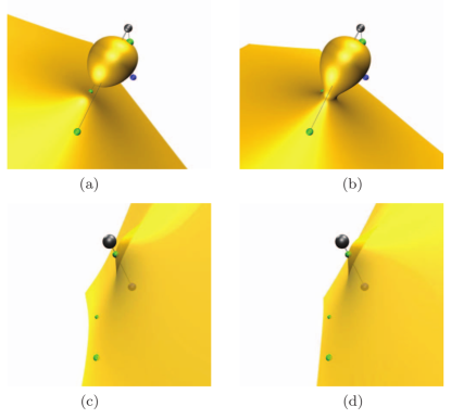
Figure 5: A 3-dimensional slice of the nodal surface of the N (top) and P (bottom) atoms obtained as a scan of the wave function moving one electron and keeping the others at snapshot positions (green/blue spheres). The black spheres mark the positions of the nucleus. (a, c) Nearly exact nodes and (b, d) Hartree-Fock nodes. Adapted from Ref. [59].

Up to this point, we have assumed that the wave function does not change sign. This is true for the ground state of a bosonic system, whose wave function can be in principle projected exactly in a DMC simulation. For fermions, however, a move of a walker can lead to a change of sign due to the antisymmetry of the wave function. While it is possible to work with weights that carry a sign, the stochastic realization of such a straightforward approach is not stable since the separate evolution of the populations of positive and negative walkers will lead to the same bosonic solution, and the fermionic signal will be exponentially lost in the noise. This is known as the fermionic sign problem. To circumvent this problem, we can simply forbid moves in which the sign of the trial wave function changes and the walker crosses the nodes which are defined as (3N$-$1)-dimensional surface where the trial wave function is zero. Imposing the nodal constraint can be achieved either by deleting the walkers which attempt to cross the nodes or by using the short-time importance sampled Green’s function, where walkers do not cross the nodes in the limit of zero time step. This procedure is known as the fixed-node approximation. Forbidding node crossing is equivalent to finding the exact solution with the boundary condition of having the same nodes as the trial wave function. The Schrödinger equation is therefore solved exactly inside the nodal regions but not at the nodes where the solution will have a discontinuity of the derivatives. The fixed-node solution will be exact only if the nodes of the trial wave function are exact. In general, the fixed-node energy will be an upper bound to the exact energy. A cut through the nodal surface of the N and P atoms for a simple Hartree-Fock and a highly-accurate wave function (Fig. 5) reveals that considerable differences are possible which are atom dependent and directly translate in a larger size of the fixed-node error for the N atom when a mono-determinantal wave function is used [59].

The fixed-node DMC algorithm can be also used to study excited states. There is no particular difficulty in applying DMC to the lowest state of a given symmetry by simply employing a trial wave function of the proper spatial and spin symmetry. For excited states which are energetically not the lowest in their symmetry, all that we know is that fixed-node DMC will give the exact solution if we employ a trial wave function with the exact nodes [60]. However, there is no variational principle and one may expect a stronger dependence of the result on the choice of the wave function, which is now not only used to overcome the fermion-sign problem but also to select the state of interest. In our experience, unless we intentionally generate a wave function with a large overlap with the ground-state one, we do not suffer from lack of variationality in the excited-state calculation. In fact, the use of simplistic wave functions (e.g. HOMO-LUMO Hartree-Fock, configuration-interaction singles, non-reoptimized truncated complete-active-space expansions) has been shown to generally lead to an overestimation of the excitation energy also in DMC, especially when the excited state has a strong multi-determinant character [61]. Consequently, while DMC cannot cure the shortcomings of a poor wave function, such a choice will likely yield smaller fixed-node errors in the ground than the excited state and, ultimately, an overestimation of the DMC excitation energy.

4 Wave functions and their optimization

The key quantity which determines the quality of a VMC and a fixed-node DMC calculation is the trial wave function. The choice of the functional form of the wave function and its optimization within VMC are key steps in a QMC calculation as they are crucial elements to obtain accurate results already at the VMC level and to reduce the fermionic-sign error in a subsequent DMC calculation.

Most QMC studies of electronic systems have employed trial wave functions of the so-called Jastrow-Slater form, that is, the product of a sum of determinants of single-particle orbitals and a Jastrow correlation factor as

$$\Psi=\mathcal{J}\sum_{k}c_{k}D_{k}\,,$$ (18)

where $D_{k}$ are Slater determinants of single-particle orbitals and the Jastrow correlation function is a positive function of the interparticle distances, which explicitly depends on the electron-electron separations. The Jastrow factor plays an important role as it is used to impose the Kato cusp conditions and to cancel the divergences in the potential at the inter-particle coalescence points. This leads to a smoother behavior of the local energy and therefore more accurate and efficient VMC as well as DMC calculations thanks to the smaller time-step errors and reduced fluctuations in the branching factor.

Moreover, the Jastrow factor introduces important correlations beyond the short electron-electron distances [62] and QMC wave functions enjoy therefore a more compact determinantal expansion than conventional quantum chemical methods. Even though the positive Jastrow function does not directly alter the nodal structure of the wave function which is solely determined by the antisymmetric part, the optimal determinantal component in a QMC wave function will be different than the one obtained for instance in a multi-configuration self-consistent-field calculation (MCSCF) in the absence of the Jastrow factor. Upon optimization of the QMC wave function, the determinantal component will change and it is often possible to obtain converged energy differences in VMC and DMC with relatively short determinantal expansions in a chosen active space. Furthermore, thanks to the presence of the Jastrow factor, QMC results are generally less dependent on the basis set. For instance, excitations and excited-state gradients show a faster convergence with basis set than multiconfigurational approaches, and an augmented double basis set with polarization functions is often sufficient in both VMC and DMC for the description of excited-state properties [63, 24, 64].

Important requirement for the optimization of the many parameters in a QMC wave function is the ability to efficiently evaluate the derivatives of the wave function and the action of the Hamiltonian on these derivatives during a QMC run. In general, this is central to the computation of low-variance estimators of derivatives of the total energy as, for instance, the derivatives with respect to the nuclear coordinates (i.e. interatomic forces). Computing these derivatives at low cost is therefore crucial to enable higher accuracy as well as to extend the application of QMC to larger systems and a broader range of molecular properties. Automatic differentiation was successfully applied for the computation of analytical derivatives [12] but the application to large computer codes is not straightforward and the memory requirements might become prohibitive.

Recently, an efficient and simple analytical formulation has been developed to compute a complete set of derivatives of the wave function and of the local energy with the same scaling per Monte Carlo step as computing the energy alone both for single- and multi-determinant wave functions [13, 14]. This formulation relies on the straightforward manipulation of matrices evaluated on the occupied and virtual orbitals and can be very simply illustrated in the case of a single determinant in the absence of a Jastrow factor:

$$D=\det(A)=|\phi_{1}\phi_{2}\ldots\phi_{N}|\,,$$ (19)

where $A$ is a Slater matrix defined in terms of the $N$ occupied orbitals, $\phi_{i}$, as $A_{ij}=\phi_{j}(\mathbf{r}_{i})$. For this wave function, it is not difficult to show that the action of a one-body operator $\hat{O}=O(\mathbf{r}_{1})+\ldots+O(\mathbf{r}_{N})$ on the determinant can be written as the trace between the inverse $A$ matrix and an appropriate matrix $B$,

$$\frac{\hat{O}D}{D}=\operatorname{tr}(A^{-1}B)\,,$$ (20)

where $B$ is obtained by applying the operator $O(\mathbf{r})$ to the elements of $A$ as

$$B_{ij}=(O\phi)_{j}(\mathbf{r}_{i})\,.$$ (21)

For instance, if we consider the kinetic operator, we obtain

$$\hat{T}\det(A)=-\frac{1}{2}\sum_{i}\Delta_{i}\det(A)=-\frac{1}{2}\sum_{i}\;\left[\sum_{j}\Delta\phi_{j}({\mathbf{r}}_{i})\,(A^{-1})_{ji}\det(A)\right]\,,$$ (22)

which can be rewritten as

$$\frac{\hat{T}\det(A)}{\det(A)}=\sum_{i}\sum_{j}B_{ij}^{\mathrm{kin}}\,(A^{-1})_{ji}=\operatorname{tr}(A^{-1}B^{\mathrm{kin}})\,,$$ (23)

where $B^{\mathrm{kin}}_{ij}=-\frac{1}{2}\Delta_{i}A_{ij}=-\frac{1}{2}\Delta\phi_{j}({\mathbf{r}}_{i})$. It is possible to show that an equivalent trace expression holds also in the presence of the Jastrow factor but with a $B$ matrix which depends not only on the orbitals but also on the Jastrow factor.

The compact trace expression of a local quantity (Eq. 20) offers the advantage that its derivative with respect to a parameter $\mu$ can be straightforwardly written as

$$\partial_{\mu}\frac{\hat{O}D}{D}=\operatorname{tr}({A}^{-1}\partial_{\mu}B-X\partial_{\mu}A)\,,$$ (24)

where $\partial_{\mu}A$ and $\partial_{\mu}B$ are the matrices of the derivatives of the elements of $A$ and $B$, respectively, and the matrix $X$ is defined as

$$X=A^{-1}{B}A^{-1}\,.$$ (25)

This can easily be derived by using $\partial_{\mu}(A^{-1})=-A^{-1}\partial_{\mu}A\,A^{-1}$ and the cyclic property of the trace. Therefore, if one computes and stores the matrix $X$, it is then possible to evaluate derivatives at the cost of calculating a trace, namely, $O(N^{2})$. Consequently, this procedure enables for instance the efficient calculation of the $O(N)$ derivatives of the local energy ($\hat{O}=\hat{H}$) with respect to the nuclear coordinates, reducing the scaling of computing the interatomic forces per Monte Carlo step to the one of the energy, namely, $O(N^{3})$. The same scaling is also obtained for the optimization of the orbital parameters as shown in Fig. 6 (left panel) and further discussed in Ref. [13]. This simple formulation and its advantages in the calculation of energy derivatives can be extended to multi-determinant wave functions to achieve a cost in the computation of a set of derivatives proportional to the one of evaluating the energy alone [14] as illustrated in Fig. 6 (right panel) for the interatomic derivatives.

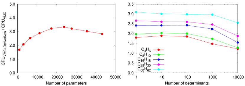
Figure 6: Cost per Monte Carlo step of computing a complete set of derivatives of the wave function and local energy relative to a VMC run where only the energy is calculated. Left: increasing number of variational parameters for the series $\text{C}_{n}\text{H}_{n+2}$ with $n$ between 4 and 44 (reproduced from Ref. [13]). Right: increasing number of determinants in the Jastrow-Slater wave function for $\text{C}_{n}\text{H}_{n+2}$ with $n$ between 4 and 60 (reproduced from Ref. [14]).

With all the derivatives of the wave function and the corresponding local quantities at hand, the next step is to use them for the optimization of the wave function. The use of wave functions with a large number of parameters requires efficient algorithms and the two most commonly used approaches, the linear method and the stochastic reconfiguration method, are discussed in the following. We will begin with the simpler case of the optimization in the ground state (or an excited state which is energetically the lowest for a given symmetry).

Stochastic Reconfiguration Method

In the stochastic reconfiguration (SR) method [65, 66], one starts from a given wave function, $\Psi$, and obtains an improved state by applying the operator $(1-\tau\hat{H})$, namely, a first-order expansion of the operator $e^{-\tau\hat{H}}$ used in DMC. The new state is then projected in the space spanned by the current wave function and its derivatives, $\{\Psi_{i}\}=\{\Psi,\partial_{i}\Psi\}$ as

$$\sum_{j=0}^{N_{p}}\delta p_{j}|\Psi_{j}\rangle=\hat{P}^{\text{SR}}(1-\tau\hat{H})|\Psi\rangle\,,$$ (26)

where $N_{p}$ is the number of wave function parameters and $\Psi_{0}=\Psi$. By taking the internal product with $\langle\Psi_{i}|$ and eliminating the scaling $\delta p_{0}$ through the $i=0$ equation, one derives a set of equations for $i=1,\ldots,N_{p}$, which can be written in matrix notation as

$$\bar{\mathbf{S}}\,\delta\mathbf{p}=-\frac{\tau}{2}\mathbf{g}\,,$$ (27)

where $\mathbf{g}$ is the gradient of the energy with respect to the parameters,

$$g_{i}=2\left[\frac{\langle\Psi_{i}|\hat{H}|\Psi\rangle}{\langle\Psi|\Psi\rangle}-E_{\mathrm{v}}\frac{\langle\Psi_{i}|\Psi\rangle}{\langle\Psi|\Psi\rangle}\right]\equiv\partial_{i}E_{\mathrm{v}}\,,$$ (28)

and $\bar{\mathbf{S}}$ is related to the overlap matrix between the derivatives, $\mathbf{S}$, as

$$\bar{S}_{ij}=\frac{\langle\Psi_{i}|\Psi_{j}\rangle}{\langle\Psi|\Psi\rangle}-\frac{\langle\Psi_{i}|\Psi\rangle}{\langle\Psi|\Psi\rangle}\frac{\langle\Psi|\Psi_{j}\rangle}{\langle\Psi|\Psi\rangle}\equiv S_{ij}-S_{i0}S_{0j}$$ (29)

With an appropriate choice of $\tau$, a new set of parameters can be determined as $p^{\prime}_{i}=p_{i}+\delta p_{i}$ and the procedure iterated until convergence. Therefore, the SR method is like a Newton approach where one follows the downhill gradient of the energy, using however the matrix $\bar{\mathbf{S}}$ instead of the Hessian of the energy. Even though the method can display a slow convergence since $\tau$ scales like the inverse of the energy range spanned by the wave function derivatives [67], it was recently employed to successfully optimize very large numbers of parameters [14, 15]. We will come back to this point when discussing the linear method below.

In a VMC run of SR optimization, one needs to compute the gradient and the overlap matrix ${\mathbf{S}}$ by sampling the distribution $\rho$ given by the square of the current wave function (Eq. 2) as

$$S_{ij} = \frac{\langle\Psi_{i}|\Psi_{j}\rangle}{\langle\Psi|\Psi\rangle}=\frac{\int\Psi_{i}(\mathbf{R})\Psi_{j}(\mathbf{R})\mathrm{d}\mathbf{R}}{\int\Psi(\mathbf{R})^{2}\mathrm{d}\mathbf{R}}$$ (30)

$$= \int\frac{\Psi_{i}(\mathbf{R})}{\Psi(\mathbf{R})}\frac{\Psi_{j}(\mathbf{R})}{\Psi(\mathbf{R})}\rho(\mathbf{R})\mathrm{d}\mathbf{R}\approx\frac{1}{M}\sum_{k}^{M}\frac{\Psi_{i}(\mathbf{R}_{k})}{\Psi(\mathbf{R}_{k})}\frac{\Psi_{j}(\mathbf{R}_{k})}{\Psi(\mathbf{R}_{k})}\,.$$

For large number of parameters, not only the storage of this matrix becomes problematic but also its calculation whose cost scales as $\mathcal{O}(MN_{p}^{2})$. However, if we use a conjugate gradient method to solve the linear equations (27), we only need to repeatedly evaluate ${\mathbf{S}}$ acting on a trial vector of parameter variations as

$$\sum_{j=1}^{N_{p}}{S}_{ij}\delta p_{j}=\frac{1}{M}\sum_{k}^{M}\frac{\Psi_{i}(\mathbf{R}_{k})}{\Psi(\mathbf{R}_{k})}\sum_{j=1}^{N_{p}}\frac{\Psi_{j}(\mathbf{R}_{k})}{\Psi(\mathbf{R}_{k})}\,\delta p_{j}\,,$$ (31)

where the order of the sums in the last expression has been swapped [68]. Therefore, if we compute and store the $M\times N_{p}$ matrix of the ratios $\Psi_{i}(\mathbf{R}_{k})/\Psi(\mathbf{R}_{k})$ during the Monte Carlo run, we can reduce the memory requirements by exploiting the intrinsic parallelism of Monte Carlo simulations: we can employ a small $M$ per core and increase instead the number of cores to obtain the desired statistical accuracy. The computational cost of solving the SR equations is also reduced to $\mathcal{O}(N_{\text{CG}}MN_{p})$, where $N_{\text{CG}}$ is the number of conjugate gradient steps, which we have found to be several orders of magnitude smaller than the number of parameters in recent optimization of large determinantal expansions [14, 15].

Linear Method

The linear optimization method is related to the so-called super configuration interaction (super-CI) approach used in quantum chemistry to optimize the orbital parameters in a multi-determinant wave function. The starting point is the normalized wave function,

$$|\bar{\Psi}\rangle=\frac{1}{\sqrt{\langle\Psi|\Psi\rangle}}|\Psi\rangle\,,$$ (32)

which we expand to first order in the parameter variations around the current values in the basis of the current wave function and its derivatives, $\{\bar{\Psi}_{i}\}=\{\bar{\Psi},\partial_{i}\bar{\Psi}\}$ with $\bar{\Psi}_{0}=\bar{\Psi}$. The important advantage of working with the “barred” functions is that they are orthogonal to the current wave function since

$$|\bar{\Psi}_{i}\rangle=\frac{1}{\sqrt{\langle\Psi|\Psi\rangle}}\big{(}|\Psi_{i}\rangle-\frac{\langle\Psi|\Psi_{i}\rangle}{\langle\Psi|\Psi\rangle}|\Psi\rangle\big{)}\,,$$ (33)

which has been found to yield better (non-linear) parameter variations and a more robust optimization than simply using the derivatives of the wave function.

The change of the parameters $\delta\mathbf{p}$ is then determined by minimizing the expectation value of the Hamiltonian on the linearized wave function in the basis $\{\bar{\Psi}_{i}\}$, which leads to the generalized eigenvalue equations:

$$\sum_{j=0}^{N_{p}}\bar{H}_{ij}\delta p_{j}=E_{\text{lin}}\sum_{j=0}^{N_{p}}\bar{S}_{ij}\delta p_{j}\,,$$ (34)

where $\bar{H}_{ij}=\langle\bar{\Psi}_{i}|\hat{H}|\bar{\Psi}_{j}\rangle$ and $\bar{S}_{ij}=\langle\bar{\Psi}_{i}|\bar{\Psi}_{j}\rangle$. We note that the overlap $\bar{\mathbf{S}}$ is equivalent to the expression introduced above in the SR scheme (Eq. 29). A new set of parameters can be generated as $p_{i}^{\prime}=p_{i}+\delta p_{i}/\delta p_{0}$ and the algorithm iterated until convergence. Importantly, in a Monte Carlo run, the matrix $\bar{\mathbf{H}}$ will not be symmetric for a finite sample and a non-obvious finding is that the method greatly benefits from reduced fluctuations if one does not symmetrize the Hamiltonian matrix, as originally shown by Nightingale and Melik-Alaverdian for the optimization of the linear parameters [32]. Other important modifications can be introduced to further stabilize the approach and improve the convergence as discussed in Ref. [7].

It is simple to recognize that, at convergence, the linear method leads to an optimal energy if we express explicitly the secular equations above in matrix form as

$$\begin{pmatrix}E_{\mathrm{v}}&\frac{1}{2}g^{\text{T}}\\ \frac{1}{2}g&\bar{\mathbf{H}}\end{pmatrix}\begin{pmatrix}\delta p_{0}\\ \delta\mathbf{p}\end{pmatrix}=E_{\text{lin}}\begin{pmatrix}1&0\\ 0&\bar{\mathbf{S}}\end{pmatrix}\begin{pmatrix}\delta p_{0}\\ \delta\mathbf{p}\end{pmatrix}\,,$$ (35)

where we have used that $\bar{H}_{00}=\langle\bar{\Psi}|\hat{H}|\bar{\Psi}\rangle$ is the current energy and the elements of the first column and row, $\bar{H}_{i0}=\langle\bar{\Psi}_{i}|\hat{H}|\bar{\Psi}\rangle$ and $\bar{H}_{0i}=\langle\bar{\Psi}|\hat{H}|\bar{\Psi}_{i}\rangle$, respectively, are both mathematically equal to the components of the energy gradient (Eq. 28). Therefore, when the wave function parameters are optimal, the variations with respect to the current wave function will no longer couple to it ($\delta p_{i}=0$) and the $\bar{H}_{i0}$ and $\bar{H}_{0i}$ elements must therefore become zero. This directly implies that the gradient of the energy with respect to the parameters is identically zero.

To further understand how the linear method is related to other optimization schemes, one can recast its equations as a Newton method [69]:

$$(\mathbf{A}+\alpha\bar{\mathbf{S}})\delta\mathbf{p}=-\frac{1}{2}\mathbf{g}\,,$$ (36)

where $\mathbf{A}=\bar{\mathbf{H}}-E_{\mathrm{v}}\bar{\mathbf{S}}$ and $\alpha=E_{\mathrm{v}}-E_{\text{lin}}>0$. Therefore, the parameters are varied along the downhill gradient of the energy with the use of an approximate Hessian $\mathbf{A}$ level-shifted by the positive definite matrix $\alpha\bar{\mathbf{S}}$. The presence of the latter renders the optimization more stable and effective than the actual Newton method even when the exact Hessian matrix is used. While the linear method is in principle significantly more efficient than for instance the SR approach, we find that its stochastic realization suffers from large fluctuations in the elements of $\bar{\mathbf{H}}$ when one optimizes the orbital parameters or the linear coefficients of particularly extended multi-determinant wave functions (where the derivatives are very different from the actual wave function used in the sampling). As a result, the optimization requires long VMC runs to achieve reliable variations in the parameters or a large shift added to the diagonal elements of $\bar{\mathbf{H}}$ (except $\bar{H}_{00}$) [7] to stabilize the procedure. In these cases, we find that the SR scheme, which only makes use of the $\bar{\mathbf{S}}$ matrix, is more robust and efficient since it allows less strict requirements on the error bars.

Finally, we note that, as in the SR scheme, it is possible to avoid to explicitly construct the full matrices $\bar{\mathbf{H}}$ and $\bar{\mathbf{S}}$: one stores the local quantities $\Psi_{i}(\mathbf{R})/\Psi(\mathbf{R})$ and $\hat{H}\Psi_{i}(\mathbf{R})/\Psi(\mathbf{R})$ in the Monte Carlo run and uses for instance a generalized Davidson algorithm to find the eigenvectors where only matrix-vector products with trial vectors are evaluated, significantly reducing the computational and memory requirements [68].

5 Excited States

For excited states of a different symmetry than the ground state, one can construct a trial wave function of the desired space and spin symmetry (with an appropriate choice of the determinantal component) and apply either the SR or the linear method to minimize the energy in VMC, subsequently refining the calculation in DMC. For excited states which are energetically not the lowest in their symmetry class, one can instead follow different routes as in other quantum chemistry methods to find an accurate excited-state wave function. We will begin to describe the possibilities within energy minimization and then consider optimization schemes targeting the variance of the energy which has a minimum for each eigenstate of the Hamiltonian.

1 Energy-based methods

While the linear method is generally employed for ground-state wave function optimizations, it is in fact possible to use it in a state-specific manner for the optimization of excited states [70]. One can target a higher-energy state and linearize the problem with respect to the chosen state. Solving a generalized eigenvalue problem as in Eq. 35 will yield lower energy roots as well as the state of interest. The resulting wave function will be only approximately orthogonal to the lower ones since orthogonality is only imposed in the basis of the variations of the optimal target wave function with respect to the parameters. Furthermore, since following such a higher root leads to the optimization of a saddle point in parameter space, the procedure may exhibit convergence problems so that the parameters do not converge to the desired state. One may also observe flipping of the roots: As the optimization proceeds the optimized excited target state can obtain a lower eigenvalue than the unoptimized ground state. Such problems will be particularly severe in case of close degeneracy as in proximity of conical intersection regions.

A different route to optimize multiple states of the same symmetry lies in the generalization of state-average (SA) approaches to QMC [9]. We start from a set of Jastrow-Slater wave functions for the multiple states that are constructed as linear combinations of determinants multiplied by a Jastrow factor as

$$\Psi^{I}=\mathcal{J}\sum_{k}c_{k}^{I}D_{k}\,,$$ (37)

where the index $I$ labels the states. The wave functions of the different states are therefore characterized by different linear coefficients $c_{i}^{I}$ but share a common set of orbitals and the Jastrow factor $\mathcal{J}$.

The optimal linear coefficients $c_{i}^{I}$ can be easily determined through the solution of the generalized eigenvalue equations

$$\sum_{j}H_{ij}c_{j}^{I}=E_{I}\sum_{j}S_{ij}c_{j}^{I}\,,$$ (38)

where the matrix elements are here given by

$$H_{ij}=\langle\mathcal{J}D_{i}|\hat{H}|\mathcal{J}D_{j}\rangle\ \ \ \text{and}\ \ \ S_{ij}=\langle\mathcal{J}D_{i}|\mathcal{J}D_{j}\rangle\,,$$ (39)

and are computed in a VMC run, where we do not symmetrize the Hamiltonian matrix for finite Monte Carlo sampling to reduce the fluctuations of the parameters as discussed above for the general linear method. After diagonalization of Eq. 38, the optimal linear coefficients are obtained and, at the same time, orthogonality between the individual states is automatically enforced.

To obtain a robust estimate of the linear coefficients of multiple states, it is important that the distribution sampled to evaluate $H_{ij}$ and $S_{ij}$ has a large overlap with all states of interest (and all lower lying states). A suitable guiding wave function can for instance be constructed as

$$\Psi_{g}=\sqrt{\sum_{I}|\Psi_{I}|^{2}}\,,$$ (40)

and the distribution $\rho_{g}$ in the VMC run defined as the square of this guiding function. The matrix elements $S_{ij}$ (and, similarly, $H_{ij}$) are then evaluated in the Monte Carlo run as

$$\frac{S_{ij}}{\langle\Psi_{g}|\Psi_{g}\rangle} = \frac{\int\mathcal{J}D_{i}(\mathbf{R})\mathcal{J}D_{j}(\mathbf{R})\mathrm{d}\mathbf{R}}{\int\Psi_{g}^{2}(\mathbf{R})\mathrm{d}\mathbf{R}}=\int\frac{\mathcal{J}D_{i}(\mathbf{R})}{\Psi_{g}(\mathbf{R})}\frac{\mathcal{J}D_{j}(\mathbf{R})}{\Psi_{g}(\mathbf{R})}\rho_{g}(\mathbf{R})\mathrm{d}\mathbf{R}$$ (41)

$$\approx \frac{1}{M}\sum_{k}^{M}\frac{\mathcal{J}D_{i}(\mathbf{R}_{k})}{\Psi_{g}(\mathbf{R}_{k})}\frac{\mathcal{J}D_{j}(\mathbf{R}_{k})}{\Psi_{g}(\mathbf{R}_{k})}\,.$$

We note that we can introduce the denominator $\langle\Psi_{g}|\Psi_{g}\rangle$ if we simply divide by it both sides of Eq. 38.

As done in state-average multi-configurational approaches to obtain a balanced description of the states of interest, one can optimize the non-linear parameters of the orbitals and the Jastrow factor by minimizing the state-average energy

$$E^{\text{SA}}=\sum_{I}w_{I}\frac{\langle\Psi^{I}|\hat{H}|\Psi^{I}\rangle}{\langle\Psi^{I}|\Psi^{I}\rangle}\,,$$ (42)

with the weights of the states $w_{I}$ kept fixed and $\sum_{I}w_{I}=1$. The gradient of the SA energy can be rewritten as

$$g^{\text{SA}}_{i}=\sum_{I}w_{I}{\langle\bar{\Psi}^{I}_{i}|\hat{H}|\Psi^{I}\rangle}\,,$$ (43)

where, similarly to Eq. 33, we have introduced for each state the variations, ${|\Psi_{i}^{I}\rangle=|\partial_{i}\Psi^{I}\rangle}$, and the corresponding “barred” functions orthogonal to the current state $|\Psi^{I}\rangle$:

$$|\bar{\Psi}_{i}^{I}\rangle=\frac{1}{\sqrt{\langle\Psi^{I}|\Psi^{I}\rangle}}\big{(}|\Psi_{i}^{I}\rangle-\frac{\langle\Psi^{I}|\Psi^{I}_{i}\rangle}{\langle\Psi^{I}|\Psi^{I}\rangle}|\Psi^{I}\rangle\big{)}\,.$$ (44)

The variations in the parameters can be obtained as the lowest-energy solution of the generalized eigenvalue equation in analogy to the linear method for the ground state,

$$\begin{pmatrix}E^{\text{SA}}&\frac{1}{2}(g^{\text{SA}})^{\text{T}}\\ \frac{1}{2}g^{\text{SA}}&\bar{\mathbf{H}}^{\text{SA}}\end{pmatrix}\begin{pmatrix}\delta p_{0}\\ \delta\mathbf{p}\end{pmatrix}=E\begin{pmatrix}1&0\\ 0&\bar{\mathbf{S}}^{\text{SA}}\end{pmatrix}\begin{pmatrix}\delta p_{0}\\ \delta\mathbf{p}\end{pmatrix}\,.$$ (45)

The state-average matrix elements are defined as

$$\bar{H}_{ij}^{\text{SA}}=\sum_{I}w_{I}\frac{\langle\bar{\Psi}^{I}_{i}|\hat{H}|\bar{\Psi}^{I}_{j}\rangle}{\langle\bar{\Psi}^{I}|\bar{\Psi}^{I}\rangle}\,,$$ (46)

and an analogous expression for $\bar{S}_{ij}^{\text{SA}}$ is introduced. To compute these matrix elements in VMC, we perform a single run sampling the square of a guiding wave function $\Psi_{g}$ (Eq. 40) and compute the numerators and denominators in the matrix expressions for all relevant states. We note that the state-average equations (Eq. 45) are not obtained by minimizing a linearized expression of the SA energy (Eq. 42) but are simply inspired by the single-state case. However, since the first row and column in Eq. 45 are given by the gradient of the SA energy, at convergence, the optimal parameters minimize the SA energy. We find that the use of these state-average Hamiltonian and overlap matrices leads to a similar convergence behavior as the linear method for a single state.

Following this procedure, the algorithm alternates between the minimization of the linear and the non-linear parameters until convergence is reached. The obtained energy $E_{\text{SA}}$ is stationary with respect to variations of all parameters while the energies of the individual states, $E_{I}$, are only stationary with respect to the linear but not the orbital and Jastrow parameters. If the ground state and the target excited state should be described by very different orbitals, a state-specific approach may yield more accurate energies.

2 Time-dependent linear-response VMC

A very different approach to the computation of multiple excited states is a VMC formulation of linear-response theory [71]. Given a starting wave function $\Psi$ with optimal parameters $\mathbf{p}_{0}$, a time-dependent perturbation $\hat{V}(t)$ is introduced in the Hamiltonian $\hat{H}$ with the coupling constant $\gamma$ as

$$\hat{H}(t)=\hat{H}+\gamma\hat{V}(t)\,,$$ (47)

so that the ground-state wave function itself becomes time-dependent as the variational parameters $\mathbf{p}(t)$ evolve in time. It is convenient to work with a wave function subject to an intermediate normalization,

$$|\bar{\Psi}(t)\rangle=\frac{|\Psi(t)\rangle}{\left<\Psi_{0}|\Psi(t)\right>}\,,$$ (48)

where the starting wave function $\Psi_{0}\equiv\Psi$ is taken to be normalized. This choice leads to wave function variations to first and second order that are orthogonal to the current optimal wave function $\Psi_{0}$.

At each time $t$, one can apply the Dirac-Frenkel variational principle to obtain the parameters $\mathbf{p}(t)$ as

$$\frac{\partial}{\partial p_{i}^{*}}\frac{\langle\bar{\Psi}(t)|\hat{H}(t)-i\frac{\partial}{\partial t}|\bar{\Psi}(t)\rangle}{\langle\bar{\Psi}(t)|\bar{\Psi}(t)\rangle}=0,$$ (49)

where the parameters can now in general be complex. To apply this principle to linear order in $\gamma$, the wave function is expanded to second order in $\delta\mathbf{p}(t)$ around $\mathbf{p}_{0}$:

$$|\bar{\Psi}(t)\rangle=|\bar{\Psi}_{0}\rangle+\sum_{i}\delta p_{i}(t)|\bar{\Psi}_{i}\rangle+\frac{1}{2}\sum_{ij}\delta p_{i}(t)\delta p_{j}(t)|\bar{\Psi}_{ij}\rangle\,,$$ (50)

with $|\bar{\Psi}_{i}\rangle=|\partial_{i}\bar{\Psi}\rangle$ and $|\bar{\Psi}_{ij}\rangle=|\partial_{i}\partial_{j}\bar{\Psi}\rangle$ computed at the parameters $\mathbf{p}_{0}$. These can be explicitly written as

$$|\bar{\Psi}_{i}\rangle\ = |\Psi_{i}\rangle-\langle\Psi_{0}|\Psi_{i}\rangle|\Psi_{0}\rangle$$

$$|\bar{\Psi}_{ij}\rangle = |\Psi_{ij}\rangle-\langle\Psi_{0}|\Psi_{i}\rangle|\Psi_{j}\rangle-\langle\Psi_{0}|\Psi_{j}\rangle|\Psi_{i}\rangle$$ (51)

$$+ \left(2\langle\Psi_{0}|\Psi_{i}\rangle\langle\Psi_{0}|\Psi_{j}\rangle-\langle\Psi_{0}|\Psi_{ij}\rangle\right)|\Psi_{0}\rangle\,,$$

where we use the same notation as above for the derivatives of $\Psi$, namely, $|\Psi_{i}\rangle=|\partial_{i}\Psi\rangle$ and $|\Psi_{ij}\rangle=|\partial_{i}\partial_{j}\Psi\rangle$. Inserting this wave function in Eq. 49 and keeping only the first-order terms in $\delta\mathbf{p}(t)$, in the limit of $\gamma\rightarrow 0$, one obtains

$$\mathbf{A}\,\delta\mathbf{p}(t)+\mathbf{B}\,\delta\mathbf{p}(t)^{*}=i\bar{\mathbf{S}}\,\frac{\partial\delta\mathbf{p}(t)}{\partial t}\,,$$ (52)

with the matrix elements $A_{ij}=\langle\bar{\Psi}_{i}|\hat{H}-E_{0}|\bar{\Psi}_{j}\rangle=\bar{H}_{ij}-E_{0}\bar{S}_{ij}$ and $B_{ij}=\langle\bar{\Psi}_{ij}|\hat{H}|\Psi_{0}\rangle$. If we search for an oscillatory solution,

$$\delta\mathbf{p}(t)=\mathbf{X}_{n}e^{-i\omega_{n}t}+\mathbf{Y}_{n}^{*}e^{i\omega_{n}t}\,,$$ (53)

with $\omega_{n}$ an excitation energy and $\mathbf{X}_{n}$ and $\mathbf{Y}_{n}$ the response vectors, we obtain the well-known linear-response equations, here formulated as a non-Hermitian generalized eigenvalue equation,

$$\begin{pmatrix}\mathbf{A}&\mathbf{B}\\ \ \mathbf{B}^{*}&\ \mathbf{A}^{*}\end{pmatrix}\begin{pmatrix}\mathbf{X}_{n}\\ \mathbf{Y}_{n}\end{pmatrix}=\omega_{n}\begin{pmatrix}\bar{\mathbf{S}}&\mathbf{0}\\ \mathbf{0}&-\bar{\mathbf{S}}^{*}\end{pmatrix}\begin{pmatrix}\mathbf{X}_{n}\\ \mathbf{Y}_{n}\end{pmatrix}\,.$$ (54)

Neglecting $\mathbf{B}$ leads to the Tamm-Dancoff approximation,

$$\mathbf{A}\mathbf{X}_{n}=\omega_{n}\bar{\mathbf{S}}\mathbf{X}_{n}\,,$$ (55)

which is equivalent to the generalized eigenvalue equations of the linear method (Eq. 35) for an optimized ground-state wave function (when the gradients of the energy are therefore zero):

$$\bar{\mathbf{H}}\mathbf{X}_{n}=(\omega_{n}+E_{0})\bar{\mathbf{S}}\mathbf{X}_{n}\,.$$ (56)

The energy $E_{0}$ is the variational energy, $E_{\mathrm{v}}$, for the optimized ground state. Therefore, upon optimization of the ground-state wave function in the linear method, we can simply use the higher roots resulting from the diagonalization of the equations to estimate the excitation energies as $\omega_{n}=(E_{\text{lin}})_{n}-E_{0}$ together with the oscillator strengths [71].

The time-dependent linear-response VMC approach has so far only been applied to the excitations of the beryllium atom within the Tamm-Dancoff approximation and with a simple single-determinant Jastrow-Slater wave function [71]. These calculations represent an interesting proof of principle that multiple excitations of different space and spin symmetry can be readily obtained after optimizing the ground-state wave function. A systematic investigation with multi-configurational wave functions is needed to fully access the quality of the approach, also beyond the Tamm-Dancoff approximation.

3 Variance-based methods

Variance minimization is a different approach to optimize the wave function compared to the methods described so far, which allows in principle to optimize excited states in a state-specific fashion. The target quantity for the minimization is the variance of the energy:

$$\sigma_{\mathrm{v}}^{2}=\frac{\langle\Psi|(\hat{H}-E_{\mathrm{v}})^{2}|\Psi\rangle}{\langle\Psi|\Psi\rangle}=\frac{\int\Psi^{2}(\mathbf{R})(E_{\mathrm{L}}(\mathbf{R})-E_{\mathrm{v}})^{2}\mathrm{d}\mathbf{R}}{\int\Psi^{2}(\mathbf{R})\mathrm{d}\mathbf{R}}\,.$$ (57)

While the (global) minimum of the variational energy is only obtained for the ground state, the variance has a known minimum of zero for each eigenstate of the Hamiltonian. The optimization of the variance can be performed using either a Newton approach with an approximate expression of the Hessian of the variance [5] or reformulated as a generalized eigenvalue problem, namely, a linear method for the optimization of the variance [69]. For excited states, the initial guess of the trial wave function might however be very important to select a specific state and ensure that the minimization of the variance leads to the correct local minimum.

More robust state-specific variational principles for excited states can be formulated so that the optimization of the excited state yields a minimum close to an initial target energy. A simple possibility is to substitute the wave-function-dependent average energy in $\sigma_{\mathrm{v}}$ with a guess value $\omega$ as in

$$\sigma^{2}_{\omega}=\frac{\langle\Psi|(\hat{H}-\omega)^{2}|\Psi\rangle}{\langle\Psi|\Psi\rangle}\equiv(E_{\mathrm{v}}-\omega)^{2}+\sigma_{\mathrm{v}}^{2}\,,$$ (58)

as it was done in the early applications of variance minimization on a fixed Monte Carlo sample [72], where $\omega$ was chosen equal to a target value at the beginning of the optimization and then adjusted to the current best energy. If one updates $\omega$ in this manner, minimizing $\sigma_{\omega}$ is equivalent to minimizing $\sigma_{\mathrm{v}}$.

Alternatively, minimization of the variance can also be achieved by optimizing the recently proposed functional $\Omega$ defined as

$$\Omega=\frac{\langle\Psi|\omega-\hat{H}|\Psi\rangle}{\langle\Psi|(\omega-\hat{H})^{2}|\Psi\rangle}=\frac{\omega-E_{\mathrm{v}}}{(\omega-E_{\mathrm{v}})^{2}+\sigma_{\mathrm{v}}}\,,$$ (59)

where $\omega$ is adjusted during the optimization to be equal to the current value of $E_{\mathrm{v}}-\sigma_{\mathrm{v}}$ [10, 11]. While the functional has formally a minimum for a state with energy directly above $\omega+\sigma_{\mathrm{v}}$, keeping $\omega$ fixed would lead to lack of size consistency in the variational principle [11]. Therefore, after some initial iterations, $\omega$ is gradually varied to match the current value of $E_{\mathrm{v}}-\sigma_{\mathrm{v}}$ required to achieve variance minimization. As in the case of the energy and the variance, this functional can be optimized in VMC through a generalization of the linear method [10, 30].

6 Applications to excited states of molecular systems

The status of excited-state quantum Monte Carlo calculations closely parallels the methodological developments that have characterized the last decade as we have outlined above in the context of wave function optimization. Since the early applications to excited states, QMC methods were mainly employed as a tool to compute vertical excitation energies and validate results of more approximate methods. Input from other – sometimes much less accurate – quantum chemical approaches was however then used for the construction of the wave function, whose determinant component was generally not optimized in the presence of the Jastrow factor. The success of the calculation was therefore often heavily relying on the ability of DMC to overcome possible shortcomings of the chosen trial wave function. This must be contrasted to the recent situation of VMC having matured to a fully self-consistent method as regards the wave function and the geometry with a rich ecosystem of tools ranging from basis sets and pseudopotentials to multi-scale formulations.

One of the first QMC computations of two states of the same symmetry was carried out for the H₂ molecule [73]: the wave function was obtained from a multi-reference calculation and DMC was shown to be able in this case to correct for the wave function bias. Over the subsequent years, a number of studies of vertical excitation energies were carried out with this basic recipe, namely, performing DMC calculations on a given simple wave function obtained at a lower level of theory [74, 75, 76, 77, 78, 79, 80, 81, 82, 83]. Some of these early excited-state calculations were in fact pioneering as they were applied to remarkably large systems such as silicon and carbon nanoclusters with more than hundred atoms [74, 76, 79]. Given the size of the systems, the choice of excited-state wave function was then very simple and consisted of a single determinant correlated with a Jastrow factor and constructed with the HOMO and LUMO orbitals from a density functional theory (DFT) calculation. Nevertheless, the resulting DMC excitation energies clearly represented an improvement on the time-dependent DFT values and captured much of the qualitative physics of the problem. Even though doubts on the validity of this simplistic recipe [82, 83] led researchers to investigate the use of orbitals and pseudopotentials obtained with different density functionals [79] as well as a multi-determinant description [83], a rather heuristic approach erring on the side of computational saving characterized excited-state calculations in this earlier period.

More recently, the development of algorithms for wave function optimizations in a state-specific or state-average fashion has allowed us to better understand the proper ingredients in an excited-state QMC calculation through the study of simple but challenging molecules. In particular, it has become apparent that large improvements in the accuracy of both VMC and DMC excited states can be achieved by optimizing the determinantal component in the presence of the Jastrow factor at the VMC level [67, 61, 9, 70, 84, 64]. For instance, accurate excitations for low-lying states of ethene can only be obtained if the orbitals derived from a complete-active-space self-consistent-field (CASSCF) calculation are reoptimized in the presence of the Jastrow factor to remove spurious valence-Rydberg mixing in the final DMC energies [67]. The analysis of various small organic molecules reveals that the use of simplistic wave functions such as a HOMO-LUMO Hartree-Fock or a configuration-interaction-singles ansatz may lead to significant errors also in DMC [61]. An investigation of the ground and excited states of methylene shows that the optimization of all variational parameters reduces the dependency of both VMC and DMC on the size of the active space employed for the trial wave function as shown in Fig. 7 [70]. In general, while a minimal requirement is to optimize the linear coefficients together with the Jastrow factor, the optimization of the orbitals is highly recommended, especially if one employs a truncated expansion in computing the excitation energies. Furthermore, evidence has been given that the optimization of excited-state geometries requires the optimization of all wave function parameters in order to obtain accurate gradients and, consequently, geometries [63]. Finally, by construction, linear-response VMC depends strongly on the quality of the ground-state wave function for the description of excited states and, therefore benefits considerably from orbital optimization in the ground state [71].

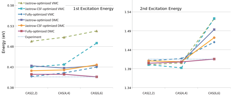
Figure 7: Convergence of VMC and DMC adiabatic excitation energies for the first and second excited states of methylene with increasing CAS size. Three levels of optimization have been used for the wave function: Jastrow, Jastrow and linear coefficients, and all parameters. Adapted from Ref. [70].

While these and other examples of excited-state QMC calculations clearly illustrate the importance of using wave functions with an adequate description of static correlation and consistently optimized in VMC, they also demonstrate the robustness of QMC approaches and some of their advantages with respect to standard multi-configurational methods. In particular, the VMC and DMC excitations are well converged already when very few determinants of a CAS expansion are kept in the determinantal component of the wave function [9, 84]. Furthermore, the demands on the size of the basis set are also less severe and one can obtain converged excitation energies with rather small basis sets [63, 24, 64]. We note that most of the recent QMC calculations for excited states have attempted to achieve a balanced static description of the states of interest either by employing a CAS in the determinantal component or a truncated multi-reference ansatz where one keeps the union of the configuration state functions resulting from an appropriate truncation scheme (e.g. the sum of the squared coefficients being similar for all states). Interestingly, matching the variance of the states has recently been put forward as a more robust approach to achieve a balanced treatment of the states in the computation of excitation energies [85, 30].

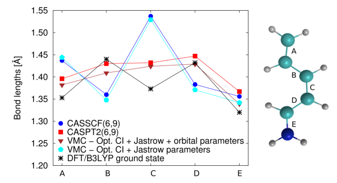
Figure 8: Planar excited-state geometry of a retinal protonated Schiff base model optimized with CASSCF, second-order perturbation theory (CASPT2), and VMC. Adapted from Ref. [63].

The ability to optimize geometries even in the ground states has been a very recent achievement for QMC methods, so most QMC calculations also outside the Franck-Condon region have been performed on geometries obtained at a different level of theory [61, 86, 87, 70, 88, 83, 30]. Nevertheless, these investigations have led to very promising results, showing interesting prospects for the application of QMC to geometry relaxations in the excited state, where most quantum chemical methods either lack the required accuracy or are computationally prohibitive due to their scaling with system size. For example, QMC was successfully employed to assess the accuracy of various time-dependent DFT methods in describing the photochemisty of oxirane through exploration of multiple excited-state potential energy surfaces, also in proximity of conical intersection regions [86, 87]. Another application demonstrating the very good performance of DMC was the study of different conformers of azobenzene in the ground and excited states [88]. To the best of our knowledge, to date, the only few attempts to optimize an excited-state geometry via QMC gradients are our studies of the retinal protonated Schiff base model [63, 24] and benchmark calculations on small organic molecules in the gas phase [89] and in a polarizable continuum model [46]. As shown for the retinal minimal model in Fig. 8, the results are very encouraging as they demonstrate that the QMC structures relaxed in the excited state are in very good agreement with other highly-correlated approaches. As already mentioned, the VMC gradients are sensitive to the quality of the wave function and the orbitals must be reoptimized in VMC to obtain accurate results. Tests also indicate that the use of DMC gradients is not necessary as DMC cannot compensate for the use of an inaccurate wave function while it yields comparable results to VMC when the fully optimized wave function is employed.

Finally, we mention the recent developments of multi-scale methods in combination with QMC calculations for excited states. Multi-scale approaches are particularly relevant for the description of photoactive processes that can be traced back to a region with a limited number of atoms, examples being a chromophore in a protein or a solute in a solvent. While this locality enables us to treat the photoactive region quantum mechanically, excited-state properties can be especially sensitive to the environment (e.g. the polarity of a solvent or nearby residues of a protein), which cannot therefore be neglected but are often treated at lower level of theory. Multi-scale approaches are well-established in traditional quantum chemistry but represent a relatively new area of research in the context of QMC. First steps in this direction were made by combining VMC with a continuum solvent model, namely, the polarizable continuum model (PCM) [90]. The approach was used to investigate solvent effects on the vertical excitation energies of acrolein [44] and on the optimal excited-state geometries of a number of small organic molecules [46]. A notable advantage of VMC/PCM is that the interaction between the polarizable embedding and the solute is described self-consistently at the same level of theory. This stands for instance in contrast to perturbation approaches which include the interaction with the environment obtained self-consistently only at the zero-order level (e.g. CASSCF).

To achieve a more realistic description of the environment, a static molecular mechanics environment coupled via electrostatic interactions with the VMC or DMC chromophore was used to describe the absorption properties of the green fluorescent protein and rhodopsin [91, 92]. The limitations of such a non-polarizable embedding scheme led to further developments, replacing the static description with a polarizable one in a so-called VMC/MMpol approach [47]. The force field consists of static partial charges located at the positions of the atoms as well as atomic polarizibilities. These are used to compute induced dipoles in equilibrium with the embedded system at the level of VMC, which are then kept fixed in subsequent DMC calculations. The computation of the QMC excitation energies can be carried out for two polarization schemes: either the induced dipoles are determined for the ground state and used also for the excited state (polGS), or the excitation energy is computed in a state-specific manner as the difference between the ground- and excited-state energies both obtained self-consistently in equilibrium with the respective induced dipoles (polSS). As illustrated in Fig. 9, the vertical excitation energies of small molecules in water clusters depend strongly on the sophistication of the embedding scheme. Only the polarizable force field with two separate sets of induced dipoles for the ground and excited states leads to a very good agreement with the supermolecular excitation. Again, the QMC results agree with complete-active-space second-order perturbation theory (CASPT2) which however is found to be rather sensitive to the choice of the active space. The most sophisticated QMC embedding scheme has so far been realized using a wave-function-in-DFT method and including differential polarization effects through state-specific embedding potentials [45]. As in the case of the polSS approach, the use of different potentials in the ground and excited state is particularly important for excitations which involve large polarization effects due to a considerable rearrangement of the electron density upon excitation.

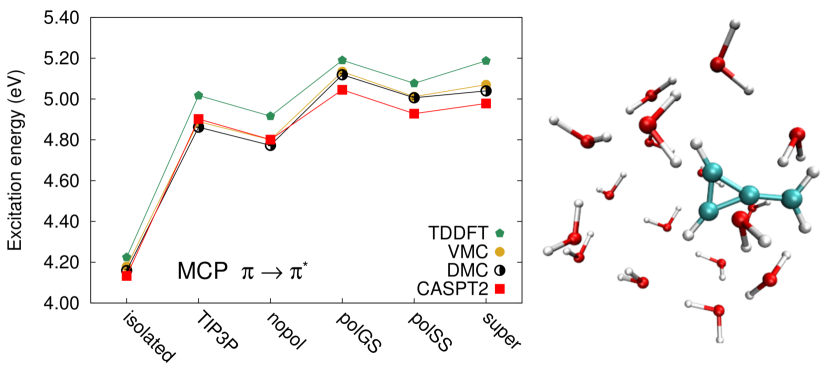
Figure 9: Energies of the $\pi\rightarrow\pi^{*}$ excitation of methylenecyclopropene in vacuum and embedded in a cluster of water molecules, computed with time-dependent DFT, CASPT2, VMC, and DMC. The water molecules are described with a static TIP3P force field and a MMpol approach with no polarization (nopol), with induced ground-state (polGS) and state-specific (polSS) dipoles, and in a supermolecular calculation (super). Adapted from Ref. [47].

7 Alternatives to diffusion Monte Carlo

In some of the applications we presented, VMC has been shown sufficient to provide accurate excited-state properties without the need to perform a DMC calculation. The reason is that the burden and complexity of the problem have now been moved from the DMC projection to the construction and optimization at the VMC level of sophisticated wave functions with many parameters. It is therefore natural to ask if there are alternatives to DMC, which do not require us to build and optimize complicated many-body wave functions.

The Cerperley-Bernu method [93] can in principle be used to compute the lowest-energy eigenstates and the corresponding relevant matrix elements by constructing a set of many-body basis states and improving upon them through the application of the imaginary-time projection operator also used in DMC. The Hamiltonian and overlap matrices are computed on these improved basis states during the projection and the eigenvalues and eigenstates are then obtained by solving this generalized eigenvalue problem. The method requires however that the fixed-node constraint is relaxed during the projection, and therefore amounts to an expensive “nodal-release” approach. The approach has been successfully applied to the computation of low-lying excitations of bosonic systems [32, 93] and has also been used to compute tens of excited states of the fermionic, high-pressure liquid hydrogen in order to estimate its electrical conductivity [94].

If we move beyond a continuum formulation of QMC, the auxiliary-field quantum Monte Carlo (AFQMC) method by Zhang and coworkers [95] represents a very distinct, feasible alternative to DMC. In this approach, the random walk is in a space of single-particle Slater determinants, which are subject to a fluctuating external potential. The fermion-sign problem appears here in the form of a phase problem and is approximately eliminated by requiring that the phase of the determinant remains close to the phase of a trial wave function. The method is more expensive than DMC but has been applied to a variety of molecular and extended systems (mainly in the ground state) and appears to be less plagued by the phase constraint as compared to the effect of the fixed-node approximation in DMC. A very recent review of AFQMC and its applications also to excited states can be found in Ref. [96].

Finally, we should mention another QMC approach in determinantal space, namely, the full configuration interaction quantum Monte Carlo method [97, 98] where a stochastic approach is used to select the important determinants in a full configuration interaction expansion. The method has been described in Chapter X together with its extension to excited states.

References

- [1] W. M. C. Foulkes, L. Mitas, R. J. Needs, and G. Rajagopal, “Quantum Monte Carlo simulations of solids,” Reviews of Modern Physics, vol. 73, pp. 33–83, Jan. 2001.
- [2] A. Lüchow, “Quantum Monte Carlo methods,” Wiley Interdisciplinary Reviews: Computational Molecular Science, vol. 1, no. 3, pp. 388–402, 2011.
- [3] B. M. Austin, D. Y. Zubarev, and W. A. Lester, “Quantum Monte Carlo and related approaches,” Chemical Reviews, vol. 112, pp. 263–288, Jan. 2012.
- [4] J. Hermann, D. Alfè, and A. Tkatchenko, “Nanoscale π–π stacked molecules are bound by collective charge fluctuations,” Nature Communications, vol. 8, p. 14052, Feb. 2017.
- [5] C. J. Umrigar and C. Filippi, “Energy and variance optimization of many body wave functions,” The Journal of Chemical Physics, vol. 94, p. 150201, 2005.
- [6] C. J. Umrigar, J. Toulouse, C. Filippi, S. Sorella, and R. G. Hennig, “Alleviation of the fermion-sign problem by optimization of many-body wave functions,” Physical Review Letters, vol. 98, no. 11, p. 110201, 2007.
- [7] J. Toulouse and C. J. Umrigar, “Optimization of quantum Monte Carlo wave functions by energy minimization,” The Journal of Chemical Physics, vol. 126, p. 084102, Feb. 2007.
- [8] L. Zhao and E. Neuscamman, “A blocked linear method for optimizing large parameter sets in variational Monte Carlo,” Journal of Chemical Theory and Computation, vol. 13, no. 6, pp. 2604–2611, 2017.
- [9] C. Filippi, M. Zaccheddu, and F. Buda, “Absorption spectrum of the green fluorescent protein chromophore: A difficult case for ab initio methods?,” Journal of Chemical Theory and Computation, vol. 5, pp. 2074–2087, Aug. 2009.
- [10] L. Zhao and E. Neuscamman, “An efficient variational principle for the direct optimization of excited states,” Journal of Chemical Theory and Computation, vol. 12, pp. 3436–3440, Aug. 2016.
- [11] J. A. R. Shea and E. Neuscamman, “Size consistent excited states via algorithmic transformations between variational principles,” Journal of Chemical Theory and Computation, vol. 13, pp. 6078–6088, Dec. 2017.
- [12] S. Sorella and L. Capriotti, “Algorithmic differentiation and the calculation of forces by quantum Monte Carlo,” The Journal of Chemical Physics, vol. 133, no. 23, p. 234111, 2010.
- [13] C. Filippi, R. Assaraf, and S. Moroni, “Simple formalism for efficient derivatives and multi-determinant expansions in quantum Monte Carlo,” The Journal of Chemical Physics, vol. 144, no. 19, p. 194105, 2016.
- [14] R. Assaraf, S. Moroni, and C. Filippi, “Optimizing the energy with quantum Monte Carlo: A lower numerical scaling for Jastrow–Slater expansions,” Journal of Chemical Theory and Computation, vol. 13, pp. 5273–5281, Nov. 2017.
- [15] M. Dash, S. Moroni, A. Scemama, and C. Filippi, “Perturbatively selected configuration-interaction wave functions for efficient geometry optimization in quantum Monte Carlo,” Journal of Chemical Theory and Computation, June 2018.
- [16] Y. Luo, A. Zen, and S. Sorella, “Ab initio molecular dynamics with noisy forces: Validating the quantum Monte Carlo approach with benchmark calculations of molecular vibrational properties,” The Journal of Chemical Physics, vol. 141, p. 194112, Nov. 2014.
- [17] A. Zen, Y. Luo, G. Mazzola, L. Guidoni, and S. Sorella, “Ab initio molecular dynamics simulation of liquid water by quantum Monte Carlo,” The Journal of Chemical Physics, vol. 142, p. 144111, Apr. 2015.
- [18] P. L. Rios, A. Ma, N. Drummond, M. Towler, and R. Needs, “Inhomogeneous backflow transformations in quantum Monte Carlo calculations,” Physical Review E, vol. 74, p. 066701, 2006.
- [19] M. Holzmann and S. Moroni, “Orbital-dependent backflow wave functions for real-space quantum Monte Carlo,” Physical Review B, vol. 99, p. 085121, Feb. 2019.
- [20] M. Casula and S. Sorella, “Geminal wave functions with Jastrow correlation: A first application to atom,” The Journal of Chemical Physics, vol. 119, p. 6500, 2003.
- [21] M. Casula, C. Attaccalite, and S. Sorella, “Correlated geminal wave function for molecules: An efficient resonating valence bond approach,” The Journal of Chemical Physics, vol. 121, p. 7110, 2004.
- [22] M. Bajdich, L. Mitas, L. Wagner, and K. Schmidt, “Pfaffian pairing and backflow wave functions,” Physical Review B, vol. 77, p. 115112, 2008.
- [23] F. Fracchia, C. Filippi, and C. Amovilli, “Size-extensive wave functions for quantum Monte Carlo: A linear scaling generalized valence bond approach,” Journal of Chemical Theory and Computation, vol. 8, pp. 1943–1951, June 2012.
- [24] H. Zulfikri, C. Amovilli, and C. Filippi, “Multiple-resonance local wave functions for accurate excited states in quantum Monte Carlo,” Journal of Chemical Theory and Computation, vol. 12, no. 3, pp. 1157–1168, 2016.
- [25] R. C. Clay and M. A. Morales, “Influence of single particle orbital sets and configuration selection on multideterminant wavefunctions in quantum Monte Carlo,” The Journal of Chemical Physics, vol. 142, p. 234103, June 2015.
- [26] M. C. Per and D. M. Cleland, “Energy-based truncation of multi-determinant wavefunctions in quantum Monte Carlo,” The Journal of Chemical Physics, vol. 146, p. 164101, Apr. 2017.
- [27] P. J. Robinson, S. D. Pineda Flores, and E. Neuscamman, “Excitation variance matching with limited configuration interaction expansions in variational Monte Carlo,” The Journal of Chemical Physics, vol. 147, p. 164114, Oct. 2017.
- [28] J. Kim, A. D. Baczewski, T. D. Beaudet, A. Benali, M. C. Bennett, M. A. Berrill, N. S. Blunt, E. J. L. Borda, M. Casula, D. M. Ceperley, S. Chiesa, B. K. Clark, R. C. Clay, K. T. Delaney, M. Dewing, K. P. Esler, H. Hao, O. Heinonen, P. R. C. Kent, J. T. Krogel, I. Kylänpää, Y. W. Li, M. G. Lopez, Y. Luo, F. D. Malone, R. M. Martin, A. Mathuriya, J. McMinis, C. A. Melton, L. Mitas, M. A. Morales, E. Neuscamman, W. D. Parker, S. D. P. Flores, N. A. Romero, B. M. Rubenstein, J. A. R. Shea, H. Shin, L. Shulenburger, A. F. Tillack, J. P. Townsend, N. M. Tubman, B. V. D. Goetz, J. E. Vincent, D. C. Yang, Y. Yang, S. Zhang, and L. Zhao, “QMCPACK: an open source ab initio quantum Monte Carlo package for the electronic structure of atoms, molecules and solids,” Journal of Physics: Condensed Matter, vol. 30, p. 195901, Apr. 2018.
- [29] A. Scemama, A. Benali, D. Jacquemin, M. Caffarel, and P.-F. Loos, “Excitation energies from diffusion Monte Carlo using selected configuration interaction nodes,” The Journal of Chemical Physics, vol. 149, p. 034108, July 2018.
- [30] S. D. Pineda Flores and E. Neuscamman, “Excited state specific multi-slater Jastrow wave functions,” The Journal of Physical Chemistry A, vol. 123, no. 8, pp. 1487–1497, 2019. PMID: 30702890.
- [31] R. Assaraf and M. Caffarel, “Zero-variance principle for Monte Carlo algorithms,” Physical Review Letters, vol. 83, p. 4682, 1999.
- [32] M. P. Nightingale and V. Melik-Alaverdian, “Optimization of ground- and excited-state wave functions and van der Waals clusters,” Physical Review Letters, vol. 87, no. 4, p. 043401, 2001.
- [33] R. Assaraf and M. Caffarel, “Zero-variance zero-bias principle for observables in quantum Monte Carlo: Application to forces,” The Journal of Chemical Physics, vol. 119, p. 10536, 2003.
- [34] J. Toulouse, R. Assaraf, and C. J. Umrigar, “Zero-variance zero-bias quantum Monte Carlo estimators of the spherically and system-averaged pair density,” The Journal of Chemical Physics, vol. 126, no. 244112, 2007.
- [35] C. Attaccalite and S. Sorella, “Stable liquid hydrogen at high pressure by a novel ab initio molecular-dynamics calculation,” Physical Review Letters, vol. 100, no. 11, p. 114501, 2008.
- [36] M. C. Per, I. K. Snook, and S. P. Russo, “Efficient calculation of unbiased expectation values in diffusion quantum Monte Carlo,” Physical Review B, vol. 86, p. 201107, Nov. 2012.
- [37] M. Burkatzki, C. Filippi, and M. Dolg, “Energy-consistent pseudopotentials for quantum Monte Carlo calculations,” The Journal of Chemical Physics, vol. 126, no. 23, p. 234105, 2007.
- [38] M. Burkatzki, C. Filippi, and M. Dolg, “Energy-consistent small-core pseudopotentials for 3d-transition metals adapted to quantum Monte Carlo calculations,” The Journal of Chemical Physics, vol. 129, p. 164115, 2008.
- [39] J. R. Trail and R. J. Needs, “Shape and energy consistent pseudopotentials for correlated electron systems,” The Journal of Chemical Physics, vol. 146, no. 20, p. 204107, 2017.
- [40] M. C. Bennett, C. A. Melton, A. Annaberdiyev, G. Wang, L. Shulenburger, and L. Mitas, “A new generation of effective core potentials for correlated calculations,” The Journal of Chemical Physics, vol. 147, p. 224106, Dec. 2017.
- [41] M. C. Bennett, G. Wang, A. Annaberdiyev, C. A. Melton, L. Shulenburger, and L. Mitas, “A new generation of effective core potentials from correlated calculations: 2nd row elements,” The Journal of Chemical Physics, vol. 149, p. 104108, Sept. 2018.
- [42] A. Annaberdiyev, G. Wang, C. A. Melton, M. Chandler Bennett, L. Shulenburger, and L. Mitas, “A new generation of effective core potentials from correlated calculations: 3d transition metal series,” The Journal of Chemical Physics, vol. 149, p. 134108, Oct. 2018.
- [43] F. M. Floris, C. Filippi, and C. Amovilli, “A density functional and quantum Monte Carlo study of glutamic acid in vacuo and in a dielectric continuum medium,” The Journal of Chemical Physics, vol. 137, p. 075102, Aug. 2012.
- [44] F. M. Floris, C. Filippi, and C. Amovilli, “Electronic excitations in a dielectric continuum solvent with quantum Monte Carlo: Acrolein in water,” The Journal of Chemical Physics, vol. 140, p. 034109, Jan. 2014.
- [45] C. Daday, C. König, J. Neugebauer, and C. Filippi, “Wavefunction in Density Functional Theory Embedding for Excited States: Which Wavefunctions, which Densities?,” ChemPhysChem, vol. 15, no. 15, pp. 3205–3217, 2014.
- [46] R. Guareschi, F. M. Floris, C. Amovilli, and C. Filippi, “Solvent effects on excited-state structures: A quantum Monte Carlo and density functional study,” Journal of Chemical Theory and Computation, vol. 10, pp. 5528–5537, Dec. 2014.
- [47] R. Guareschi, H. Zulfikri, C. Daday, F. M. Floris, C. Amovilli, B. Mennucci, and C. Filippi, “Introducing QMC/MMpol: Quantum Monte Carlo in polarizable force fields for excited states,” Journal of Chemical Theory and Computation, vol. 12, pp. 1674–1683, Apr. 2016.
- [48] K. Doblhoff-Dier, G.-J. Kroes, and F. Libisch, “Density functional embedding for periodic and nonperiodic diffusion Monte Carlo calculations,” Physical Review B, vol. 98, p. 085138, Aug. 2018.
- [49] B. Hammond, Monte Carlo Methods In Ab Initio Quantum Chemistry. Singapore ; River Edge, NJ: Wspc, Mar. 1994.
- [50] J. Kolorenč and L. Mitas, “Applications of quantum Monte Carlo methods in condensed systems,” Reports on Progress in Physics, vol. 74, no. 2, p. 026502, 2011.
- [51] B. Busemeyer, M. Dagrada, S. Sorella, M. Casula, and L. K. Wagner, “Competing collinear magnetic structures in superconducting FeSe by first-principles quantum Monte Carlo calculations,” Physical Review B, vol. 94, p. 035108, July 2016.
- [52] L. Chen and L. K. Wagner, “Quantum Monte Carlo study of the metal-to-insulator transition on a honeycomb lattice with interactions,” Physical Review B, vol. 97, p. 045101, Jan. 2018.
- [53] M. Dubecký, L. Mitas, and P. Jurečka, “Noncovalent interactions by quantum Monte Carlo,” Chemical Reviews, vol. 116, pp. 5188–5215, May 2016.
- [54] J. Toulouse, R. Assaraf, and C. J. Umrigar, “Chapter Fifteen - Introduction to the variational and diffusion Monte Carlo methods,” in Advances in Quantum Chemistry (P. E. Hoggan and T. Ozdogan, eds.), vol. 73 of Electron Correlation in Molecules – ab initio Beyond Gaussian Quantum Chemistry, pp. 285–314, Academic Press, Jan. 2016.
- [55] D. M. Ceperley, “Path integrals in the theory of condensed helium,” Reviews of Modern Physics, vol. 67, pp. 279–355, Apr. 1995.
- [56] R. Assaraf, M. Caffarel, and A. Scemama, “Improved Monte Carlo estimators for the one-body density,” Physical Review E, vol. 75, p. 035701, Mar 2007.
- [57] M. C. Per, I. K. Snook, and S. P. Russo, “Zero-variance zero-bias quantum Monte Carlo estimators for the electron density at a nucleus,” The Journal of Chemical Physics, vol. 135, p. 134112, Oct. 2011.
- [58] C. J. Umrigar, M. P. Nightingale, and K. J. Runge, “A diffusion Monte Carlo algorithm with very small time‐step errors,” The Journal of Chemical Physics, vol. 99, p. 2865, 1993.
- [59] K. M. Rasch, S. Hu, and L. Mitas, “Communication: Fixed-node errors in quantum Monte Carlo: Interplay of electron density and node nonlinearities,” The Journal of Chemical Physics, vol. 140, p. 041102, Jan. 2014.
- [60] W. M. C. Foulkes, R. Q. Hood, and R. J. Needs, “Symmetry constraints and variational principles in diffusion quantum Monte Carlo calculations of excited-state energies,” Physical Review B, vol. 60, pp. 4558–4570, Aug. 1999.
- [61] F. Schautz, F. Buda, and C. Filippi, “Excitations in photoactive molecules from quantum Monte Carlo,” The Journal of Chemical Physics, vol. 121, pp. 5836–5844, Sept. 2004.
- [62] D. Prendergast, M. Nolan, C. Filippi, S. Fahy, and J. C. Greer, “Impact of electron–electron cusp on configuration interaction energies,” The Journal of Chemical Physics, vol. 115, no. 4, pp. 1626–1634, 2001.
- [63] O. Valsson and C. Filippi, “Photoisomerization of model retinal chromophores: Insight from quantum Monte Carlo and multiconfigurational perturbation theory,” Journal of Chemical Theory and Computation, vol. 6, pp. 1275–1292, Apr. 2010.
- [64] N. S. Blunt and E. Neuscamman, “Excited-state diffusion Monte Carlo calculations: A simple and efficient two-determinant ansatz,” Journal of Chemical Theory and Computation, vol. 15, pp. 178–189, Jan. 2019.
- [65] S. Sorella, “Generalized Lanczos algorithm for variational quantum Monte Carlo,” Physical Review B, vol. 64, p. 024512, Jun 2001.
- [66] M. Casula, C. Attaccalite, and S. Sorella, “Correlated geminal wave function for molecules: an efficient resonating valence bond approach,” The Journal of Chemical Physics, vol. 121, no. 15, pp. 7110–7126, 2004.
- [67] F. Schautz and C. Filippi, “Optimized Jastrow–Slater wave functions for ground and excited states: Application to the lowest states of ethene,” The Journal of Chemical Physics, vol. 120, pp. 10931–10941, May 2004.
- [68] E. Neuscamman, C. J. Umrigar, and G. K.-L. Chan, “Optimizing large parameter sets in variational quantum Monte Carlo,” Physical Review B, vol. 85, p. 045103, Jan 2012.
- [69] J. Toulouse and C. J. Umrigar, “Full optimization of Jastrow-Slater wave functions with application to the first-row atoms and homonuclear diatomic molecules,” The Journal of Chemical Physics, vol. 128, no. 17, p. 174101, 2008.
- [70] P. M. Zimmerman, J. Toulouse, Z. Zhang, C. B. Musgrave, and C. J. Umrigar, “Excited states of methylene from quantum Monte Carlo,” The Journal of Chemical Physics, vol. 131, p. 124103, Sept. 2009.
- [71] B. Mussard, E. Coccia, R. Assaraf, M. Otten, C. J. Umrigar, and J. Toulouse, “Time-dependent linear-response variational Monte Carlo,” in Advances in Quantum Chemistry (P. E. Hoggan, ed.), vol. 76 of Novel Electronic Structure Theory: General Innovations and Strongly Correlated Systems, pp. 255–270, Academic Press, Jan. 2018.
- [72] C. J. Umrigar, K. G. Wilson, and J. W. Wilkins, “Optimized trial wave functions for quantum Monte Carlo calculations,” Physical Review Letters, vol. 60, pp. 1719–1722, Apr 1988.
- [73] R. M. Grimes, B. L. Hammond, P. J. Reynolds, and W. A. Lester, “Quantum Monte Carlo approach to electronically excited molecules,” The Journal of Chemical Physics, vol. 85, pp. 4749–4750, Oct. 1986.
- [74] A. J. Williamson, J. C. Grossman, R. Q. Hood, A. Puzder, and G. Galli, “Quantum Monte Carlo calculations of nanostructure optical gaps: Application to silicon quantum dots,” Physical Review Letters, vol. 89, p. 196803, Oct. 2002.
- [75] R. Q. Hood, P. R. C. Kent, R. J. Needs, and P. R. Briddon, “Quantum Monte Carlo study of the optical and diffusive properties of the vacancy defect in diamond,” Physical Review Letters, vol. 91, p. 076403, Aug. 2003.
- [76] A. Puzder, A. J. Williamson, J. C. Grossman, and G. Galli, “Computational studies of the optical emission of silicon nanocrystals,” Journal of the American Chemical Society, vol. 125, pp. 2786–2791, Mar. 2003.
- [77] O. El Akramine, A. C. Kollias, and W. A. Lester, “Quantum Monte Carlo study of singlet–triplet transition in ethylene,” The Journal of Chemical Physics, vol. 119, pp. 1483–1488, July 2003.
- [78] A. Aspuru-Guzik, O. El Akramine, J. C. Grossman, and W. A. Lester, “Quantum Monte Carlo for electronic excitations of free-base porphyrin,” The Journal of Chemical Physics, vol. 120, pp. 3049–3050, Feb. 2004.
- [79] N. D. Drummond, A. J. Williamson, R. J. Needs, and G. Galli, “Electron emission from diamondoids: A diffusion quantum Monte Carlo study,” Physical Review Letters, vol. 95, p. 096801, Aug. 2005.
- [80] A. Bande, A. Lüchow, F. Della Sala, and A. Görling, “Rydberg states with quantum Monte Carlo,” The Journal of Chemical Physics, vol. 124, p. 114114, Mar. 2006.
- [81] J. E. Vincent, J. Kim, and R. M. Martin, “Quantum Monte Carlo calculations of the optical gaps of Ge nanoclusters using core-polarization potentials,” Physical Review B, vol. 75, p. 045302, Jan. 2007.
- [82] M. L. Tiago, P. R. C. Kent, R. Q. Hood, and F. A. Reboredo, “Neutral and charged excitations in carbon fullerenes from first-principles many-body theories,” The Journal of Chemical Physics, vol. 129, p. 084311, Aug. 2008.
- [83] F. Marsusi, J. Sabbaghzadeh, and N. D. Drummond, “Comparison of quantum Monte Carlo with time-dependent and static density-functional theory calculations of diamondoid excitation energies and Stokes shifts,” Physical Review B, vol. 84, p. 245315, Dec. 2011.
- [84] R. Send, O. Valsson, and C. Filippi, “Electronic excitations of simple cyanine dyes: Reconciling density functional and wave function methods,” Journal of Chemical Theory and Computation, vol. 7, pp. 444–455, Feb. 2011.
- [85] P. J. Robinson, S. D. Pineda Flores, and E. Neuscamman, “Excitation variance matching with limited configuration interaction expansions in variational Monte Carlo,” The Journal of Chemical Physics, vol. 147, no. 16, p. 164114, 2017.
- [86] F. Cordova, L. J. Doriol, A. Ipatov, M. E. Casida, C. Filippi, and A. Vela, “Troubleshooting time-dependent density-functional theory for photochemical applications: Oxirane,” The Journal of Chemical Physics, vol. 127, p. 164111, Oct. 2007.
- [87] E. Tapavicza, I. Tavernelli, U. Rothlisberger, C. Filippi, and M. E. Casida, “Mixed time-dependent density-functional theory/classical trajectory surface hopping study of oxirane photochemistry,” The Journal of Chemical Physics, vol. 129, p. 124108, Sept. 2008.
- [88] M. Dubecký, R. Derian, L. Mitas, and I. Štich, “Ground and excited electronic states of azobenzene: A quantum Monte Carlo study,” The Journal of Chemical Physics, vol. 133, p. 244301, Dec. 2010.
- [89] R. Guareschi and C. Filippi, “Ground- and excited-state geometry optimization of small organic molecules with quantum Monte Carlo,” Journal of Chemical Theory and Computation, vol. 9, no. 12, pp. 5513–5525, 2013.
- [90] C. Amovilli, C. Filippi, and F. M. Floris, “Quantum Monte Carlo formulation of volume polarization in dielectric continuum theory,” The Journal of Chemical Physics, vol. 129, no. 24, p. 244106, 2008.
- [91] C. Filippi, F. Buda, L. Guidoni, and A. Sinicropi, “Bathochromic shift in green fluorescent protein: A puzzle for QM/MM approaches,” Journal of Chemical Theory and Computation, vol. 8, pp. 112–124, Jan. 2012.
- [92] O. Valsson, P. Campomanes, I. Tavernelli, U. Rothlisberger, and C. Filippi, “Rhodopsin absorption from first principles: Bypassing common pitfalls,” Journal of Chemical Theory and Computation, vol. 9, pp. 2441–2454, May 2013.
- [93] D. M. Ceperley and B. Bernu J. Chem. Phys., vol. 89, p. 6316, 1988.
- [94] F. Lin, M. A. Morales, K. T. Delaney, C. Pierleoni, R. M. Martin, and D. Ceperley, “Electrical conductivity of high-pressure liquid hydrogen by quantum Monte Carlo methods,” Phys. Rev. Lett., vol. 103, p. 256401, 2009.
- [95] S. Zhang and H. Krakauer, “Quantum Monte Carlo method using phase-free random walks with Slater determinants,” Physical Review Letters, vol. 90, p. 136401, Apr. 2003.
- [96] S. Zhang, “Ab initio electronic structure calculations by auxiliary-field quantum Monte Carlo,” in Handbook of Materials Modeling (W. Andreoni and S. Yip, eds.), pp. 1–27, Springer, Cham, 2018.
- [97] G. H. Booth, A. J. W. Thom, and A. Alavi, “Fermion monte carlo without fixed nodes: A game of life, death, and annihilation in slater determinant space,” The Journal of Chemical Physics, vol. 131, no. 5, p. 054106, 2009.
- [98] D. Cleland, G. H. Booth, and A. Alavi, “Communications: Survival of the fittest: Accelerating convergence in full configuration-interaction quantum monte carlo,” The Journal of Chemical Physics, vol. 132, no. 4, p. 041103, 2010.