Cosmological models, observational data
and tension in Hubble constant

Abstract

We analyze how predictions of cosmological models depend on a choice of described observational data, restrictions on flatness, and how this choice can alleviate the $H_{0}$ tension. These effects are demonstrated in the $w$CDM model in comparison with the standard $\Lambda$CDM model. We describe the Pantheon sample observations of Type Ia supernovae, 31 Hubble parameter data points $H(z)$ from cosmic chronometers, the extended sample with 57 $H(z)$ data points and observational manifestations of cosmic microwave background radiation (CMB). For the $w$CDM and $\Lambda$CDM models in the flat case and with spatial curvature we calculate $\chi^{2}$ functions for all observed data in different combinations, estimate optimal values of model parameters and their expected intervals. For both considered models the results essentially depend on a choice of data sets. In particular, for the $w$CDM model with $H(z)$ data, supernovae and CMB the $1\sigma$ estimations may vary from $H_{0}=67.52^{+0.96}_{-0.95}$ km /(s$\cdot$Mpc) (for all $N_{H}=57$ Hubble parameter data points) up to $H_{0}=70.87^{+1.63}_{-1.62}$ km /(s$\cdot$Mpc) for the flat case ($k=0$) and $N_{H}=31$. These results might be a hint how to alleviate the problem of $H_{0}$ tension: different estimates of the Hubble constant may be connected with filters and a choice of observational data.

I Introduction

One of the most significant problem in modern cosmology is the tension between estimations of the Hubble constant $H_{0}$ made (from one side) by Planck collaboration during the last 6 years Planck13 ; Planck15 ; Planck18 with the recent fitting Planck18 $H_{0}=67.37\pm 0.54$ km /(s$\cdot$Mpc) and (from another side) by the Hubble Space Telescope (HST) group HST18 ; HST19 $H_{0}=74.03\pm 1.42$ km /(s$\cdot$Mpc). Estimations of Planck collaboration are based upon analysis of cosmic microwave background (CMB) data whereas the HST method uses direct local distance ladder measurements of Cepheids in our Galaxy and in nearest galaxies, in particular, observations of 70 Cepheids in the Large Magellanic Cloud in the latest paper HST19 .

This mismatch between $H_{0}$ estimations of Planck and HST collaborations was not diminishing but was growing during last years and now it exceeds $4\sigma$ Planck18 ; HST19 .

Cosmologists suggested different approaches for solving this problem: equations of state with several variations, new components of matter, in particular, extra relativistic species, modifications and transitions in early evolution, modifications of general relativity, interactions of components and others HuangWang2016  – DiValentMMVw2019 (see the extended list of literature in Ref. DiValentMMVw2019 ). In particular, in papers DiValentMM2017  – DiValentMMVw2019 scenarios with interaction between dark energy and dark matter are explored. The authors analyze observational data with these models and estimate optimal values of $H_{0}$, which can appear essentially different (compatible with the tension described above) if they include or exclude the interaction. The predicted value of $H_{0}$ in these scenarios is also sensitive to some additional factors: curvature, neutrino masses, effective number of neutrino species, variations in equation of state, etc.

In the present paper we demonstrate that similar variations of predicted values $H_{0}$ and their dependence on model parameters may be obtained in the (more simple) $w$CDM model without interaction MotaB2003 ; BrevikNOV2004 ; NojiriOdin2005 . In this model the dark energy component is described as a fluid with the equation of state $p_{x}=w\rho_{x}$, $w={}$const. Other matter components (including the usual visible matter and cold dark matter) in the $w$CDM scenario are the same as in the standard $\Lambda$CDM model (see Sect. II).

For the considered cosmological models estimations of the Hubble constant $H_{0}$ and other model parameters are made via confronting the models with observational data. The similar approach we used previously in papers GrSh13  – OdintsovSGS2019 .

In this paper we include in our analysis the following observations: the latest Type Ia supernovae data (SNe Ia) from the Pantheon sample survey Scolnic17 , data connected with cosmic microwave background radiation (CMB) and extracted from Planck observations Planck15 ; HuangWW2015 and the Hubble parameter estimations $H(z)$ for different redshifts $z$.

We analyze separately 31 Hubble parameter data points $H(z)$ measured from differential ages of galaxies (in other words, from cosmic chronometers), and the full set with 26 additional $H(z)$ data points obtained as observable effect of baryon acoustic oscillations (BAO). These data sets and effects of their choice were studied previously in Ref. SharovVas2018 for the model with generalized Chaplygin gas and the $\Lambda$CDM model. All these 57 $H(z)$ data points were used in Ref. SharovV2018 , whereas in Ref. OdintsovSGS2019 31 $H(z)$ data points from cosmic chronometers were applied to the $F(R)$ model considered there.

This paper is organized as follows. Details of dynamics and free model parameters for the $w$CDM and $\Lambda$CDM scenarios are described in the next section. Sect. III is devoted to $H(z)$, SNe Ia and CMB observational data, in Sect. IV we analyze the results of our calculations for the $H(z)$ and SNe Ia observations, estimated values of model parameters including the Hubble constant $H_{0}$ and in Sect. V we add to our analysis the CMB data.

II $\Lambda$CDM and $w$CDM models

In the $\Lambda$CDM and $w$CDM models for a homogeneous isotropic Universe with the Friedmann-Lemaître-Robertson-Walker line element

$$ds^{2}=-dt^{2}+a^{2}(t)\left[\frac{dr^{2}}{1-kr^{2}}+r^{2}\left(d\theta^{2}+\sin^{2}\theta\,d\phi^{2}\right)\right]$$ (1)

the Einstein equations are reduced to the system of the Friedmann equation

$$3\frac{\dot{a}^{2}+k}{a^{2}}=8\pi G\rho+\Lambda$$ (2)

and the continuity equation

$$\dot{\rho}+3\frac{\dot{a}}{a}(\rho+p)=0.$$ (3)

Here $a=a(t)$ is the scale factor, $\dot{a}=\frac{da}{dt}$ is its derivative with respect to time $t$, $G$ is the Newton gravitational constant, $k$ is the sign of spatial curvature, $\rho$ is the energy density of matter, $\Lambda$ is the cosmological constant describing dark energy in the $\Lambda$CDM model; we choose the units where the speed of light $c=1$.

In the $\Lambda$CDM and $w$CDM models the matter with density $\rho$ in Eq. (2) includes the cold matter component with density $\rho_{m}=\rho_{b}+\rho_{dm}$ (it unifies baryons and dark matter, behaves like dust and has zero pressure $p_{m}=0$), and the fraction of relativistic matter (radiation and neutrinos) with $\rho_{r}$ and pressure $p_{r}=\rho_{r}/3$. We suppose that the mentioned components and dark energy do not interact in the form SharovBPNCh2017 ; PanSharov2017 , in other words, they independently satisfy the continuity equation (3). We integrate this equation with $p_{m}=0$ and $p_{r}=\rho_{r}/3$ and obtain the relations for cold and relativistic matter:

$$\rho_{m}=\rho_{m}^{0}\Big{(}\frac{a}{a_{0}}\Big{)}^{-3},\qquad\rho_{r}=\rho_{r}^{0}\Big{(}\frac{a}{a_{0}}\Big{)}^{-4}.$$ (4)

Here the index “0” corresponds to the present time $t_{0}$, in particular, $\rho_{m}^{0}=\rho_{m}(t_{0})$, $a_{0}=a(t_{0})$.

In sections below for both considered models we compare model predictions with observations of the Hubble parameter

$$H=\frac{\dot{a}}{a}=\frac{d}{dt}\ln a.$$ (5)

We use observational data from our previous papers SharovVas2018 ; SharovV2018 with estimations of $H=H(z)$ corresponding to definite values of redshift $z$

$$z=\frac{\Delta\lambda}{\lambda}=\frac{a_{0}}{a}-1.$$ (6)

Parameter $z$ is observed with high accuracy as the ratio of a wavelength shift to an emitted wavelength. In the relation (6) $z+1=a_{0}/a$ the scale factor $a$ corresponds to the event (emission) epoch.

We express the Hubble parameter (5) $H=H(a)$ or, equivalently, $H=H(z)$ from the Friedmann equation (2). For the $\Lambda$CDM model with density (4) and the $\Lambda$ term (describing the dark energy) this expression for the ratio of $H$ to the Hubble constant $H_{0}=H(t_{0})$ takes the form

$$\frac{H^{2}}{H_{0}^{2}} = \Omega_{m}^{0}\Big{(}\frac{a}{a_{0}}\Big{)}^{-3}+\Omega_{r}^{0}\Big{(}\frac{a}{a_{0}}\Big{)}^{-4}+\Omega_{\Lambda}+\Omega_{k}\Big{(}\frac{a}{a_{0}}\Big{)}^{-2},$$ (7)

$$= \Omega_{m}^{0}(1+z)^{3}+\Omega_{r}^{0}(1+z)^{4}+\Omega_{\Lambda}+\Omega_{k}(1+z)^{2}.$$ (8)

Here

$$\Omega_{m}^{0}=\frac{8\pi G\rho_{m}^{0}}{3H_{0}^{2}},\qquad\Omega_{r}^{0}=\frac{8\pi G\rho_{r}^{0}}{3H_{0}^{2}},\qquad\Omega_{\Lambda}=\frac{\Lambda}{3H_{0}^{2}},\qquad\Omega_{k}=-\frac{k}{a_{0}^{2}H_{0}^{2}}$$ (9)

are correspondingly fractions of cold matter ($\Omega_{m}^{0}$), radiation ($\Omega_{r}^{0}$), dark energy ($\Omega_{\Lambda}$) and space-time curvature ($\Omega_{k}$) in the current density balance.

Under the condition $z=0$ or $a=a_{0}$ (corresponding to the present time $t=t_{0}$) the equations (7) or (8) are reduced to the equality

$$\Omega_{m}^{0}+\Omega_{r}^{0}+\Omega_{\Lambda}+\Omega_{k}=1.$$ (10)

Hence, the summands $\Omega_{i}$ in this equality are not independent. So we can consider (any) three of these $\Omega_{i}$ as free parameters of the model.

One should note, that a large number of free model parameters is a disadvantage of any cosmological scenario SharovBPNCh2017  – OdintsovSGS2019 . In order to reduce the number of free parameters, we fix the radiation-matter ratio as provided by Planck Planck13 in accordance with the previous papers OdintsovSGS2017 ; OdintsovSGS2019 :

$$X_{r}=\frac{\rho_{r}^{0}}{\rho_{m}^{0}}=\frac{\Omega_{r}^{0}}{\Omega_{m}^{0}}=2.9656\cdot 10^{-4}\ .$$ (11)

In other words, we fix the effective number $N_{\mbox{\scriptsize eff}}$ of relativistic species in accordance with the standard cosmological model and Planck data Planck13 ; Planck15 : $N_{\mbox{\scriptsize eff}}=3.046\pm 0.18$. Because of small value $X_{r}$ the relativistic (radiation) fraction $\Omega_{r}$ is insufficient for $H(z)$ and Type Ia Supernovae observational data concerning redshifts $0\leq z\leq 2.36$. In Sect. III we shall apply this component with its fraction $\Omega_{r}(z)=\Omega_{r}^{0}(1+z)^{4}$ to describing observational manifestations of cosmic microwave background radiation (CMB) with the fixed value $X_{r}$ (11).

Under the condition (11) the $\Lambda$CDM model (describing the late time evolution of the Universe) has three independent parameters: $H_{0}$ and any two of the three $\Omega_{i}$. Below we use $\Omega_{m}^{0}$ and $\Omega_{k}$ as independent parameters.

The $w$CDM model generalizes the $\Lambda$CDM scenario. In the $w$CDM model the cold and relativistic matter components are just the same (with evolution (4) of densities $\rho_{m}=\rho_{b}+\rho_{dm}$ and $\rho_{r}$), but the dark energy is described as a fluid, whose pressure $p_{x}$ is related to the energy density $\rho_{x}$ by the ratio $p_{x}=w\rho_{x}$. Here the constant $w$ is the additional free parameter in this model, where $\Lambda=0$ and the total energy density is $\rho=\rho_{m}+\rho_{r}+\rho_{x}$.

Thus, from Friedmann equation (2) we deduce the analog of the Eq. (7) or (8) for the $w$CDM model:

$$\frac{H^{2}}{H_{0}^{2}}=\Omega_{m}^{0}(1+z)^{3}+\Omega_{r}^{0}(1+z)^{4}+\Omega_{k}(1+z)^{2}+\Omega_{x}(1+z)^{3(1+w)}.$$ (12)

Here the dark energy fraction $\Omega_{x}^{0}=8\pi G\rho_{x}^{0}/(3H_{0}^{2})$ is connected with other fractions

$$\Omega_{m}^{0}+\Omega_{r}^{0}+\Omega_{x}^{0}+\Omega_{k}=1.$$

This analog of Eq. (10) results from equation (12) at $z=0$.

Hence, in the $w$CDM model we have four independent parameters, we should add $w$ to the set of three known ($\Lambda$CDM) parameters: $H_{0}$, $\Omega_{m}^{0}$ and $\Omega_{k}$.

In the particular case $w=-1$ the $w$CDM model (12) transforms into the $\Lambda$CDM model (8).

III Observational data

As was mentioned above, for the considered cosmological models we calculate their optimal model parameters taking into account the best correspondence to a chosen set of observational data. These data include: 1) estimates of the Hubble parameter $H(z)$ at various redshifts; 2) observations of Type Ia supernovae (SNe Ia) from the Pantheon sample Scolnic17 and 3) data from Planck observations of cosmic microwave background radiation (CMB) Planck15 ; HuangWW2015 .

In accordance with the previous papers ShV14  – OdintsovSGS2019 we divide the Hubble parameter data $H(z)$ into two parts. The first part contains now 31 estimations of $H(z)$ (named also cosmic chronometers) measured via differential ages of galaxies $\Delta t$, the formula (6) and its corollary

$$H(z)=\frac{\dot{a}}{a}=-\frac{1}{1+z}\frac{dz}{dt}\simeq-\frac{1}{1+z}\frac{\Delta z}{\Delta t}.$$

The second method uses observations based on baryon acoustic oscillation (BAO) data along the line-of-sight directions. In this paper we use 31 $H(z)$ data points from cosmic chronometers and 26 data points obtained with BAO method, all these data and corresponding references are tabulated in Refs. SharovVas2018 ; SharovV2018 .

We analyze separately $N_{H}=31$ $H(z)$ data points from cosmic chronometers, and the full set with all $N_{H}=57=31+26$ Hubble parameter data points. For a cosmological model with free parameters denoted by $p_{1},p_{2},\dots$, the best fitted (optimal) values of $p_{j}$ with respect to the $H(z)$ observational data are achieved, if the $\chi^{2}$ function ShV14  – OdintsovSGS2019

$$\chi_{H}^{2}(p_{1},p_{2},\dots)=\sum_{j=1}^{N_{H}}\bigg{[}\frac{H(z_{j},p_{1},p_{2},\dots)-H^{obs}(z_{j})}{\sigma_{j}}\bigg{]}^{2},$$ (13)

reaches its minimum in this parameter space. Here $N_{H}$ is the number of observations, $H^{obs}(z_{j})$ are observational data with errors $\sigma_{j}$, $H(z_{j},p_{1},p_{2},\dots)$ are theoretical values of Hubble parameter (5) calculated from Eqs. (8) or (12) for the $\Lambda$CDM or $w$CDM model correspondingly.

In the next section we shall demonstrate that the analysis of only Hubble parameter data and the function $\chi_{H}^{2}$ is not reliable enough for these cosmological models. We should include into consideration the Type Ia supernovae data.

Observations of Type Ia supernovae were the first evidence of accelerated expansion of the Universe, they play an essential role in striking progress of cosmology during the last two decades NojOdinFR ; BambaCNO12 . Supernovae are stars which explode with release of huge energy and expanding their outer shell. These objects are classified in correspondence with their spectrum and time evolution of their brightness SNKirshner09 . The most interesting class of them is Type Ia supernovae, which are usually considered as standard candles in the Universe, because we can determine their epoch (redshift $z$) and the distance (luminosity distance $D_{L}$) to these objects. The luminosity distance ShV14  – OdintsovSGS2019

$$D_{L}(z)=\frac{c\,(1+z)}{H_{0}}S_{k}\bigg{(}H_{0}\int\limits_{0}^{z}\frac{d\tilde{z}}{H(\tilde{z})}\bigg{)},$$ (14)

depends on the sign $k$ of spatial curvature of the FLRW Universe (1) via the expression

$$S_{k}(x)=\left\{\begin{array}[]{ll}\sinh\big{(}x\sqrt{\Omega_{k}}\big{)}\big{/}\sqrt{\Omega_{k}},&\Omega_{k}>0,\\ x,&\Omega_{k}=0,\\ \sin\big{(}x\sqrt{|\Omega_{k}|}\big{)}\big{/}\sqrt{|\Omega_{k}|}.&\Omega_{k}<0,\end{array}\right.$$

Here $\Omega_{k}$ is the curvature fraction (9).

In papers GrSh13  – SharovV2018 we used the Union 2.1 table SNTable , containing 580 observations of Type Ia supernovae (SNe Ia), however in Ref. OdintsovSGS2019 and in this paper we use the Pantheon sample Scolnic17 , that is the latest (2017) extended SNe Ia data set, containing information about $N_{\mbox{\scriptsize SN}}=1048$ Type Ia supernovae. This information includes the redshift values $z=z_{i}$ of objects, their luminosity distance moduli (logarithms of the luminosity distance $D_{L}$)

$$\mu_{i}=\mu(D_{L})=5\lg\big{(}D_{L}/10\mbox{pc}\big{)},$$

and the $N_{\mbox{\scriptsize SN}}\times N_{\mbox{\scriptsize SN}}$ covariance matrix $C_{\mbox{\scriptsize SN}}$ for these data points.

The observed values $\mu_{i}=\mu_{i}^{obs}$ with the inverse matrix $C_{\mbox{\scriptsize SN}}^{-1}$ from the Pantheon sample Scolnic17 and the theoretically deduced Hubble parameter $H(z)=H(z,p_{1},\dots)$ (8) or (12) let us calculate the functions $D_{L}(z)$ (14), $\mu(z)=\mu^{th}(z,p_{1},\dots)$ and the corresponding $\chi^{2}$ function for SNe Ia data OdintsovSGS2019 :

$$\chi^{2}_{\mbox{\scriptsize SN}}(p_{1},\dots)=\min_{H_{0}}\sum_{i,j=1}^{N_{\mbox{\scriptsize SN}}}\Delta\mu_{i}\big{(}C_{\mbox{\scriptsize SN}}^{-1}\big{)}_{ij}\Delta\mu_{j},\;\Delta\mu_{i}=\mu^{th}(z_{i},p_{1},\dots)-\mu_{i}^{obs},$$ (15)

Here $p_{1},p_{2},\dots=\Omega_{m}^{0},\Omega_{k},\dots$ are free parameters of the $\Lambda$CDM or $w$CDM models. To eliminate data errors, in the formula (15) we should minimize (marginalize) over $H_{0}$, so the resulting function $\chi^{2}_{\mbox{\scriptsize SN}}(\Omega_{m}^{0},\dots)$ does not depend on $H_{0}$.

In the next section we study how the $\Lambda$CDM or $w$CDM models describe the unified set of observational data, including observation of the Hubble parameter $H(z)$ and Type Ia supernovae. The results are determined by the $\chi^{2}$ function, that is the sum of the functions (13) and (15):

$$\chi^{2}_{H+\mbox{\scriptsize SN}}(p_{1},\dots)=\chi^{2}_{H}(p_{1},\dots)+\chi^{2}_{\mbox{\scriptsize SN}}(p_{1},\dots).$$ (16)

In this paper (unlike Refs. ShV14  – OdintsovSGS2019 ) we do not include into consideration manifestations of baryon acoustic oscillations (BAO) to avoid correlation with and 26 $H(z)$ data points obtained with BAO method.

However, in accordance with Refs. OdintsovSGS2017 ; OdintsovSGS2019 we investigate in Sect. V changes in model predictions from observational manifestations of cosmic microwave background radiation (CMB). We use the CMB observational parameters HuangWW2015

$$\mathbf{x}=\big{(}R,\ell_{A},\omega_{b}\big{)};\qquad R=\sqrt{\Omega_{m}^{0}}\frac{H_{0}D_{M}(z_{*})}{c},\quad\ell_{A}=\frac{\pi D_{M}(z_{*})}{r_{s}(z_{*})},\quad\omega_{b}=\Omega_{b}^{0}h^{2},$$ (17)

related with the photon-decoupling epoch $z_{*}=1089.90\pm 0.25$ Planck13 ; Planck18 (unlike the SNe Ia and $H(z)$, measured for $0<z\leq 2.36$). Here $D_{M}(z)=D_{L}(z)\big{/}(1+z)$, $h=H_{0}/[100\,\mbox{km}\mbox{s}^{-1}\mbox{Mpc}^{-1}]$, the comoving sound horizon $r_{s}$ at $z=z_{*}$ is calculated as

$$r_{s}(z)=\frac{1}{\sqrt{3}}\int_{0}^{1/(1+z)}\frac{da}{a^{2}H(a)\sqrt{1+\big{[}3\Omega_{b}^{0}/(4\Omega_{r}^{0})\big{]}a}}\ .$$

In these calculations at high redshifts radiation is essential, so we use the fixed radiation-matter ratio $X_{r}=\Omega_{r}^{0}/\Omega_{m}^{0}$ in the form (11). We consider the current baryon fraction $\Omega_{b}^{0}$ as the nuisance parameter and marginalize over $\omega_{b}=\Omega_{b}^{0}h^{2}$ the following $\chi^{2}_{\mbox{\scriptsize CMB}}$ function:

$$\chi^{2}_{\mbox{\scriptsize CMB}}=\min_{\omega_{b}}\Delta\mathbf{x}\cdot C_{\mbox{\scriptsize CMB}}^{-1}\big{(}\Delta\mathbf{x}\big{)}^{T},\qquad\Delta\mathbf{x}=\mathbf{x}-\mathbf{x}^{Pl}\ .$$ (18)

We use the data HuangWW2015

$$\mathbf{x}^{Pl}=\big{(}R^{Pl},\ell_{A}^{Pl},\omega_{b}^{Pl}\big{)}=\big{(}1.7448\pm 0.0054,\;301.46\pm 0.094,\;0.0224\pm 0.00017\big{)}$$ (19)

extracted from Planck collaboration Planck15 with free amplitude for the lensing power spectrum. The covariance matrix $C_{\mbox{\scriptsize CMB}}=\|\tilde{C}_{ij}\sigma_{i}\sigma_{j}\|$ and other details are described in Refs. OdintsovSGS2017 ; OdintsovSGS2019 and HuangWW2015 .

IV Analysis of $H(z)$ and SNe Ia data

We begin our investigation from the analysis of the Hubble parameter data $H(z)$ and the corresponding function (13) $\chi^{2}_{H}(\Omega_{m}^{0},\dots)$, depending on $\Omega_{m}^{0},\Omega_{k},H_{0}$ for the $\Lambda$CDM model and on $\Omega_{m}^{0},\Omega_{k},H_{0},w$ for the $w$CDM model.

In Fig. 1 we compare contour plots of $\chi^{2}_{H}$ for these two models for all $N_{H}=57$ Hubble parameter data points and for $N_{H}=31$ data points from cosmic chronometers in the $\Omega_{m}^{0}-\Omega_{k}$ plane, more precisely, we draw the contour plots at $1\sigma$ (68.27%), $2\sigma$ (95.45%) and $3\sigma$ (99.73%) confidence level for the two-parameter distributions

$$\chi^{2}_{H}(\Omega_{m}^{0},\Omega_{k})=\left\{\begin{array}[]{ll}\min\limits_{H_{0}}\chi^{2}_{H}(\Omega_{m}^{0},\Omega_{k},H_{0}),&\mbox{ for $\Lambda$CDM},\\ \min\limits_{H_{0},w}\chi^{2}_{H}(\Omega_{m}^{0},\Omega_{k},H_{0},w),&\mbox{ for $w$CDM}.\end{array}\right.$$ (20)

In the top-left panel of Fig. 1 we show and compare these contour plots (thick lines) for both models for the case $N_{H}=57$. In the bottom-left panel we consider the case $N_{H}=31$ (thick lines) and compare them from the previous contours for $N_{H}=57$ (thin lines with the same colors).

The corresponding one-parameter distributions $\chi^{2}_{H}(\Omega_{m}^{0})$ and $\chi^{2}_{H}(\Omega_{k})$ (where $\chi^{2}_{H}$ is minimized over all other parameters) are shown at the right panels of Fig. 1.

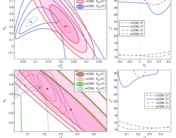
Figure 1: Contour plots of $\chi^{2}_{H}(\Omega_{m}^{0},\Omega_{k})$ with $N_{H}=57$ (the top-left panel) and with $N_{H}=31$ (the bottom-left panel) at $1\sigma$, $2\sigma$ and $3\sigma$ CL for the $\Lambda$CDM (filled contours) and $w$CDM models, the correspondent one-parameter distributions are presented in the right panels.

In the contour plots in Fig. 1 positions of $\chi^{2}_{H}$ minima are shown as the red circle and brown triangle for the $\Lambda$CDM model with, correspondingly, $N_{H}=57$ and 31; and as the blue pentagram or green hexagram for the $w$CDM model. These colors and marks will also be used below. One can see the large difference between positions of these minima points, especially for $\Omega_{m}^{0}$ with $N_{H}=57$ (observed in the top-left and bottom-right panels), the optimal values are: $\Omega_{m}^{0}\simeq 0.217$ for the $\Lambda$CDM and $\Omega_{m}^{0}\simeq 0.081$ for the $w$CDM model. The last value strongly differs from modern estimates of this parameter $\Omega_{m}^{0}\simeq 0.3$ Planck15 ; Planck18 .

In addition, if we use only the Hubble parameter $H(z)$ data, the optimal values of the curvature fraction $\Omega_{k}$ in 3 considered cases of models and $N_{H}$ are larger than $0.3$, but this value is negative for the $\Lambda$CDM with $N_{H}=31$. The positive ($\Omega_{k}>0$) $1\sigma$ domains for both models in the case $N_{H}=57$ essentially exceed the close to zero limits $\Omega_{k}=0.0007\pm 0.0037$, coming from the latest multivariate estimations Planck18 . For the case $N_{H}=31$ both model predict the best fitted values $\Omega_{k}$ with different signs (strongly separated), however these estimates do not exclude $\Omega_{k}\simeq 0$ values because of large $1\sigma$ errors (see Table 1): $\Omega_{k}=-0.13^{+0.72}_{-0.54}$ for the $\Lambda$CDM and $\Omega_{k}=0.325^{+0.367}_{-1.96}$ for the $w$CDM model with $N_{H}=31$.

On can see also the non-standard behavior of the contour plots (and the graph $\chi^{2}_{H}(\Omega_{k})$ in the bottom-left panel) in Fig. 1 for the $w$CDM model, these lines are bent. This effect appears, because at some points of the $\Omega_{m}^{0}-\Omega_{k}$ plane, when we fix $\Omega_{m}^{0}$ and $\Omega_{k}$, the function $\chi^{2}_{H}$ of two remaining parameters $H_{0}$, $w$ can have two local minima, and we should chouse the minimal one from them (coinciding with the global minimum). This “competition” between local minima is seen in Fig. 1 at points, where we “switch” from one local minimum to another during the minimization procedure in the expression (20) for $\chi^{2}_{H}(\Omega_{m}^{0},\Omega_{k})$. This effect should be carefully taken into account. Note that the $\Lambda$CDM model has no such a behavior (see Fig. 1).

For the $w$CDM model in Fig. 2 we consider (filled) contour plots for the two-parameter distribution in the $H_{0}-w$ plane: $\chi^{2}_{H}(H_{0},w)=\min\limits_{\Omega_{m}^{0},\Omega_{k}}\chi^{2}_{H}$. Here we use the same notation. However, predictions of the $\Lambda$CDM model in this plane are contracted to the $w=-1$ level line. In the right panels we show the one-parameter distributions $\chi^{2}_{H}(w)$ and $\chi^{2}_{H}(H_{0})$ (minimized over all other parameters) and the correspondent likelihood functions, in particular,

$${\cal L}_{H}(H_{0})\sim\exp(-\chi^{2}_{H}(H_{0})/2)$$ (21)

We use these functions for estimating $1\sigma$ errors, they are tabulated below in Table 1 with the best fitted values of the model parameters and minimums of $\chi^{2}_{H}$ (they are $28.82$ for the $\Lambda$CDM and $26.05$ for the $w$CDM model for $N_{H}=57$).

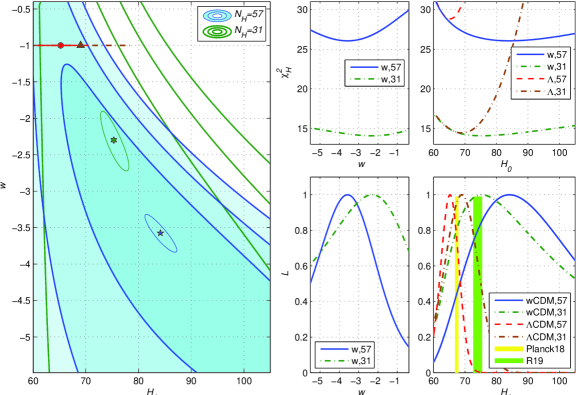
Figure 2: Contour plots of $\chi^{2}_{H}(H_{0},w)$ for the $w$CDM model with $N_{H}=57$ (filled contours) and with $N_{H}=31$ (green contours), one-parameter distributions and likelihood function ${\cal L}_{H}(w)$ and ${\cal L}_{H}(H_{0})$ are shown in the right panels. In the bottom-right panel the vertical bands refer to $H_{0}$ estimates of Planck 2018 Planck18 (yellow) and HST HST19 (green, labeled as R19).

In the bottom-right panel of Fig. 2 we draw the vertical bands describing correspondingly the $H_{0}$ estimates of Planck 2018 Planck18 and HST HST19 (labeled here and below as Planck18 and R19). These bands and $1\sigma$ estimates in different models are reproduced below in Fig. 3 in the whisker plots. One can see that for the case with $N_{H}=31$ Hubble parameter data points the $\Lambda$CDM $\chi^{2}_{H}$ prediction (the best fitted value) $H_{0}=69.0^{+5.15}_{-5.5}$ is close to Planck18 and the $w$CDM estimation $75.3^{+24.5}_{-10.8}$ corresponds to R19, so it seems (at the first glance) that we solve the $H_{0}$ tension problem, if we just switch from the $\Lambda$CDM to $w$CDM predictions under these assumptions (only $\chi^{2}_{H}$ with 31 $H(z)$ data points).

However, other optimal values of model parameters under the mentioned assumptions (see Table 1), in particular, the $w$CDM ($N_{H}=57$) estimations $\Omega_{k}=0.372^{+0.149}_{-0.13}$ are far beyond the observational limits Planck15 ; Planck18 .

Table 1: Optimal values and $1\sigma$ estimates of model parameters for $H(z)$ data

Model	Data	$N_{H}$	$\min\chi^{2}$	$H_{0}$	$\Omega_{m}^{0}$	$\Omega_{k}$	$w$
$\Lambda$CDM	$H(z)$	31	14.44	$69.0^{+5.15}_{-5.5}$	$0.360^{+0.204}_{-0.233}$	$-0.13^{+0.72}_{-0.54}$	$-1$
$w$CDM	$H(z)$	31	14.09	$75.3^{+24.5}_{-10.8}$	$0.170^{+0.425}_{-0.134}$	$0.325^{+0.367}_{-1.96}$	$-2.30^{+2.20}_{-3.22}$
$\Lambda$CDM	$H(z)$	57	28.82	$65.25^{+2.8}_{-2.9}$	$0.217^{+0.036}_{-0.040}$	$0.305^{+0.209}_{-0.18}$	$-1$
$w$CDM	$H(z)$	57	26.05	$84.2^{+21.8}_{-14.05}$	$0.081^{+0.054}_{-0.035}$	$0.372^{+0.149}_{-0.13}$	$-3.57^{+1.49}_{-1.62}$

Moreover, the best fitted $\chi^{2}_{H}$ values in the case $N_{H}=57$: $H_{0}=65.25^{+2.8}_{-2.9}$ from the $\Lambda$CDM and $84.2^{+21.8}_{-14.05}$ from the $w$CDM estimations have more larger spread than the tension between Planck18 and R19. These estimations are also illustrated in the whisker diagram in Fig. 3, corresponding the bottom-right panel of Fig. 2 in comparison with the results, determined by the function $\chi^{2}_{H+\mbox{\scriptsize SN}}$.

Figure 3: Whisker plots for $\chi^{2}_{H}$, $\chi^{2}_{H+\mbox{\scriptsize SN}}$ and 2 models with different $N_{H}$ in comparison with Planck18 and R19 $H_{0}$ estimates.

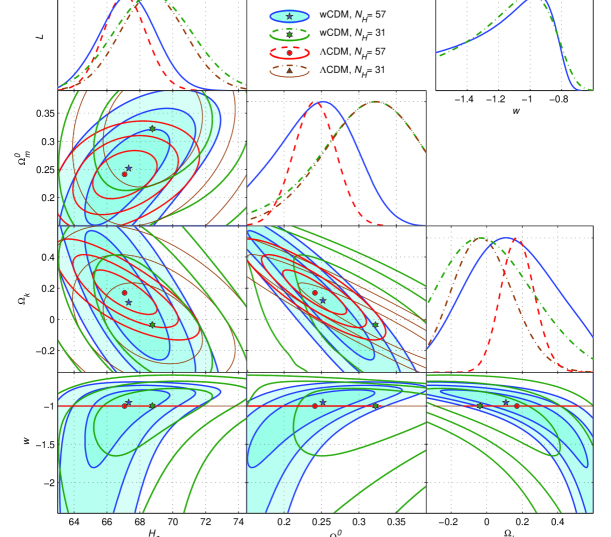
Figure 4: Contour plots and one-parameter distributions of $\chi^{2}_{H+\mbox{\scriptsize SN}}$ ($H(z)$ and the Pantheon SNe Ia data) for the $\Lambda$CDM and $w$CDM models.

Keeping in mind the non-standard estimations of $H_{0}$, $\Omega_{k}$ and behavior in the $\Omega_{m}^{0}-\Omega_{k}$ and $H_{0}-w$ planes, one may conclude, that the Hubble parameter observations $H(z)$ alone do not give an adequate picture of the $\Lambda$CDM and $w$CDM cosmology during $0\leq z\leq 2.36$. Hence, we should add other observational data described above in Sect. III, in particular, SNe Ia data Scolnic17 .

We consider further the $H(z)$ with SNe Ia data set described by the function $\chi^{2}_{H+\mbox{\scriptsize SN}}=\chi^{2}_{H}+\chi^{2}_{\mbox{\scriptsize SN}}$ (16): the results are depicted in Fig. 4, where we compare the $\Lambda$CDM and $w$CDM models in 6 planes with contour plots ($H_{0}-\Omega_{m}^{0}$, $H_{0}-\Omega_{k}$, $\Omega_{m}^{0}-\Omega_{k}$, $\Omega_{m}^{0}-\Omega_{k}$, etc.) and in 4 panels with one-parameter likelihood functions ${\cal L}_{H+\mbox{\scriptsize SN}}(p_{j})$ of the type (21). In all panels the blue filled contours and blue lines correspond to $\chi^{2}_{H+\mbox{\scriptsize SN}}$ for the $w$CDM model with $N_{H}=57$, colors and labels of minima points for other variants are the same as in Figs. 1 and 2.

The one-parameter likelihood functions ${\cal L}_{H+\mbox{\scriptsize SN}}$ in Fig. 4 let us calculate the best fitted values and corresponding error bands presented in Table 2.

One may observe in Fig. 4 that the Pantheon SNe Ia data, included in our analysis, significantly change the best fitted values for all parameters and all variants of the models (supporting the above mentioned irrelevance of only Hubble parameter data). These values for $\chi^{2}_{H+\mbox{\scriptsize SN}}$ are tabulated in Table 2. In particular, the exotic $\chi^{2}_{H}$ estimates for the $w$CDM ($N_{H}=57$) model $\Omega_{m}^{0}=0.081^{+0.054}_{-0.035}$, $w=-3.57^{+1.49}_{-1.62}$ in the case $\chi^{2}_{H+\mbox{\scriptsize SN}}$ return to their “normal” values (corresponding to recent estimates Planck15 ; Planck15 ): $\Omega_{m}^{0}=0.252^{+0.048}_{-0.061}$, $w=-0.954^{+0.124}_{-0.33}$. The similar changes (up to $\Omega_{m}^{0}=0.322^{+0.066}_{-0.069}$) take place also for the $w$CDM model with $N_{H}=31$; in this case the optimal $w$CDM value $w=-0.988^{+0.166}_{-0.32}$ appears to be extremely close the $\Lambda$CDM limit $w=-1$ and the best fitted estimates of all parameters practically coincide for these two models.

Fig. 4 also demonstrates the large difference between the $\Omega_{m}^{0}$ estimates for the cases $N_{H}=31$ and 57. The similar difference may be seen for the Hubble parameter $H_{0}$, however the whisker plot in Fig. 3 shows, that it is essentially less than for the only $\chi^{2}_{H}$ data. Thus, one may conclude, that for the Hubble parameter plus SNe Ia data ($\chi^{2}_{H+\mbox{\scriptsize SN}}$) in all 4 considered variants of the $\Lambda$CDM and $w$CDM models only Planck18 estimates of $H_{0}$ are supported: all models are in tension with the HST (R19) data.

V Additional analysis of CMB data

In this section we add the cosmic microwave background radiation (CMB) data in the form $\chi^{2}_{\mbox{\scriptsize CMB}}$ (18), (19) HuangWW2015 to the previous $H(z)$ and SNe Ia data sets and analyze the resulting $\chi^{2}$ function

$$\chi^{2}_{\mbox{\scriptsize tot}}=\chi^{2}_{H}+\chi^{2}_{\mbox{\scriptsize SN}}+\chi^{2}_{\mbox{\scriptsize CMB}}.$$ (22)

The results of $\chi^{2}_{\mbox{\scriptsize tot}}$-based calculations are presented in Fig. 5 and in Table 2.

One can expect from the previous papers OdintsovSGS2017 ; OdintsovSGS2019 (and will see in Fig. 5) that the included CMB data strongly change estimations for model parameters and especially for their error boxes. In particular, calculated from $\chi^{2}_{\mbox{\scriptsize tot}}$ error boxes for $\Omega_{m}^{0}$ are essentially more narrow because of small errors $\sigma_{i}$ in the CMB priors (19) of the values (17) with the parameter $R$ proportional to $\sqrt{\Omega_{m}^{0}}$.

Figure 5: Contour plots and one-parameter distributions of $\chi^{2}_{\mbox{\scriptsize tot}}$ ($H+{}$SNe Ia${}+{}$CMB data) for the $\Lambda$CDM and $w$CDM models.

In Fig. 5 and in Table 2 we can observe, that the predicted from $\chi^{2}_{\mbox{\scriptsize tot}}$ ($H+{}$SNe Ia${}+{}$CMB) error bands are strongly contracted (in comparison with $\chi^{2}_{H+\mbox{\scriptsize SN}}$) not only for $\Omega_{m}^{0}$ (where the error box is of order $\Delta\Omega_{m}^{0}\simeq 0.0017$), but also for $\Omega_{k}$, where $\Delta\Omega_{k}\simeq 0.0017$ for the $\Lambda$CDM and $\Delta\Omega_{k}\simeq 0.004$ for the $w$CDM model. One should note also, that the best fitted estimates of $\Omega_{m}^{0}$ with the CMB data are rather close in the range $0.282<\Omega_{m}^{0}<0.283$ for all 4 considered variants. For $\Omega_{k}$ the optimal values lie in the range $0.0055\leq\Omega_{k}\leq 0.011$ and slightly differ for the $\Lambda$CDM and $w$CDM models.

However, for the Hubble constant the influence of the CMB data is not so striking: the $H_{0}$ error bands for $\chi^{2}_{\mbox{\scriptsize tot}}$ appear to be about $1.5$ times diminished in comparison with the case.

Estimations of the Hubble constant $H_{0}$ (shown in the top-left panel of Fig. 5) and the correspondent whisker plot with $1\sigma$ error boxes are presented in Fig. 6. Here we also compare the results for $H+{}$SNe Ia${}+{}$CMB data with the previous estimates from the function $\chi^{2}_{H+\mbox{\scriptsize SN}}$. One can note that the included CMB data almost do not change the best fitted $H_{0}$ estimates (with the mentioned contraction of their error boxes) for the $w$CDM model, but the $H_{0}$ estimates, but the $H_{0}$ estimates for the $\Lambda$CDM model appear to be enlarged. However, this growth is too small for describing the HST (R19) estimations, that could be a solution of the $H_{0}$ tension problem.

The most successful variant for solving this problem is to consider the flat case ($k=0$) of the $\Lambda$CDM or $w$CDM models. This variant is the particular case of these models, if we just suppose $\Omega_{k}=0$ in our calculations. The corresponding result $H_{0}=70.87^{+1.63}_{-1.62}$ km /(s$\cdot$Mpc) for the flat $w$CDM model with $N_{H}=31$ is shown in Fig. 6 with black color. The $1\sigma$ band for this variant is very close to R19 estimates, however only the correspondent $2\sigma$ band (shown as the dashed line) reaches the R19 range.

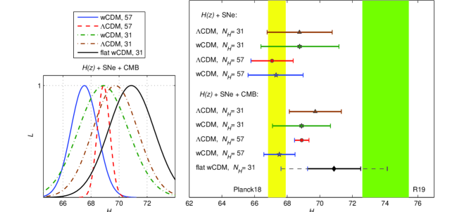
Figure 6: Likelihoods for $\chi^{2}_{\mbox{\scriptsize tot}}$ ($H+{}$SNe Ia${}+{}$CMB) with the correspondent whisker plot (with the previous case $\chi^{2}_{H+\mbox{\scriptsize SN}}$) in comparison with Planck18 and R19 $H_{0}$ estimates. The dashed line describes the $2\sigma$ error band, solid thick lines correspond to $1\sigma$ estimates.

VI Conclusion

In this paper we considered two cosmological models $\Lambda$CDM and $w$CDM in confrontation with different observational data: the Hubble parameter $H(z)$ estimations (31 data points from cosmic chronometers and the extended sample with 57 data points), the Pantheon sample Type Ia supernovae data Scolnic17 and CMB data in the form (18), (19) HuangWW2015 . In this study we, in particular, kept in mind a possibility to alleviate the Hubble constant tension between the Planck Planck13 ; Planck15 ; Planck18 and HST HST18 ; HST19 estimations of $H_{0}$.

We have shown that the $H_{0}$ tension can be easily explained (with simple “switching” from the $\Lambda$CDM to $w$CDM model), if we consider only the $H(z)$ data via the $\chi^{2}_{H}$ function (13) (see Figs. 2, 3). However, this approach with the extremely poor set of observations is not acceptable, because it predicts extraordinary values of model parameters in Table 1.

The model predictions become reliable, when we include into consideration the SNe Ia Scolnic17 and CMB data HuangWW2015 . The resulting best fitted values of model parameters with $1\sigma$ errors for the $\chi^{2}$ functions $\chi^{2}_{H+\mbox{\scriptsize SN}}$ (16) and $\chi^{2}_{\mbox{\scriptsize tot}}=\chi^{2}_{H+\mbox{\scriptsize SN}}+\chi^{2}_{\mbox{\scriptsize CMB}}$ (22) are presented in Table 2. The corresponding results for Hubble constant $H_{0}$ are shown in Fig. 6, they essentially depend on chosen filters inside the models (for example, if we fix $w=-1$ or $\Omega_{k}=0$) or filters applied to observations.

Table 2: The best fitted values and $1\sigma$ estimates of model parameters for $H(z)+{}$SN and CMB data

Model	Data	$N_{H}$	$\min\chi^{2}$	$H_{0}$	$\Omega_{m}^{0}$	$\Omega_{k}$	$w$
$\Lambda$CDM	$H$+SN	$31$	$1072.76$	$68.75^{+2.01}_{-1.98}$	$0.322^{+0.066}_{-0.068}$	$-0.035^{+0.176}_{-0.167}$	$-1$
$w$CDM	$H$+SN	$31$	$1072.76$	$68.76^{+2.41}_{-2.37}$	$0.322^{+0.066}_{-0.069}$	$-0.036^{+0.290}_{-0.258}$	$-0.988^{+0.166}_{-0.32}$
$\Lambda$CDM	$H$+SN	$57$	$1088.76$	$67.07^{+1.30}_{-1.29}$	$0.242^{+0.027}_{-0.029}$	$0.170^{+0.096}_{-0.092}$	$-1$
$w$CDM	$H$+SN	$57$	$1088.70$	$67.32^{+1.66}_{-1.72}$	$0.252^{+0.048}_{-0.061}$	$0.108^{+0.30}_{-0.251}$	$-0.954^{+0.124}_{-0.330}$
$\Lambda$CDM	$H$+SN+CMB	$31$	$1074.29$	$69.72^{+1.60}_{-1.59}$	$0.2829^{+0.0017}_{-0.0018}$	$0.0056^{+0.0017}_{-0.0017}$	$-1$
$w$CDM	$H$+SN+CMB	$31$	$1073.20$	$68.88^{+1.77}_{-1.78}$	$0.2826^{+0.0017}_{-0.0018}$	$0.009^{+0.004}_{-0.004}$	$-0.945^{+0.051}_{-0.053}$
$\Lambda$CDM	$H$+SN+CMB	$57$	$1092.09$	$68.89^{+0.45}_{-0.44}$	$0.2426^{+0.0017}_{-0.0017}$	$0.0055^{+0.0017}_{-0.0017}$	$-1$
$w$CDM	$H$+SN+CMB	$57$	$1089.44$	$67.52^{+0.96}_{-0.95}$	$0.2822^{+0.0017}_{-0.0018}$	$0.011^{+0.004}_{-0.004}$	$\!-0.922^{+0.048}_{-0.048}\!$

If we concentrate on the $H_{0}$ tension problem, we may conclude that the most successful scenario for its alleviation is the $w$CDM model with the maximal data set (for $\chi^{2}_{\mbox{\scriptsize tot}}=\chi^{2}_{H+\mbox{\scriptsize SN}+\mbox{\scriptsize CMB}}$): the best fitted value $H_{0}=67.52^{+0.96}_{-0.95}$ km s^-1Mpc^-1 for $N_{H}=57$ almost coincides with the Planck 18 estimate Planck18 ; from the other side, if we accept the flat variant of this model (fix $\Omega_{k}=0$) we obtain $H_{0}=70.87^{+1.63}_{-1.62}$ km s^-1Mpc^-1 for $N_{H}=31$ that is very close to the HST estimation HST19 (the green band in Fig. 6), but it is not large enough and lies outside the $1\sigma$ confidence level (only $2\sigma$ bands have intersection).

One may conclude that the $w$CDM model has considerable achievements, but it is not successful enough for conclusive solving the $H_{0}$ tension problem on the base of the mentioned observational data. For this purpose we should investigate some its extensions or other cosmological scenarios DiValentMLS2017  – DiValentMMVw2019 .

References

- (1) Ade P.A.R. et al. Planck 2013 results. XVI. Cosmological parameters. Astron. Astrophys. 2014, 571, A16, 66pp. (arXiv: 1303.5076)
- (2) Planck Collaboration, Ade P.A.R. et al. Planck 2015 results. XIII. Cosmological parameters. Astron. Astrophys. 2016, 594, A13, 66pp. (arXiv: 1502.01589)
- (3) Planck Collaboration, Aghanim N. et al. Planck 2018 results. VI. Cosmological parameters. (arXiv: 1807.06209)
- (4) Riess A.G. et al. Milky Way Cepheid Standards for Measuring Cosmic Distances and Application to Gaia DR2: Implications for the Hubble Constant. Astrophys J. 2018, 861, 126, 13 pp. (arXiv: 1804.10655)
- (5) Riess A.G. , Casertano S., Yuan W., Macri L.M. and Scolnic D. Large Magellanic Cloud Cepheid Standards Provide a 1% Foundation for the Determination of the Hubble Constant and Stronger Evidence for Physics Beyond LambdaCDM. Astrophys J. 2019, 876, 85, 13 pp. (arXiv: 1903.07603)
- (6) Huang Q.-G. and Wang K. How the dark energy can reconcile Planck with local determination of the Hubble Constant. Eur. Phys. J. 2016, C76, 506, 5 pp. (arXiv: 1606.05965)
- (7) Zhao M.-M., He D.-Z., Zhang J.-F. and Zhang X. Search for sterile neutrinos in holographic dark energy cosmology: Reconciling Planck observation with the local measurement of the Hubble constant. Phys. Rev. 2017, D96, 043520, 9 pp. (arXiv: 1703.08456)
- (8) Di Valentino E., Melchiorri A., Linder E. V. and Silk J. Constraining Dark Energy Dynamics in Extended Parameter Space. Phys. Rev. 2017, D96, 023523, 10 pp. (arXiv: 1704.00762)
- (9) Yang W., Pan S. and Paliathanasis A. Latest astronomical constraints on some non-linear parametric dark energy models. Mon. Not. Roy. Astron. Soc. 2018, 475, 2605 2613, 9 pp. (arXiv: 1708.01717)
- (10) Di Valentino E., Linder E. V. and Melchiorri A. A Vacuum phase transition solves the tension. Phys. Rev. 2018, D97, 043528, 12 pp. (arXiv: 1710.02153)
- (11) Di Valentino E., Bøehm C., Hivon E. and Bouchet F. R. Reducing the and tensions with Dark Matter-neutrino interactions. Phys. Rev. 2018, D97, 043513, 13 pp. (arXiv: 1710.02559)
- (12) Khosravi N., Baghram S., Afshordi N. and Altamirano N. tension as a hint for a transition in gravitational theory. Phys. Rev. 2019, D99, 103526, 11 pp. (arXiv: 1710.09366)
- (13) Benetti M., Graef L. L. and Alcaniz J. S. The and tensions and the scale invariant spectrum. JCAP 2018, 1807, 066, 4 pp. (arXiv: 1712.00677)
- (14) Mörtsell E. and Dhawan S. Does the Hubble constant tension call for new physics? JCAP 2018, 1809, 025, 24 pp. (arXiv: 1801.07260)
- (15) Nunes R. C. Structure formation in f(T) gravity and a solution for tension. JCAP 2018, 1805, 052, 17 pp. (arXiv: 1802.02281)
- (16) Guo R.-Y., Zhang J.-F. and Zhang X. Can the tension be resolved in extensions to CDM cosmology? JCAP 2019, 1902, 054, 10 pp. (arXiv: 1809.02340)
- (17) Yang W., Pan S., Di Valentino E., Saridakis E. N. and Chakraborty S. Observational constraints on one-parameter dynamical dark-energy parametrizations and the tension. Phys. Rev. 2019, D99, 043543, 14 pp. (arXiv: 1810.05141)
- (18) Poulin V., Smith T. L., Karwal T. and Kamionkowski M. Early Dark Energy Can Resolve The Hubble Tension. Phys. Rev. Lett. 2019, 122, 221301, 7 pp. (arXiv: 1811.04083)
- (19) Pandey K. L., Karwal T. and Das S. Alleviating the and anomalies with a decaying dark matter model. 2019, 18 pp. (arXiv: 1902.10636)
- (20) Vagnozzi S. New physics in light of the tension: an alternative view. 2019, 23 pp. (arXiv: 1907.07569)
- (21) Di Valentino E., Melchiorri A. and Mena O. Can interacting dark energy solve the tension? Phys. Rev. 2017, D96, 043503, 11 pp. (arXiv: 1704.08342)
- (22) Yang W., Pan S., Di Valentino E., Nunes R. C., Vagnozzi S. and Mota D. F. Tale of stable interacting dark energy, observational signatures, and the tension. JCAP 2018, 1809, 019, 21 pp. (arXiv: 1805.08252)
- (23) Yang W., Mukherjee A., Di Valentino E. and Pan S. Interacting dark energy with time varying equation of state and the tension Phys. Rev. 2018, D98, 123527, 15 pp. (arXiv: 1809.06883)
- (24) Kumar S., Nunes R. C. and Yadav S. K. Dark sector interaction: a remedy of the tensions between CMB and LSS data. Eur. Phys. J. 2019, C79, 576, 5 pp. (arXiv: 1903.04865)
- (25) Pan S., Yang W., Singha C. and Saridakis E. N. Observational constraints on sign-changeable interaction models and alleviation of the tension. Phys. Rev. 2019, D100, 083539, 20 pp. (arXiv: 1903.10969)
- (26) Pan S., Yang W., Di Valentino E., Saridakis E. N. and Chakraborty S. Interacting scenarios with dynamical dark energy: observational constraints and alleviation of the H0 tension. Phys. Rev. 2019, D100, 103520, 19 pp. (arXiv: 1907.07540)
- (27) Di Valentino E., Melchiorri A., Mena O. and Vagnozzi S. Interacting dark energy after the latest Planck, DES, and measurements: an excellent solution to the and cosmic shear tensions. (arXiv: 1908.04281)
- (28) Di Valentino E., Melchiorri A., Mena O. and Vagnozzi S. Non-minimal dark sector physics and cosmological tensions. (arXiv: 1910.09853)
- (29) Mota D.F. and Barrow J.D. Local and Global Variations of The Fine Structure Constant. Mon. Not. Roy. Astron. Soc. 2004, 349, pp. 291?302 (arXiv: astro-ph/0309273)
- (30) Brevik I., Nojiri S., Odintsov S.D. and Vanzo L. Inhomogeneous Equation of State of the Universe: Phantom Era, Future Singularity and Crossing the Phantom Barrier Phys. Rev. D. 2004, 70, 043520, 19 pp. (arXiv: hep-th/0401073)
- (31) Nojiri S. and Odintsov S.D. Entropy and universality of Cardy-Verlinde formula in dark energy universe Phys. Rev. D. 2005, 72, 023003, 13 pp. (arXiv: hep-th/0505215)
- (32) Grigorieva O.A. and Sharov G.S. Multidimensional gravitational model with anisotropic pressure. Intern. Journal of Modern Physics D 2013, 22, 1350075 (arXiv: 1211.4992)
- (33) Sharov G.S. and Vorontsova E.G. Parameters of cosmological models and recent astronomical observations. J. Cosmol. Astropart. Phys. 2014, 10, 057, 21pp. (arXiv: 1407.5405)
- (34) Sharov G.S. Observational constraints on cosmological models with Chaplygin gas and quadratic equation of state. J. Cosmol. Astropart. Phys. 2016, 06 023, 24pp. (arXiv: 1506.05246)
- (35) Sharov G.S., Bhattacharya S., Pan S., Nunes R.C. and Chakraborty S. A new interacting two fluid model and its consequences. Mon. Not. Roy. Astron. Soc. 2017, 466, 3497pp. (arXiv: 1701.00780)
- (36) Pan S. and Sharov G.S. A model with interaction of dark components and recent observational data. Mon. Not. Roy. Astron. Soc. 2017, 472, 4736pp. (arXiv: 1609.02287)
- (37) Odintsov S.D., Saez-Gomez D. and Sharov G.S. Is exponential gravity a viable description for the whole cosmological history? European Phys. J. C. 2017, 77, 862, 17pp. (arXiv: 1709.06800)
- (38) Sharov G.S. and Vasiliev V.O. How predictions of cosmological models depend on Hubble parameter data sets. Math. Modelling and Geometry. 2018 V. 6, No 1, P. 1: arXiv:1807.07323; doi:10.26456/mmg/2018-611 (arXiv: 1012.2280)
- (39) Sharov G.S. and Vorontsova E.G. Cosmological models with integrable equations of state (in Russian). Vestnik TVGU. Ser. Prikl. Matem. [Herald of Tver State University. Ser. Appl. Math.], 2018, Issue 2, Pp. 5 26; https://doi.org/10.26456/vtpmk192
- (40) Odintsov S.D., Saez-Gomez D. and Sharov G.S. Testing logarithmic corrections on -exponential gravity by observational data Phys. Rev. D. 2019, 99, 024003, 17 pp. (arXiv: 1807.02163)
- (41) Scolnic D.M. et al., The Complete Light-curve Sample of Spectroscopically Confirmed Type Ia Supernovae from Pan-STARRS1 and Cosmological Constraints from The Combined Pantheon Sample Astrophys. J. 2018, 859, 101, 28pp. (arXiv: 1710.00845)
- (42) Huang Q.-G., Wang K. and Wang S. Distance Priors from Planck 2015 data. J. Cosmol. Astropart. Phys. 2015, 1512, 022, 18pp. (arXiv: 1509.00969)
- (43) Nojiri S. and Odintsov S.D. Unified cosmic history in modified gravity: from F(R) theory to Lorentz non-invariant models. Physics Reports 2011, 505, pp. 59 – 144 (arXiv: 1011.0544)
- (44) Bamba K., Capozziello S., Nojiri S. and Odintsov S.D. Dark energy cosmology: the equivalent description via different theoretical models and cosmography tests. Astrophys. and Space Science 2012, 342, pp. 155 – 228 (arXiv: 1205.3421)
- (45) Kirshner R.P. Foundations of supernova cosmology. In Dark Energy – Observational and Theoretical Approaches. Ed. Pilar Ruiz-Lapuente. 2010, 151pp. New York by Cambridge University Press (arXiv: 0910.0257)
- (46) Suzuki N. et al. The Hubble Space Telescope Cluster Supernova Survey: V. Improving the Dark Energy Constraints Above and Building an Early-Type-Hosted Supernova Sample. Astrophys. J. 2012, 746, 85, 24pp. (arXiv: 1105.3470)