Representation Learning on Variable Length and Incomplete Wearable-Sensory Time Series

Abstract.

The prevalence of wearable sensors (e.g., smart wristband) is creating unprecedented opportunities to not only inform health and wellness states of individuals, but also assess and infer personal attributes, including demographic and personality attributes. However, the data captured from wearables, such as heart rate or number of steps, present two key challenges: 1) the time series is often of variable-length and incomplete due to different data collection periods (e.g., wearing behavior varies by person); and 2) inter-individual variability to external factors like stress and environment. This paper addresses these challenges and brings us closer to the potential of personalized insights about an individual, taking the leap from quantified self to qualified self. Specifically, HeartSpace proposed in this paper encodes time series data with variable-length and missing values via the integration of a time series encoding module and a pattern aggregation network. Additionally, HeartSpace implements a Siamese-triplet network to optimize representations by jointly capturing intra- and inter-series correlations during the embedding learning process. The empirical evaluation over two different real-world data presents significant performance gains over state-of-the-art baselines in a variety of applications, including personality prediction, demographics inference, and user identification.

1. Introduction

The wide proliferation of wearables and mobile devices is revolutionizing health and wellness with the potential of data and personalized insights at one’s fingertips  (Op De Beéck, Meert, and others, 2018). These wearables generate chronologically ordered streams (e.g., the series of heart rate measurements) or point-in-time activity (e.g., the number of steps) or general summarization of the day (e.g., move goals). Collectively, these data provide an insight abut quantified self, and are also providing an unprecedented opportunity to infer qualitative attributes about an individual, including demographics, social network, opinions, beliefs, personality, and job performance.

In this paper, we pose the problem of inferring personal attributes about an individual (qualified self) from the quantified data generated from wearables. Specifically, we focus on the challenges presented from the chronologically ordered data generated from the wearables (such as the heart rate data). This data is notated as wearable-sensory time series in this paper. We posit that it is critical to effectively model these these wearable-sensory time series data to fully realize their benefit for a wide spectrum of applications, such as personality detection (Cao et al., 2017), job performance prediction, health and wellness state assessment and prediction, user identification (Wang et al., 2018b) and demographics inference (Wang et al., 2016).

However, wearable-sensory time series data present a number of challenges, including temporal dependencies, incompleteness, intra-sensor / individual variability, and inter-individual variability. In this paper, we address these challenges by developing a generalized representation learning algorithm, HeartSpace, and demonstrate how physiological responses as captured in the heart rate is predictive and indicative of several personal attributes, including demographics and personality.

Limitations of Current Work.

The contemporary body research in time series has focused on wavelet-based frequency analysis (Sun, Leng, and etc, 2015) and / or motif discovery methods (Zhu et al., 2018). First, while we can extract discriminating and independent features using wavelet decomposition approaches, it still involves manual effort and domain-specific expert knowledge (e.g., medical knowledge) (Bai et al., 2018). Second, discovering motifs are computationally expensive and require the repeated process of searching for optimal motifs from candidates (Liu et al., 2015).

Motivated by these limitations, recent research has also focused on representation learning on sensory data (Ballinger et al., 2018; Wang et al., 2018a; Ni, Muhlstein, and McAuley, 2019). But these works are also limited as they assume complete time series and fixed length sequences, thus not sufficiently addressing the following challenges. First, the wearable-sensory time series data is of variable-length ranging from several days to months, since the active sensing time period may vary from person to person (Liu et al., 2016). Second, readings of sensors are usually missing / incomplete at different time periods for various reasons (e.g., sensor communication errors or power outages or compliance) (Manashty, Light, and Soleimani, 2018). Third, the success of these supervised deep neural network models largely relies on substantial ground truth (Choi, Bahadori, and others, 2017), which is often scarce.

This paper.

In light of these challenges and limitations, we developed a time series representation learning model, HeartSpace, that addresses the weaknesses of the aforementioned methods and learns generalized embeddings, leading to more accurate models to infer and predict user demographics, personality, work performance attributes, and health states. Specifically, HeartSpace addresses the following key challenges:
1) Handling variable-length time series and data incompleteness. A straightforward way to address variable-length input is to resize each input time series into a fixed-length vector. However, the resulting vector, derived by interpolation when input length differs from pre-defined length, has less control of variable time series resolutions and fails to capture the consistent time granularity for different individuals, leading to inferior representation. An alternative approach is sequence padding with specific symbols so that all time series are as long as the longest series in the dataset (Srivastava, Greff, and Schmidhuber, 2015). However, an associated challenge with sequence padding is that all time series data have been artificially created with fixed-length inefficiently (Doetsch, Golik, and Ney, 2017). Consequently, artificially created sequences with padding operation may not properly reflect their time-evolving distributions. This is especially critical when trying to draw insights from physiological response data such as heart rate. Thus, a representation learning method should be able to deal with variable length and incomplete data.
2) Differentiating unique patterns from time series data with similar trends. In addition, the wearable-sensory data collected from different people may have very similar distributions (Yang, Dumont, and etc, 2006). For example, for adults 18 and older, a normal resting heart rate (i.e.number of heart beats per minute) is between 60 and 80 beats per minute (Ballinger et al., 2018). However, there are localized patterns among individuals (intra-sensor / individual variability) that offer important nuances on similarities and differences. Thus, a representation learning method should be able to capture the global and local characteristics of such time series data to effectively compute similarities among individuals. To summarize, our main contributions are as follows.

We develop a novel and effective representation learning model, HeartSpace, that successfully addresses the aforementioned challenges to learn a generalizable lower-dimensional and latent embedding from wearable sensory data. In HeartSpace, we first segment the heart rate data collected from individuals into multiple day-long time series because human behavior to capture day-long regularities. Then, a deep autoencoder architecture is developed to map high-dimensional time-specific (i.e., daily) sensor data into the same latent space with a dual-stage gating mechanism. These learned embedding vectors are capable of not only preserving temporal variation patterns, but also largely alleviating the data missing issue of wearable-sensory time series. After that, we leverage a temporal pattern aggregation network to capture inter-dependencies across time-specific representations based on the developed position-aware multi-head attention mechanism. During the training process, a Siamese-triplet network optimization strategy is designed with the exploration of implicit intra-series temporal consistency and inter-series relations. We evaluate HeartSpace on two real-world wearable-sensory time series data representing a diverse group of human subjects and two different sensing devices. Our experiments demonstrate that HeartSpace outperforms the state-of-the-art methods in various applications, including user identification, personality prediction, demographics inference, and job performance prediction, thereby asserting the quality of the learned embedding. To the best of our knowledge, this is the most comprehensive study on addressing challenges of wearable time series data by developing a novel HeartSpace, considering two real-world data representative of different human subjects and environments, and applying to a number of application scenarios.

2. Problem Formulation

We first introduce preliminary definitions and formalize the problem of wearable-sensory time series representation learning. We use bold capital and bold lower case letters to denote matrices and vectors, respectively.

Definition 1.

Wearable-Sensory Time Series. Suppose there are $I$ users ($U=\{u_{1},...,u_{i},...,u_{I}\}$), and $\textbf{X}_{i}=(x_{i}^{1},...,x_{i}^{j},...,x_{i}^{J_{i}})$ ($\textbf{X}_{i}\in\mathbb{R}^{J_{i}}$) to denote the series of temporally ordered wearable-sensory data (e.g., heart rate measurement — the number of times a person’s heart beats per minute) of length $J_{i}$ collected from user $u_{i}$. In particular, each element $x_{i}^{j}$ represents the $j$-th measured quantitative value from user $u_{i}$ ($1\leq j\leq J_{i}$ and $J_{i}$ may vary from user to user. Each measurement $x_{i}^{j}$ is associated with a timestamp information $t_{i}^{j}$ and thus we define a time vector $\textbf{T}_{i}=(t_{i}^{1},...,t_{i}^{j},...,t_{i}^{J_{i}})$ to record the timestamp information of sequential wearable sensor data $\textbf{X}_{i}$.

Since the wearable-sensory data is collected over different time periods (e.g., with different start and end date), the sequence lengths usually vary among different time series (Liu et al., 2016). Additionally, readings of wearable sensors are usually lost at various unexpected moments because of sensor or communication errors (e.g., power outages) (Manashty, Light, and Soleimani, 2018). Therefore, the wearable-sensory data often exhibit variable-length and missing values.

Problem Statement. Wearable-Sensory Time Series Representation Learning. Given a wearable-sensory time series $\textbf{X}_{i}$ with variable-length and missing values, the objective is to learn the $d$-dimensional latent vector $\textbf{Y}_{i}\in\mathbb{R}^{d}$ that is able to capture the unique temporal patterns of time series $\textbf{X}_{i}$.

The output of the model is a low-dimensional vector $\textbf{Y}_{i}$ corresponding to the latent representation of each wearable-sensory time series $\textbf{X}_{i}$ from user $u_{i}$. Notice that, although different time series $\textbf{X}_{i}(i\in[1,...,I])$ can be of any length, their representations are mapped into the same latent space. This learned time series representations, generated by HeartSpacecan benefit various health and wellness tasks without the requirement of substantial training instance pairs.

3. Methodology: HeartSpace

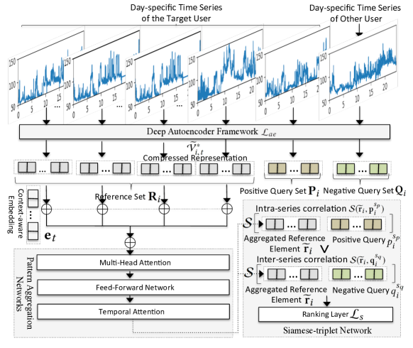
Figure 1. HeartSpace Framework. The training flow can be summarized as: (1) partition raw sensory data to a set of day-long time series; (2) map each day-long time series into a representation vector by Day-Specific Time Series Encoding Module (3) fuse day specific representations through Temporal Pattern Aggregation Network (4) update parameters based on reconstruction loss and Siamese-triple loss.

Time Series Segmentation

Considering that periodicity has been demonstrated as an important factor that governs human sensory data (e.g., heart rate) with time-dependent transition regularities (Nakamura, Takimoto-Inose, and etc, 2018), and the sensed time series data are often variable-length, we first partition the wearable-sensory time series (i.e., $\textbf{x}_{i}$) of each user $u_{i}$ into $T$ (indexed by $t$) separated day-long time series ($T$ may vary among users).

Definition 2.

Day-long Time Series $\mathbf{x}_{i,t}$. Each $t$-th divided day-long time series of $\textbf{x}_{i}$ is denoted as $\textbf{x}_{i,t}\in\mathbb{R}^{K}$, where $K=1440$ is the number of minutes included in one day. In $\textbf{x}_{i,t}$, each element $x_{i,t}^{k}$ is the measurement from user $u_{i}$ at the $k$-th time step in $\textbf{x}_{i,t}$. Due to the data incompleteness issue of the collected time series, we set the element $x_{i,t}^{k}$ as 0 to keep equally-spaced intervals for missing measurement.

Leveraging the Day-long Time Series, HeartSpace consists of three components: i) Day-specific time series encoding; ii) Temporal pattern aggregation network; and iii) Siamese-triplet network optimization strategy.

3.1. Day-Specific Time Series Encoding

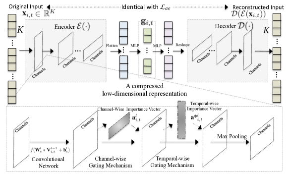
Figure 2. Illustration of Day-Specific Time Series Encoding.

To explore the underlying repeated local patterns and reduce dimensions of day-long time series data, we first propose a convolution autoencoder module to map each individual series $\textbf{x}_{i,t}$ into a common low-dimensional latent space. In general, the encoder first takes day-long time series as the input and then translates it into a latent representation which encodes the temporal pattern. Then, the decoder network reconstructs the data which is identical with the input $\textbf{x}_{i,t}$ in the ideal case. To keep the input dimension consistent with complete day-specific time series, we impute missing values with zero, as typically done. Since the imputed values are treated same as other valid inputs when applying kernels in each convolutional layer, the generated features can get incorrectly encoded and further lead to error propagation from lower to higher layers. To resolve this issue stemming from zero padding, we propose a dual-stage gating mechanism into the convolution autoencoder module. More specifically, each layer of our deep autoencoder framework is a four-step block: i) convolution network; ii) channel-wise gating mechanism; iii) temporal gating mechanism; and iv) pooling operation. Figure 2 presents the architecture of our deep autonencoder module.

3.1.1. Convolutional Layers

Firstly, we apply convolutional layers to encode the local pattern of day-long time series $\textbf{x}_{i,t}$. Let’s denote $\mathbf{V}_{i,t}^{l-1}$as the feature map representation of $(l-1)$-th layer. The output of $l$-th layer is given as:

(1) $$\small\mathbf{V}_{i,t}^{l}=f(\textbf{W}^{l}_{c}*\mathbf{V}_{i,t}^{l-1}+\textbf{b}^{l}_{c})$$

where $f(\cdot)$ is the activation function and $*$ denotes the convolutional operation. $\textbf{W}^{l}_{c}$ and $\textbf{b}^{l}_{c}$ represents the transformation matrix and bias term in $l$-th layer, respectively.

3.1.2. Channel-Wise Gating Mechanism

The goal of the channel-wise gating mechanism is to re-weight hidden units by exploiting the cross-channel dependencies and selecting the most informative elements from the encoded feature representation $\mathbf{V}_{i,t}^{l}$ (Hu, Shen, and Sun, 2018). To exploit the dependencies over channel dimension, we first apply temporal average pooling operation $\mathcal{F}_{pool}^{cg}(\cdot)$ on the feature representation $\mathbf{V}_{i,t}^{l}$ over temporal dimension ($1\!\!\leq\!\!k\!\!\leq\!\!K$) to produce the summary of each channel-wise representation as:

(2) $$\small\textbf{z}_{i,t}^{l}=\mathcal{F}_{pool}^{cg}(\mathbf{V}_{i,t}^{l})=\frac{1}{K}\sum_{k=1}^{K}\mathbf{V}_{i,t,k,:}^{l}$$

where $\textbf{z}_{i,t}^{l}$ is the intermediate representation of $\mathbf{V}_{i,t}^{l}$ after average pooling operation over temporal dimension. Then, our channel-wise gating mechanism recalibrates the information distribution among all elements across channels as:

(3) $$\small\textbf{a}_{i,t}^{l}=\text{Sigmoid}(\textbf{W}_{2}^{cg}\cdot\text{ReLU}(\textbf{W}_{1}^{cg}\cdot\textbf{z}_{i,t}^{l}))$$

where $\textbf{a}_{i,t}^{l}$ denotes the channel-wise importance vector in which each entry is the each channel’s importance. $\textbf{W}_{1}^{cg}$ and $\textbf{W}_{2}^{cg}$ are learned parameters of fully connected networks. Finally, the channel-wise representations $\widetilde{\mathbf{V}}_{i,t}^{l}$ is learned as:

(4) $$\small\widetilde{\mathbf{V}}_{i,t,:,c}^{l}=\mathbf{V}_{i,t,:,c}^{l}\textbf{a}_{i,t,c}^{l}$$

where $c$ is the channel index.

3.1.3. Temporal-wise Gating Mechanism

To re-weight the hidden units by capturing the temporal dependencies of feature representation across time steps, we also apply a gating mechanism on temporal dimension to further learn focus points in the time-ordered internal feature representation $\widetilde{\mathbf{V}}_{i,t}^{l}$ (output from the channel-wise gating mechanism). Similar to the gating mechanism procedures encoded in Equations 2, 3, and 4, we first apply the channel average pooling operation on feature representation $\widetilde{\mathbf{V}}^{l}_{i,t}$ over channel dimension and get $\widehat{\mathbf{V}}_{i,t}^{l}$ as the summarized feature representation which jointly preserve the channel-wise and temporal dependencies.

3.1.4. Encoder-Decoder Configuration.

We present the architecture configuration of our deep autoencoder module.

Encoder. Given the day-long time series $\textbf{x}_{i,t}\in\mathbb{R}^{K}$ , we use ReLU activation function with $5$ convolutional layers (i.e., Conv1-Conv5) followed by channel-wise, temporal-wise gating mechanism and pooling layers. Particularly, Conv1-Conv5 are configured with the one-dimensional kernel with $\{9,7,7,5,5\}$ and filter sizes with $\{32,64,64,128,128\}$, respectively. Then, we perform the flatten operation on the output to generate a one-dimensional feature representation and feed it into a fully connected layer with $\mathrm{Tanh}$ activation function to generate the final latent representation $\mathbf{g}_{i,t}$ corresponding to the time series $\textbf{x}_{i,t}$. Note that the number of layers, kernel sizes, and filter sizes are hyperparameters that may be configurable and could vary by specific sample interval(e.g., 30 seconds) of sensory data.

Decoder. The decoder is symmetric to the encoder in terms of the layer structure. First, the representation $\mathbf{g}_{i,t}$ is uncompressed by a single-layer with $\mathrm{Tanh}$ activation function and then followed by a series of five deconvolutional layers with ReLU activation function. The kernel and filter sizes is in reverse order to be symmetric to the encoder architecture configuration. Channel-wise and Temporal-wise are applied in the first four layer after deconvolutional operation.

Loss Function in Deep Autoencoder Module: We formally define the reconstruction loss function as follows:

(5) $$\small\mathcal{L}_{ae}^{i}=\sum_{t}||\mathbf{m}\odot(\mathcal{D}(\mathcal{E}(\textbf{x}_{i,t}))-\textbf{x}_{i,t})||^{2}_{2}$$

where $\mathbf{m}\in\mathbb{R}^{K}$ is a binary mask vector corresponding to each element in $\mathbf{x}_{i,t}$. In particular, $m^{k}=1$ if $x_{i,t}^{k}\neq 0$(i.e., has measurement) and $m^{k}=0$ otherwise. $\odot$ is the element-wise product operation, $\textbf{x}_{i,t}$ is the input, $\mathcal{E}(\cdot)$ and $\mathcal{D}(\cdot)$ represents the encoder and decoder function.

3.2. Temporal Pattern Aggregation Network

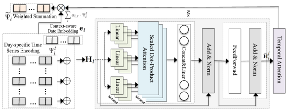
Figure 3. Temporal Pattern Aggregation Network.

While applying the autoencoder framework to map day-long time series into a low-dimensional vector, the fusion of day-specific temporal patterns presents a challenge. To address this challenge, we develop a temporal pattern aggregation network which promotes the collaboration of different day-specific temporal units for conclusive cross-time representations. Figure 3 shows the architecture of our temporal pattern aggregation network which consists of three major modules: i) context-aware time embedding module; ii) multi-head aggregation network; and iii) temporal attention network.

3.2.1. Context-Aware Time Embedding Module

From the deep autoencoder module, given the time series $\mathbf{x}_{i}$ of user $u_{i}$, we learn a set of date-ordered latent representations with size of $T$, i.e., $\mathcal{G}_{i}=\{\mathbf{g}_{i,1},...,\mathbf{g}_{i,T}\}$. In reality, different people may exhibit different wearable-sensory data distribution due to specific daily routines (Probst, Pryss, and etc, 2016). To incorporate the temporal contextual signals into our learning framework, we further augment our model with a time-aware embedding module, which utilizes the relative time difference between the last time step and each previous one. For example, given a time series with three date information $\{$2018-10-01, 2018-10-20, 2018-10-25$\}$, we generate a date duration vector as $\{24,5,0\}$ (the day duration between 2018-10-01 and 2018-10-25 is $24$ days). To avoid the occurrence of untrained long date duration in testing instances, we adopt timing signal method (Vaswani et al., 2017) to represent a non-trainable date embedding. Formally, the vector $\mathbf{e}_{t}$ of $t$-th day is derived as:

(6) $$\small e_{t,2i}=\text{sin}(\frac{t}{10000^{2i/d_{e}}});\leavevmode\nobreak\ \leavevmode\nobreak\ e_{t,2i+1}=\text{cos}(\frac{t}{10000^{2i/d_{e}}})$$

where $d_{e}$ is the embedding dimension ($2i+1$ and $2i$ are the odd and even index in the embedding vector). New context-aware latent vector $\mathbf{h}_{i,t}\in\mathbb{R}^{d_{e}}$ is generated by element-wise adding each day-specific feature representation $\mathbf{g}_{i,t}$ and date embedding $\textbf{e}_{t}$, to incorporate the temporal contextual signals into the learned embeddings.

3.2.2. Multi-Head Aggregation Network.

During the pattern fusion process, we develop a multi-head attention mechanism that is integrated with a point-wise feedforward neural network layer to automatically learn the quantitative relevance in different representation subspaces across all context-aware temporal patterns. Specifically, given the $i$-th time series, we feed all context-aware day-specific embeddings $\textbf{H}_{i}=\{\textbf{h}_{i,0},\cdots,\textbf{h}_{i,T}\}$ into a multi-head attention mechanism. Here, $M$-heads attention conducts the cross-time fusion process for $Q$ subspaces. Each $q$-th attention involves a separate self-attention learning among $\textbf{H}_{i}$ as:

(7) $$\small\widetilde{\textbf{H}}_{i}^{q}=\text{softmax}(\frac{\textbf{W}_{1}^{q}\cdot\textbf{H}_{i}(\textbf{W}_{2}^{q}\cdot\textbf{H}_{i})^{T}}{\sqrt{d_{q}}})\textbf{W}_{3}^{q}\cdot\textbf{H}_{i},$$

where $\textbf{W}_{1}^{q},\textbf{W}_{2}^{q},\textbf{W}_{3}^{q}\in\mathbb{R}^{d_{q}\times d_{e}}$ represent the learned parameters of $q$-th head attention mechanism, and $d_{q}$ is the embedding dimension of $q$-th head attention,i.e., $d_{q}=d_{e}/Q$. Then, we concatentate each learned embedding vector $\widetilde{\textbf{H}}_{i}^{q}$ from each $q$-th head attention, and further capture the cross-head correlations as follows:

(8) $$\small\widetilde{\textbf{H}}_{i}=\textbf{W}_{c}\cdot concat(\widetilde{\textbf{H}}_{i}^{1},...,\widetilde{\textbf{H}}_{i}^{Q})$$

$\mathbf{W}_{c}\in\mathbb{R}^{d_{e}\times d_{e}}$ models the correlations among head-specific embeddings. Hence, we jointly embed multi-modal dependency units into the space with the fused $\widetilde{\textbf{H}}_{i}$ using the multi-head attention network. The advantage of our multi-head attention network lies in the exploration of feature modeling in different representation spaces (Zhang et al., 2018). Then, we further feed the fused embedding $\widetilde{\textbf{H}}_{i}^{c}$ into two fully connected layers, which is defined as follows:

(9) $$\small\widetilde{\textbf{H}}_{i}^{f}=\textbf{W}_{2}^{f}\cdot\text{ReLU}(\textbf{W}_{1}^{f}\cdot\widetilde{\textbf{H}}_{i}+\textbf{b}_{1}^{f})+\textbf{b}_{2}^{f},$$

where $\textbf{W}_{1}^{f}$, $\textbf{W}_{2}^{f}$ and $\textbf{b}_{1}^{f}$, $\textbf{b}_{2}^{f}$ are the weight matrix and bias in the feed-forward layer. In our HeartSpace framework, we perform multi-head attention mechanism twice.

3.2.3. Temporal Attention Network.

To further summarize the temporal relevance, we develop a temporal attention network to learn importance weights across time. Formally, our temporal attention module can be represented as follows:

(10) $$\small\boldsymbol{\alpha}_{i}=\text{softmax}(\textbf{c}\cdot\text{Tanh}(\textbf{W}^{a}\widetilde{\textbf{H}}_{i}^{f}+\textbf{b}^{a}));\widetilde{\mathbf{g}}_{i}=\sum_{t}\alpha_{i,t}\mathbf{g}_{i,t}$$

Output $\widetilde{\textbf{H}}_{i}^{f}$ is first fed into a one fully connected layer and then together with the context vector c, it generates the importance weights $\boldsymbol{\alpha}_{i}$ through the softmax function. The aggregated embedding $\widetilde{\mathbf{g}}_{i}$ is calculated as a weighted sum of day-specific embeddings based on these learned importance weights. For simplicity, we denote our temporal pattern aggregation network as $\widetilde{\mathbf{g}}_{i}=\mathcal{A}(\mathcal{G}_{i})$.

3.3. Siamese-triplet Network Optimization Strategy

Our Siamese-triplet network optimization framework aims to enhance the encoded user feature representations with the consideration of following constraint, i.e., making representation pairs from same user closer to each other and representation pairs from different user further apart. We first define the following terms to be used in our optimization strategy.

Definition 3.

Reference Set $\mathcal{R}_{i}$: we define $\mathcal{R}_{i}$ to represent the sampled reference set of user $u_{i}$. In particular, $\mathcal{R}_{i}=\{\textbf{r}_{i}^{1},\cdots,\textbf{r}_{i}^{N^{r}}\}$ , where $N^{r}$ is size of reference set corresponding to $N^{r}$ sampled day-specific time series of $\textbf{x}_{i}$ defined in Definition 2. Each entry in $\mathcal{R}_{i}$ represents the $n_{r}$-th sampled time series from user $i$.

Definition 4.

Positive Query Set $\mathcal{P}_{i}$: we define $\mathcal{P}_{i}=\{\textbf{p}_{i}^{1},\cdots,\textbf{p}_{i}^{N^{p}}\}$ to denote the positive query set of user with size of $N^{p}$. Specifically, every entry $\textbf{p}_{i}^{n^{p}}$ represents the $n^{p}$-th sampled day-specific time series from user $u_{i}$.

Definition 5.

Negative Query Set $\mathcal{Q}_{i}$: $\mathcal{Q}_{i}=\{\textbf{q}_{i}^{1},\cdots,\textbf{q}_{i}^{N^{q}}\}$ is defined to as the negative query set for user $u_{i}$, which is the sampled $N^{q}$ day-specific time series from other users except user $u_{i}$, i.e., $u_{i^{\prime}}(i^{\prime}\neq i)$.

Based on the above definitions, given a specific user $u_{i}$, we first aggregate the elements from user $u_{i}$’s reference set $\mathcal{R}_{i}$ as: $\widetilde{\mathbf{r}}_{i}=\mathcal{A}(\mathcal{R}_{i})$, where $\mathcal{A}(\cdot)$ is the aggregation function which represents the developed temporal pattern aggregation network. Then, we compute the cosine similarity of aggregated reference element $\widetilde{\mathbf{r}}_{i}$ and each query (i.e., $\textbf{p}_{i}^{n^{p}}$ and $\textbf{q}_{i}^{n^{q}}$) from the generated positive query set $\mathcal{P}_{i}$ and negative query set $\mathcal{Q}_{i}$. Formally, the similarity estimation function $sim$ is presented as follows:

$$\small sim(\widetilde{\mathbf{r}}_{i},\mathbf{p}_{i}^{n^{p}})=\widetilde{\mathbf{r}}_{i}\cdot(\mathcal{E}(\textbf{p}_{i}^{n^{p}}))^{T};\leavevmode\nobreak\ \leavevmode\nobreak\ n^{p}\in[1,...,N^{p}];$$

(11) $$sim(\widetilde{\mathbf{r}}_{i},\mathbf{q}_{i}^{n^{q}})=\widetilde{\mathbf{r}}_{i}\cdot(\mathcal{E}(\textbf{q}_{i}^{n^{q}}))^{T};\leavevmode\nobreak\ \leavevmode\nobreak\ n^{q}\in[1,...,N^{q}];$$

where $sim(\widetilde{\mathbf{r}}_{i},\mathbf{p}_{i}^{n^{p}})\in\mathbb{R}^{1}$ and $sim(\widetilde{\mathbf{r}}_{i},\mathbf{q}_{i}^{n^{q}})\in\mathbb{R}^{1}$. By capturing the temporal consistency of each individual user $u_{i}$ and inconsistency among different users, we optimize representations that preserve inherent relationships between each user’s reference set and query set, i.e., time series embeddings from the same user are closer to each other, while embeddings from different users are more differentiated from each other. Therefore, we formally define our loss function as follows:

(12) $$\mathcal{L}_{s}^{i}=\sum_{n^{p}}\sum_{n^{q}}\mathrm{max}(0,sim(\widetilde{\mathbf{r}}_{i},\textbf{q}_{i}^{s_{q}})-sim(\widetilde{\mathbf{r}}_{i},\textbf{p}_{i}^{s_{p}})+z)$$

where $z$ is the margin between two similarities. The objective function of joint model is defined as: $\mathcal{L}_{joint}=\sum_{i}\mathcal{L}_{ae}^{i}+\lambda\mathcal{L}_{s}^{i}$, where $\lambda$ is the coefficient which control the weight of Siamese-triplet loss. The model parameters can be derived by minimizing the loss function. We use Adam optimizer to learn the parameters of HeartSpace. The model optimization process is summarized in Algorithm 1.

1

2

3

4

5

6

7

Input: User set $\mathcal{U}$; reference set size $N^{r}$, positive query size $N^{p}$, negative query size $N^{q}$

8 Initialize all parameters;

9 while not converge do

10       sample a set of users from user set $\mathcal{U}$;

11       foreach user $u_{i}$ do

12             sample support set $\mathcal{R}_{i}$ and positive set $\mathcal{P}_{i}$;

13             sample negative set $\mathcal{Q}_{i}$;

14             feed each entry in $\mathcal{R}_{i}$, $\mathcal{P}_{i}$ and $\mathcal{Q}_{i}$ into autoencoder to get daily representations and compute $\mathcal{L}_{ae}^{i}$;

15             aggregate support set $\mathcal{R}_{i}$ and derive $\mathcal{L}_{s}^{i}$;

16            

17       end foreach

18      update all parameters w.r.t $\mathcal{L}_{joint}=\sum_{i}\mathcal{L}_{ae}^{i}+\mathcal{L}_{s}^{i}$;

19      

20 end while

Algorithm 1 The Model Inference of HeartSpace.

Unsupervised and semi-supervised learning scenarios. HeartSpace is a general representation learning model that is flexible for both unsupervised (without labeled instances) and semi-supervised (limited number of labeled instances) learning. In semi-supervised learning, given the labeled time series and its target value, we take the learned representation vector as the input of a single-layer perceptrons with a combined loss function, i.e.integrate the joint objective function $\mathcal{L}_{joint}$ with the loss function based on cross-entropy (categorical values) or MSE (quantitative values).

4. Evaluation

We comprehensively evaluate HeartSpace on several inference and prediction tasks: user identification, personality prediction, demographic inference and job performance prediction. Our longitudinal real-world data comes from two different studies leveraging two different sensors and different population groups, thus allowing us to carefully vet and validate our findings. To robustly evaluate the accuracy and generalization of embeddings learned by HeartSpace, within the context of the aforementioned prediction tasks, we aim to answer the following questions:

• Q1: How does HeartSpace perform compared with state-of-the-art representation learning methods for the wearable-sensory time series, as represented by heart rate?

• Q2: How is the performance of HeartSpace with respect to different training/testing time periods in user identification?

• Q3: How do different components of HeartSpace (i.e., deep autoencoder module, multi-head aggregation network and Siamese-triplet network optimization strategy) contribute to the HeartSpace performance?

• Q4: How do the key hyperparameters (e.g., reference set size $S_{r}$ and embedding dimension $d_{e}$) affect HeartSpace performance?

• Q5: How does HeartSpace lend itself for visualizing similarities and differences among individuals (interpretation)?

4.1. Experimental Settings

4.1.1. Data Description.

We considered the heart rate time series data from two research projects . For the purpose of the paper, we shall notate them based on the sensor: Garmin and Fitbit, respectively.

Garmin Heart Rate Data. This dataset comes from an on-going research study of workplace performance which measures the physiological states of employees in multiple companies. This dataset is collected from 578 participants (age between 21 to 68) by Garmin band from March 2017 to August 2018. Each measurement is formatted as (user id, heart rate, timestamp).

Fitbit Heart Rate Data. We collect this dataset from a research project at a University which aims to collect survey and wearable data from an initial cohort of 698 students (age between 17 to 20) who enrolled in the Fall semester of 2015. This dataset is collected by Fitbit Charge during the 2015/2016 and 2016/2017 academic years.

4.1.2. Data Distribution.

Figure 4 shows the distribution of wearable-sensory time series in terms of time series length $J_{i}$ and completeness degree (i.e., the ratio of non-zero elements in day-specific time series $\textbf{x}_{i}^{t}$) on both Garmin and Fitbit heart rate data. As depicted in Figure 4 (a) and (b), different datasets have different time series distributions. Furthermore, Figure 4 (c) and (d) reveals that data incompleteness is ubiquitous, e.g., there exists more than 20% day-specific time series with data incompleteness $<0.8$, which poses a further challenge for HeartSpace. These observations are the main motivation to develop a temporal pattern aggregation network and a dual-stage gating mechanism for handling variable-length time series with incomplete data.

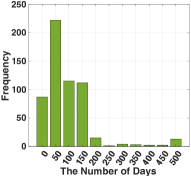
(a) Garmin Data

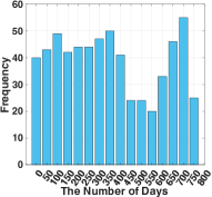
(b) Fitbit Data

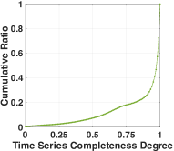
(c) Garmin Data

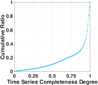
(d) Fitbit Data

Figure 4. Distribution of Time Series Length (a-b) and Completeness Degree (c-d).

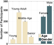
(a) User Demographic

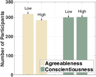
(b) User Personality

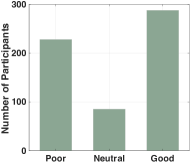
(c) Work Performance

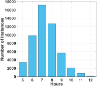
(d) Sleep Duration

Figure 5. Data Statistics w.r.t User Demographics, Personality and Sleep Duration.

4.1.3. Methods for Comparison.

To justify the effectiveness of HeartSpace for representation learning on wearable-sensory data, we compared it with the following contemporary representation learning methods:

• Convolutional Autoencoder (CAE) (Bascol, Emonet, and etc, 2016): CAE is a representation learning framework by applying convolutional autoencoder to map the time series patterns into latent embeddings.
  

• Deep Sequence Representation (DSR) (Amiriparian et al., 2018): DSR is a general-purpose encoder-decoder feature representation model on sequential data with two deep LSTMs, one to map input sequence to vector space and another to map vector to the output sequence.
  

• Multi-Level Recurrent Neural Networks (MLR) (Cheng et al., 2017): MLR is a multi-level feature learning model to extract low- and mid-level features from raw time series data. RNNs with bidirectional-LSTM architectures are employed to learn temporal patterns.

• Sequence Transformer Networks (STN) (Oh, Wang, and Wiens, 2018): STN is an end-to-end trainable method for learning structural information of clinical time-series data, to capture temporal and magnitude invariances.
  

• Wave2Vec (Yuan, Xun, and others, 2019): It is a sequence representation learning framework using skip-gram model by considering sequential contextual signals. Specifically, it takes the one-by-one data points that surround the target point within a defined window, to feed into a neural network for appear probability prediction. The window size and number of negative samples is set as 1 and 4, respectively.
  

• DeepHeart (Bhattacharjee et al., 2018): DeepHeart is a deep learning approach which models the temporal pattern of heart rate time-series data with the integration of the convolutional and recurrent neural network architecture.
  

The initial parameter settings for each of the above methods are consistent with their original papers.

4.1.4. Evaluation Protocols.

To measure the effectiveness of HeartSpace for representation learning on heart rate data in downstream applications, we conduct multiple tasks, including user identification, personality prediction, user demographic inference, job performance prediction and sleep duration prediction. These tasks reflect inferring qualified self from quantified self. We summarize the details for five different tasks as follows:

• User Identification: In the user identification evaluation, each of the aforementioned methods learns a mapping function to encode each of the day-specific time series data into a low-dimensional representation vector. Then, given multiple day-specific time series data from one user and an unknown day-specific time series, the task is to predict whether the unknown time series is collected from the same user of the multiple day-specific time series. Specifically, we first map day-specific time series to embedding vector by utilizing each of the aforementioned methods. Then we aggregate embedding vectors of multiple day-specific time series to generate the reference vector. We apply mean-pooling operation on baselines and temporal aggregation network on HeartSpace during the aggregation process. After that, we take the element-wise product between the reference vector and the embedding vector of the single day-specific time series as the input. Here, we adopt a logistic regression classifier to learn the model from the training data and generate the prediction. The True Positives and True Negatives are the heart rate series that are correctly identified for user $u_{i}$ or not, respectively, by the classifier. The False Positives and False Negatives are the heart rate series that are misclassified as belonging to user $u_{i}$ or not, respectively.

• Personality Prediction: We considered two personality attributes of the participants, namely Conscientiousness and Agreeableness. We considered a classification task of a binary prediction on these attributes — high or low for each participant $u_{i}$ (McCrae and John, 1992).In this task, the goal was to evaluate whether the embeddings learned from the heart rate are effective predictors of the personality types. We use the Logistic Regression classifier to make the prediction with the embedding as the feature space. The True Positives and True Negatives are the participants that are correctly classified by the classification method as high- and low-level, respectively. The False Positives and False Negatives are the high- and low-level participants that are misclassified, respectively. We only use the Garmin data for this task, as we only survey personality attributes for the subjects in the pool.

• User Demographic Inference: We evaluate whether user demographics, such as gender and age are predictable by using a similar experimental construct as in (Dong et al., 2014). The age information is categorized into four categories (i.e., Young: from 18 to 24, Young-Adult: from 23 to 34, Middle-age: from 39 to 49, senior: from 49 to 100).

• Job Performance Prediction: We also evaluate the performance of predicting each participant’s job performance (Individual Task Performance), which is categorized into three types, i.e., good, neutral, poor (Conway, 1999). We only use the Garmin data for this task, as we only collect job performance information for the subjects in the Garmin pool.

• Sleep Duration: We further conduct the sleep duration estimation task to evaluate the quality of learned representations. We utilize the Linear Regression model which takes the embedding vectors of the target day-long time series as the input and predicts the sleep duration of that day as the output.

We evaluate user identification and personality prediction tasks in terms of F1-score, Accuracy and AUC. In addition, the user demographic inference and job performance prediction tasks, given multi-class scenario, are evaluated using Macro-F1 and Micro-F1. The sleep duration task is evaluated in terms of MSE and MAE.

4.1.5. Training/Test Data Split.

We summarize the details of training/test data partition for different evaluation tasks as follows:

• For demographic inference, personality prediction and job performance prediction task, we use the entire heart rate data for learning time series embeddings, and split the labels with $60\%$, $10\%$ and $30\%$ for training, validation and test, respectively.

• For the user identification task, wesplit the datasets in chronological order. We first use Garmin data from March to Dec in 2017 (10 months), to learn parameters of HeartSpace for time series embedding in an unsupervised fashion. Then, we leverage the data from Jan 2018 to Aug 2018 to evaluate the user identification performance based on the generated embeddings from the learned model. Specifically, we perform the training/test process over the period of Jan 2018 to Aug 2018 with a sliding window of two months, i.e., (Jan $\rightarrow$ training, Feb $\rightarrow$ test);…; (Jul $\rightarrow$ training, Aug $\rightarrow$ test). The training month provides the labels to learn the classifier and the test month is used to evaluate the prediction accuracy. Irrespective of the training/ test month combination, the model parameters are learned on the basis of 2017 data in an unsupervised fashion. This allows us to also consider the generalization of performance over time. Moreover, to ensure the fairness of performance comparison, the day-long time series of users shown in the test set are not visible in the training set using our partition strategy. The training/test partition method on Fitbit data is similar as the Garmin data.

4.2. Reproducibility

We implemented all the deep learning baselines and the proposed HeartSpace framework with Tensorflow. For the sake of fair comparison, all experiments are conducted across all participants in the testing data and the average performance is reported. Furthermore, the validation was run ten times and the average performance numbers are reported. In our experiments, we set the embedding dimension, the support size, positive sampling size, negative sampling size as 64, 6, 2, 4, respectively. The margin value is set as 1 and the Siamese-triplet weight is set as 4. We utilized the Glorot initialization (Glorot and Bengio, 2010) and grid search (Grover and Leskovec, 2016) strategies for hyperparameter initialization and tuning of all compared methods. The early stopping (Raskutti, Wainwright, and Yu, 2014) is adopted to terminate the training process based on the validation performance. After the parameter tuning on all baselines, we reported their best performance in the evaluation results. During the model learning process, we used the Adam optimizer, where the batch size and learning rate were set as 64 and 0.001, respectively.

Table 1. User identification performance in terms of F1-score, Accuracy and AUC.

Data	Garmin Heart Rate Data
Month	Feb			Apr			June			Aug
Method	F1	Acc.	AUC	F1	Acc.	AUC	F1	Acc.	AUC	F1	Acc.	AUC
CAE	0.658	0.650	0.711	0.680	0.672	0.737	0.660	0.669	0.742	0.684	0.698	0.770
DSR	0.649	0.643	0.692	0.685	0.670	0.727	0.708	0.708	0.784	0.694	0.696	0.772
MLR	0.652	0.637	0.685	0.689	0.670	0.731	0.707	0.702	0.773	0.703	0.704	0.776
STN	0.616	0.572	0.598	0.732	0.737	0.816	0.750	0.758	0.843	0.733	0.740	0.817
Wave2Vec	0.743	0.751	0.832	0.796	0.803	0.884	0.816	0.822	0.901	0.824	0.830	0.909
DeepHeart	0.731	0.738	0.812	0.753	0.757	0.834	0.766	0.773	0.855	0.750	0.756	0.844
HeartSpace	0.764	0.764	0.841	0.805	0.806	0.890	0.830	0.833	0.913	0.858	0.862	0.935
Data	Fitbit Heart Rate Data
Month	Feb			Apr			June			Aug
Method	F1	Acc.	AUC	F1	Acc.	AUC	F1	Acc.	AUC	F1	Acc.	AUC
CAE	0.579	0.577	0.602	0.596	0.594	0.641	0.602	0.587	0.634	0.606	0.599	0.638
DSR	0.647	0.646	0.696	0.630	0.617	0.654	0.619	0.612	0.671	0.613	0.598	0.641
MLR	0.643	0.639	0.697	0.626	0.624	0.680	0.6737	0.665	0.740	0.659	0.649	0.705
STN	0.712	0.718	0.778	0.687	0.689	0.749	0.686	0.681	0.746	0.729	0.727	0.787
Wave2Vec	0.778	0.778	0.862	0.777	0.777	0.857	0.771	0.770	0.857	0.813	0.812	0.893
DeepHeart	0.678	0.680	0.746	0.715	0.718	0.787	0.719	0.722	0.791	0.715	0.714	0.784
HeartSpace	0.799	0.797	0.869	0.804	0.803	0.886	0.786	0.782	0.868	0.833	0.831	0.914

Table 2. User demographic inference results. Mic-F1: Micro-F1; Mac-F1: Macro-F1

Demographic	Age		Gender
Metric	Mic-F1	Mac-F1	Mic-F1	Mac-F1
CAE	0.517	0.364	0.674	0.655
DSR	0.505	0.259	0.645	0.633
MLR	0.523	0.270	0.645	0.628
STN	0.529	0.346	0.627	0.622
Wave2Vec	0.546	0.354	0.657	0.645
DeepHeart	0.494	0.266	0.639	0.618
HeartSpace	0.558	0.377	0.703	0.672

4.3. Performance Comparison (Q1 and Q2)

4.3.1. User Identification

Table 1 shows the user identification performance on both datasets. We can observe that HeartSpace achieves the best performance and obtains significant improvement over state-of-the-art methods in all cases. This sheds lights on the benefit of HeartSpace, which effectively captures the unique signatures of individuals. Although other neural network-based methods preserve the temporal structural information to learn latent representations for each individual time series, they ignore the variable-length and incompleteness of wearable-sensory data, which reveals the practical difficulties in learning accurate models across non-continuous time steps.

To make thorough evaluation, we conduct comparison experiment of HeartSpace and all baselines across different training and test time periods (e.g., Feb, Apr, Jun and Aug). We can note that the best performance is consistently achieved by HeartSpace with different forecasting time periods, which reflects the robustness of HeartSpace in learning the latent representations over time.

4.3.2. Demographic Inference

The demographic inference performance comparison between HeartSpace and other competitive methods on the Garmin heart rate data is shown in Table 2. We can note that our HeartSpace outperforms other baselines in inferring users’ age and gender information, which further demonstrate the efficacy of our HeartSpace in learning significantly better time series embeddings than existing state-of-the-art methods. Similar results can be observed for the Fitbit heart rate data. In summary, the advantage of HeartSpace lies in its proper consideration of comprehensive temporal pattern fusion for time series data.

4.3.3. Personality Prediction

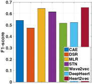
(a) Conscientiousness

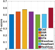
(b) Agreeableness

Figure 6. Personality detection results.

Figure 6 shows the personality prediction results on two different categories (i.e., Agreeableness and Conscientiousness). We can observe that HeartSpace achieves the best performance in all personality cases. The performance is followed by DSR which extracts both multi-level temporal features during the representation learning process. This further verifies the utility of temporal pattern fusion in mapping time series data into common latent space.

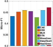
(a) Micro-F1

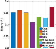
(b) Macro-F1

Figure 7. Job performance prediction results.

4.3.4. Job Performance Prediction

The results of job performance prediction are presented in Figure 7. In these figures, we can notice that HeartSpace achieves the best performance in terms of Macro-F1 and Micro-F1.

4.3.5. Sleep Duration Inference

We further evaluate the proposed HeartSpace with the application of forecasting the sleep duration of people. The performance evaluation results (measured by MSE and MAE) are presented in Figure 8. We can observe that significant performance improvements are consistently obtained by HeartSpace over state-of-the-art baselines, which further validates the effectiveness of HeartSpace.

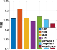
(a) MSE

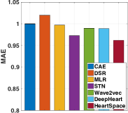
(b) MAE

Figure 8. Sleep duration forecasting results.

4.4. Model Ablation: Component-Wise Evaluation of HeartSpace (Q3)

We also aim to get a better understanding of key components of HeartSpace. In our evaluation, we consider three variants of the proposed method corresponding to different analytical aspects:

• Effect of Siamese-triplet Network HeartSpace-s. A simplified version of HeartSpace which does not include Siamese-triplet network to model intra- and inter-time series inter-dependencies.

• Effect of Deep Autoencoder Module. HeartSpace-a. A simplified version of HeartSpace without deep autoencoder module, i.e., only consider $\mathcal{L}_{s}$ (Siamese-triplet Network) in the loss function.

• Effect of Multi-head Attention Network. HeartSpace-h: A variant of HeartSpace without the multi-head attention network to learn the weights of different day-specific temporal patterns.

We report the results in Figure 9. Notice that the full version of HeartSpace achieves the best performance in all cases, which suggests: (i) The efficacy of the designed Siamese-triplet network optimization strategy for preserving structural information of implicit intra- and inter-time series correlations. (ii) The effectiveness of HeartSpace in capturing complex temporal dependencies across time steps for variable-length sensor data. (iii) The effectiveness of HeartSpace in exploring feature modeling in different representation spaces during our pattern fusion process. As such, it is necessary to build a joint framework to capture multi-dimensional correlations in wearable-sensory time series representation learning.

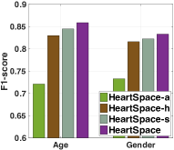
(a) User Identification

(b) Demographic Inference

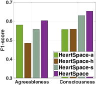
(c) Personality Prediction

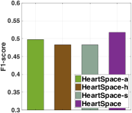
(d) Job Performance Prediction

Figure 9. Evaluation on HeartSpace variants.

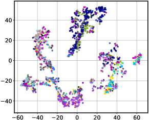
(a) DeepHeart

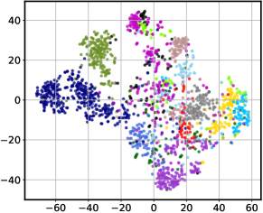
(b) HeartSpace

Figure 10. Embedding visualizations of HeartSpace v.s. DeepHeart. 2D t-SNE projections of the 64D embeddings of all day-specific time series from 15 participants on the Garmin heart rate data. Each color indicates an individual user.

4.5. Hyperparameter Studies (Q4)

To investigate the robustness of HeartSpace, we examined how the different choices of five key parameters affect the performance of HeartSpace. Figure 11 shows the evaluation results as a function of one selected parameter when fixing others. Overall, we observe that HeartSpace is not strictly sensitive to these parameters and is able to reach high performance under a cost-effective parameter choice, which demonstrates the robustness of HeartSpace.

Furthermore, we can observe that the increase of prediction performance saturates as the representation dimensionality increases. This is because: at the beginning, a larger value of embedding dimension brings a stronger representation power for the recent framework, but the further increase of dimension size of latent representations might lead to the overfitting issue. In our experiments, we set the dimension size as 64 due to the consideration of the performance and computational cost. We can observe that both the positive query set size and negative query set size, as well as siamese triple loss coefficient have a relatively low impact on the model performance.

Figure 11. Hyperparameter Studies in terms of F1-score.

4.6. Case Study: Visualization (Q5)

We employ the TensorFlow embedding projector to further visualize the low-dimensional time series representations learned by HeartSpace and one selected baseline (DeepHeart) on Garmin heart rate dataset. Figure 10 shows the visualization of day-specific time series embeddings from randomly selected 15 users. We can observe that the embeddings from the same user could be identified by our HeartSpace and cluster them closer than other embeddings, while the embeddings learned by DeepHeart of different users are mixed and cannot be well identified. Therefore, our model generates more accurate feature representations of user’s time series data and is capable of preserving the unique signatures of each individual, which can then be leveraged for similarity analyses.

5. Related Work

Representation Learning Models. With the advent of deep learning techniques, significant effort has been devoted to developing neural network-based representation learning models on various data. For the word representation learning, there exist a good amount of literature on designing techniques by considering word context in a document, such as word2vec (Mikolov et al., 2013) and Glove (Pennington, Socher, and Manning, 2014). Many follow-up works extend the basic framework to learn latent representations on multimedia data (Ramanathan et al., 2015; Goroshin et al., 2015) and network data (Tu et al., 2018; Grover and Leskovec, 2016), in order to capture frame-level temporal dependency and network structural information, respectively. For example, node2vec (Grover and Leskovec, 2016) proposes to learn node embeddings based on random walk. However, the wearable-sensory time series representation learning remains to be a critical but largely unsolved question. This work proposes a principled framework to address this challenge by automatically preserving the underlying structure of dynamic temporal patterns of wearable-sensory time series data.

Deep Learning for Healthcare Applications. With the advent of deep learning techniques, many deep neural network frameworks have been proposed to address various challenges in healthcare informatics (Bai et al., 2018; Ma, Gao, and others, 2018; Cao et al., 2017; Suhara, Xu, and Pentland, 2017; Choi, Bahadori, and others, 2017). For example, Cao et al.(Cao et al., 2017) proposed an end-to-end deep architecture for the prediction of human mood. Bai et al.(Bai et al., 2018) modeled sequential patient data and predict future clinical events. This work furthers this direction of investigation by proposing a general time series representation learning framework to capture hierarchical structural correlations exhibited from human heart rate data, which cannot be handled by previous models.

Representation Learning on wearable-sensory Data. A handful of studies (Ballinger et al., 2018; Amiriparian et al., 2018; Lehman et al., 2018) have investigated the representation learning on wearable-sensory data. Ballinger et al.(Ballinger et al., 2018) proposed a semi-supervised learning method to detect health conditions. Amiriparian et al.(Amiriparian et al., 2018) explored the deep feature representations to aid the diagnosis of cardiovascular disorders with sequence to sequence autoencoders. While these pioneering studies have demonstrated the effectiveness of representation learning on wearable-sensory data, they do not address our problem of designing a unified model that dynamically captures the evolving temporal characteristics from wearable-sensory time series with variable-length.

6. Conclusion

In this paper, we presented HeartSpace, a novel time series representation learning method for wearable-sensory data that addresses several challenges stemming from such data and also overcomes the limitations of current state-of-the-art approaches, including dealing with incomplete and variable length time series, intra-sensor / individual variability, and absence of ground truth. HeartSpace first learns latent representation to encode temporal patterns of individual day-specific time series with a deep autoencoder model. Then, an integrative framework of a pattern aggregation network and a Siamese-triplet network optimization maps variable-length wearable-sensory time series into the common latent space such that the implicit intra-series and inter-series correlations well preserved. Extensive experiments on real-world data, representing different sensor and subjects’ distribution, demonstrate that the latent feature representations learned by HeartSpace are significantly more accurate and generalizable than the contemporary methods.

References

- Amiriparian et al. (2018) Amiriparian, S.; Schmitt, M.; Cummins, N.; Qian, K.; Dong, F.; and Schuller, B. 2018. Deep unsupervised representation learning for abnormal heart sound classification. In EMBC, 4776–4779. IEEE.
- Bai et al. (2018) Bai, T.; Zhang, S.; Egleston, B. L.; and Vucetic, S. 2018. Interpretable representation learning for healthcare via capturing disease progression through time. In KDD, 43–51. ACM.
- Ballinger et al. (2018) Ballinger, B.; Hsieh, J.; Singh, A.; et al. 2018. Deepheart: Semi-supervised sequence learning for cardiovascular risk prediction. In IJCAI.
- Bascol, Emonet, and etc (2016) Bascol, K.; Emonet, R.; and etc. 2016. Unsupervised interpretable pattern discovery in time series using autoencoders. In SSPR, 427–438. Springer.
- Bhattacharjee et al. (2018) Bhattacharjee, T.; Datta, S.; Das, D.; Choudhury, A. D.; Pal, A.; and Ghosh, P. K. 2018. A heart rate driven kalman filter for continuous arousal trend monitoring. In EMBC, 3572–3577. IEEE.
- Cao et al. (2017) Cao, B.; Zheng, L.; Zhang, C.; Yu, P. S.; Piscitello, A.; Zulueta, J.; Ajilore, O.; Ryan, K.; and Leow, A. D. 2017. Deepmood: modeling mobile phone typing dynamics for mood detection. In KDD, 747–755. ACM.
- Cheng et al. (2017) Cheng, M.; Sori, W. J.; Jiang, F.; Khan, A.; and Liu, S. 2017. Recurrent neural network based classification of ecg signal features for obstruction of sleep apnea detection. In CSE, volume 2, 199–202. IEEE.
- Choi, Bahadori, and others (2017) Choi, E.; Bahadori, M. T.; et al. 2017. Gram: graph-based attention model for healthcare representation learning. In KDD, 787–795. ACM.
- Conway (1999) Conway, J. M. 1999. Distinguishing contextual performance from task performance for managerial jobs. Journal of applied Psychology 84(1):3.
- Doetsch, Golik, and Ney (2017) Doetsch, P.; Golik, P.; and Ney, H. 2017. A comprehensive study of batch construction strategies for recurrent neural networks in mxnet. arXiv preprint arXiv:1705.02414.
- Dong et al. (2014) Dong, Y.; Yang, Y.; Tang, J.; and etc. 2014. Inferring user demographics and social strategies in mobile social networks. In KDD, 15–24. ACM.
- Glorot and Bengio (2010) Glorot, X., and Bengio, Y. 2010. Understanding the difficulty of training deep feedforward neural networks. In AISTATS, 249–256.
- Goroshin et al. (2015) Goroshin, R.; Bruna, J.; Tompson, J.; and etc. 2015. Unsupervised learning of spatiotemporally coherent metrics. In ICCV, 4086–4093.
- Grover and Leskovec (2016) Grover, A., and Leskovec, J. 2016. node2vec: Scalable feature learning for networks. In KDD, 855–864. ACM.
- Hu, Shen, and Sun (2018) Hu, J.; Shen, L.; and Sun, G. 2018. Squeeze-and-excitation networks. In CVPR, 7132–7141.
- Lehman et al. (2018) Lehman, E. P.; Krishnan, R. G.; Zhao, X.; Mark, R. G.; and Li-wei, H. L. 2018. Representation learning approaches to detect false arrhythmia alarms from ecg dynamics. In MLHC, 571–586.
- Liu et al. (2015) Liu, B.; Li, J.; Chen, C.; and etc. 2015. Efficient motif discovery for large-scale time series in healthcare. TII 11(3):583–590.
- Liu et al. (2016) Liu, X.; Liu, L.; Simske, S. J.; and etc. 2016. Human daily activity recognition for healthcare using wearable and visual sensing data. In ICHI, 24–31. IEEE.
- Ma, Gao, and others (2018) Ma, F.; Gao, J.; et al. 2018. Risk prediction on electronic health records with prior medical knowledge. In KDD, 1910–1919. ACM.
- Manashty, Light, and Soleimani (2018) Manashty, A.; Light, J.; and Soleimani, H. 2018. A concise temporal data representation model for prediction in biomedical wearable devices. Internet of Things Journal.
- McCrae and John (1992) McCrae, R. R., and John, O. P. 1992. An introduction to the five-factor model and its applications. Journal of personality 60(2):175–215.
- Mikolov et al. (2013) Mikolov, T.; Sutskever, I.; Chen, K.; and etc. 2013. Distributed representations of words and phrases and their compositionality. In NIPS, 3111–3119.
- Nakamura, Takimoto-Inose, and etc (2018) Nakamura, K.; Takimoto-Inose, A.; and etc. 2018. Cross-modal perception of human emotion in domestic horses. Scientific Reports 8(1):8660.
- Ni, Muhlstein, and McAuley (2019) Ni, J.; Muhlstein, L.; and McAuley, J. 2019. Modeling heart rate and activity data for personalized fitness recommendation.
- Oh, Wang, and Wiens (2018) Oh, J.; Wang, J.; and Wiens, J. 2018. Learning to exploit invariances in clinical time-series data using sequence transformer networks. Machine Learning for Healthcare.
- Op De Beéck, Meert, and others (2018) Op De Beéck, T.; Meert, W.; et al. 2018. Fatigue prediction in outdoor runners via machine learning and sensor fusion. In KDD, 606–615. ACM.
- Pennington, Socher, and Manning (2014) Pennington, J.; Socher, R.; and Manning, C. 2014. Glove: Global vectors for word representation. In EMNLP, 1532–1543.
- Probst, Pryss, and etc (2016) Probst, T.; Pryss, R.; and etc. 2016. Emotional states as mediators between tinnitus loudness and tinnitus distress in daily life: Results from the trackyourtinnitus application. Scientific Reports 6:20382.
- Ramanathan et al. (2015) Ramanathan, V.; Tang, K.; Mori, G.; and Fei-Fei, L. 2015. Learning temporal embeddings for complex video analysis. In ICCV, 4471–4479.
- Raskutti, Wainwright, and Yu (2014) Raskutti, G.; Wainwright, M. J.; and Yu, B. 2014. Early stopping and non-parametric regression: an optimal data-dependent stopping rule. JMLR 15(1):335–366.
- Srivastava, Greff, and Schmidhuber (2015) Srivastava, R. K.; Greff, K.; and Schmidhuber, J. 2015. Training very deep networks. In NIPS, 2377–2385.
- Suhara, Xu, and Pentland (2017) Suhara, Y.; Xu, Y.; and Pentland, A. 2017. Deepmood: Forecasting depressed mood based on self-reported histories via recurrent neural networks. In WWW, 715–724. ACM.
- Sun, Leng, and etc (2015) Sun, Y.; Leng, B.; and etc. 2015. A novel wavelet-svm short-time passenger flow prediction in beijing subway system. Neurocomputing 166:109–121.
- Tu et al. (2018) Tu, K.; Cui, P.; Wang, X.; Yu, P. S.; and Zhu, W. 2018. Deep recursive network embedding with regular equivalence. In KDD, 2357–2366. ACM.
- Vaswani et al. (2017) Vaswani, A.; Shazeer, N.; Parmar, N.; Uszkoreit, J.; and etc. 2017. Attention is all you need. In NIPS, 5998–6008.
- Wang et al. (2016) Wang, P.; Guo, J.; Lan, Y.; and Xu, J. 2016. Your cart tells you: Inferring demographic attributes from purchase data. In WSDM, 173–182. ACM.
- Wang et al. (2018a) Wang, J.; Zhang, J.; Bao, W.; and etc. 2018a. Not just privacy: Improving performance of private deep learning in mobile cloud. In KDD, 2407–2416. ACM.
- Wang et al. (2018b) Wang, L.; Zhang, W.; He, X.; and Zha, H. 2018b. Supervised reinforcement learning with recurrent neural network for dynamic treatment recommendation. In KDD, 2447–2456. ACM.
- Yang, Dumont, and etc (2006) Yang, P.; Dumont, G.; and etc. 2006. Adaptive change detection in heart rate trend monitoring in anesthetized children. TBE 53(11):2211–2219.
- Yuan, Xun, and others (2019) Yuan, Y.; Xun, G.; et al. 2019. Wave2vec: Deep representation learning for clinical temporal data. Neurocomputing 324:31–42.
- Zhang et al. (2018) Zhang, J.; Shi, X.; Xie, J.; and etc. 2018. Gaan: Gated attention networks for learning on large and spatiotemporal graphs.
- Zhu et al. (2018) Zhu, Y.; Yeh, C.-C. M.; Zimmerman, Z.; and etc. 2018. Matrix profile xi: Scrimp++: Time series motif discovery at interactive speeds. In ICDM, 837–846. IEEE.