Abstract

We study Euclidean wormholes in the framework of the Ho$\check{\rm r}$ava-Lifshitz theory of gravity. Euclidean wormholes first appeared in the Euclidean path integral approach to quantum gravity. In a more general way, Hawking and Page interpreted such configurations as solutions to the Wheeler-DeWitt equation with appropriate boundary conditions. We use the projectable version of Ho$\check{\rm r}$ava-Lifshitz gravity to obtain the Wheeler-DeWitt equation of a minisuperspace model considering a closed Friedmann Universe plus a massless scalar field. For large values of the scale factor we find that the solution of the Wheeler-DeWitt equation coincides with the one obtained by Hawking. Whereas in the limit corresponding to the early Universe we find a new set of solutions, which agree with the Hawking and Page boundary conditions for wormholes.

1 Introduction

It is well known that in the quantum field theoretic description of Einstein’s gravity one founds ultraviolet (UV) divergences. The presence of these UV divergences has its origin in the fact that Newton’s constant has mass dimension $\left[G_{N}\right]=-2$. That means that the gravitational interaction may be described by an effective field theory, in which case it would require an UV completion. In Ref. [1] Ho$\check{\rm r}$ava proposed one possible UV completion of Einstein theory. The basic idea of Ho$\check{\rm r}$ava’s theory is to improve the UV behavior of gravity by adding higher-order terms in the spatial component of the curvature to the Einstein-Hilbert action. The result is a theory of gravity in 3+1 dimensions that is power-counting renormalizable and whose equations of motion are of second order in time, avoiding the presence of ghosts. In this scenario Ho$\check{\rm r}$ava’s idea was to follow some work of Lifshitz in condensed matter physics regarding the consideration of an anisotropic scaling of space and time

$$t\rightarrow b^{z}t,\qquad x^{i}\rightarrow bx^{i},\qquad(i=1,2,\ldots,d)$$ (1)

This scaling is known as Lifshitz scaling, where $b$ is a constant, $d$ denotes the spatial dimension of spacetime, and $z$ is a number called the dynamical critical exponent, which dictates the degree of anisotropy between space and time. It is clear that Lorentz symmetry is broken for $z\neq 1$ in the UV and it is recovered only when $z=1$, which occurs at low energies in the infrared (IR).

It is important to point out that the Lifshitz scaling does not respect the full invariance under diffeomorphisms present in general relativity (GR). Thus one has to introduce a more restricted reparametrization of spacetime which respect the foliation ${\cal F}$ into space and time

$$t\mapsto\tilde{t}(t),\quad x^{i}\mapsto\tilde{x}^{i}(t,x^{i}).$$ (2)

This remaining redundancy is called foliation-preserving-diffeomorphisms (or ${\cal F}$Diff for short) because the spatial diffeomorphisms are the ones that remain unchanged. In other words, it is chosen a preferred time. This proposal constitutes the so called Ho$\check{\rm r}$ava-Lifshitz (HL) theory of gravity and it can be regarded as an extension of GR to higher energies (for some reviews on the subject, see [2, 3, 4, 5] and references therein).

In this article we will work in one of the versions of the HL theory known as the projectable theory. It is known that this theory has a unphysical scalar degree of freedom which leads to a perturbative IR instability [3]. For the projectable case this IR instability was studied in Refs. [5, 6, 7]. In these references it is found that in the limit $\lambda\to 1$, the resulting theory is GR coupled to the scalar model describing dark matter (DM). In the specific case of quantum cosmology in the minisuperspace approach for a homogeneous and isotropic metric of the Fiedmann-Lemaitre-Robertson-Walker (FLRW) type, the projectable model leads to a Friedmann equation including a DM component through the additional scalar mode. From the view point of the canonical approach to gravity, projectable and non-projectable models differ in the local nature of the Hamiltonian constraint for the non-projectable case and non-local one for the projectable case. In the non-projectable model the scalar degree of freedom is absent. Consequently, if one is only interested in solving the Hamiltonian constraint (i.e. the Wheeler-DeWitt (WDW) equation) for a FLRW metric, both: projectable and non-projectable models will give the same results and the IR perturbative instability is not evident. Some of the papers describing some solutions of Ho$\check{\rm r}$ava-Lifshitz’s gravity in quantum cosmology in the minisuperspace are [8, 9, 10, 11, 12, 13, 14].

On the other hand, the idea of wormhole solution in GR was suggested by Wheeler, the ideas is that the topology of spacetime may fluctuate on scales of the order of the Planck length ($\sim 10^{-33}$ cm) giving rise to wormhole configurations [15, 16]. These objects are defined as finite-action solutions to the equations of motion of the classical Euclidean Einstein field equations, which is why they are also called gravitational instantons. In other words, they are Euclidean metrics that describe two asymptotically flat regions joined by a narrow tube or throat. For an account on some of these subjects in Euclidean gravity, see for instance, [17].

The interest on Euclidean wormhole physics peaked in the late 1980s after Giddings and Strominger found a gravitational instanton solution by considering a model of an axionic field (a 3-form) coupled to gravity [18]. The importance of this solution was appreciated mainly due to the application of wormholes to the cosmological constant problem. Such an idea was pursued by Coleman who used the saddle point approximation in the path integral approach to show that one of the possible effects of wormholes was to set the value of the cosmological constant to zero [19]. Later Hawking also argued that macroscopic wormholes might be responsible for the mechanism of black hole evaporation. In this picture, baby universes are pinched-off from some region of our Universe carrying away information [20]. Euclidean wormholes have plenty of implications on particle physics and cosmology [21], and for that reason a renewal interest has started to appear in recent years. In particular, Euclidean wormholes (or more specifically, Giddings-Strominger axionic wormholes) seem to satisfy the Weak Gravity Conjecture [22], which gives support to its physical relevance.

For some time wormholes were only studied as solutions to the Euclidean field equations using a semiclassical treatment. Such solutions exist only for specific kinds of matter. Thus it seems more natural that their importance rely in microscopic physics and one shall to study them in a quantum mechanical setting. This approach was followed by Hawking and Page in [23]. They regarded wormholes as solutions to the WDW equation obeying the so called Hawking-Page boundary conditions: $({\rm a})$ The wave function needs to be exponentially damped for large 3-geometries; $({\rm b})$ It is regular as the 3-geometry collapses to zero.

The foliation of spacetime in constant time hypersurfaces is known as the Arnowitt, Deser and Misner (ADM) [24]) decomposition of spacetime [24]. It is also the starting point of quantum cosmology, where the quantum dynamics is governed by the WDW equation (for a review of quantum cosmology, see for instance, [25, 26]). The formalism of quantum cosmology turns out to be an important tool to investigate the implications of HL gravity at the quantum level. In the present paper we study Euclidean wormholes in the context of Ho$\check{\rm r}$ava-Lifshitz quantum cosmology. Some work on wormhole solutions in the context of Ho$\check{\rm r}$ava-Lifshitz gravity have been given in Refs. [27, 28, 29, 30]. In the present work, we are most concerned with obtaining solutions to the WDW equation that satisfy the Hawking-Page conjecture for Euclidean wormholes. Although solutions of this type have been found in minisuperspace models for GR coupled to both massless and massive scalar fields [23, 31, 32, 33, 34], not much attention has been given to the canonical approach of wormholes, commonly known as Euclidean quantum wormholes [35]. For that reason, we will explore more that path, considering Ho$\check{\rm r}$ava-Lifshitz gravity, which as a proposal of a UV completion of GR, seems to be more appropriated for exploring the early Universe regime.

We will propose a minisuperspace model of quantum cosmology starting, for simplicity, from the action of the projectable version of HL gravity. However, in order to obtain wormhole solutions to the WDW equation we need to couple matter to gravity. The theory of scalar fields coupled to HL gravity, requires a theory of higher-order spatial derivatives of the scalar discussed in Refs. [36, 37, 38, 39]. Following this approach, we end up with a matter action that reduces to a theory with minimal coupling in the IR. In fact, for a homogeneous scalar field, the matter action behaves as the relativistic one. However, in our analysis this will not be the case because we will take the scalar field as a perturbation. Thus, the idea is to couple a (massless) scalar field to HL gravity, and then quantize the model to obtain the corresponding WDW equation. All of this is done by considering the FLRW metric of a closed Universe. Finally we will find solutions of the WDW equation that satisfy the Hawking-Page conditions for quantum wormholes.

This article is organized as follows, in Section 2, we begin by introducing the action of the projectable version of HL gravity as well as the action of the scalar matter fields. In Section 3 we give a brief review of the Hawking-Page conjecture for Euclidean quantum wormholes and then outline one of their solutions found when considering a model with conformally invariant matter. In Section 4, we obtain the quantum cosmological model for the projectable HL gravity coupled to a scalar field, which we treat as a perturbation. We find explicit asymptotic solutions of the WDW equation in the limit of the early and late Universe. For some of these solutions such limits satisfy the Hawking-Page boundary conditions. In the same Section we extend the analysis for cases of non-vanishing negative and positive cosmological constant. We argue if these solutions represent wormholes. Finally in Section 5 we give our conclusions and final remarks.

2 Ho$\check{\rm r}$ava-Lifshitz gravity

We start from the Einstein-Hilbert action in its ADM form [24, 25, 26], i.e. written in terms of the the 3-metric $h_{ij}$ of the spatial surface $\Sigma$, and the extrinsic curvature

$$K_{ij}=\frac{1}{2N}(\dot{h}_{ij}-D_{i}N_{j}-D_{j}N_{i}),$$ (3)

where $N$ is the lapse function and $N^{i}$ is the shift vector. Ho$\check{\rm r}$ava’s theory modifies such action by adding higher-order spatial curvature terms in order to obtain a renormalizable theory of gravity in 3+1 dimensions.

We will use the projectable version of the theory, which takes the lapse function to be dependent only on time, $N=N(t)$. The action is given by [2, 3, 4]

$$S_{\text{HL}}=\frac{M_{\mathrm{P}}^{2}}{2}\int\mathrm{d}t\mathrm{d}^{3}xN\sqrt{h}\Big{\{} K^{ij}K_{ij}-\lambda K^{2}-2\Lambda+R+M_{\mathrm{P}}^{-2}\left(g_{2}R^{2}+g_{3}R_{ij}R^{ij}\right)$$

$$+M_{\mathrm{P}}^{-4}\left(g_{4}R^{3}+g_{5}R(R_{ij}R^{ij})+g_{6}R_{j}^{i}R_{k}^{j}R_{i}^{k}\right)$$

$$+M_{\mathrm{P}}^{-4}\left[g_{7}RD^{2}R+g_{8}\left(D_{i}R_{jk}\right)\left(D^{i}R^{jk}\right)\right]\Big{\}},$$ (4)

where the $g_{n}\,(n=0,\dots,8)$ are dimensionless running coupling constants, $M_{\mathrm{P}}$ is the Planck mass, $D_{i}$ stand for covariant derivatives associated to the metric $h_{ij}$ where $h$ is its determinant, and $R_{ij}$, $R$ are the Ricci tensor and scalar curvature of the spatial surface $\Sigma$, respectively.

The parameter $\lambda$ runs under the renormalization group flow [5]. In particular, in the IR limit, $\lambda\to 1$, and all the higher-order curvature terms go to zero ($g_{n}\to 0$ for $n=2,\dots,8$). Therefore, in principle one would recover GR. However, as we mentioned in the introduction Section and in [14], this IR limit is unstable in the case of the projectable theory. The perturbative analysis shows [6] that there is an scalar degree of freedom that does not decouple from the gravitational field. Thus it is necessary to perform a non-perturbative approach and to restore the GR limit by non-linear dynamics. In the present situation we are studying the dynamics at the level of the Hamiltonian constraint, not from the full Einstein equations (Friedmann equations) point of view. Thus, for our particular aim of the quest of Euclidean wormholes solutions to the WDW equation for the projectable model, the instability will not be evident and will not play a direct role in the description.

2.1 Adding matter to the theory

We write a total action of the following form

$$S=S_{\text{HL}}+S_{\text{m}},$$ (5)

where $S_{\text{HL}}$ is the action of the projectable version of HL gravity, and $S_{\text{m}}$ is the matter action. We will focus only on the case of scalar matter. The action has to be compatible with all the symmetries of the theory. The general action is that of a non-relativistic scalar field, which has a quadratic kinetic term and a superposition of terms with higher-order spatial derivatives of the scalar field. We write the action as [36, 37, 38, 39]

$$S_{\text{m}}=\frac{1}{2}\int dtd^{3}x\sqrt{h}\,N\left[\frac{(3\lambda-1)}{2}\frac{(\dot{\phi}-N^{i}\partial_{i}\phi)^{2}}{N^{2}}+F\left[\partial_{i}\phi,\phi\right]\right].$$ (6)

This action is strongly motivated by the original Lifshitz scalar theory. It obeys the Lifshitz scaling with dynamical critical exponent $z=3$, and the ${\cal F}$Diff symmetry. The factor $(3\lambda-1)$ is introduced for future convenience.

To have UV renormalizability, the function $F$, should contain up to six spatial derivatives [40]. We write $F$ as follows

$$F\left[\partial_{i}\phi,\phi\right]=c_{1}\Delta-c_{2}\Delta^{2}+c_{3}\Delta^{3}-V(\phi),$$ (7)

where $\Delta=\partial_{i}\partial^{i}$ is the 3d Laplacian associated to the metric $h_{ij}$, $V(\phi)$ is a potential term and $c_{i}$ are constants which are related to the energy scale, that is

$$c_{2}=\frac{1}{M^{2}},\quad c_{3}=\frac{1}{M^{4}}.$$ (8)

The constant $c_{1}$ agrees with the velocity of propagation of light in the IR, which in our units is set to one.

In the UV fixed point, the matter action is given by

$$S_{\text{m}}^{\text{UV}}\sim\frac{1}{2}\int dtd^{3}x\sqrt{h}\,N\left[\frac{(3\lambda-1)}{2}\frac{(\dot{\phi}-N^{i}\partial_{i}\phi)^{2}}{N^{2}}-c_{3}\phi\Delta^{3}\phi\right].$$ (9)

In other words, the operator $\mathcal{O}=c_{3}\phi\Delta^{3}\phi$, dominates in the UV.

On the other hand, in the IR, Lorentz invariance is restored, and when $\lambda\to 1$ we end up with a relativistic scalar matter action with an arbitrary potential

$$S_{\text{m}}^{\text{IR}}\sim\frac{1}{2}\int dtd^{3}x\sqrt{h}\,N\left[\frac{(3\lambda-1)}{2}\frac{(\dot{\phi}-N^{i}\partial_{i}\phi)^{2}}{N^{2}}-c_{1}\partial_{i}\phi\partial^{i}\phi-V(\phi)\right].$$ (10)

3 The Hawking-Page quantum wormholes

Before we proceed to introduce our model. We will briefly review the so-called quantum wormholes of Hawking and Page [23]. In the context of quantum cosmology, the quantum wormholes are solutions to the WDW equation satisfying certain boundary conditions. In contrast, classical wormholes are Euclidean metrics (Wick rotated metrics, $t\to-\mathrm{i}\tau$) which are solutions to the Euclidean classical field equations representing spacetimes consisting of two asymptotically look-like flat Euclidean regions joined by a narrow tube or throat.

We begin the quantum treatment of wormholes by introducing a 3-surface $\Sigma$, which is a cross-section of the wormhole that separates two asymptotically Euclidean regions. We will also consider matter fields $\phi$ on $\Sigma$. Then, we describe the quantum state of the wormhole by the wave functional $\Psi[h_{ij},\phi]$, where $h_{ij}$ is the 3-metric on $\Sigma$. The wave function obeys the WDW equation

$$\left(-\frac{2\kappa}{\sqrt{h}}G_{ijkl}\frac{\delta^{2}}{\delta h_{ij}\delta h_{kl}}-\frac{\sqrt{h}}{2\kappa}\,(^{(3)}{R}{}-2\Lambda)+\widehat{\mathcal{H}}^{\text{matter}}\left[\phi,\frac{\delta}{\delta\phi}\right]\right)\Psi[h_{ij},\phi]=0,$$ (11)

where $G_{ijkl}:={\sqrt{h}\over 2}(h_{ik}h_{jl}+h_{il}h_{jk}-h_{ij}h_{kl})$ is the DeWitt metric, and $\kappa$ is Newton’s constant, see [25, 26].

One has to solve the WDW equation, and then impose certain boundary conditions to obtain the quantum state of the wormhole. These boundary conditions have to express the fact that the 4-metric is non-singular, and has two asymptotically Euclidean regions. This is difficult to implement in superspace, that is why one considers minisuperspace models. Following [20, 41, 23, 42], we will work with the Euclidean Friedmann closed Universe plus a small perturbation $\varepsilon_{ij}$

$$ds^{2}=N^{2}(\tau)d\tau^{2}+a^{2}(\tau)\left(\Omega_{ij}+\varepsilon_{ij}\right)dx^{i}dx^{j},$$ (12)

where $\Omega_{ij}$ is the 3-metric of a unit 3-sphere, ${\bf S}^{3}$. To be more precise, we have chosen $\Sigma$, the cross-section of the wormhole, to be the 3-sphere ${\bf S}^{3}$. Hence, the quantum state $\Psi$ that we need to find is that of a closed Friedmann Universe.

The 3-metric on ${\bf S}^{3}$ is then

$$h_{ij}=a^{2}\left(\Omega_{ij}+\varepsilon_{ij}\right).$$ (13)

The perturbation $\varepsilon_{ij}$, can be expanded in terms of hyperspherical harmonics on ${\bf S}^{3}$

$$\varepsilon_{ij}=\sum_{n}a_{n}\Omega_{ij}Q_{n}+b_{n}L_{ijn}+c_{n}O_{ijn}+d_{n}U_{ijn}.$$ (14)

The index $n$ actually represents three indices, but we have omitted them for notational simplicity. The $Q_{n}$ are the scalar harmonics on the 3-sphere. The $L_{ijn}$ are given in terms of $Q_{n}$ and $\Omega_{ij}$. The $O_{ijn}$ are defined in terms of the transverse vector harmonics, and the $U_{ijn}$ are the transverse traceless tensor harmonics.

The matter field is represented by a conformally invariant scalar field $\phi$, which can be expanded in terms of hyperspherical harmonics $Q_{n}$ on ${\bf S}^{3}$, namely

$$\phi(\tau,x^{i})=a^{-1}(\tau)\sum_{nlm}\phi_{nlm}(\tau)Q_{nlm}(x^{i}),$$ (15)

where $\phi_{nlm}$ are the coefficients of the scalar harmonics, and $n=1,2,3,\ldots$; $l=0,1,\ldots,n-1$, $m=-l,-l+1,\ldots,l$. From now on $n$ will represent the labels $n,l,m$.

In a suitable gauge, the coefficients, $a_{n}$, $b_{n}$, and $c_{n}$ can be set to zero, and considering the case without gravitons, we can also make $d_{n}=0$. Choosing that gauge, we write the 3-metric as

$$h_{ij}=a^{2}\,\Omega_{ij}.$$ (16)

The wave function, $\Psi$ is then a function of the scale factor $a$ and of the coefficients of the scalar harmonics $\phi_{n}$.

As a result, the WDW equation for the wormhole is just the sum of a collection of harmonic oscillators for the matter field modes, minus a harmonic oscillator in the radius $a$ of the 3-sphere ${\bf S}^{3}$ [20]

$$\bigg{[}\sum_{n}\bigg{(}-{\partial^{2}\over\partial\phi^{2}_{n}}+n^{2}\phi_{n}^{2}\bigg{)}-\bigg{(}-{\partial^{2}\over\partial\phi^{2}_{n}}+a^{2}\bigg{)}\bigg{]}\Psi(a,\phi_{n})=0.$$ (17)

This equation expresses the fact that the total energy of the wormhole is zero because the positive energy of the matter field is balanced by the gravitational energy.

Note that upon quantization, the canonical momenta take the form

$$P_{\phi_{n}}\to-\mathrm{i}\frac{\partial}{\partial\phi_{n}},$$ (18)

$$P_{a}\to-\mathrm{i}\frac{\partial}{\partial a}.$$

The quantum state of the closed Universe is then given by $\Psi=\Psi(a,\phi_{n}).$

The matter modes $\phi_{n}$ do not interact with $a$, and the solution to (17) will be a product of a wave function related to the gravitational part (a function of the radius $a$) times a wave function which is a product of functions of the modes $\phi_{n}$. That is

$$\Psi=\psi_{m}(a)\prod_{n}\psi_{n}(\phi_{n}).$$ (19)

If we want to get solutions of the WDW equation (17) that represent wormholes then we need to consider the following boundary conditions: $({\rm a})$$\Psi$ should be exponentially damped at large values of the radius $a$.

$({\rm b})$ $\Psi$ should be regular at $a=0$.

This is because $\Psi$ should represent an asymptotically Euclidean region for large $a$ ($a\to\infty$), and there should be no singularities as $a\to 0$. Thus, the wave function $\Psi$ will be the product of a harmonic oscillator wave function in $a$ times the harmonic oscillator wave functions in the matter fields.

$$\Psi(a,\phi_{n})=H_{m}(a)e^{-a^{2}/2}\times\prod_{n}H_{m_{n}}(\phi_{n}\sqrt{n})e^{-n\phi_{n}^{2}/2}.$$ (20)

Hence, we have a discrete spectrum of wormholes. In other words, in the $n$th level of the harmonic oscillator, we have $m$ scalar particles.

Note that solutions of the WDW equation are independent of the lapse function, that is, the WDW equation is the same in the Lorentzian and Euclidean regime. Then, how do we know if we are talking about a Lorenzian or a Euclidean solution? The answer relies in the boundary conditions. If the wave function is oscillatory, we have a Friedmann Universe, but if we have an exponentially damped wave function then we have an Euclidean wormhole.

4 Quantum Euclidean wormholes in Ho$\check{\rm r}$ava-Lifshitz gravity

Inspired by Hawking’s treatment of quantum wormholes, the aim is to find the WDW equation for the model of HL gravity coupled to a non-relativistic scalar field, which we also consider as a perturbation, that is, expanded in terms of hyperspherical harmonics on ${\bf S}^{3}$.

Quantum cosmology in Ho$\check{\rm r}$ava-Lifshitz gravity considering the general FLRW metric

$$ds^{2}=-N^{2}(t)dt^{2}+a^{2}(t)\left(\frac{dr^{2}}{1-kr^{2}}+r^{2}(d\theta^{2}+\sin^{2}\theta d\phi^{2})\right),$$ (21)

where $k=1,0,-1$ for closed, flat or open Universe, respectively, has been extensively studied (see for instance, [8, 11, 14]).

In this background the HL action is given by

$$S_{\text{HL}}= \frac{1}{2}\int dt\left(\frac{N}{a}\right)\left[-(3\lambda-1)\left(\frac{a\dot{a}}{N}\right)^{2}+2a^{2}-\frac{2\Lambda a^{4}}{3}-g_{\text{r}}-\frac{g_{\text{s}}}{a^{2}}\right],$$ (22)

where

$$g_{\text{r}}=24\pi^{2}\left(3g_{2}+g_{3}\right),\quad g_{\text{s}}=288\pi^{4}\left(9g_{4}+3g_{5}+g_{6}\right).$$ (23)

Note that the spatial integration over the 3-sphere, $\int_{{\bf S}^{3}}\sqrt{h}\,d^{3}x=2\pi^{2}$, has already been performed.

Now, for the scalar field action, we treat the scalar field as a perturbation and expand it in terms of hyperspherical harmonics on ${\bf S}^{3}$

$$\phi(t,x^{i})=a^{-1}(t)\sum_{n}\phi_{n}(t)Q_{n}(x^{i}),$$ (24)

where $n=1,2,\dots$.

The scalar harmonics are eigenfunctions of the Laplace-Beltrami operator $\Delta$ associated to the metric $h_{ij}$, that is [43]

$$\Delta Q_{n}=-\frac{n(n+2)}{a^{2}}Q_{n}.$$ (25)

They also obey the orthonormality condition

$$\frac{1}{a^{3}}\int d^{3}x\sqrt{h}\,Q_{n}Q_{n^{\prime}}^{*}=\delta_{nn^{\prime}}.$$ (26)

Plugging (24) into the scalar field action (6), we obtain the following result

$$S_{\text{m}}=\frac{1}{2}\int dt\,\left(\frac{N}{a}\right)\left[\frac{(3\lambda-1)}{2}\left(\frac{a\dot{\phi}_{n}}{N}\right)^{2}-\phi_{n}^{2}\left(\beta_{1}+\frac{\beta_{2}}{a^{2}}+\frac{\beta_{3}}{a^{4}}\right)\right],$$ (27)

with

$$\beta_{1}=c_{1}n(n+2),\quad\beta_{2}=c_{2}n^{2}(n+2)^{2},\quad\beta_{3}=c_{3}n^{3}(n+2)^{3}.$$ (28)

Now, taking (22) and (27), we write the total action as

$$S= \frac{1}{2}\int dt\left(\frac{N}{a}\right)\left[-(3\lambda-1)\left(\frac{a\dot{a}}{N}\right)^{2}+2a^{2}-\frac{2\Lambda a^{4}}{3}-g_{\text{r}}-\frac{g_{\text{s}}}{a^{2}}\right]$$

$$+\frac{1}{2}\sum_{n}\int dt\,\left(\frac{N}{a}\right)\left[\frac{(3\lambda-1)}{2}\left(\frac{a\dot{\phi}_{n}}{N}\right)^{2}-\phi_{n}^{2}\left(\beta_{1}+\frac{\beta_{2}}{a^{2}}+\frac{\beta_{3}}{a^{4}}\right)\right].$$ (29)

We compute the full Hamiltonian by means of the Legendre transformation

$$H=\dot{a}P_{a}+\dot{\phi}_{n}P_{\phi_{n}}-\mathcal{L},$$ (30)

where a sum over $n$ is implied, ${\cal L}$ is the Lagrangian of the total action $S$ and the canonical conjugate momenta are given by

$$P_{a}=\frac{\partial\mathcal{L}}{\partial\dot{a}}=-\gamma\frac{a\dot{a}}{N},\quad P_{\phi_{n}}=\frac{\partial\mathcal{L}}{\partial\dot{\phi}_{n}}=\gamma\frac{a\dot{\phi}_{n}}{2N},$$ (31)

where $\gamma=(3\lambda-1)$.

The total Hamiltonian is then

$$H=\left(\frac{N}{a}\right)\bigg{[}-\frac{1}{2}\frac{P_{a}^{2}}{\gamma}+\frac{P_{\phi_{n}}^{2}}{\gamma}-\frac{1}{2}\left(2a^{2}+\frac{2\Lambda a^{4}}{3}+g_{\text{r}}+\frac{g_{\text{s}}}{a^{2}}\right)+\frac{1}{2}\phi_{n}^{2}\left(\beta_{1}+\frac{\beta_{2}}{a^{2}}+\frac{\beta_{3}}{a^{4}}\right)\bigg{]}.$$ (32)

To obtain the WDW equation for this model, we promote the Hamiltonian to an operator acting on the wave function of the Universe, $\Psi(a,\phi_{n})$. We have to take into account ambiguities in the operator ordering, thus, we write

$$\widehat{P}_{a}^{2}\mapsto-\frac{1}{a^{p}}\frac{\partial}{\partial a}\left(a^{p}\frac{\partial}{\partial a}\right),\quad\widehat{P}_{\phi_{n}}^{2}\mapsto-{\partial^{2}\over\partial\phi^{2}_{n}},$$ (33)

where the operator ordering ambiguity between the operators $a$ and $P_{a}$ is reflected in the arbitrary constant $p$, and becomes important only for very small values of the scale factor $a$. In quantum cosmology there exist two popular choices of this parameter. If $p=1$ we have the so called Laplace-Beltrami operator ordering, but if $p=-1$ then we have the Vilenkin ordering [44].

Finally, the WDW equation for a non-relativistic scalar field coupled to HL gravity is given by

$$\bigg{\{}{\partial^{2}\over\partial a^{2}}+\frac{p}{a}{\partial\over\partial a}+\gamma\left(-2a^{2}+\frac{2\Lambda a^{4}}{3}+g_{\text{r}}+\frac{g_{\text{s}}}{a^{2}}\right)$$

$$+2\sum_{n}\left[-{\partial^{2}\over\partial\phi^{2}_{n}}+\frac{1}{2}\gamma\phi_{n}^{2}\left(\beta_{1}+\frac{\beta_{2}}{a^{2}}+\frac{\beta_{3}}{a^{4}}\right)\right]\bigg{\}}\Psi(a,\phi_{n})=0.$$ (34)

The objective is to try to find solutions (at least for certain limits) to the equation (4) that are consistent with the Hawking and Page proposal for Euclidean quantum wormholes. In other words, such solutions have to satisfy the following boundary conditions:

(a). $\Psi$ should decay exponentially as the radius $a\to\infty$.

(b). $\Psi$ should be regular as $a\to 0$.

4.1 Solution to the WDW equation in the limit $a\to\infty$

The large $a$ limit corresponds to the very late Universe, which is dominated by the curvature and the cosmological constant. For large values of the scale factor, the term with the parameter $p$, and the terms with constants $g_{\text{s}}$, $\beta_{2}$, and $\beta_{3}$, all go to zero. We can also neglect the constant $g_{\text{r}}$ because it is very small compared to the surviving terms. The curvature and cosmological constant terms are the only ones that dominate in this limit. Hence, equation (4) becomes

$$\bigg{\{}{\partial^{2}\over\partial a^{2}}+\gamma\left(-2a^{2}+\frac{2\Lambda a^{4}}{3}\right)+2\sum_{n}\left[-{\partial^{2}\over\partial\phi^{2}_{n}}+\frac{1}{2}\gamma\beta_{1}\phi_{n}^{2}\right]\bigg{\}}\Psi=0.$$ (35)

For $\Lambda=0$ we obtain

$$\bigg{[}{\partial^{2}\over\partial a^{2}}-\omega_{0}^{2}a^{2}+2\sum_{n}\left(-{\partial^{2}\over\partial\phi^{2}_{n}}+\omega_{1}^{2}\phi_{n}^{2}\right)\bigg{]}\Psi=0,$$ (36)

where $\omega_{0}^{2}=2\gamma$, and $\omega_{1}^{2}=\frac{1}{2}\gamma\beta_{1}$.

The equation (36) resembles the WDW equation (17) obtained by Hawking. As we expected, we are back to the usual GR quantum cosmology. Actually, we are in the IR fixed point where $\lambda=1$ and as we mentioned in Section 2, this limit should be stable only non-perturbatively. The difference appears in the level of the Friedmann equation, but at the level of the Hamiltonian constraint this problem is not evident.

We note that the total wave function is separable, and it is just a product of a gravitational part of the wave function times a wave function for the matter fields

$$\Psi(a,\phi_{n})=\psi(a)\varphi(\phi_{n}).$$ (37)

Thus, the WDW equation separates into the following equations

$$\left(-{\partial^{2}\over\partial a^{2}}+\omega_{0}^{2}a^{2}\right)\psi(a)=0,$$ (38)

$$\sum_{n}\left(-{\partial^{2}\over\partial\phi^{2}_{n}}+\omega_{1}^{2}\phi_{n}^{2}\right)\varphi(\phi_{n})=0.$$ (39)

Note that the coefficients $\phi_{n}$, appear in the WDW equation like the coordinate $x$ of a harmonic oscillator with frequency $\omega_{1}^{2}$ independent of $a$. Indeed, we have two harmonic oscillator–like equations, one for $a$, and one for $\phi_{n}$. The solution of equation (38) is then

$$\psi_{E}(a)=N_{E}\,\exp\bigg{(}\frac{-a^{2}\omega_{0}}{2}\bigg{)}H_{E}(a\sqrt{\omega_{0}}),$$ (40)

where $N_{E}=\left(\frac{\omega_{0}}{\pi\,2^{2E}(E!)^{2}}\right)^{\frac{1}{4}}$ is the normalization constant, and $H_{E}$ are the Hermite polynomials, with $E=0,1,2,\dots$

Similarly, the solution of equation (39) is given by

$$\varphi_{m}(\phi_{n})=N_{m}\prod_{n}\,\exp\bigg{(}\frac{-\phi_{n}^{2}\omega_{1}}{2}\bigg{)}H_{m_{n}}(\phi_{n}\sqrt{\omega_{1}}),$$ (41)

where $N_{m}=\left(\frac{\omega_{1}}{\pi\,2^{2m}(m!)^{2}}\right)^{\frac{1}{4}}$ with $m=0,1,2,\dots$. These solutions can be interpreted as corresponding to the closed Universe containing $m$ scalar particles in the $n$th harmonic mode.

As seen in Figure 1, both the gravitational sector of the wave function and the matter wave function have an exponentially asymptotic behavior:

$$\psi(a)\sim e^{-\frac{a^{2}}{2}\omega_{0}},\quad\varphi(\phi_{n})\sim e^{-\frac{\phi_{n}^{2}}{2}\omega_{1}}.$$ (42)

The part of the matter fields was plotted taking one scalar particle ($m=1$) in the first harmonic mode ($n=1$).

Therefore, the total wave function, $\Psi(a,\phi_{n})=\psi(a)\varphi(\phi_{n})$, in the limit of large $a$, agrees with the boundary condition (a) of the Hawking-Page conjecture.

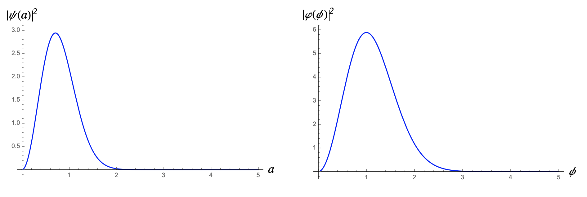
Figure 1: On the left hand side is the plot of $|\psi(a)|^{2}$ for $E=1$, and on the right hand side is the plot of $|\varphi(\phi)|^{2}$ for $m=1$ and $n=1$. We set $\lambda=1$, which is the value of the parameter in the GR limit.

4.2 Solution to the WDW equation in the limit $a\to 0$

Now we are interested in studying the case when the scale factor is small, or $a\to 0$. This means that we are in the early times of the cosmic evolution. Precisely for short distances HL theory is more appropriated than GR since it is well behaved in this limit and it should give sensible results near the singularity. In this scenario, the surviving terms in the gravitational part of equation (4) are the ones with HL parameters $g_{\text{r}}$ and $g_{\text{s}}$, as well as the one with the parameter $p$. When $a$ is small, we cannot neglect the quantum effects, which means that the operator ordering parameter $p$ becomes more significant.

In the matter fields part of equation (4), we consider that $\frac{1}{a^{2}}$ is smaller than $\frac{1}{a^{4}}$ when $a\to 0$, so we can neglect the former one. Therefore, in this limit, the higher-order terms dominate, and the WDW equation (4) reads

$$\bigg{\{}{\partial^{2}\over\partial a^{2}}+\frac{p}{a}{\partial\over\partial a}+\gamma\left(g_{\text{r}}+\frac{g_{\text{s}}}{a^{2}}\right)+2\sum_{n}\left[-{\partial^{2}\over\partial\phi^{2}_{n}}+\frac{1}{2}\frac{\gamma\beta_{3}}{a^{4}}\phi_{n}^{2}\right]\bigg{\}}\Psi=0.$$ (43)

In order to obtain solutions for this equation, we need to make the following change of variables for each $\phi_{n}$ [32]

$$\eta_{n}=\frac{\phi_{n}^{2}}{2a^{2}}.$$ (44)

With the change of coordinates $(a,\phi_{n})\to(a,\eta_{n})$, the WDW equation becomes

$$\left[a^{2}{\partial^{2}\over\partial a^{2}}+pa{\partial\over\partial a}+\gamma\left(a^{2}g_{\text{r}}+g_{\text{s}}\right)-2\sum_{n}\left(2\eta_{n}{\partial^{2}\over\partial\eta^{2}_{n}}+{\partial\over\partial\eta_{n}}-\gamma\beta_{3}\eta_{n}\right)\right]\Psi=0.$$ (45)

Hence, the change of coordinates introduced earlier makes the wave function separable:

$$\Psi(a,\eta_{n})=\psi(a)\varphi(\eta_{n}).$$ (46)

The WDW equation (43) separates into

$$\left(a^{2}{d^{2}\over da^{2}}+pa{d\over da}+\gamma\left(a^{2}g_{\text{r}}+g_{\text{s}}\right)+\chi\right)\psi(a)=0,$$ (47)

and

$$\sum_{n}\left(2\eta_{n}{d^{2}\over d\eta^{2}_{n}}+{d\over d\eta_{n}}-\gamma\beta_{3}\eta_{n}+\chi\right)\varphi(\eta_{n})=0.$$ (48)

The general solution of equation (47) is given by a linear combination of the Bessel functions and Neumann functions [45]

$$\psi(a)=C_{1}\,a^{\frac{1-p}{2}}\,J_{\nu}(a\sqrt{\gamma g_{\text{r}}})+C_{2}\,a^{\frac{1-p}{2}}Y_{\nu}(a\sqrt{\gamma g_{\text{r}}}),$$ (49)

where the order of the Bessel function is $\nu=\frac{1}{2}\sqrt{1+p(p-2)-4(\gamma g_{\text{s}}+\chi)}$, which depends on the value of the parameters $\lambda$ and $p$. As previously mentioned, $\lambda$ is a dynamical coupling constant which can take different values in the UV regime. Here, we will work with values $\lambda>1/3$ such that $(3\lambda-1)\neq 0$. Also, in order to avoid a complex argument in the Bessel functions, we will take $g_{\text{r}}>0$. The bounds for $p$ and $g_{\text{s}}$ will be given below.

Since we are considering the limit $a\to 0$, not both functions in the general solution (49) are admissible. This can be seen from the asymptotic forms of the Bessel and Neumann functions

$$J_{\nu}(z)\sim z^{\nu},\quad Y_{\nu}(z)\sim-z^{-\nu}.$$ (50)

Notice that the Neumann functions, $Y_{\nu}(z)$, diverge at the origin, so we set $C_{2}=0$, and keep only the asymptotic form of $J_{\nu}(z)$ for small $z$.

Therefore, for small $a$ the general solution (49) reads

$$\psi(a)\sim\,a^{\frac{1-p}{2}+\nu}.$$ (51)

This solution is indeed regular at $a=0$ satisfying the Hawking-Page boundary condition (b). However, one needs to be careful with the choice of operator ordering because for $p>1$ we have a divergence. Nevertheless, for $p<1$ the divergence is avoided, and the wormhole boundary condition is satisfied. As for $g_{\text{s}}$, we can restrict their value by demanding $\nu$ to be real. Hence, the bound for $g_{\text{s}}$ is

$$g_{\text{s}}<\frac{1+p(p-2)}{4\gamma}-\frac{\chi}{\gamma}.$$ (52)

In Figure 2, we show the plot of the solution of the gravitational part (49) for $C_{2}=0$. We choose three different values of $\lambda$. The plot 2 shows that the higher the value of the parameter $\lambda$, the higher the frequency of oscillation of $\psi(a)$ for $a$ far away from the origin. It is also observed that the amplitude decreases as $\lambda$ grows. This does not contradict the Hawking-Page boundary conditions because we are interested in the behavior of the wave function for small $a$, and in that region, the solution is indeed regular, i.e. $\psi(a)=0$ for $a=0$.

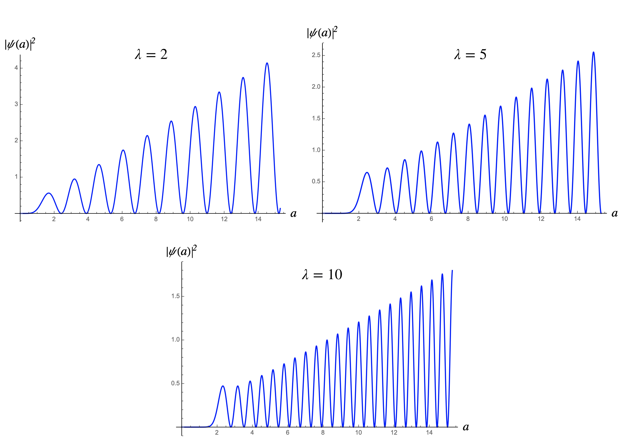
Figure 2: Plot of the square of the wave function, $\psi(a)\simeq a^{\frac{1-p}{2}}\,J_{\nu}(a\sqrt{\gamma g_{\text{r}}})$, for $p=-1$, $g_{\text{r}}=1$, $g_{\text{s}}=-1$, and for three different values of the parameter $\lambda$.

We still need to give the allowed values of $\chi$. This will arise naturally as we explore the solution of equation (48).

Equation (48) is a Hermite-like equation, hence its solution can be written as

$$\varphi_{m}(\eta_{n})=A_{m}\prod_{n}e^{-\frac{\rho}{2}\eta_{n}}H_{m_{n}}(\sqrt{\rho\eta_{n}}),$$ (53)

where $\chi=\rho(m+\frac{1}{2})$ for $m=0,1,2,\dots$, $\rho^{2}=\gamma\beta_{3}$, and $A_{m}=(2^{m}m!)^{-\frac{1}{2}}$ is the normalization constant.

Asymptotically, the solution behaves like

$$\varphi(\eta)\sim e^{-\frac{\rho}{2}\eta},$$ (54)

which implies that as $\eta\to\infty$ ($a\to 0$) the solution is regular.

In Figure 3, the solution (53) is plotted considering one scalar particle ($m=1$) in the first excited state ($n=1$) for different values of the parameter $\lambda$. As we can see, for higher values of the parameter $\lambda$, the peak of the distribution becomes narrower.

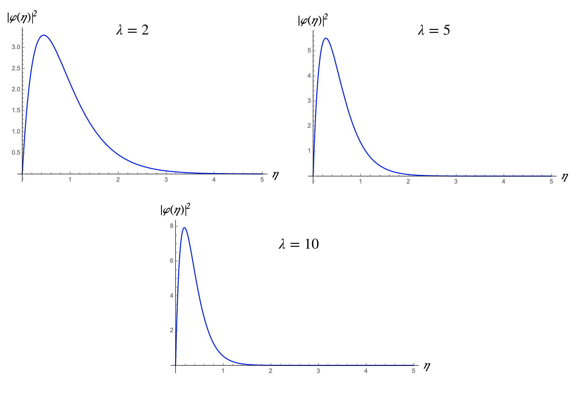
Figure 3: Plot of the square of the wave function, $\varphi_{1}(\eta)\simeq e^{-\frac{\rho}{2}\eta}H_{1}(\sqrt{\rho\eta})$, for $n=1$, $m=1$ and for three different values of the parameter $\lambda$.

Finally, the full wave function in this limit behaves like

$$\Psi(a,\eta)\sim a^{\frac{1-p}{2}+\nu}\,e^{-\frac{\rho}{2}\eta}.$$ (55)

which is of course regular near the origin, obeying the Hawking-Page boundary condition (b).

It is worth mentioning that this solution resembles the one found when a massive scalar field is minimally coupled to gravity [32].

The solutions here presented were obtained for zero cosmological constant, but they can be extended for $\Lambda\neq 0$.

4.3 Solution to WDW equation for $\Lambda\neq 0$

Solutions to the WDW equation in the context of a FLRW minisuperspace model have been studied in [8] considering all the possible values of the cosmological constant. Here we will analyze some of the results in the context of wormhole solutions.

$\bullet$ Solution for $\Lambda>0$

In the limit $a\to\infty$, the term with $a^{2}$ is smaller compared to the term with $a^{4}$, so we only keep the latter. Also, the operator ordering parameter $p$ is no longer significant, and we end up with the following equations:

$$\left({\partial^{2}\over\partial a^{2}}+g_{\Lambda}a^{4}\right)\psi(a)=0$$ (56)

and

$$\sum_{n}\left(-{\partial^{2}\over\partial\phi^{2}_{n}}+\omega_{1}^{2}\phi_{n}^{2}\right)\varphi(\phi_{n})=0,$$ (57)

where $g_{\Lambda}=\frac{2\gamma\Lambda}{3}$, and the separation constant has been set to zero so that we can obtain physically meaningful solutions.

The solution to Eq. (56) is given by a combination of Bessel and Neumann functions

$$\psi(a)=\overline{C}_{1}\sqrt{a}\,J_{1/6}\left(\frac{\sqrt{g_{\Lambda}}}{3}a^{3}\right)+\overline{C}_{2}\sqrt{a}\,Y_{1/6}\left(\frac{\sqrt{g_{\Lambda}}}{3}a^{3}\right),$$ (58)

while the solution of (57) is given in terms of Hermite functions, and it is the same as in (41).

The behavior of (58) for large arguments is oscillatory. This can be easily seen by making use of the asymptotic expansion for Bessel and Neumann functions for $|z|\rightarrow\infty$

$$J_{\nu}(z)\sim\sqrt{\frac{2}{\pi z}}\cos\left(z-\frac{\nu\pi}{2}-\frac{\pi}{4}\right),$$

$$N_{\nu}(z)\sim\sqrt{\frac{2}{\pi z}}\sin\left(z-\frac{\nu\pi}{2}-\frac{\pi}{4}\right).$$ (59)

Hence, using these expressions, the asymptotic behavior of $\psi(a)$ for large $a$ reads

$$\psi(a)\sim\frac{C_{1}}{a}\cos\left(\frac{\sqrt{g_{\Lambda}}}{3}a^{3}-\frac{\pi}{12}-\frac{\pi}{4}\right)+\frac{C_{2}}{a}\sin\left(\frac{\sqrt{g_{\Lambda}}}{3}a^{3}-\frac{\pi}{12}-\frac{\pi}{4}\right),$$ (60)

where $C_{i}=\overline{C}_{i}\sqrt{6/\pi\sqrt{g_{\Lambda}}}$, for $i=1,2$.

As we can see in Figure 4, $\psi(a)$ has an oscillatory behavior for large $a$. Even if we take into account the solution of the matter part (which goes like $\exp(-\phi^{2})$), the oscillatory behavior will not be suppressed. Hence, the total wave function $\Psi(a,\phi)$, for large $a$, does not satisfy the required boundary condition, and for that reason it does not describe a quantum wormhole. However, we may interpret this wave function as a Lorentzian or Friedmann Universe.

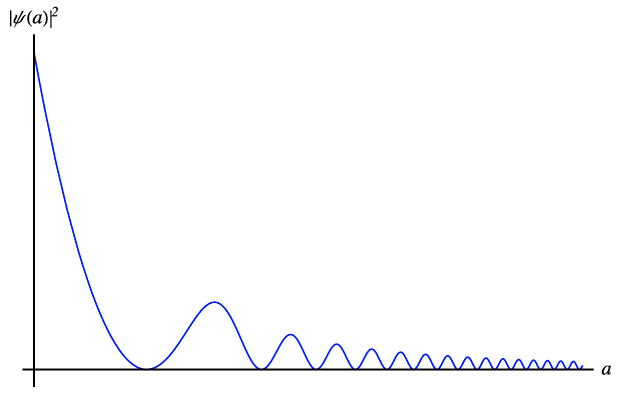
Figure 4: Qualitative plot of $|\psi(a)|^{2}$ for $\lambda=1$, which is the value that the parameter takes in the GR limit. The wave function $\psi(a)$ oscillates for large $a$.

In the limit $a\to 0$ we are back in the HL regime, where the cosmological constant is no longer significant. Indeed, the solutions in that limit will behave like in equation (55), and satisfy the wormhole boundary condition (b).

From the above analysis, we see that the presence of a positive cosmological constant makes the wave function of the Universe to have an oscillatory behavior in the limit $a\to\infty$. For that reason, the Hawking-Page wormholes cannot exist in this scenario.

$\bullet$ Solution for $\Lambda<0$

For $a\to\infty$, and $g_{\Lambda}<0$ the equations to solve are

$$\left({\partial^{2}\over\partial a^{2}}-(-g_{\Lambda})a^{4}\right)\psi(a)=0,$$ (61)

and

$$\sum_{n}\left(-{\partial^{2}\over\partial\phi^{2}_{n}}+\omega_{1}^{2}\phi_{n}^{2}\right)\varphi(\phi_{n})=0.$$ (62)

The solution of the gravitational part (61) is a combination of the modified Bessel functions, that is

$$\psi(a)=C_{1}\sqrt{a}\,I_{1/6}\left(\frac{\sqrt{-g_{\Lambda}}}{3}a^{3}\right)+C_{2}\sqrt{a}\,K_{1/6}\left(\frac{\sqrt{-g_{\Lambda}}}{3}a^{3}\right),$$ (63)

while the solution of (62) is again given in terms of the Hermite functions, and it is the same as in (41).

Now, let us write the asymptotic form of the modified Bessel functions for large argument ($|z|\to\infty$)

$$I_{\nu}(z)\sim\frac{e^{z}}{\sqrt{2\pi z}},\quad K_{\nu}(z)\sim\sqrt{\frac{\pi}{2z}}e^{-z}.$$ (64)

From these expressions we notice that $I_{\nu}(z)$ grows exponentially as $z\to\infty$, hence we only keep $K_{\nu}(z)$ because it decays exponentially for large $z$ and satisfies the wormhole boundary condition (a).

Therefore, the asymptotic solution of (61) is

$$\psi(a)\sim\frac{1}{a}\,e^{(-\sqrt{-g_{\Lambda}}/3)a^{3}}.$$ (65)

The plot of this solution is shown in Figure 5. We see that for large $a$, the wave function is exponentially damped, however it is highly suppressed due to the factor $e^{-a^{3}}$. The full wave function in this limit is

$$\Psi(a,\phi)\sim\frac{1}{a}\,e^{(-\sqrt{-g_{\Lambda}}/3)a^{3}}e^{-\frac{\phi^{2}}{2}\omega_{1}}.$$ (66)

It seems that in the limit of large $a$, we have a exponentially damped wave function. Indeed, this solution satisfies the Hawking-Page boundary condition (a).

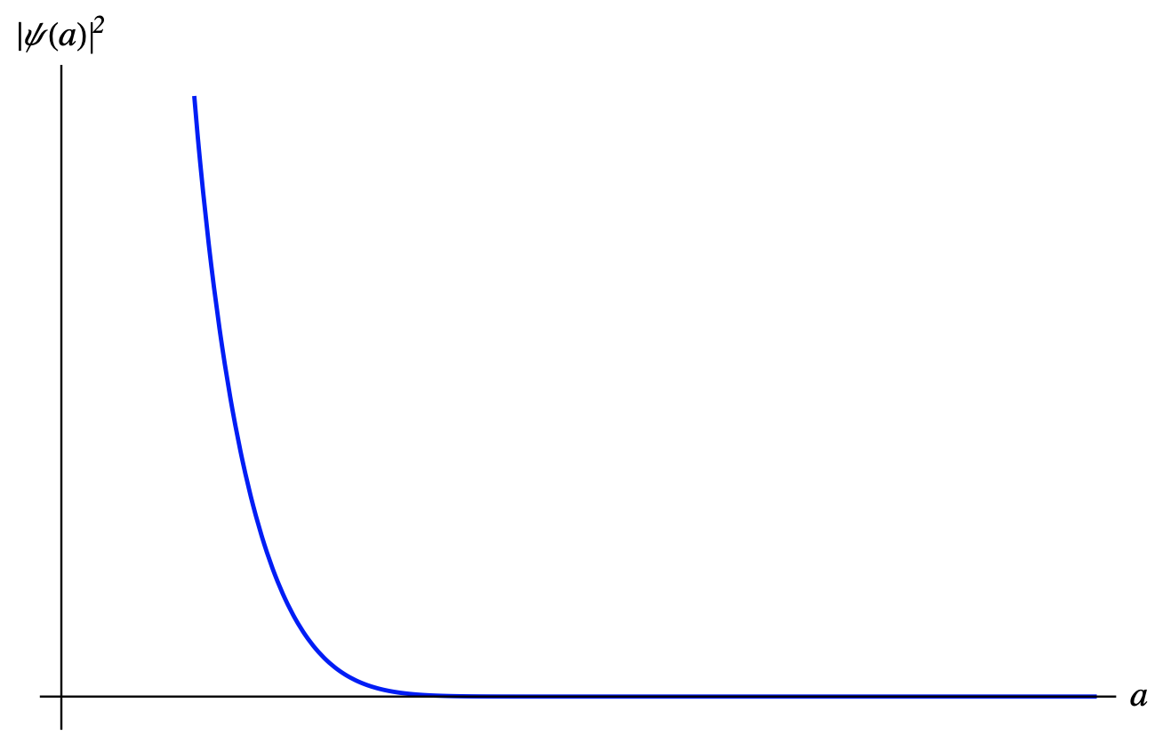
Figure 5: Qualitative plot of $|\psi(a)|^{2}$ for $\lambda=1$. The wave function $\psi(a)$ is exponentially damped for large $a$, but it is also highly suppressed.

On the other hand, in the region of the early Universe, that is, in the limit $a\to 0$, the HL terms are the ones that dominate, and the cosmological constant does not appear. Hence, we are back to the case with solution (55), which agrees with the wormhole boundary condition (b).

The performed analysis shows that for a negative cosmological constant we have a exponentially (but highly suppressed) damped behavior in the limit $a\to\infty$, and a regular behavior in the limit $a\to 0$. This satisfies both Hawking-Page boundary conditions. Hence, in a Universe with negative cosmological constant, wormhole configurations may exist.

5 Final remarks

We have studied Euclidean quantum wormholes in the context of the projectable version of the HL gravity. We considered a FLRW closed Universe minisuperspace model coupled to a scalar field, which we treated as a perturbation, which is expanding on hyperspherical harmonics on the 3-sphere. We obtained a WDW equation by canonically quantizing such model. As expected, the gravitational part of the WDW equation is fully characterized by the scale factor. On the other hand, in the matter part of the equation, the coefficients of the scalar harmonics and the scale factor appear. This is a consequence of the higher-order spatial derivative terms in the matter action. In order to obtain analytical solutions to the full WDW equation (gravity$+$matter) we solved it by considering limiting cases of small and large scale factor.

In the limit of the very late Universe (large scale factor) and considering a vanishing cosmological constant, the resulting WDW equation turned out to be a sum of two harmonic oscillator equations, one for the matter fields and one for the scale factor. The WDW equation is similar to the one found in GR when considering a model of gravity coupled to a conformally invariant scalar field as shown by Hawking [20]. In this case, the solution of the WDW equation is a product of two harmonic oscillator wave functions, which are given in terms of Hermite polynomials. This solution is exponentially damped at large values of the radius $a$ agreeing with the Hawking-Page boundary condition (a). It is also important to point out that this case corresponds to the Hamiltonian constraint in GR, where the additional scalar degree of freedom of the projectable theory is not evident.

In the limit of the very early Universe (small scale factor) things get more interesting because the quantum effects cannot be neglected, and the operator ordering parameter $p$ becomes more significant. In this regime, the HL terms dominate, and hence the cosmological constant term can be neglected. The WDW equation turned out to be non-separable because the term $\frac{\phi^{2}}{a^{4}}$ appeared in the matter part. However, we avoided this problem by using a suitable choice of coordinates. Fortunately, the equations obtained after this change have known solutions. Specifically, the equation of the gravitational part is a Bessel-like equation, thus their solutions are a linear combination of Bessel functions of the first and second kind. We kept the function $J_{\nu}(z)$ because it is the one that satisfies the wormhole boundary condition (b), that is, it is regular in the limit of small values of the scale factor. However, as the value of $a$ increases we start to see an oscillatory behavior. This does not contradict the Hawking-Page conjecture, it just means that $\psi(a)$ is regular in a different way.

The matter equation is given in terms of the new coordinate $\eta=\frac{\phi^{2}}{2a^{2}}$, and also has known solutions, namely, Hermite polynomials. Notice that at small values of the radius $a$, $\eta\to\infty$. In this limit, the solution behaves like $\varphi(\eta)\sim e^{-\frac{\rho}{2}\eta}$. Therefore, it eventually goes to zero, and hence is also regular, which agrees with the Hawking-Page boundary condition (b).

The solution obtained in the limit of small radius $a$ is similar to the one obtained when a massive scalar field is minimally coupled to Einstein’s gravity. This observation is interesting because it means that the HL gravity terms naturally behave like some kind of ’effective mass’.

We also gave different values of the running parameter $\lambda$ of HL theory in the limit $a\to 0$. The effect of $\lambda$ on $\psi(a)$ was decrease the amplitude. It is also observed the increment on the frequency of oscillation, but it remained regular at the origin, which is the region we are interested in. On the other hand, its effect on $\varphi(\eta)$ was to make the function more localized or peaked.

Supposedly, a necessary condition for wormhole-like solutions to appear is to take $\Lambda=0$. However, we expanded our analysis by considering the case of nonzero cosmological constant, which dominates in the IR limit. As expected, for $\Lambda>0$ we found oscillatory solutions, indeed, this happens because we are in a classically allowed region, i.e. the WDW potential $V(a)<0$. Thus, this solution does not satisfy the wormhole boundary condition (a) meaning that wormholes cannot exist in this scenario. For $\Lambda<0$ we obtained a damped solution. This is also not surprising because it just means that we are in a classically forbidden region, $V(a)>0$. This solution combined with the one found in the limit $a\to 0$ tell us that wormholes might exist in a Universe with negative cosmological constant.

Finally we want to mention that stable Euclidean wormhole solutions do exist in Anti-de Sitter spacetime via the holographic correspondence [46, 47]. It would be interesting to find a relation between these issues and the result presented in our paper. In addition for future work, it would be interesting, to look for numerical solutions for the full equation (4) and analyze in detail and interpret physically these solutions.

Acknowledgments

A.Vazquez would like to thank CONACyT for a grant.

References

- [1] P. Hoava, “Quantum Gravity at a Lifshitz Point,” Phys. Rev. D 79, 084008 (2009) doi:10.1103/PhysRevD.79.084008 [arXiv:0901.3775 [hep-th]].
- [2] S. Weinfurtner, T. P. Sotiriou and M. Visser, “Projectable Hoava-Lifshitz gravity in a nutshell,” J. Phys. Conf. Ser. 222, 012054 (2010) doi:10.1088/1742-6596/222/1/012054 [arXiv:1002.0308 [gr-qc]].
- [3] T. P. Sotiriou, “Hoava-Lifshitz gravity: a status report,” J. Phys. Conf. Ser. 283, 012034 (2011) doi:10.1088/1742-6596/283/1/012034 [arXiv:1010.3218 [hep-th]].
- [4] A. Wang, “Hoava gravity at a Lifshitz point: A progress report,” Int. J. Mod. Phys. D 26, no. 07, 1730014 (2017) doi:10.1142/S0218271817300142 [arXiv:1701.06087 [gr-qc]].
- [5] S. Mukohyama, “Hoava-Lifshitz Cosmology: A Review,” Class. Quant. Grav. 27, 223101 (2010) doi:10.1088/0264-9381/27/22/223101 [arXiv:1007.5199 [hep-th]].
- [6] K. Izumi and S. Mukohyama, “Nonlinear superhorizon perturbations in Hoava-Lifshitz gravity,” Phys. Rev. D 84, 064025 (2011) doi:10.1103/PhysRevD.84.064025 [arXiv:1105.0246 [hep-th]].
- [7] A. E. Gumrukcuoglu, S. Mukohyama and A. Wang, “General relativity limit of Hoava-Lifshitz gravity with a scalar field in gradient expansion,” Phys. Rev. D 85, 064042 (2012) doi:10.1103/PhysRevD.85.064042 [arXiv:1109.2609 [hep-th]].
- [8] O. Bertolami and C. A. D. Zarro, “Hoava-Lifshitz Quantum Cosmology,” Phys. Rev. D 84, 044042 (2011) [arXiv:1106.0126 [hep-th]].
- [9] T. Christodoulakis and N. Dimakis, “Classical and Quantum Bianchi Type III vacuum Hoava-Lifshitz Cosmology,” J. Geom. Phys. 62, 2401 (2012) [arXiv:1112.0903 [gr-qc]].
- [10] J. P. M. Pitelli and A. Saa, “Quantum Singularities in Hoava-Lifshitz Cosmology,” Phys. Rev. D 86, 063506 (2012) [arXiv:1204.4924 [gr-qc]].
- [11] B. Vakili and V. Kord, “Classical and quantum Hořava-Lifshitz cosmology in a minisuperspace perspective,” Gen. Rel. Grav. 45, 1313 (2013) doi:10.1007/s10714-013-1527-8 [arXiv:1301.0809 [gr-qc]].
- [12] O. Obregón and J. A. Preciado, “Quantum cosmology in Hoava-Lifshitz gravity,” Phys. Rev. D 86, 063502 (2012) [arXiv:1305.6950 [gr-qc]].
- [13] D. Benedetti and J. Henson, “Spacetime condensation in (2+1)-dimensional CDT from a Hoava-Lifshitz minisuperspace model,” Class. Quantum Grav. 32, 215007 (2015) [arXiv:1410.0845 [gr-qc]].
- [14] R. Cordero, H. Garcia-Compean and F. J. Turrubiates, “A phase space description of the FLRW quantum cosmology in Hoava-Lifshitz type gravity,” Gen. Rel. Grav. 51, no. 10, 138 (2019) doi:10.1007/s10714-019-2627-x [arXiv:1711.04933 [gr-qc]].
- [15] J. A. Wheeler, “Geons,” Phys. Rev. 97, 511 (1955). doi:10.1103/PhysRev.97.511
- [16] A. Anderson and B. S. DeWitt, “Does the Topology of Space Fluctuate?,” Found. Phys. 16, 91 (1986). doi:10.1007/BF01889374
- [17] G. W. Gibbons and S. W. Hawking, “Euclidean quantum gravity,” Singapore, Singapore: World Scientific (1993) 586 p
- [18] S. B. Giddings and A. Strominger, “Axion Induced Topology Change in Quantum Gravity and String Theory,” Nucl. Phys. B 306, 890 (1988). doi:10.1016/0550-3213(88)90446-4
- [19] S. R. Coleman, “Why There Is Nothing Rather Than Something: A Theory of the Cosmological Constant,” Nucl. Phys. B 310, 643 (1988). doi:10.1016/0550-3213(88)90097-1
- [20] S. W. Hawking, “Baby Universes 2,” Mod. Phys. Lett. A 5, 453 (1990). doi:10.1142/S0217732390000524
- [21] A. Hebecker, T. Mikhail and P. Soler, “Euclidean wormholes, baby Universes, and their impact on particle physics and cosmology,” Front. Astron. Space Sci. 5, 35 (2018) doi:10.3389/fspas.2018.00035 [arXiv:1807.00824 [hep-th]].
- [22] A. Hebecker, P. Mangat, S. Theisen and L. T. Witkowski, “Can Gravitational Instantons Really Constrain Axion Inflation?,” JHEP 1702, 097 (2017) doi:10.1007/JHEP02(2017)097 [arXiv:1607.06814 [hep-th]].
- [23] S. W. Hawking and D. N. Page, “The spectrum of wormholes,” Phys. Rev. D 42, 2655 (1990). doi:10.1103/PhysRevD.42.2655
- [24] R. L. Arnowitt, S. Deser and C. W. Misner, “The dynamics of general relativity,” Gen. Rel. Grav. 40, 1997 (2008) doi:10.1007/s10714-008-0661-1 [gr-qc/0405109].
- [25] J. J. Halliwell, “Introductory Lectures On Quantum Cosmology,” arXiv:0909.2566 [gr-qc].
- [26] D. L. Wiltshire, “An introduction to quantum cosmology,” gr-qc/0101003.
- [27] M. Botta-Cantcheff, N. Grandi and M. Sturla, “Wormhole solutions to Horava gravity,” Phys. Rev. D 82, 124034 (2010) doi:10.1103/PhysRevD.82.124034 [arXiv:0906.0582 [hep-th]].
- [28] E. J. Son and W. Kim, “Traversable wormhole in the deformed Hořava-Lifshitz gravity,” Phys. Rev. D 83, 124012 (2011) doi:10.1103/PhysRevD.83.124012 [arXiv:1011.3596 [gr-qc]].
- [29] J. Bellorin, A. Restuccia and A. Sotomayor, “Wormholes and naked singularities in the complete Hoava theory,” Phys. Rev. D 90, no. 4, 044009 (2014) doi:10.1103/PhysRevD.90.044009 [arXiv:1404.2884 [gr-qc]].
- [30] J. Bellor n, A. Restuccia and A. Sotomayor, “Solutions with throats in Horava gravity with cosmological constant,” Int. J. Mod. Phys. D 25, no. 02, 1650016 (2015) doi:10.1142/S0218271816500164 [arXiv:1501.04568 [gr-qc]].
- [31] S. Ruz, S. Debnath, A. K. Sanyal and B. Modak, “Euclidean wormholes with minimally coupled scalar fields,” Class. Quant. Grav. 30, 175013 (2013) doi:10.1088/0264-9381/30/17/175013 [arXiv:1308.0232 [gr-qc]].
- [32] D.M. Solomons, The wave function of the Universe, Ph.D. Thesis, University of Cape Twon, 1993.
- [33] A. Carlini, D. H. Coule and D. M. Solomons, “Classical and quantum wormholes with perfect fluids and scalar fields,” Mod. Phys. Lett. A 11, 1453 (1996). doi:10.1142/S0217732396001454
- [34] A. Carlini, D. H. Coule and D. M. Solomons, “Euclidean quantum wormholes with scalar fields,” Int. J. Mod. Phys. A 12, 3517 (1997). doi:10.1142/S0217751X97001821
- [35] H. Kim, “Axionic wormholes: More on their classical and quantum aspects,” Nucl. Phys. B 527, 311 (1998) doi:10.1016/S0550-3213(98)00397-6 [hep-th/9706015].
- [36] E. Kiritsis and G. Kofinas, “Hoava-Lifshitz Cosmology,” Nucl. Phys. B 821, 467 (2009) doi:10.1016/j.nuclphysb.2009.05.005 [arXiv:0904.1334 [hep-th]].
- [37] G. Calcagni, “Cosmology of the Lifshitz Universe,” JHEP 0909, 112 (2009) doi:10.1088/1126-6708/2009/09/112 [arXiv:0904.0829 [hep-th]].
- [38] A. N. Tawfik, A. M. Diab and E. A. El Dahab, “Friedmann inflation in Hoava-Lifshitz gravity with a scalar field,” Int. J. Mod. Phys. A 31, no. 09, 1650042 (2016) doi:10.1142/S0217751X16500421 [arXiv:1603.09667 [gr-qc]].
- [39] S. Mukohyama, “Scale-invariant cosmological perturbations from Hoava-Lifshitz gravity without inflation,” JCAP 0906, 001 (2009) doi:10.1088/1475-7516/2009/06/001 [arXiv:0904.2190 [hep-th]].
- [40] T. Fujimori, T. Inami, K. Izumi and T. Kitamura, “Power-counting and Renormalizability in Lifshitz Scalar Theory,” Phys. Rev. D 91, no. 12, 125007 (2015) doi:10.1103/PhysRevD.91.125007 [arXiv:1502.01820 [hep-th]].
- [41] S. W. Hawking, “Baby Universes,” Mod. Phys. Lett. A 5, 145-155 (1990).
- [42] S. W. Hawking, “Wormholes in Spacetime,” Phys. Rev. D 37, 904 (1988). doi:10.1103/PhysRevD.37.904
- [43] L. Lindblom, N. W. Taylor and F. Zhang, “Scalar, Vector and Tensor Harmonics on the Three-Sphere,” Gen. Rel. Grav. 49, no. 11, 139 (2017) doi:10.1007/s10714-017-2303-y [arXiv:1709.08020 [gr-qc]].
- [44] R. Steigl and F. Hinterleitner, “Factor ordering in standard quantum cosmology,” Class. Quant. Grav. 23, 3879 (2006) doi:10.1088/0264-9381/23/11/013 [gr-qc/0511149].
- [45] W.W. Bell, Special functions for scientists and engineers, Dover Publications, 2004.
- [46] J. M. Maldacena and L. Maoz, “Wormholes in AdS,” JHEP 0402, 053 (2004) doi:10.1088/1126-6708/2004/02/053 [hep-th/0401024].
- [47] P. Betzios, E. Kiritsis and O. Papadoulaki, “Euclidean Wormholes and Holography,” JHEP 1906, 042 (2019) doi:10.1007/JHEP06(2019)042 [arXiv:1903.05658 [hep-th]].