Supervised Learning: No Loss No Cry

Abstract

Supervised learning requires the specification of a loss function to minimise. While the theory of admissible losses from both a computational and statistical perspective is well-developed, these offer a panoply of different choices. In practice, this choice is typically made in an ad hoc manner. In hopes of making this procedure more principled, the problem of learning the loss function for a downstream task (e.g., classification) has garnered recent interest. However, works in this area have been generally empirical in nature.

In this paper, we revisit the SLIsotron algorithm of Kakade et al. (2011) through a novel lens, derive a generalisation based on Bregman divergences, and show how it provides a principled procedure for learning the loss. In detail, we cast SLIsotron as learning a loss from a family of composite square losses. By interpreting this through the lens of proper losses, we derive a generalisation of SLIsotron based on Bregman divergences. The resulting BregmanTron algorithm jointly learns the loss along with the classifier. It comes equipped with a simple guarantee of convergence for the loss it learns, and its set of possible outputs comes with a guarantee of agnostic approximability of Bayes rule. Experiments indicate that the BregmanTron substantially outperforms the SLIsotron, and that the loss it learns can be minimized by other algorithms for different tasks, thereby opening the interesting problem of loss transfer between domains.

1 Introduction

Computationally efficient supervised learning essentially started with the PAC framework of Valiant (1984), in which the goal was to learn in polynomial time a function being able to predict a label (or class, among two possible) for i.i.d. inputs. The initial loss, whose minimization enforces the accurate prediction of labels, was the binary zero-one loss which returns 1 iff a mistake is made.

The zero-one loss was later progressively replaced in learning algorithms for tractability reasons, including its non-differentiability and the structural complexity of its minimization (Kearns & Vazirani, 1994; Auer et al., 1995). From the late nineties, a zoo of losses started to be used for tractable machine learning (ML), the most popular ones built from the square loss and the logistic loss. Recently, there has been a significant push to widen even more the choice of loss; to pick a few, see Grabocka et al. (2019); Kakade et al. (2011); Liu et al. (2019); Mei & Moura (2018); Nock & Nielsen (2008, 2009); Reid & Williamson (2010); Siahkamari et al. (2019); Streeter (2019); Sypherd et al. (2019).

Seldom do such works ground reasons for change of the loss outside of tractability at large. It turns out that statistics and Bayes decision theory give a precise reason, one which has long been the object of philosophical and formal debates (de Finetti, 1949). It starts from a simple principle:

Bayes rule is optimal for the loss at hand,

a property known as properness (Savage, 1971). Then comes a less known subtlety: a proper loss as commonly used for real-valued prediction, such as the square and logistic loss, involves an implicit canonical link (Reid & Williamson, 2010) function that maps class probabilities (such as the output of Bayes rule) to real values. This is exemplified by the sigmoid (inverse) link in deep learning.

Supervised learning in a Bayesian framework can thus be more broadly addressed by learning a classifier and a link for the domain at hand, which implies learning a proper canonical loss with the classifier. This loss, if suitably expressed, can be used for training. This kills two birds in one shot: we get access not just to real valued predictions, but also a way to embed them into class probability estimates via the inverse link: we directly learn to estimate Bayes rule.

A large number of papers, especially recently, have tried to push forward the problem of learning the loss, including e.g. Grabocka et al. (2019); Liu et al. (2019); Mei & Moura (2018); Siahkamari et al. (2019); Streeter (2019); Sypherd et al. (2019), but none of those dealing with supervised learning alludes to properness to ground the choice of the loss, therefore taking the risk of fitting a loss whose (unknown) optima may fail to contain Bayes rule. To the best of our knowledge, Nock & Nielsen (2008) is the first paper grounding the search of the loss within properness and Kakade et al. (2011) brings the first algorithm (SlIsotron) and associated theoretical results for fitting the link — though subject to restrictive assumptions on Bayes rule and on the target distribution, the risk to fit probabilities outside $[0,1]$, and finally falling short of showing convergence that would comply with the classical picture of ML, either for training or generalization.

Our major contribution is a new algorithm, the BregmanTron (Algorithm 2), a generalisation of the SlIsotron (Kakade et al., 2011) to learn proper canonical losses. BregmanTron exploits two dual views of proper losses, guarantees class probability estimates in $[0,1]$, and uses Lipschitz constraints that can be tuned at runtime.

Our formal contribution includes a simple convergence guarantee for this algorithm which alleviates all assumptions on the domain and Bayes rule in Kakade et al. (2011). Our result shows that convergence happens as a function of the discrepancy between our estimate and the true value of of the mean operator – a sufficient statistic for the class (Patrini et al., 2014). As the discrepancy converges to zero, the estimated (link, classifier) by the BregmanTron converges to a stable output. To come to this result, we pass through an intermediate step in which we show a particular explicit form for any differentiable proper composite loss, of a Bregman divergence (Bregman, 1967). All proofs are given in an appendix, denoted App.

2 Definitions and notations

The following shorthands are used: $[n]\stackrel{{\scriptstyle\mathrm{.}}}{{=}}\{1,2,...,n\}$ for $n\in\mathbb{N}_{*}$, for $z\geq 0,a\leq b\in\mathbb{R}$, denote $z\cdot[a,b]\stackrel{{\scriptstyle\mathrm{.}}}{{=}}[za,zb]$ and $z+[a,b]\stackrel{{\scriptstyle\mathrm{.}}}{{=}}[z+a,z+b]$. We also let $\overline{\mathbb{R}}\stackrel{{\scriptstyle\mathrm{.}}}{{=}}[-\infty,\infty]$. In (batch) supervised learning, one is given a training set of $m$ examples $S\stackrel{{\scriptstyle\mathrm{.}}}{{=}}\{({\bm{x}}_{i},y^{*}_{i}),i\in[m]\}$, where ${\bm{x}}_{i}\in{\mathcal{X}}$ is an observation (${\mathcal{X}}$ is called the domain: often, ${\mathcal{X}}\subseteq{\mathbb{R}}^{d}$) and $y^{*}_{i}\in\mathcal{Y}\stackrel{{\scriptstyle\mathrm{.}}}{{=}}\{-1,1\}$ is a label, or class. The objective is to learn a classifier $h:\mathcal{X}\rightarrow\mathbb{R}$ which belongs to a given set $\mathcal{H}$. The goodness of fit of some $h$ on ${S}$ is evaluated by a loss.

$\triangleright$ Losses: A loss for binary class probability estimation Buja et al. (2005) is some $\ell:\mathcal{Y}\times[0,1]\rightarrow\overline{\mathbb{R}}$ whose expression can be split according to partial losses $\ell_{1},\ell_{-1}$,

$$\ell(y^{*},u) \stackrel{{\scriptstyle\mathrm{.}}}{{=}} \llbracket y^{*}=1\rrbracket\cdot\ell_{1}(u)+\llbracket y^{*}=-1\rrbracket\cdot\ell_{-1}(u),$$ (1)

Its conditional Bayes risk function is the best achievable loss when labels are drawn with a particular positive base-rate,

$$\underline{L}(\pi) \stackrel{{\scriptstyle\mathrm{.}}}{{=}} \inf_{u}\mathsf{E}_{\mathsf{Y}\sim\pi}\ell(\mathsf{Y},u),$$ (2)

where $\Pr[\mathsf{Y}=1]=\pi$. A loss for class probability estimation $\ell$ is proper iff Bayes prediction locally achieves the minimum everywhere: $\underline{L}(\pi)=\mathsf{E}_{\mathsf{Y}}\ell(\mathsf{Y},\pi),\forall\pi\in[0,1]$, and strictly proper if Bayes is the unique minimum. Fitting a prediction $h(\bm{x})\in\mathbb{R}$ into some $u\in[0,1]$ as required in (1) is done via a link function.

$\triangleright$ Links, composite and canonical proper losses. A link $\psi:[0,1]\rightarrow\mathbb{R}$ allows to connect real valued prediction and class probability estimation. A loss can be augmented with a link to account for real valued prediction, $\ell_{\psi}(y^{*},z)\stackrel{{\scriptstyle\mathrm{.}}}{{=}}\ell(y^{*},\psi^{-1}(z))$ with $z\in\mathbb{R}$ (Reid & Williamson, 2010). There exists a particular link uniquely defined for any proper differentiable loss, the canonical link, as: $\psi\stackrel{{\scriptstyle\mathrm{.}}}{{=}}-\underline{L}^{\prime}$ (Reid & Williamson, 2010, Section 6.1). We note that the differentiability condition can be removed (Reid & Williamson, 2010, Footnote 6). As an example, for log-loss we find the link $\psi(u)=\log\frac{u}{1-u}$, with inverse the well-known sigmoid $\psi^{-1}(z)=({1+e^{-z}})^{-1}$. A canonical proper loss is a proper loss using the canonical link.

$\triangleright$ Convex surrogates. When the loss is proper canonical and symmetric ($\ell_{1}(u)=\ell_{-1}(1-u),\forall u\in(0,1)$), it was shown in Nock & Nielsen (2008, 2009) that there exists a convenient dual formulation amenable to direct minimization with real valued classifiers: a convex surrogate loss

$$F_{\ell}(z) \stackrel{{\scriptstyle\mathrm{.}}}{{=}} (-\underline{L})^{\star}(-z),$$ (3)

where $\star$ denotes the Legendre conjugate of $F$, $F^{\star}(z)\stackrel{{\scriptstyle\mathrm{.}}}{{=}}\sup_{z^{\prime}\in\mathrm{dom}(F)}\{zz^{\prime}-F(z^{\prime})\}$ (Boyd & Vandenberghe, 2004). For simplicity, we just call $F_{\ell}$ the convex surrogate of $\ell$. The logistic, square and Matsushita losses are all surrogates of proper canonical and symmetric losses. Such functions are called surrogates since they all define convenient upperbounds of the 0/1 loss. Any proper canonical and symmetric loss has $\ell(y^{*},z)\propto F_{\ell}(y^{*}z)$ so both dual forms are equivalent in terms of minimization Nock & Nielsen (2008, 2009).

$\triangleright$ Learning. Given a sample $S$, we learn $h$ by the empirical minimization of a proper loss on $S$ that we denote $\ell_{\psi}(S,h)\stackrel{{\scriptstyle\mathrm{.}}}{{=}}\mathbb{E}_{i}[\ell(y^{*}_{i},\psi^{-1}(h(\bm{x}_{i})))]$. We insist on the fact that minimizing any such loss does not just give access to a real valued predictor $h$: it also gives access to a class probability estimator given the loss (Nock & Nielsen, 2008, Section 5), Nock & Williamson (2019),

$$\Pr[\mathsf{Y}=1|\bm{x};h,\psi] \stackrel{{\scriptstyle\mathrm{.}}}{{=}} \psi^{-1}(h(\bm{x})),$$ (4)

so in the Bayesian framework, supervised learning can also encompass learning the link $\psi$ of the loss as well. If the loss is proper canonical, learning the link implies learning the loss. As usual, we assume $S$ sampled i.i.d. according to an unknown but fixed $\mathcal{D}$ and let $\ell_{.}(\mathcal{D},h)\stackrel{{\scriptstyle\mathrm{.}}}{{=}}\mathbb{E}_{S\sim\mathcal{D}}[\ell_{.}(S,h)]$.

3 Related work

Our problem of interest is learning not only a classifier, but also a loss function itself. A minimal requirement for the loss to be useful is that it is proper, i.e., it preserves the Bayes classification rule. Constraining our loss to this set ensures standard guarantees on the classification performance using this loss, e.g., using surrogate regret bounds.

Evidently, when choosing amongst losses, we must have a well-defined objective. We now reinterpret an algorithm of Kakade et al. (2011) as providing such an objective.

$\triangleright$ The SlIsotron algorithm. Kakade et al. (2011) considered the problem of learning a class-probability model of the form $\Pr(\mathsf{Y}=1\mid\bm{x})=u(\bm{w}_{*}^{\top}\bm{x})$ where $u(\cdot)$ is a 1-Lipschitz, non-decreasing function, and $\bm{w}_{*}\in\mathbb{R}^{d}$ is a fixed vector. They proposed SlIsotron, an iterative algorithm that alternates between gradient steps to estimate $\bm{w}_{*}$, and nonparametric isotonic regression steps to estimate $u$. SlIsotron provably bounds the expected square loss, i.e.,

$$\ell^{\mbox{\tiny{{sq}}}}_{\psi}(S,h) = \mathbb{E}_{\bm{x}\sim S}\left[\mathbb{E}_{y^{*}\sim S}[(y-\psi^{-1}(h(\bm{x})))^{2}|\bm{x}]\right],$$ (5)

where $h(\bm{x})=\bm{w}^{\top}\bm{x}$ is a linear scorer and $y\stackrel{{\scriptstyle\mathrm{.}}}{{=}}(y^{*}+1)/2$. The square loss has $2\cdot\ell^{\mbox{\tiny{{sq}}}}_{1}(u)\stackrel{{\scriptstyle\mathrm{.}}}{{=}}(1-u)^{2}$, $2\cdot\ell^{\mbox{\tiny{{sq}}}}_{-1}(u)\stackrel{{\scriptstyle\mathrm{.}}}{{=}}u^{2}$ , and conditional Bayes risk $2\cdot{\underline{L}^{\mbox{\tiny{{sq}}}}}(u)\stackrel{{\scriptstyle\mathrm{.}}}{{=}}u(1-u)$.

Observe now that the SlIsotron algorithm can be interpreted as follows: we jointly learn a classifier $h\in\mathcal{H}$ and composite link $\psi$ for the square loss $\ell\in\mathcal{L}$, as

$$\mathcal{L}\stackrel{{\scriptstyle\mathrm{.}}}{{=}}\{(y,z)\mapsto(y-\psi^{-1}(z))^{2}\colon\psi\text{ is 1-Lipschitz, invertible}\}.$$

That is, SlIsotron can be interpreted as finding a classifier and a link via all compositions of the square loss with a 1-Lipschitz, invertible function. Kakade et al. (2011) in fact do not directly analyze (5) but a lowerbound that directly follows from Jensen’s inequality:

$$\ell^{\mbox{\tiny{{sq}}}}_{\psi}(S,h) = \mathbb{E}_{\bm{x}\sim S}\left[\mathbb{E}_{y^{*}\sim S}[(y-\psi^{-1}(h(\bm{x})))^{2}|\bm{x}]\right],$$ (6)

$$\geq \mathbb{E}_{\bm{x}\sim S}\left[(\mathbb{E}_{y\sim S}[y|\bm{x}]-\psi^{-1}\circ h(\bm{x}))^{2}\right].$$

This does not change the problem as the slack is the expected (per observation) variance of labels in the sample, a constant given $S$. We shall return to this point in the sequel.

Kakade et al. (2011) make an assumption about Bayes rule, $\mathbb{E}_{y^{*}\sim\mathcal{D}}[y|\bm{x}]=\psi_{\mbox{\tiny{{opt}}}}^{-1}(\bm{w}_{\mbox{\tiny{{opt}}}}^{\top}\bm{x})$ with $\psi_{\mbox{\tiny{{opt}}}}^{-1}$ Lipschitz and $\|\bm{w}_{\mbox{\tiny{{opt}}}}\|\leq R$. Under such an assumption, it is shown that there exists an iteration $t=O((Rm/d)^{1/3})$ of the SlIsotron with $\max\{\tilde{\ell^{\mbox{\tiny{{sq}}}}}_{\psi}(S,h),\tilde{\ell^{\mbox{\tiny{{sq}}}}}_{\psi}(\mathcal{D},h)\}\leq\tilde{O}((dR^{2}/m)^{1/3})$ with high probability. Nothing is guaranteed outside this unknown "hitting" point, which we partially attribute to the lack of convergence results on training. Another potential downside from the Bayesian standpoint is that the estimates learned are not guaranteed to be in $[0,1]$ by the isotonic regression as modeled.

Algorithm 0 SlIsotron
Input: sample $S=\{(\bm{x}_{i},y_{i}),i=1,2,...,m\}$, iterations $T\in\mathbb{N}_{*}$. For $t=0,1,...,T-1$ [Step 1] If $t=0$ Then $\bm{w}_{t+1}=\bm{w}_{1}=\bm{0}$ Else fit $\bm{w}_{t+1}$ using $\displaystyle\bm{w}_{t+1}$ $\displaystyle=$ $\displaystyle\bm{w}_{t}-\frac{1}{m}\sum_{i=1}^{m}(u_{t}(\bm{x}_{i})-y_{i})\cdot\bm{x}_{i}$ (7) [Step 2] order indexes in $S$ so that $\bm{w}_{t+1}^{\top}\bm{x}_{i+1}\geq\bm{w}_{t+1}^{\top}\bm{x}_{i},\forall i\in[m-1]$; [Step 3] let $\bm{z}_{t+1}\stackrel{{\scriptstyle\mathrm{.}}}{{=}}\bm{w}_{t+1}^{\top}\bm{x}_{i+1}$ [Step 4] fit next link $\displaystyle u_{t+1}$ $\displaystyle\leftarrow$ $\displaystyle\sc{\rm IsotonicReg}(\hat{\bm{z}}_{t+1},S);\mbox{ \hskip 31.2982pt//fitting of $u_{t+1}$ given $\bm{z}_{t+1}$}$ (8) Output: $u_{T},\bm{w}_{T}$.

Figure 1: The SlIsotron algorithm of Kakade et al. (2011).

$\triangleright$ Learning the loss. Over the last decade, the problem of learning the loss has seen a considerable push for a variety of reasons: Sypherd et al. (2019) introduced a family of tunable losses, a subset of which being proper, aimed at increasing robustness in classification. Mei & Moura (2018) formulated the generalized linear model using Bregman divergences, though no relationship with proper losses is made, the loss function used integrates several regularizers breaking properness, the formal results rely on several quite restrictive assumptions and the guarantees can be quite loose if the true composite link comes from a loss that is not strongly convex "enough". In Streeter (2019), the problem studied is in fact learning the regularized part of the logistic loss, with no approximation guarantee. In Grabocka et al. (2019), the goal is to learn a loss defined by a neural network, without reference to proper losses and no approximation guarantee. Such a line of work also appears in a slightly different form in Liu et al. (2019). In Siahkamari et al. (2019), the loss considered is mainly used for metric learning, but integrates Bregman divergences. No mention of properness is made. Perhaps the most restrictive part of the approach is that it fits piecewise linear divergences, which are therefore not differentiable nor strictly convex.

Interestingly, none of these recent references alludes to properness to constrain the choice of the loss. Only the modelling of Mei & Moura (2018) can be related to properness via Theorem 1 proven below. The problem of learning the loss was introduced as loss tuning in Nock & Nielsen (2008) (see also Reid & Williamson (2010)). Though a general boosting result was shown for any tuned loss following a particular construction on its Bayes risk, it was restricted to losses defined from a convex combination of a basis set and no insight on improved convergence rates was given.

4 Learning proper canonical losses

Algorithm 1 BregmanTron
Input: sample $S=\{(\bm{x}_{i},y_{i}),i=1,2,...,m\}$, iterations $T\in\mathbb{N}_{*}$, parameters $a,b\in\mathbb{R}_{+}$. Initialize $u_{0}(z)\stackrel{{\scriptstyle\mathrm{.}}}{{=}}0\vee(1\wedge(az+b))$; For $t=0,1,...,T-1$ [Step 1] If $t=0$ Then $\bm{w}_{t+1}=\bm{w}_{1}=\bm{0}$ Else fit $\bm{w}_{t+1}$ using a gradient step towards: $\displaystyle\bm{w}^{*}$ $\displaystyle\stackrel{{\scriptstyle\mathrm{.}}}{{=}}$ $\displaystyle\arg\min_{\bm{w}}\mathbb{E}_{{S}}[D_{U_{t}}(\bm{w}^{\top}\bm{x}\|u^{-1}_{t}(y))];\mbox{ //proper canonical fitting of $\bm{w}_{t+1}$ given $\hat{\bm{y}}_{t},u_{t}$}$ (9) [Step 2] order indexes in $S$ so that $\bm{w}_{t+1}^{\top}\bm{x}_{i+1}\geq\bm{w}_{t+1}^{\top}\bm{x}_{i},\forall i\in[m-1]$; [Step 3] fit $\hat{\bm{y}}_{t+1}$ by solving for global optimum ($n_{t},N_{t}$ chosen so that $0<n_{t}\leq N_{t}$): $\displaystyle\hat{\bm{y}}_{t+1}$ $\displaystyle\stackrel{{\scriptstyle\mathrm{.}}}{{=}}$ $\displaystyle\arg\min_{\hat{\bm{y}}}\mathbb{E}_{{S}}[D_{U^{\star}_{t}}(\hat{y}\|\hat{\bm{y}}_{t})];\mbox{ \hskip 31.2982pt//proper composite fitting of $\hat{\bm{y}}_{t+1}$ given $\bm{w}_{t+1},u_{t}$}$ (12) $\displaystyle\mbox{ s.t. }\left\{\begin{array}[]{l}\hat{y}_{i+1}-\hat{y}_{i}\in[n_{t}\cdot(\bm{w}_{t+1}^{\top}(\bm{x}_{i+1}-\bm{x}_{i})),N_{t}\cdot(\bm{w}_{t+1}^{\top}(\bm{x}_{i+1}-\bm{x}_{i}))]\>\>,\forall i\in[m]\\ \hat{y}_{1}\geq 0,\hat{y}_{m}\leq 1\end{array}\right..$ [Step 4] fit next inverse link $\displaystyle u_{t+1}$ $\displaystyle\leftarrow$ $\displaystyle\textsc{fit}(\hat{\bm{y}}_{t+1},\bm{w}_{t+1},S);\mbox{ \hskip 79.6678pt//fitting of $u_{t+1}$ given $\bm{w}_{t+1},\hat{\bm{y}}_{t+1}$}$ (13) Output: $u_{T},\bm{w}_{T}$.

Figure 2: The BregmanTron algorithm.

We now present BregmanTron, our algorithm to learn proper canonical losses by learning a link function. We proceed in two steps. We first show an explicit form to proper differentiable composite losses and then provide our approach, the BregmanTron, to fit such losses.

$\triangleright$ Every proper differentiable composite loss is Bregman Let $F:\mathbb{R}\rightarrow\mathbb{R}$ be convex differentiable. The Bregman divergence $D_{F}$ with generator $F$ is:

$$D_{F}(z\|z^{\prime}) \stackrel{{\scriptstyle\mathrm{.}}}{{=}} F(z)-F(z^{\prime})-(z-z^{\prime})F^{\prime}(z^{\prime}).$$ (14)

Bregman divergences satisfy a number of convenient properties, many of which are going to be used in our results. In order not to laden the paper’s body, we have summarized in App (Section 8) a factsheet of all the results we use.

Our first result gives a way to move between proper composite losses and Bregman divergences.

Theorem 1

Let $\ell:\mathcal{Y}\times[0,1]\rightarrow\overline{\mathbb{R}}$ be differentiable and $\psi:[0,1]\rightarrow\mathbb{R}$ invertible. Then $\ell$ is a proper composite loss with link $\psi$ iff it is a Bregman divergence with:

$$\ell(y^{*},h(\bm{x})) = D_{-\underline{L}}(y\|{\psi}^{-1}\circ h(\bm{x})),$$

$$= D_{(-\underline{L})^{\star}}({-\underline{L}^{\prime}}\circ{\psi}^{-1}\circ h(\bm{x})\|{\psi}(y)),$$

where $\underline{L}$ is the conditional Bayes risk defined in (2), and we remind the correspondence $y=(y^{*}+1)/2$.

Though similar forms of this Theorem have been proven in the past in Cranko et al. (2019, Theorem 2), Nock & Nielsen (2008, Lemma 3), Reid & Williamson (2010, Corollary 13), Zhang (2004, Theorem 2.1), Savage (1971, Section 4), none fit exactly to the setting of Theorem 1, which is therefore of independent interest and proven in App, Section 9. We now remark that the approach of Kakade et al. (2011) in (6) in fact cannot be replicated for proper canonical losses in general: because any Bregman divergence is convex in its left parameter, we still have as in (6)

$$\ell_{\psi}(S,h) \geq \mathbb{E}_{\bm{x}\sim S}[D_{-\underline{L}}(\mathbb{E}_{y\sim S}[y|\bm{x}]\|{{\psi}}^{-1}\circ h(\bm{x}))],$$

but the slack in the generalized case can easily be found to be the expected Bregman information of the class (Banerjee et al., 2004), $\mathbb{E}_{\bm{x}\sim S}[I_{-\underline{L}}(\mathsf{Y}|\bm{x})]$, with $I_{-\underline{L}}(\mathsf{Y}|\bm{x})=\mathbb{E}_{y\sim S}[-\underline{L}(y)|\bm{x}]+\underline{L}(\mathbb{E}_{y\sim S}[y|\bm{x}])$, which therefore depends on the loss at hand (which in our case is learned as well).

$\triangleright$ Learning proper canonical losses We now focus on learning class probabilities unrestricted to all losses having the expression in (1), but with the requirement that we use the canonical link: $\psi\stackrel{{\scriptstyle\mathrm{.}}}{{=}}-\underline{L}^{\prime}$, thereby imposing that we learn the loss as well via its link. Being the central piece of our algorithm, we formally define this link alongside some key parameters that will be learned.

Definition 2

A link $u$ is a strictly increasing function with $\mathrm{Im}u=[0,1]$, for which there exists $-\infty\ll z_{\mbox{\tiny{{min}}}},z_{\mbox{\tiny{{max}}}}\ll\infty$ and $0<n\leq N$ such that (i) $u(z_{\mbox{\tiny{{min}}}})=0,u(z_{\mbox{\tiny{{max}}}})=1$ and (ii) $\forall z\leq z^{\prime},n(z^{\prime}-z)\leq u(z^{\prime})-u(z)\leq N(z^{\prime}-z)$.

Notice that relaxing $z_{\mbox{\tiny{{min}}}},z_{\mbox{\tiny{{max}}}}\in\overline{\mathbb{R}}$ (the closure of $\mathbb{R}$) and $n,N\in\overline{\mathbb{R}}_{+}$ would allow to encompass all invertible links, so definition 2 is not restrictive but rather focuses on simply computable links. Given the canonical link $u$, we let

$$U(z) \stackrel{{\scriptstyle\mathrm{.}}}{{=}} \int_{z_{\mbox{\tiny{{min}}}}}^{z}u(t)\mathrm{d}t,$$ (16)

from which we obtain the convex surrogate $F_{u}(z)=U(-z)$ and conditional Bayes risk $\underline{L}_{u}(v)=-U^{\star}(v)$ for the proper loss $\ell^{u}_{y^{*}}(c)\stackrel{{\scriptstyle\mathrm{.}}}{{=}}D_{-\underline{L}_{u}}(y\|c),\forall y\in\{0,1\}$.

Inline with Theorem 1, the loss we seek to minimize is

$$\ell(y^{*},h(\bm{x}))=D_{U^{\star}}(y\|u\circ h(\bm{x}))=D_{U}(h(\bm{x})\|u^{-1}(y)),$$ (17)

with $h(\bm{x})=\bm{w}^{\top}\bm{x}$ a linear classifier.

We present BregmanTron, our algorithm for fitting such losses in Figure 2. BregmanTron iteratively fits a sequence $u_{0},u_{1},...$ of links and losses and $\bm{w}_{0},\bm{w}_{1},...$ of classifiers. Here, $\wedge,\vee$ are shorthands for $\min,\max$ respectively and in Step 3, we have dropped the iteration in the optimization problem ($\hat{y}_{i}$ denotes $\hat{y}_{ti}$). Notice that Steps 1 and 3 exploit the two dual views of proper losses presented in §2.

Before analyzing BregmanTron, we make a few comments. First, in the initialization, we pick $z_{0\mbox{\tiny{{max}}}}-z_{0\mbox{\tiny{{min}}}}\stackrel{{\scriptstyle\mathrm{.}}}{{=}}\Delta>0$ and let $a\stackrel{{\scriptstyle\mathrm{.}}}{{=}}1/\Delta,b\stackrel{{\scriptstyle\mathrm{.}}}{{=}}-z_{0\mbox{\tiny{{min}}}}/\Delta$.

Second, the choice of $n_{t},N_{t}$ is made iteration-dependent for flexibility reasons, since in particular the gradient step does not put an explicit limit on $\bm{w}_{t}$. However, there is an implicit constraint which is to ensure $n_{t}\leq 1/(\bm{w}_{t+1}^{\top}(\bm{x}_{m}-\bm{x}_{1}))\leq N_{t}$ to get a non-empty feasible set for $u_{t+1}$.

Third, BregmanTron bears close similarity to SlIsotron, but with two key points to note. In Step 1, we perform a gradient step to minimise a divergence between the current predictions and the labels; fixing a learning rate of $\upeta=1$, in fact reduces to the SlIsotron update. Further, in Step 3, we perform fitting of $\hat{y}_{t+1}$ based on the previous estimates $\hat{y}_{t}$, rather than the observed labels themselves as per SlIsotron. Our Step 3 can thus be seen as “Bregman regularisation” step, which ensures the predictions (and thus the link function) do not vary too much across iterates. Such stability ensures asymptotic convergence, but does mean that the initial choice of link can influence the rate of this convergence.

Finally, with $z_{(t+1)i}\stackrel{{\scriptstyle\mathrm{.}}}{{=}}\bm{w}_{t+1}^{\top}\bm{x}_{i}$, fit can be summarized as:

• linearly interpolate between $(z_{(t+1)i},\hat{y}_{(t+1)i})$ and $(z_{(t+1)(i+1)},\hat{y}_{(t+1)(i+1)})$, $\forall i\in\{2,3,m-2\}$,

• pick $z_{(t+1)\mbox{\tiny{{min}}}}\leq\bm{w}_{t+1}^{\top}\bm{x}_{1},z_{(t+1)\mbox{\tiny{{max}}}}\geq\bm{w}_{t+1}^{\top}\bm{x}_{m}$ with:

  $$\hat{y}_{j} \in [l_{j},r_{j}],j\in\{1,m\},$$ (18)

  and linearly interpolate between $(z_{(t+1)\mbox{\tiny{{min}}}},0)$ and $(z_{(t+1)1},\hat{y}_{(t+1)1})$, and $(z_{(t+1)m},\hat{y}_{(t+1)m})$ and $(z_{(t+1)\mbox{\tiny{{max}}}},1)$.

Here, $r_{1}\stackrel{{\scriptstyle\mathrm{.}}}{{=}}n_{t}\cdot(\bm{w}_{t+1}^{\top}\bm{x}_{1}-z_{(t+1)\mbox{\tiny{{min}}}}),l_{1}\stackrel{{\scriptstyle\mathrm{.}}}{{=}}N_{t}\cdot(\bm{w}_{t+1}^{\top}\bm{x}_{1}-z_{(t+1)\mbox{\tiny{{min}}}})$, $r_{m}\stackrel{{\scriptstyle\mathrm{.}}}{{=}}n_{t}\cdot(z_{(t+1)\mbox{\tiny{{max}}}}-\bm{w}_{t+1}^{\top}\bm{x}_{m}),l_{m}\stackrel{{\scriptstyle\mathrm{.}}}{{=}}N_{t}\cdot(z_{(t+1)\mbox{\tiny{{max}}}}-\bm{w}_{t+1}^{\top}\bm{x}_{m})$. Figure 3 presents a simple example of fit in the BregmanTron.

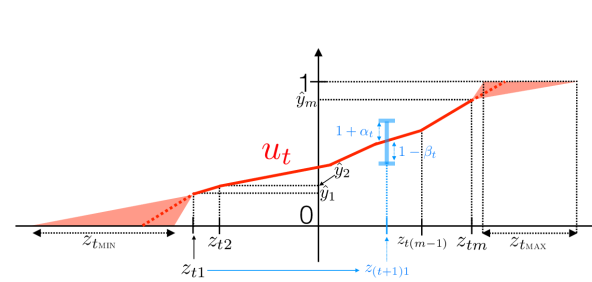
Figure 3: Inverse link $u$ of a proper canonical loss learned (red), as computable in fit ($z_{ti}\stackrel{{\scriptstyle\mathrm{.}}}{{=}}\bm{w}_{t}^{\top}\bm{x}_{i}$). In blue, we have depicted the stability constraint in the update of the link (Definition 3). Stability imposes just a constraint in the change of inverse link for a single example. It does not impose any constraint on the classifier update (which, in this example, is significant for example $(\bm{x}_{1},y_{1})$, see text).

$\triangleright$ Analysis of BregmanTron We are now ready to analyze the BregmanTron. Our main result shows that provided the link does not change too much between iterations, we are guaranteed to decrease the following loss:

$$\ell^{r}_{t}(S,\bm{w}_{t^{\prime}}) \stackrel{{\scriptstyle\mathrm{.}}}{{=}} \mathbb{E}_{{S}}[D_{U_{r}^{\star}}(y\|u_{t}(\bm{w}_{t^{\prime}}^{\top}\bm{x}))]\>\>,$$ (19)

for $r,t,t^{\prime}=1,2,...$, which gives (1) for $-\underline{L}\stackrel{{\scriptstyle\mathrm{.}}}{{=}}U_{r}^{\star}$, $u_{t}\stackrel{{\scriptstyle\mathrm{.}}}{{=}}\psi^{-1}$ and $h(\bm{x})\stackrel{{\scriptstyle\mathrm{.}}}{{=}}\bm{w}_{t^{\prime}}^{\top}\bm{x}$. We do not impose $r=t$, as our algorithm incorporates a step of proper composite fitting of the next link given the current loss.

We formalise the stability of the link below.

Definition 3

Let $\alpha_{t},\beta_{t}\geq 0$. BregmanTron is $(\alpha_{t},\beta_{t})$-stable at iteration $t$ iff the solution $\hat{\bm{y}}_{t+1}$ in Step 3 satisfies $\hat{y}_{1}\in u_{t}(\bm{w}_{t+1}^{\top}\bm{x}_{1})\cdot[1-\beta_{t},1+\alpha_{t}]$.

Since $\hat{y}_{1}\stackrel{{\scriptstyle\mathrm{.}}}{{=}}u_{t+1}(\bm{w}_{t+1}^{\top}\bm{x}_{1})$ from fit, it comes that stability requires a bounded local change in inverse link for a single example (but implies a bounded change for all via the Lipschitz constraints in Step 3; this is explained in the proof of the main Theorem of this Section). We define the following mean operators (Patrini et al., 2014): $\hat{\bm{\mu}}_{y}\stackrel{{\scriptstyle\mathrm{.}}}{{=}}\mathbb{E}_{{\mathcal{S}}}[y\cdot\bm{x}]$ (sample), $\hat{\bm{\mu}}_{t}\stackrel{{\scriptstyle\mathrm{.}}}{{=}}\mathbb{E}_{{\mathcal{S}}}[\hat{y}_{t}\cdot\bm{x}],\forall t\geq 1$ (estimated), where $\hat{y}_{t}$ is defined in the BregmanTron. We also let $p^{*}_{t}\stackrel{{\scriptstyle\mathrm{.}}}{{=}}\max\{\mathbb{E}_{{S}}[y],\mathbb{E}_{{S}}[u_{t}(\bm{w}_{t+1}^{\top}\bm{x})]\}\>\>\in[0,1]$ denote the $\max$ estimated $\hat{\Pr}(\mathsf{Y}=1)$ using both our model and the sample $S$. Assume $p_{t}^{*}>0$ as otherwise the problem is trivial. Finally, $X\stackrel{{\scriptstyle\mathrm{.}}}{{=}}\max_{i}\|\bm{x}_{i}\|_{2}$ (we consider the $L_{2}$ norm for simplicity; our result holds for any norm on $\mathcal{X}$).

Definition 4

BregmanTron is said to be in the $\delta_{t}$-regime at iteration $t$, for some $\delta_{t}>0$ iff:

$$\|\hat{\bm{\mu}}_{y}-\hat{\bm{\mu}}_{t}\|_{2} \geq 2\sqrt{p^{*}_{t}\delta_{t}}X,\forall t.$$ (20)

To simplify the statement of our Theorem, we let $f(z)\stackrel{{\scriptstyle\mathrm{.}}}{{=}}z/(1+z)$, which satisfies $f(\overline{\mathbb{R}}_{+})=[0,1]$.

Theorem 5

Suppose that BregmanTron is in the $\delta_{t}$-regime at iteration $t$, and the following holds:

• in Step 1, the learning rate

  $$\upeta_{t} = \frac{1-\gamma_{t}}{2N_{t}X^{2}}\cdot\left(1-\frac{f(\delta_{t})(1+f(\delta_{t}))p^{*}_{t}X}{\|\hat{\bm{\mu}}_{y}-\hat{\bm{\mu}}_{t}\|_{2}}\right),$$

  for some user-fixed $\gamma_{t}\in\left[0,\sqrt{f\circ f(\delta_{t})/2}\right]$;

• in Step 3, $N_{t},n_{t}$ satisfy $\nicefrac{{N_{t}}}{{n_{t}}},\nicefrac{{N_{t-1}}}{{n_{t}}}\leq 1+f(\delta_{t})$.

Then if the BregmanTron is $(f(\delta_{t}),f(\delta_{t}))$-stable, then:

$$\ell^{t+1}_{t+1}(S,\bm{w}_{t+1}) \leq \ell^{t}_{t}(S,\bm{w}_{t})-\frac{p^{*}_{t}f(\delta_{t})}{n_{t}}.$$ (21)

(proof in App, Section 10) Explicitly, it can be shown that the learning rate at iteration $t$ lies in the following interval:

$$\upeta \in \frac{1-\gamma_{t}}{2N_{t}X^{2}}\cdot\left(1-\frac{\sqrt{\delta_{t}p^{*}_{t}}(2+\delta_{t})}{2(1+\delta_{t})^{2}}\cdot\left[\sqrt{\delta_{t}p^{*}_{t}},1\right]\right),$$

Theorem 5 essentially says that as long as $\hat{\bm{\mu}}_{y}\neq\hat{\bm{\mu}}_{t}$, we can hope to get better results. This is no surprise: the gradient step in Step 1 of BregmanTron is proportional to $\hat{\bm{\mu}}_{y}-\hat{\bm{\mu}}_{t}$.

The conditions on Steps 1 and 3 are easily enforceable at any step of the algorithm, so the Theorem essentially says that whenever the link does not change too much between iterations, we are guaranteed a decrease in the loss and therefore a better fit of the class probabilities. Stability is the only assumption made: unlike Kakade et al. (2011), no assumptions are made about Bayes rule or the distribution $\mathcal{D}$, and no constraints are put on the classifier $\bm{w}$.

We can also choose to enforce stability in the update of $u$ in Step 3. Interestingly, while this restricts the choice of links (at least when $\|\hat{\bm{\mu}}_{y}-\hat{\bm{\mu}}_{t}\|_{2}$ is small), this guarantees the bound in (21) at no additional cost or assumption.

Corollary 6

Suppose BregmanTron is run with so that in Step 3, constraint $\hat{y}_{1}\geq 0$ is replaced by

$$\hat{y}_{1} \in u_{t}(\bm{w}_{t+1}^{\top}\bm{x}_{1})\cdot[1-\beta_{t},1+\alpha_{t}],$$ (22)

and all other constraints are kept the same. Suppose BregmanTron is in the $\delta_{t}$-regime at iteration $t$, parameters $\upeta_{t},N_{t},n_{t}$ are fixed as in Theorem 5 and furthermore $\alpha_{t},\beta_{t}\in[0,f(\delta_{t})]$. Then (21) holds.

(proof in App, Section 11) There exists an alternative reading of Corollary 6: there exists a way to fix the key parameters ($\upeta_{t},n_{t},N_{t},\alpha_{t},\beta_{t}$) at each iteration such that a decrease of the loss is guaranteed if our current estimate of the sample mean operator, $\hat{\bm{\mu}}_{t}$, is not good enough.

5 Discussion

Bregman divergences have had a rich history outside of convex optimisation, where they were introduced (Bregman, 1967). They are the canonical distortions on the manifold of parameters of exponential families in information geometry (Amari & Nagaoka, 2000), they have been introduced in normative economics in several contexts (Magdalou & Nock, 2011; Shorrocks, 1980). In machine learning, their re-discovery was grounded in their representation and algorithmic properties, starting with the work of M. Warmuth and collaborators (Helmbold et al., 1995; Herbster & Warmuth, 1998), later linked back to exponential families (Azoury & Warmuth, 2001), and then axiomatized in unsupervised learning (Banerjee et al., 2004, 2005), and then in supervised learning (See Section 4).

We do not investigate in this paper the generalization abilities of BregmanTron. It either follows from classical uniform convergence bounds applied to the convex surrogate of any proper canonical loss (which is always 1-Lipschitz), for which refer to Bartlett & Mendelson (2002, Section 2) and references therein for available tools, or it would justify a paper of its own if we want to directly investigate the approximation of Bayes rule, a problem that also entails the prospective problems presented below.

The setting of the BregmanTron raises two questions, the first of which is crucial for the algorithm. We make no assumption about the optimal link, which resorts to a powerful agnostic view of machine learning chased in a number of works (Bousquet et al., 2019), but it makes much more sense if we can prove that the link fit by fit belongs to a set with reasonable approximations of the target. This set contains piecewise affine links, which is a bit more general than Definition 2 but matches the links learned by the BregmanTron. We remove the index notation $T$ in $u_{T}$ and $z_{T.}$, and consider the following $\ell_{1}$ restricted discrepancy,

$$E(u,\ell) \stackrel{{\scriptstyle\mathrm{.}}}{{=}} \int_{z_{1}}^{z_{m}}|(-\underline{L}^{\prime})^{-1}(z)-u(z)|\mathrm{d}z,$$ (23)

where $\ell$ is proper canonical with invertible canonical link. It is restricted because we do not consider set $(-\infty,z_{1})\cup(z_{m},+\infty)$, whose fitting in fact does not depend on data (see Figure 3). Denote $\mathcal{U}_{n,N}(\bm{w},S)$ the set of piecewise affine links with non-$\{0,1\}$ breakout points on abscissae $z_{1},z_{2},...,z_{m}$ ($\bm{w}^{\top}\bm{x}_{i}\stackrel{{\scriptstyle\mathrm{.}}}{{=}}z_{i}<z_{i+1}\stackrel{{\scriptstyle\mathrm{.}}}{{=}}\bm{w}^{\top}\bm{x}_{i+1},\forall i\in\{0,1,...,m-1\}$, wlog), satisfying Definition 2. Let $\|.\|$ be any norm on $\mathcal{X}$ and $\|.\|_{*}$ its dual. For any $\varepsilon>0$, $G_{\varepsilon}(S)$ is the graph whose vertices are the observations in $S$ and an edge links $\bm{x},\bm{x}^{\prime}\in S$ iff $\|\bm{x}-\bm{x}^{\prime}\|\leq\varepsilon$. $G$ is said 2-vertex-connected iff it is connected when any single vertex is removed, which is a lightweight condition that essentially prevents the graph from being constituted of two almost separate subgraphs.

Lemma 7

For any $S$ of size $m$, any $\varepsilon>0$ such that $G_{\varepsilon}(S)$ is 2-vertex-connected and any proper canonical loss $\ell$, $\exists n,N\ll\infty$ such that $\inf_{u\in\mathcal{U}_{n,N}(\bm{w},S)}E(u,\ell)\leq 2Nm\varepsilon^{2}\cdot\|\bm{w}\|_{*}^{2}$.

Crucially, $N$ can be much smaller than the Lipschitz constant of $(-\underline{L}^{\prime})^{-1}$. Lemma 7 does guarantee that the set of links in which the BregmanTron finds $u_{T}$ is powerful enough to approximate a link provided we sample enough examples to drag $\varepsilon$ small enough while guaranteeing $G_{\varepsilon}(S)$ 2-connected. This does not require i.i.d. sampling but would require additional assumptions about $\mathcal{X}$ to be tractable (such as boundedness), or the possibility of active learning in $\mathcal{X}$. This also does not guarantee that fit finds a link with small $E(.,\ell)$, and this brings us to our second question: is it possible that (near-)optimal solutions contain very "different" couples $(u,\bm{w})$, for which useful notion(s) of "different" ? This, we believe, has ties with the transferability of the loss.

6 Experimental results

We present experiments illustrating:

1. the viability of the BregmanTron as an alternative to classic GLM or SlIsotron learning.

2. the nature of the loss functions learned by the BregmanTron, which are potentially asymmetric.

3. the potential of using the loss function learned by the BregmanTron as input to some downstream learner.

$\triangleright$ Predictive performance of BregmanTron We compare BregmanTron as a generic binary classification method against the following baselines: logistic regression, GLMTron (Kakade et al., 2011) with $u(\cdot)$ the sigmoid, and SlIsotron. We also consider two variants of BregmanTron: one where in Step 4 we do not find the global optimum (${\textsc{Bregman{}T{}ron}}_{\mathrm{approx}}$), but rather a feasible solution with minimal $\hat{y}_{m}$; and another where in Step 4 we fit against the labels, rather than $\hat{y}_{t}$ (${\textsc{Bregman{}T{}ron}}_{\mathrm{label}}$).

In all experiments, we fix the following parameters for BregmanTron: we use a constant learning rate of $\eta=1$ to perform the gradient update in Step 1, For Step 3, we fix $n_{t}=10^{-2}$ and $N_{t}=1$ for all iterations.

We compare performance on two standard benchmark datasets, the MNIST digits (mnist) and the fashion MNIST (fmnist). We converted the former to a binary classification problem of the digits 0 versus 8, and the latter of the odd versus even classes. We also consider a synthetic dataset (synth), comprising 2D Gaussian class-conditionals with means $\pm(1,1)$ and identity covariance matrix. The Bayes-optimal solution for $\Pr(\mathsf{Y}=1\mid\mathsf{X})$ can be derived in this case: it takes the form of a sigmoid, as assumed by logistic regression, composed with a linear model proportional to the expectation. In this case therefore, logistic regression works on a search space much smaller than BregmanTron and guaranteed to contain the optimum.

On a given dataset, we measure the predictive performance for each method via the area under the ROC curve. This assesses the ranking quality of predictions, which provides a commensurate means of comparison; in particular the BregmanTron optimises for a bespoke loss function that can be vastly different from the square-loss.

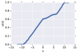
(a) synth.

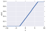
(b) mnist

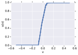
(c) fmnist

Figure 4: Link functions estimated by BregmanTron on each dataset. On all datasets, the losses are seen to be (slightly) asymmetric around $\frac{1}{2}$, i.e., $u(v)\neq 1-u(-v)$. In particular, $u(0)\neq\frac{1}{2}$.

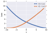
(a) synth.

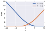
(b) mnist

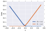
(c) fmnist

Figure 5: Loss functions estimated by BregmanTron on each dataset. The losses are (slightly) asymmetric, and have the flavour of the square-hinge loss; this is a consequence of the linear interpolation used when fitting.

Table 1 summarises the results. We make three observations. First, BregmanTron is consistently competitive with the mature baseline of logistic regression. Interestingly, this is even so on the synth problem, wherein logistic regression is correctly specified. Although the difference in performance here is minor, it does illustrate that BregmanTron can infer a meaningful pair of $(u,\bm{w})$.

Second, BregmanTron and BregmanTron_label are generally superior to the performance of the SlIsotron. We attribute this to the latter’s reliance on an isotonic regression step to fit the links, as opposed to a Bregman regularisation.

Third, while BregmanTron_approx also performs reasonably, it is typically worse than the full BregmanTron. This illustrates the value of (at least approximately) solving Step 4 in the BregmanTron. Further, while BregmanTron_label generally performs slightly worse than standard BregmanTron, it remains competitive. A formal analysis of this method would be of interest in future work.

	synth	mnist	fmnist
Logistic regression	92.2%	99.9%	98.5%
GLMTron	92.2%	99.6%	98.1%
SlIsotron	91.6%	94.6%	90.7%
BregmanTronapprox	92.2%	99.3%	94.6%
BregmanTronlabel	90.1%	99.6%	97.7%
BregmanTron	92.3%	99.7%	97.9%

Table 1: Test set AUC of various methods on binary classification datasets. See text for details.

$\triangleright$ Illustration of learned losses As with the SlIsotron, a salient feature of BregmanTron is the ability to automatically learn a link function. Unlike the SlIsotron, however, the link in the BregmanTron has an interpretation of corresponding to a canonical loss function.

Figure 4 illustrates the link functions learned by BregmanTron on each dataset. We see that these links are generally asymmetric about $\frac{1}{2}$. This is in contrast to standard link functions such as the sigmoid. Recall that each link corresponds to an underlying canonical loss, given by $\ell^{\prime}(y,v)=u(v)-y$. Asymmetry of $u(\cdot)$ thus manifests in $\ell(+1,v)\neq\ell(-1,-v)$. We illustrate these implicit canonical losses in Figure 5. As a consequence of the links not being symmetric around $\frac{1}{2}$, the losses on the positive and negative classes are not symmetric for the synth dataset. This is unlike the theoretical link, but the theoretical link may not be optimal at all on sampled data. This, we believe, also illustrates the intriguing potential of the BregmanTron to detect and exploit hidden asymmetries in the underlying data distribution.

$\triangleright$ Transferability of the loss between domains Finally, we illustrate the potential of “recycling” the loss function implicitly learned by BregmanTron for some other task. We take the fmnist dataset, and first train BregmanTron to classify the classes 0 versus 6 (“T-shirt” versus “Shirt”). This classifier achieves an AUC of $0.85$, which is competitive with the logistic regression AUC of $0.86$.

Recall that BregmanTron gives us a learned link $u$, which per the above discussion also defines an implicit canonical loss. By training a classifier to distinguish classes 2 versus 4 (“Pullover” versus “Coat”) using this loss function, we achieve an AUC of $\mathbf{0.879}$. This slightly outperforms the $\mathbf{0.877}$ AUC of logistic regression, and is also competitive with the $\mathbf{0.879}$ AUC attained by training BregmanTron directly on classes 2 versus 4. This indicates that the loss learned by BregmanTron on one domain could be useful in related domains to another classification algorithms just training a classifier. To properly develop this possibility is out of the scope of this paper, and as far as we know such a perspective is new in machine learning.

7 Conclusion

Fitting a loss that complies with Bayes decision theory implies not just to be able to learn a classifier, but also a canonical link of a proper loss, and therefore a proper canonical loss. In a 2011 seminal work, Kakade et al. made with the SLIsotron algorithm the first attempt at solving this bigger picture of supervised learning. We propose in this paper a more general approach grounded on a general Bregman formulation of differentiable proper canonical losses.

Experiments tend to confirm the ability of our approach, the BregmanTron, to beat the SLIsotron, and compete with classical supervised approaches even when they are informed with the optimal choice of link. Interestingly, they seem to illustrate the importance of a stability requirement made by our theory. More interesting is perhaps the observation that the loss learned by the BregmanTron on one domain can be useful to other learning algorithms to fit classifiers on related domains, a transferability property of the loss learned that deserves further thought.

Appendix

8 Factsheet on Bregman divergences

We summarize in this section the results we use (both in the main file and in this App) related to Bregman divergence with convex generator $F$,

$$D_{F}(z\|z^{\prime}) \stackrel{{\scriptstyle\mathrm{.}}}{{=}} F(z)-F(z^{\prime})-(z-z^{\prime})F^{\prime}(z^{\prime}),$$ (24)

where we assume for the sake of simplicity that $F$ is twice differentiable.

$\triangleright$ General properties – $D_{F}$ is always non-negative, convex in its left parameter, but not always in its right parameter. Only the divergences corresponding to $F(z)\propto z^{2}$ are symmetric (Boissonnat et al., 2010).

$\triangleright$ $D_{F}$ is locally proportional to the square loss – assuming second order differentiability, we have (Nock et al., 2008):

$$\forall z,z^{\prime},\exists c\in[z\wedge z^{\prime},z\vee z^{\prime}]:D_{F}(z\|z^{\prime}) = \frac{F^{\prime\prime}(c)}{2}\cdot(z-z^{\prime})^{2}.$$ (25)

$\triangleright$ Bregman triangle equality – also called the three points property (Nock et al., 2008, 2016),

$$\forall z,z^{\prime},z^{\prime\prime},D_{F}(z\|z^{\prime\prime}) = D_{F}(z\|z^{\prime})+D_{F}(z^{\prime}\|z^{\prime\prime})+(F^{\prime}(z^{\prime\prime})-F^{\prime}(z^{\prime}))(z^{\prime}-z).$$ (26)

$\triangleright$ Invariance to affine terms – for any affine function $G(z)$ (Boissonnat et al., 2010),

$$\forall z,z^{\prime},D_{F+G}(z\|z^{\prime}) = D_{F}(z\|z^{\prime}).$$ (27)

$\triangleright$ Dual symmetry – letting $F^{\star}$ denote the convex conjugate of $F$, we have (Nock et al., 2016),

$$\forall z,z^{\prime},D_{F}(z\|z^{\prime}) = D_{F^{\star}}(F^{\prime}(z^{\prime})\|F^{\prime}(z)).$$ (28)

$\triangleright$ The right population minimizer is the mean – we have (Banerjee et al., 2004),

$$\arg\min_{z}\mathbb{E}_{\mathsf{Z}}[D_{F}(\mathsf{Z}\|z)] = \mathbb{E}_{\mathsf{Z}}[\mathsf{Z}]\stackrel{{\scriptstyle\mathrm{.}}}{{=}}\mu(\mathsf{Z}).$$ (29)

$\triangleright$ Bregman information – the Bregman information of random variable $\mathsf{Z}$, defined as $I_{F}(\mathsf{Z})\stackrel{{\scriptstyle\mathrm{.}}}{{=}}\min_{z}\mathbb{E}_{\mathsf{Z}}[D_{F}(\mathsf{Z}\|z)]$, satisfies (Banerjee et al., 2004)

$$I_{F}(\mathsf{Z}) = \mathbb{E}_{\mathsf{Z}}[D_{F}(\mathsf{Z}\|\mu(\mathsf{Z}))].$$ (30)

9 Proof of Theorem 1

($\Rightarrow$) The proof assumes basic knowledge about proper losses as in Reid & Williamson (2010) (and references therein) for example. It comes from Reid & Williamson (2010, Theorem 1, Corollary 3) and Shuford et al. (1966) that a differentiable function defines a proper loss iff there exists a Riemann integrable (eventually improper in the integrability sense) function $w:(0,1)\rightarrow\mathbb{R}_{+}$ such that:

$$w(c)=\frac{\ell^{\prime}_{-1}(c)}{c}=-\frac{\ell^{\prime}_{1}(c)}{1-c}\>\>,\forall c\in(0,1).$$ (31)

To simplify notations, we slightly abuse notations and let $\underline{L}^{\prime\prime}\stackrel{{\scriptstyle\mathrm{.}}}{{=}}-w$ and define $\underline{L}^{\prime}(u)\stackrel{{\scriptstyle\mathrm{.}}}{{=}}\int_{a}^{u}\underline{L}^{\prime\prime}(z)\mathrm{d}z$ for some adequately chosen constant $a$ (for example, $a=1/2$ for symmetric proper canonical losses Nock & Nielsen (2009, 2008)). We denote such a representation of loss functions their integral representation (Reid & Williamson, 2010, eq. (5)), as it gives:

$$\ell_{1}(c) = \int_{c}^{1}-(1-u)\underline{L}^{\prime\prime}(u)\mathrm{d}u,$$ (32)

from which we derive by integrating by parts,

$$\ell_{1}(c) = -\left[(1-u)\underline{L}^{\prime}(u)\right]_{c}^{1}-\int_{c}^{1}\underline{L}^{\prime}(u)\mathrm{d}u$$ (33)

$$= (1-c)\underline{L}^{\prime}(c)-\underline{L}(1)+\underline{L}(c)$$

$$= (-\underline{L})(1)-(-\underline{L})(c)-(1-c)(-\underline{L})^{\prime}(c)$$ (34)

$$= D_{-\underline{L}}(1\|c),$$ (35)

Where $D_{-\underline{L}}$ is the Bregman divergence with generator $-\underline{L}$ (we remind that the conditional Bayes risk of a proper loss is concave (Reid & Williamson, 2010, Section 3.2)). We get similarly for the partial loss $\ell_{-1}$ (Reid & Williamson, 2010, eq. (5)):

$$\ell_{-1}(c) = -\int_{0}^{c}u\underline{L}^{\prime\prime}(u)\mathrm{d}u$$ (36)

$$= -\left[u\underline{L}^{\prime}(u)\right]_{0}^{c}+\int_{0}^{c}\underline{L}^{\prime}(u)\mathrm{d}u$$

$$= -c\underline{L}^{\prime}(c)+\underline{L}(c)-\underline{L}(0)$$

$$= (-\underline{L})(0)-(-\underline{L})(c)-(0-c)(-\underline{L})^{\prime}(c)$$ (37)

$$= D_{-\underline{L}}(0\|c).$$ (38)

We now replace $c$ by the inverse of the link chosen, $\psi$, and we get for any proper composite loss:

$$\ell(y^{*},z) \stackrel{{\scriptstyle\mathrm{.}}}{{=}} \llbracket y^{*}=1\rrbracket\cdot\ell_{1}({\psi}^{-1}(z))+\llbracket y^{*}=-1\rrbracket\cdot\ell_{-1}({\psi}^{-1}(z))$$ (39)

$$= D_{-\underline{L}}(y\|{\psi}^{-1}(z)),$$

as claimed for the implication $\Rightarrow$. The identity

$$D_{-\underline{L}}(y\|{\psi}^{-1}(z)) = D_{(-\underline{L})^{\star}}({-\underline{L}^{\prime}}\circ{\psi}^{-1}(z)\|{-\underline{L}^{\prime}}(y))$$ (40)

follows from the dual symmetry property of Bregman divergences (Boissonnat et al., 2010; Nock et al., 2016).

($\Leftarrow$) Let $\ell(y^{*},z)\stackrel{{\scriptstyle\mathrm{.}}}{{=}}D_{-F}(y\|g^{-1}(z))$, some Bregman divergence, where $g:[0,1]\rightarrow\mathbb{R}$ is invertible. Let $\ell_{p}(y^{*},c):\mathcal{Y}\times[0,1]\rightarrow\overline{\mathbb{R}}$ defined by $\ell_{p}(y^{*},c)\stackrel{{\scriptstyle\mathrm{.}}}{{=}}\ell(y^{*},g(c))$. We know that the right population minimizer of any Bregman divergence is the expectation (Banerjee et al., 2004; Nock et al., 2016), so $\pi\in\arg\inf_{u}\mathsf{E}_{\mathsf{Y}\sim\pi}\ell_{p}(\mathsf{Y},u),\forall\pi\in[0,1]$ and $\ell_{p}$ is proper. Therefore $\ell$ is proper composite since $g$ is invertible. The conditional Bayes risk of $\ell_{p}$ is therefore by definition:

$$\underline{L}(\pi) \stackrel{{\scriptstyle\mathrm{.}}}{{=}} \mathsf{E}_{\mathsf{Y}\sim\pi}\ell_{p}(\mathsf{Y},\pi)$$ (41)

$$= F(\pi)+G(\pi)$$ (42)

where $G(\pi)\stackrel{{\scriptstyle\mathrm{.}}}{{=}}-\pi F(1)-(1-\pi)F(0)$ is affine. Since a Bregman divergence is invariant by addition of an affine term to its generator (27), we get

$$\ell_{p}(y^{*},c) = D_{-F}(y\|c)$$ (43)

$$= D_{-\underline{L}}(y\|c).$$ (44)

We now check that if $g=-F^{\prime}$ then $\ell$ is proper canonical. It comes from (42) $(-F^{\prime})^{-1}(z)=({-\underline{L}^{\prime}})^{-1}(z+K)$ where $K\stackrel{{\scriptstyle\mathrm{.}}}{{=}}-(F(1)-F(0))$ is a constant, which is still the inverse of the canonical link since it is defined up to multiplication or addition by a scalar (Buja et al., 2005). Hence, if $g=-F^{\prime}$ then $\ell(y^{*},z)$ is proper canonical. Otherwise as previously argued it is proper composite with link $g$ in the more general case. This completes the proof for the implication $\Leftarrow$, and ends the proof of Theorem 1.

Remark: symmetric proper canonical losses (such as the logistic, square or Matsushita losses) admit $\underline{L}(0)=\underline{L}(1)$ Nock & Nielsen (2009, 2008). Hence (42) enforces $\forall\pi\in[0,1]$

$$\pi(F(0)-F(1))=\underline{L}(0)=\underline{L}(1)=(1-\pi)(F(1)-F(0)),$$ (45)

resulting in $F(1)=F(0)$ and therefore enforcing the constraint $K=0$ above.

10 Proof of Theorem 5

10.1 Helper results about BregmanTron and fit

To prove the Theorem, we first show several simple helper results. The first is a simple consequence of the design of $u_{t}$. We prove it for the sake of completeness.

Lemma 8

Let $u_{t}$ be the function output by fit in BregmanTron. Let $z_{m}\stackrel{{\scriptstyle\mathrm{.}}}{{=}}u_{t}^{-1}(0)$ and $z_{m}\stackrel{{\scriptstyle\mathrm{.}}}{{=}}u_{t}^{-1}(1)$. Let $U_{t}$ be defined as in (16) (main body, with $u\leftarrow u_{t}$). The following holds true on $u_{t}$

$$n_{t-1}\cdot(z-z^{\prime})\leq u_{t}(z)-u_{t}(z^{\prime})\leq N_{t-1}\cdot(z-z^{\prime})\>\>,$$ (46)

$$\frac{1}{N_{t-1}}\cdot(p-p^{\prime})\leq u^{-1}_{t}(p)-u^{-1}_{t}(p^{\prime})\leq\frac{1}{n_{t-1}}\cdot(p-p^{\prime})\>\>,$$ (47)

$\forall z_{m}\leq z^{\prime}\leq z\leq z_{M}$, $\forall 0\leq p^{\prime}\leq p\leq 1$, and the following holds true on $U_{t}$:

$$\frac{(p-p^{\prime})^{2}}{2N_{t-1}}\leq D_{U^{\star}_{t}}(p\|p^{\prime})\leq\frac{(p-p^{\prime})^{2}}{2n_{t-1}}.$$ (48)

Proof.

We show the right-hand side of ineq. (46). The left hand side of (46) follows by symmetry and ineq (47) follow after a variable change from ineq (46). The proof is a rewriting of the mean-value Theorem for subdifferentials: consider for example the case $u_{t}(b)-u_{t}(a)=N^{\prime}(b-a)$ with $N^{\prime}>N_{t-1}$ for some $z_{m}<a<b<z_{M}$. Let

$$v(z) \stackrel{{\scriptstyle\mathrm{.}}}{{=}} u_{t}(z)-u_{t}(b)+N^{\prime}(b-z)\>\>,$$ (49)

and since $v(a)=v(b)=0$, let $z_{*}\stackrel{{\scriptstyle\mathrm{.}}}{{=}}\arg\min_{z}v(z)$, assuming wlog that the min exists. Then $v(z)\geq v(z_{*})$, and equivalently $u_{t}(z)-u_{t}(b)+N^{\prime}(b-z)\geq u_{t}(z_{*})-u_{t}(b)+N^{\prime}(b-z_{*})$ ($\forall z\in[a,b]$), which, after reorganising, gives $u_{t}(z)\geq u_{t}(z_{*})+N^{\prime}(z-z_{*})$, implying $N^{\prime}\in\partial u_{t}(z_{*})$. Pick now $a\leq z^{\prime}_{*}<z_{*}<z^{\prime\prime}_{*}\leq b$ that are linked to $z_{*}$ by a line segment in $u_{t}$. At least one of the two segments has slope $\geq N^{\prime}$, which is impossible since $N^{\prime}>N_{t-1}$ and yields a contradiction. The case $a=z_{m}$ xor $b=z_{M}$ reduces to a single segment with slope $\geq N^{\prime}$, also impossible.

We now show (48). Let

$$V(p) \stackrel{{\scriptstyle\mathrm{.}}}{{=}} U^{\star}_{t}(b)-U^{\star}_{t}(p)-(b-p)u^{-1}_{t}(z)-A(b-p)^{2},$$ (50)

(remind that $(U^{\star}_{t})^{\prime}=u^{-1}_{t}$) where $A$ is chosen so that $V(a)=0$, which implies since $V(b)=0$ that $\exists c\in(a,b),0\in\partial V(c)$. We have $\partial V(c)\ni-(b-c)c^{\prime}-2A(c-b)$ for any $c^{\prime}\in\partial u^{-1}_{t}(c)$, implying $A=c^{\prime}/2$ for some $c^{\prime}\in\partial u^{-1}_{t}(c)$. Solving for $V(a)=0$ yields $D_{U^{\star}_{t}}(b\|a)=(c^{\prime}/2)(b-a)^{2}$ for some $c^{\prime}\in\partial u^{-1}_{t}$ and since $\mathrm{Im}\partial u^{-1}_{t}\subset[1/N_{t-1},1/n_{t-1}]$ from (47), we get

$$\frac{(b-a)^{2}}{2N_{t-1}}\leq D_{U^{\star}_{t}}(b\|a)\leq\frac{(b-a)^{2}}{2n_{t-1}},$$ (51)

as claimed. ∎

Note that we indeed have $\hat{y}_{1}\stackrel{{\scriptstyle\mathrm{.}}}{{=}}u_{t+1}(\bm{w}_{t+1}^{\top}\bm{x}_{1})$ by the design of Step 4 in BregmanTron. The second result we need is a direct consequence of Step 3 in BregmanTron.

Lemma 9

The following holds for any $t\geq 1,i\in[m]$,

$$u_{t+1}(\bm{w}_{t+1}^{\top}\bm{x}_{i}) \in u_{t}(\bm{w}_{t+1}^{\top}\bm{x}_{i})\cdot\left[\min\left\{1-\beta_{t},\frac{n_{t}}{N_{t}}\right\},\max\left\{1+\alpha_{t},\frac{N_{t}}{n_{t}}\right\}\right],$$ (52)

where $\alpha_{t},\beta_{t}\geq 0$ are the stability property parameters at the current iteration of BregmanTron, as defined in Definition 3 (main file).

Proof.

We prove the upperbound in (52) by induction. Assuming the property holds for $\bm{x}_{i}$ and considering $\bm{x}_{i+1}$ (recall that indexes are ordered in increasing value of $\bm{w}_{t+1}^{\top}\bm{x}_{i}$, see Step 2 in BregmanTron), we obtain

$$u_{t+1}(\bm{w}_{t+1}^{\top}\bm{x}_{{i+1}}) \leq u_{t+1}(\bm{w}_{t+1}^{\top}\bm{x}_{{i}})+N_{t}\bm{w}_{t+1}^{\top}(\bm{x}_{i+1}-\bm{x}_{i})$$ (53)

$$\leq u_{t+1}(\bm{w}_{t+1}^{\top}\bm{x}_{{i}})+\frac{N_{t}}{n_{t}}\cdot\left(u_{t}(\bm{w}_{t+1}^{\top}\bm{x}_{{i+1}})-u_{t}(\bm{w}_{t+1}^{\top}\bm{x}_{{i}})\right)$$ (55)

$$=\frac{N_{t}}{n_{t}}u_{t}(\bm{w}_{t+1}^{\top}\bm{x}_{{i+1}})+u_{t+1}(\bm{w}_{t+1}^{\top}\bm{x}_{{i}})-\frac{N_{t}}{n_{t}}\cdot u_{t}(\bm{w}_{t+1}^{\top}\bm{x}_{{i}})\>\>.$$

The first inequality comes from the right interval constraint in problem (12) applied to $u_{t+1}$, ineq. (55) comes from Lemma 8 applied to $u_{t}$. We now have two cases.

Case 1 If $N_{t}/n_{t}>1+\alpha_{t}$, using the induction hypothesis (52) yields $u_{t+1}(\bm{w}_{t+1}^{\top}\bm{x}_{{i}})\leq(N_{t}/n_{t})\cdot u_{t}(\bm{w}_{t+1}^{\top}\bm{x}_{i})$ and so (55) becomes

$$u_{t+1}(\bm{w}_{t+1}^{\top}\bm{x}_{{i+1}}) \leq \frac{N_{t}}{n_{t}}u_{t}(\bm{w}_{t+1}^{\top}\bm{x}_{{i+1}})+\frac{N_{t}}{n_{t}}u_{t}(\bm{w}_{t+1}^{\top}\bm{x}_{{i}})-\frac{N_{t}}{n_{t}}u_{t}(\bm{w}_{t+1}^{\top}\bm{x}_{{i}})$$ (56)

$$=\frac{N_{t}}{n_{t}}u_{t}(\bm{w}_{t+1}^{\top}\bm{x}_{{i+1}}).$$

Case 2 If $N_{t}/n_{t}\leq 1+\alpha_{t}$, we have this time from the induction hypothesis $u_{t+1}(\bm{w}_{t+1}^{\top}\bm{x}_{{i}})\leq(1+\alpha_{t})\cdot u_{t}(\bm{w}_{t+1}^{\top}\bm{x}_{i})$, and so we get from (55),

$$u_{t+1}(\bm{w}_{t+1}^{\top}\bm{x}_{{i+1}}) \leq \frac{N_{t}}{n_{t}}u_{t}(\bm{w}_{t+1}^{\top}\bm{x}_{{i+1}})+\left(1+\alpha_{t}-\frac{N_{t}}{n_{t}}\right)\cdot u_{t}(\bm{w}_{t+1}^{\top}\bm{x}_{{i}})$$ (58)

$$\leq \frac{N_{t}}{n_{t}}u_{t}(\bm{w}_{t+1}^{\top}\bm{x}_{{i+1}})+\left(1+\alpha_{t}-\frac{N_{t}}{n_{t}}\right)\cdot u_{t}(\bm{w}_{t+1}^{\top}\bm{x}_{{i+1}})$$

$$=(1+\alpha_{t})u_{t}(\bm{w}_{t+1}^{\top}\bm{x}_{{i+1}})\>\>,$$

where (58) holds because $\bm{w}_{t+1}^{\top}\bm{x}_{{i}}\leq\bm{w}_{t+1}^{\top}\bm{x}_{{i+1}}$ (by assumption) and $u_{t}$ is non-decreasing.

The proof of the lowerbound in (52) follows from the following "symmetric" induction, noting first that the second constraint in problem (12) (main file) implies the base case, $u_{t+1}(\bm{w}_{t+1}^{\top}\bm{x}_{1})\geq(1-\beta_{t})u_{t}(\bm{w}_{t+1}^{\top}\bm{x}_{1})$, and then, for the general index $i>1$,

$$u_{t+1}(\bm{w}_{t+1}^{\top}\bm{x}_{{i+1}}) \geq u_{t+1}(\bm{w}_{t+1}^{\top}\bm{x}_{{i}})+n_{t}\bm{w}_{t+1}^{\top}(\bm{x}_{i+1}-\bm{x}_{i})$$ (59)

$$\geq u_{t+1}(\bm{w}_{t+1}^{\top}\bm{x}_{{i}})+\frac{n_{t}}{N_{t}}\cdot\left(u_{t}(\bm{w}_{t+1}^{\top}\bm{x}_{{i+1}})-u_{t}(\bm{w}_{t+1}^{\top}\bm{x}_{{i}})\right)$$ (61)

$$=\frac{n_{t}}{N_{t}}\cdot u_{t}(\bm{w}_{t+1}^{\top}\bm{x}_{{i+1}})+u_{t+1}(\bm{w}_{t+1}^{\top}\bm{x}_{{i}})-\frac{n_{t}}{N_{t}}\cdot u_{t}(\bm{w}_{t+1}^{\top}\bm{x}_{{i}}).$$

The first inequality comes from the left interval constraint in problem (12) applied to $u_{t+1}$, ineq. (61) comes from Lemma 8 applied to $u_{t}$. Similarly to the upperbound in (52), we now have two cases.

Case 1 If $n_{t}/N_{t}\leq 1-\beta_{t}$, using the induction hypothesis (52) yields $u_{t+1}(\bm{w}_{t+1}^{\top}\bm{x}_{{i}})\geq(n_{t}/N_{t})\cdot u_{t}(\bm{w}_{t+1}^{\top}\bm{x}_{i})$ and so (61) becomes

$$u_{t+1}(\bm{w}_{t+1}^{\top}\bm{x}_{{i+1}}) \geq \frac{n_{t}}{N_{t}}\cdot u_{t}(\bm{w}_{t+1}^{\top}\bm{x}_{{i+1}})+\frac{n_{t}}{N_{t}}\cdot u_{t}(\bm{w}_{t+1}^{\top}\bm{x}_{i})-\frac{n_{t}}{N_{t}}\cdot u_{t}(\bm{w}_{t+1}^{\top}\bm{x}_{{i}})$$ (62)

$$=\frac{n_{t}}{N_{t}}\cdot u_{t}(\bm{w}_{t+1}^{\top}\bm{x}_{{i+1}}).$$

Case 2 If $n_{t}/N_{t}>1-\beta_{t}$, using the induction hypothesis (52) yields $u_{t+1}(\bm{w}_{t+1}^{\top}\bm{x}_{{i}})\geq(1-\beta_{t})\cdot u_{t}(\bm{w}_{t+1}^{\top}\bm{x}_{i})$ and so (61) becomes

$$u_{t+1}(\bm{w}_{t+1}^{\top}\bm{x}_{{i+1}}) \geq \frac{n_{t}}{N_{t}}\cdot u_{t}(\bm{w}_{t+1}^{\top}\bm{x}_{{i+1}})+(1-\beta_{t})\cdot u_{t}(\bm{w}_{t+1}^{\top}\bm{x}_{i})-\frac{n_{t}}{N_{t}}\cdot u_{t}(\bm{w}_{t+1}^{\top}\bm{x}_{{i}})$$ (64)

$$\geq \frac{n_{t}}{N_{t}}\cdot u_{t}(\bm{w}_{t+1}^{\top}\bm{x}_{{i}})+(1-\beta_{t})\cdot u_{t}(\bm{w}_{t+1}^{\top}\bm{x}_{i})-\frac{n_{t}}{N_{t}}\cdot u_{t}(\bm{w}_{t+1}^{\top}\bm{x}_{{i}})$$

$$=(1-\beta_{t})\cdot u_{t}(\bm{w}_{t+1}^{\top}\bm{x}_{i}).$$

(64) holds because $\bm{w}_{t+1}^{\top}\bm{x}_{{i}}\leq\bm{w}_{t+1}^{\top}\bm{x}_{{i+1}}$ (by assumption) and $u_{t}$ is non-decreasing. This achieves the proof of Lemma 9. ∎

We now analyze the following Bregman loss for $r,t,t^{\prime}=1,2,...$:

$$\ell^{r}_{t}(S,\bm{w}_{t^{\prime}}) \stackrel{{\scriptstyle\mathrm{.}}}{{=}} \mathbb{E}_{{S}}[D_{U_{r}^{\star}}(y\|u_{t}(\bm{w}_{t^{\prime}}^{\top}\bm{x}))]=\mathbb{E}_{{S}}\left[D_{U_{r}}(u_{r}^{-1}\circ u_{t}(\bm{w}_{t^{\prime}}^{\top}\bm{x})\|u_{r}^{-1}(y))\right]\>\>,$$ (65)

The key to the proof of Theorem 5 is the following Theorem which breaks down the bound that we have to analyze into several parts.

Theorem 10

For any $t\geq 1$,

$$\ell^{t+1}_{t+1}(S,\bm{w}_{t+1}) \leq \ell^{t}_{t}(S,\bm{w}_{t})-\mathbb{E}_{{S}}[D_{U_{t}}(\bm{w}_{t}^{\top}\bm{x}\|u^{-1}_{t}\circ u_{t+1}(\bm{w}_{t+1}^{\top}\bm{x}))]-L_{t+1}-Q_{t+1},$$

where

$$L_{t+1} \stackrel{{\scriptstyle\mathrm{.}}}{{=}} \mathbb{E}_{{S}}[(\bm{w}_{t}^{\top}\bm{x}-u^{-1}_{t}\circ u_{t+1}(\bm{w}_{t+1}^{\top}\bm{x}))\cdot(u_{t+1}(\bm{w}_{t+1}^{\top}\bm{x})-u_{t}(\bm{w}_{t+1}^{\top}\bm{x}))],$$

$$Q_{t+1} \stackrel{{\scriptstyle\mathrm{.}}}{{=}} \mathbb{E}_{{S}}[(\bm{w}_{t}^{\top}\bm{x}-u^{-1}_{t}\circ u_{t+1}(\bm{w}_{t+1}^{\top}\bm{x}))\cdot(u_{t}(\bm{w}_{t+1}^{\top}\bm{x})-y)]-\left(\frac{N_{t-1}}{n_{t}}-1\right)\cdot\ell^{t}_{t+1}(S,\bm{w}_{t+1}).$$

Proof.

We have the following derivations:

$$\ell^{t}_{t}(S,\bm{w}_{t}) = \mathbb{E}_{{S}}[D_{U_{t}^{\star}}(y\|u_{t}(\bm{w}_{t}^{\top}\bm{x}))]$$ (67)

$$= \mathbb{E}_{{S}}[D_{U_{t}^{\star}}(y\|u_{t+1}(\bm{w}_{t+1}^{\top}\bm{x}))]+\mathbb{E}_{{S}}[D_{U_{t}^{\star}}(u_{t+1}(\bm{w}_{t+1}^{\top}\bm{x})\|u_{t}(\bm{w}_{t}^{\top}\bm{x}))]$$

$$+\mathbb{E}_{{S}}[((U_{t}^{\star})^{\prime}(u_{t}(\bm{w}_{t}^{\top}\bm{x}))-(U_{t}^{\star})^{\prime}(u_{t+1}(\bm{w}_{t+1}^{\top}\bm{x})))\cdot(u_{t+1}(\bm{w}_{t+1}^{\top}\bm{x})-y)]$$

$$= \ell^{t}_{t+1}(S,\bm{w}_{t+1})+\mathbb{E}_{{S}}[D_{U_{t}}(\bm{w}_{t}^{\top}\bm{x}\|u^{-1}_{t}\circ u_{t+1}(\bm{w}_{t+1}^{\top}\bm{x}))]$$

$$+\underbrace{\mathbb{E}_{{S}}[(\bm{w}_{t}^{\top}\bm{x}-u^{-1}_{t}\circ u_{t+1}(\bm{w}_{t+1}^{\top}\bm{x}))\cdot(u_{t+1}(\bm{w}_{t+1}^{\top}\bm{x})-y)]}_{\stackrel{{\scriptstyle\mathrm{.}}}{{=}}\Delta_{t+1}}.$$

(67) follows from the Bregman triangle equality (26). (67) follows from $(U_{t}^{\star})^{\prime}\stackrel{{\scriptstyle\mathrm{.}}}{{=}}u_{t}^{-1}$ and (28). Reordering, we get:

$$\ell^{t}_{t+1}(S,\bm{w}_{t+1}) = \ell^{t}_{t}(S,\bm{w}_{t})-\mathbb{E}_{{S}}[D_{U_{t}}(\bm{w}_{t}^{\top}\bm{x}\|u^{-1}_{t}\circ u_{t+1}(\bm{w}_{t+1}^{\top}\bm{x}))]-\Delta_{t+1},$$ (68)

and we further split $\Delta_{t+1}$ in two: $\Delta_{t+1}\stackrel{{\scriptstyle\mathrm{.}}}{{=}}F_{t+1}+L_{t+1}$, where

$$F_{t+1} \stackrel{{\scriptstyle\mathrm{.}}}{{=}} \mathbb{E}_{{S}}[(\bm{w}_{t}^{\top}\bm{x}-u^{-1}_{t}\circ u_{t+1}(\bm{w}_{t+1}^{\top}\bm{x}))\cdot(u_{t}(\bm{w}_{t+1}^{\top}\bm{x})-y)],$$ (69)

$$L_{t+1} \stackrel{{\scriptstyle\mathrm{.}}}{{=}} \mathbb{E}_{{S}}[(\bm{w}_{t}^{\top}\bm{x}-u^{-1}_{t}\circ u_{t+1}(\bm{w}_{t+1}^{\top}\bm{x}))\cdot(u_{t+1}(\bm{w}_{t+1}^{\top}\bm{x})-u_{t}(\bm{w}_{t+1}^{\top}\bm{x}))].$$ (70)

We now have the following Lemma.

Lemma 11

The following holds for any $t\geq 0$:

$$\ell^{t+1}_{t+1}(S,\bm{w}_{t+1}) \leq \frac{N_{t-1}}{n_{t}}\cdot\ell^{t}_{t+1}(S,\bm{w}_{t+1}).$$ (71)

Proof.

We use Lemma 8 and we get:

$$D_{U^{*}_{t+1}}(p\|p^{\prime}) \leq \frac{1}{2n_{t}}\cdot(p-p^{\prime})^{2}$$ (72)

$$\leq \frac{N_{t-1}}{n_{t}}\cdot D_{U^{*}_{t}}(p\|p^{\prime})\>\>,$$

from which we just compute the expectation in $\ell^{.}_{t+1}(S,\bm{w}_{t+1})$ and get the result as claimed. ∎

Putting altogether (68), (69), (70) and Lemma 11 yields, $\forall t\geq 1$,

$$\ell^{t+1}_{t+1}(S,\bm{w}_{t+1}) \leq \ell^{t}_{t+1}(S,\bm{w}_{t+1})+\left(\frac{N_{t-1}}{n_{t}}-1\right)\cdot\ell^{t}_{t+1}(S,\bm{w}_{t+1})$$ (73)

$$= \ell^{t}_{t}(S,\bm{w}_{t})-\mathbb{E}_{{S}}[D_{U_{t}}(\bm{w}_{t}^{\top}\bm{x}\|u^{-1}_{t}\circ u_{t+1}(\bm{w}_{t+1}^{\top}\bm{x}))]-L_{t+1}$$

$$-\left(F_{t+1}-\left(\frac{N_{t-1}}{n_{t}}-1\right)\cdot\ell^{t}_{t+1}(S,\bm{w}_{t+1})\right),$$

as claimed. This ends the proof of Theorem 10. ∎

Last, we provide a simple result about the gradient step in Step 1.

Lemma 12

Let $\hat{\bm{\mu}}_{y}\stackrel{{\scriptstyle\mathrm{.}}}{{=}}\mathbb{E}_{{S}}[y\cdot\bm{x}]$ and $\hat{\bm{\mu}}_{t}\stackrel{{\scriptstyle\mathrm{.}}}{{=}}\mathbb{E}_{{S}}[\hat{y}_{t}\cdot\bm{x}]$. The gradient update for (9) in Step 1 of the BregmanTron  yields the following update to get $\bm{w}_{t+1}$, for some learning rate $\upeta>0$:

$$\bm{w}_{t+1} \leftarrow \bm{w}_{t}+\upeta\cdot(\hat{\bm{\mu}}_{y}-\hat{\bm{\mu}}_{t})\>\>.$$ (74)

Proof.

We trivially have $\nabla_{\bm{w}}\mathbb{E}_{{S}}[D_{U_{t}}(\bm{w}^{\top}\bm{x}\|u^{-1}_{t}(y))]=\mathbb{E}_{{S}}[u_{t}(\bm{w}^{\top}\bm{x})\cdot\bm{x}-y\cdot\bm{x}]=\mathbb{E}_{{S}}[u_{t}(\bm{w}^{\top}\bm{x})\cdot\bm{x}]-\hat{\bm{\mu}}_{y}$, from which we get, for some $\upeta>0$ the gradient update:

$$\bm{w}_{t+1} \leftarrow \bm{w}_{t}-\upeta\cdot\nabla_{\bm{w}}\mathbb{E}_{{S}}[D_{U_{t}}(\bm{w}^{\top}\bm{x}\|u^{-1}_{t}(y))]_{|\bm{w}=\bm{w}_{t}}=\bm{w}_{t}+\upeta\cdot(\hat{\bm{\mu}}_{y}-\hat{\bm{\mu}}_{t})\>\>,$$ (75)

as claimed. ∎

10.2 Proof of Theorem 5

Lemma 13

$L_{t+1}\geq 0$, $\forall t$.

Proof.

We show that the Lemma is a consequence of the fitting of $u_{t+1}$ by fit from Step 3 in BregmanTron. The proof elaborates on the proofsketch of Lemma 2 of Kakade et al. (2011). Denote for short $N_{i}\stackrel{{\scriptstyle\mathrm{.}}}{{=}}N_{t}\bm{w}_{t+1}^{\top}\bm{x}_{i}$ and $n_{i}\stackrel{{\scriptstyle\mathrm{.}}}{{=}}n_{t}\bm{w}_{t+1}^{\top}\bm{x}_{i}$. We introduce two $(m-1)$-dim vectors of Lagrange multipliers $\bm{{\lambda_{\mbox{{\scriptsize l}}}}}$ and $\bm{{\lambda_{\mbox{{\scriptsize r}}}}}$ for the top left and right interval constraints and two multipliers $\rho_{\mbox{{\scriptsize$1$}}}$ and $\rho_{\mbox{{\scriptsize$m$}}}$ for the additional bounds on $\hat{y}_{1}$ and $\hat{y}_{m}$ respectively. This gives the Lagrangian,

$${\mathcal{L}}(\hat{\bm{y}},S|\bm{{\lambda_{\mbox{{\scriptsize l}}}}},\bm{{\lambda_{\mbox{{\scriptsize r}}}}},\rho_{\mbox{{\scriptsize$1$}}},\rho_{\mbox{{\scriptsize$m$}}}) \stackrel{{\scriptstyle\mathrm{.}}}{{=}} \mathbb{E}_{{\mathcal{S}}}[D_{U^{\star}_{t}}(\hat{y}\|y_{t})]+\sum_{i=1}^{m-1}{\lambda_{\mbox{{\scriptsize l}}}}_{i}\cdot(\hat{y}_{i}-\hat{y}_{i+1}+n_{i+1}-n_{i})$$

$$+\sum_{i=1}^{m-1}{\lambda_{\mbox{{\scriptsize r}}}}_{i}\cdot(\hat{y}_{i+1}-\hat{y}_{i}-N_{i+1}+N_{i})+\rho_{\mbox{{\scriptsize$1$}}}\cdot-\hat{y}_{1}+\rho_{\mbox{{\scriptsize$m$}}}\cdot(\hat{y}_{m}-1)\>\>,$$

where we let $q_{i}\stackrel{{\scriptstyle\mathrm{.}}}{{=}}u_{t}(\bm{w}_{t+1}^{\top}\bm{x}_{i})$ for readability and we adopt the convention of Boyd & Vandenberghe (2004, Chapter 5) for constraints. Letting $\bm{\omega}\in\bigtriangleup_{m}$ (the $m$-dim probability simplex) denote the weight vector of the examples ins $S$, we get the following KKT conditions for the optimum:

$$\omega_{i}(u^{-1}_{t}(\hat{y}_{i})-u^{-1}_{t}(\hat{y}_{ti}))+{\lambda_{\mbox{{\scriptsize l}}}}_{i}-{\lambda_{\mbox{{\scriptsize l}}}}_{(i-1)}+{\lambda_{\mbox{{\scriptsize r}}}}_{(i-1)}-{\lambda_{\mbox{{\scriptsize r}}}}_{i} = 0\>\>,\forall i=2,3,...,m-1\>\>,$$ (76)

$$\omega_{i}(u^{-1}_{t}(\hat{y}_{1})-u^{-1}_{t}(\hat{y}_{t1}))+{\lambda_{\mbox{{\scriptsize l}}}}_{1}-{\lambda_{\mbox{{\scriptsize r}}}}_{1}-\rho_{\mbox{{\scriptsize$1$}}} = 0\>\>,$$ (77)

$$\omega_{i}(u^{-1}_{t}(\hat{y}_{m})-u^{-1}_{t}(\hat{y}_{tm}))-{\lambda_{\mbox{{\scriptsize l}}}}_{(m-1)}+{\lambda_{\mbox{{\scriptsize r}}}}_{(m-1)}+{\rho_{\mbox{{\scriptsize$m$}}}} = 0\>\>,$$ (78)

$$\hat{y}_{i+1}-\hat{y}_{i} \in [n_{i+1}-n_{i},N_{i+1}-N_{i}]\>\>,\forall i\in[m-1]\>\>,$$ (79)

$$\hat{y}_{1} \geq 0\>\>,$$ (80)

$$\hat{y}_{m} \leq 1\>\>,$$ (81)

$${\lambda_{\mbox{{\scriptsize l}}}}_{i}\cdot(\hat{y}_{i}-\hat{y}_{i+1}+n_{i+1}-n_{i}) = 0\>\>,\forall i\in[m-1]\>\>,$$ (82)

$${\lambda_{\mbox{{\scriptsize r}}}}_{i}\cdot(\hat{y}_{i+1}-\hat{y}_{i}-N_{i+1}+N_{i}) = 0\>\>,\forall i\in[m-1]\>\>,$$ (83)

$$\rho_{\mbox{{\scriptsize$1$}}}\cdot-\hat{y}_{1} = 0\>\>,$$ (84)

$$\rho_{\mbox{{\scriptsize$m$}}}\cdot(1-\hat{y}_{m}) = 0\>\>,$$ (85)

$$\bm{{\lambda_{\mbox{{\scriptsize l}}}}},\bm{{\lambda_{\mbox{{\scriptsize r}}}}} \succeq \bm{0}\>\>,$$

$$\rho_{\mbox{{\scriptsize$1$}}},\rho_{\mbox{{\scriptsize$m$}}} \geq 0\>\>.$$

For $i=1,2,...,m$, we define

$$\sigma_{i} \stackrel{{\scriptstyle\mathrm{.}}}{{=}} \sum_{j=i}^{m}\omega_{j}(u^{-1}_{t}(\hat{y}_{tj})-u^{-1}_{t}(\hat{y}_{j})).$$

We note that by summing the corresponding subset of (76 — 78), we get

$$\sigma_{i} = {\lambda_{\mbox{{\scriptsize r}}}}_{(i-1)}-{\lambda_{\mbox{{\scriptsize l}}}}_{(i-1)}+\rho_{\mbox{{\scriptsize$m$}}}\>\>,\forall i\in\{2,3,...,m\}\>\>,$$ (86)

$$\sigma_{1} = -\rho_{\mbox{{\scriptsize$1$}}}+\rho_{\mbox{{\scriptsize$m$}}}\>\>.$$ (87)

Letting $\hat{y}_{0}$ and $q_{0}$ denote any identical reals, we obtain:

$$\sum_{i=1}^{m}\omega_{i}(u^{-1}_{t}(\hat{y}_{ti})-u^{-1}_{t}(\hat{y}_{i}))\cdot(\hat{y}_{i}-q_{i}) = \sum_{i=1}^{m}\sigma_{i}\cdot((\hat{y}_{i}-q_{i})-(\hat{y}_{(i-1)}-q_{(i-1)}))\>\>,$$ (88)

which we are going to show is non-negative, which is the statement of the Lemma, in two steps:
Step 1 – We show, for any $i\geq 1$,

$$(\sigma_{i}-\rho_{\mbox{{\scriptsize$m$}}})\cdot((\hat{y}_{i}-q_{i})-(\hat{y}_{(i-1)}-q_{(i-1)})) \geq 0.$$ (89)

We have four cases:
Case 1.1 $i>1$, $\sigma_{i}-\rho_{\mbox{{\scriptsize$m$}}}>0$. In this case, ${\lambda_{\mbox{{\scriptsize r}}}}_{(i-1)}>{\lambda_{\mbox{{\scriptsize l}}}}_{(i-1)}$, implying ${\lambda_{\mbox{{\scriptsize r}}}}_{(i-1)}>0$ and so from eq. (83), $\hat{y}_{i}-\hat{y}_{(i-1)}-N_{i}+N_{(i-1)}=0$, and so $\hat{y}_{i}-\hat{y}_{(i-1)}=N_{t}\bm{w}_{t+1}^{\top}(\bm{x}_{i}-\bm{x}_{(i-1)})$. Lemma 8 applied to $u_{t}$ gives

$$u_{t}(\bm{w}_{t+1}^{\top}\bm{x}_{i})-u_{t}(\bm{w}_{t+1}^{\top}\bm{x}_{(i-1)}) \leq N_{t}\bm{w}_{t+1}^{\top}(\bm{x}_{i}-\bm{x}_{(i-1)})\>\>,$$ (90)

and so $\hat{y}_{i}-\hat{y}_{(i-1)}\geq q_{i}-q_{(i-1)}$, that is, $(\hat{y}_{i}-q_{i})-(\hat{y}_{(i-1)}-q_{(i-1)})\geq 0$.
Case 1.2 $i>1$, $\sigma_{i}-\rho_{\mbox{{\scriptsize$m$}}}<0$. In this case, ${\lambda_{\mbox{{\scriptsize l}}}}_{(i-1)}>{\lambda_{\mbox{{\scriptsize r}}}}_{(i-1)}$, implying ${\lambda_{\mbox{{\scriptsize l}}}}_{(i-1)}>0$, and so from eq. (82), $\hat{y}_{(i-1)}-\hat{y}_{i}+n_{i}-n_{(i-1)}=0$ and so $\hat{y}_{i}-\hat{y}_{(i-1)}=n_{t}\bm{w}_{t+1}^{\top}(\bm{x}_{i}-\bm{x}_{(i-1)})$. Lemma 8 applied to $u_{t}$ also gives

$$u_{t}(\bm{w}_{t+1}^{\top}\bm{x}_{i})-u_{t}(\bm{w}_{t+1}^{\top}\bm{x}_{(i-1)}) \geq n_{t}\bm{w}_{t+1}^{\top}(\bm{x}_{i}-\bm{x}_{(i-1)})\>\>,$$ (91)

and so $q_{i}-q_{(i-1)}\geq\hat{y}_{i}-\hat{y}_{(i-1)}$, or, equivalently, $(\hat{y}_{i}-q_{i})-(\hat{y}_{(i-1)}-q_{(i-1)})\leq 0$.
Case 1.3 $i=1$, $\rho_{\mbox{{\scriptsize$1$}}}>0$. The case $i=1$ yields $\sigma_{1}-\rho_{\mbox{{\scriptsize$m$}}}=-\rho_{\mbox{{\scriptsize$1$}}}$. It comes from KKT condition (84) that $\hat{y}_{1}=0$, and since $q_{1}\geq 0$ (because of fit), we get $\sigma_{1}-\rho_{\mbox{{\scriptsize$m$}}}<0,\hat{y}_{1}-q_{1}\leq 0$ and since $\hat{y}_{0}=q_{0}$, we get the statement of (89).
Case 1.4 $i=1$, $\rho_{\mbox{{\scriptsize$1$}}}=0$. We obtain $\sigma_{1}-\rho_{\mbox{{\scriptsize$m$}}}=0$ and so (89) immediately holds.

Step 2 – We sum (89) for $i\in[m]$, getting

$$\sum_{i=1}^{m}\sigma_{i}\cdot((\hat{y}_{i}-q_{i})-(\hat{y}_{(i-1)}-q_{(i-1)})) \geq \sum_{i=1}^{m}\rho_{\mbox{{\scriptsize$m$}}}\cdot((\hat{y}_{i}-q_{i})-(\hat{y}_{(i-1)}-q_{(i-1)}))$$ (92)

$$=\rho_{\mbox{{\scriptsize$m$}}}\cdot(\hat{y}_{m}-q_{m}).$$

We show that the right-hand side of (92) is non-negative. Indeed, it is immediate if $\rho_{\mbox{{\scriptsize$m$}}}=0$, and if $\rho_{\mbox{{\scriptsize$m$}}}>0$, then it comes from KKT condition (85) that $\hat{y}_{1}=1$, and since $q_{m}\leq 1$ (because of fit), we get $\rho_{\mbox{{\scriptsize$m$}}}\cdot(\hat{y}_{m}-q_{m})=\rho_{\mbox{{\scriptsize$m$}}}\cdot(1-q_{m})\geq 0$.

To summarize our two steps, we have shown that

$$\sum_{i=1}^{m}\sigma_{i}\cdot((\hat{y}_{i}-q_{i})-(\hat{y}_{(i-1)}-q_{(i-1)})) \geq \rho_{\mbox{{\scriptsize$m$}}}\cdot(\hat{y}_{m}-q_{m})\geq 0,,$$

which brings from (88) that

$$\mathbb{E}_{{\mathcal{S}}}[(u^{-1}_{t}(\hat{y}_{t})-u^{-1}_{t}(\hat{y}_{t+1}))\cdot(\hat{y}_{t+1}-u_{t}(\bm{w}_{t+1}^{\top}\bm{x}))] \geq 0\>\>,$$ (93)

which after using the fact that fit guarantees $\hat{y}_{t+1}=u_{t+1}(\bm{w}_{t+1}^{\top}\bm{x}),\forall t$, yields

$$\mathbb{E}_{{\mathcal{S}}}[(\bm{w}_{t}^{\top}\bm{x}-u^{-1}_{t}\circ u_{t+1}(\bm{w}_{t+1}^{\top}\bm{x}))\cdot(u_{t+1}(\bm{w}_{t+1}^{\top}\bm{x})-u_{t}(\bm{w}_{t+1}^{\top}\bm{x}))] \geq 0\>\>,$$ (94)

which is the statement of Lemma 13. ∎

We recall

$$\hat{\bm{\mu}}_{y} \stackrel{{\scriptstyle\mathrm{.}}}{{=}} \mathbb{E}_{{\mathcal{S}}}[y\cdot\bm{x}],$$ (95)

$$\hat{\bm{\mu}}_{t} \stackrel{{\scriptstyle\mathrm{.}}}{{=}} \mathbb{E}_{{\mathcal{S}}}[\hat{y}_{t}\cdot\bm{x}],\forall t\geq 1,$$ (96)

Finally, we let

$$p^{*}_{t} \stackrel{{\scriptstyle\mathrm{.}}}{{=}} \max\{\mathbb{E}_{{S}}[y],\mathbb{E}_{{S}}[u_{t}(\bm{w}_{t+1}^{\top}\bm{x})]\}\>\>(\in[0,1]).$$ (97)

Lemma 14

Fix any lowerbound $\delta_{t}>0$ such that

$$\frac{\|\hat{\bm{\mu}}_{y}-\hat{\bm{\mu}}_{t}\|_{2}}{X} \geq 2\sqrt{p^{*}_{t}\delta_{t}}.$$ (98)

Fix any $\gamma_{t}$ satisfying:

$$\gamma_{t} \in \left[0,\sqrt{\frac{\delta_{t}}{2(2+\delta_{t})}}\right],$$ (99)

and learning rate

$$\upeta = \frac{1-\gamma_{t}}{2N_{t}X^{2}}\cdot\left(1-\frac{\delta_{t}(2+\delta_{t})}{(1+\delta_{t})^{2}}\cdot\frac{p^{*}_{t}X}{\|\hat{\bm{\mu}}_{y}-\hat{\bm{\mu}}_{t}\|_{2}}\right).$$ (100)

Suppose $\alpha_{t},\beta_{t}\leq\delta_{t}/(1+\delta_{t})$ and

$$\frac{N_{t}}{n_{t}},\frac{N_{t-1}}{n_{t}} \leq 1+\frac{\delta_{t}}{1+\delta_{t}}.$$ (101)

Then

$$F_{t+1} \geq \left(\frac{N_{t-1}}{n_{t}}-1\right)\cdot\frac{p^{*}_{t}}{2n_{t}}+\frac{p^{*}_{t}\delta_{t}}{n_{t}(1+\delta_{t})}.$$ (102)

Remark: it can be shown from (98) (see also 137) that $\upeta$ belongs to the following interval:

$$\upeta \in \frac{1-\gamma_{t}}{2N_{t}X^{2}}\cdot\left(1-\frac{\sqrt{\delta_{t}p^{*}_{t}}(2+\delta_{t})}{2(1+\delta_{t})^{2}}\cdot\left[\sqrt{\delta_{t}p^{*}_{t}},1\right]\right).$$

Also, since $\|\hat{\bm{\mu}}_{y}-\hat{\bm{\mu}}_{t}\|_{2}\leq 2X$, (98) implies

$$\delta_{t} \leq \frac{1}{p^{*}_{t}}.$$ (103)

Proof.

The following two facts are consequences of Lemmata 12, 8 and the continuity of $u_{t}$: $\forall i\in[m]$,

$$\exists p_{i}\in[N^{-1},n^{-1}]:u_{t}^{-1}\circ u_{t+1}(\bm{w}_{t+1}^{\top}\bm{x}_{i}) = u_{t}^{-1}\circ u_{t}(\bm{w}_{t+1}^{\top}\bm{x}_{i})$$ (104)

$$+p_{i}\cdot(u_{t+1}(\bm{w}_{t+1}^{\top}\bm{x}_{i})-u_{t}(\bm{w}_{t+1}^{\top}\bm{x}_{i}))$$

$$= \bm{w}_{t+1}^{\top}\bm{x}_{i}+p_{i}\cdot(u_{t+1}(\bm{w}_{t+1}^{\top}\bm{x}_{i})-u_{t}(\bm{w}_{t+1}^{\top}\bm{x}_{i}))\>\>,$$

$$\exists r_{i}\in[n,N]:u_{t}(\bm{w}_{t+1}^{\top}\bm{x}_{i}) = u_{t}(\bm{w}_{t}^{\top}\bm{x}_{i})+r_{i}\cdot(\bm{w}_{t+1}-\bm{w}_{t})^{\top}\bm{x}_{i}$$ (105)

$$= u_{t}(\bm{w}_{t}^{\top}\bm{x}_{i})+\upeta r_{i}\cdot(\hat{\bm{\mu}}_{y}-\hat{\bm{\mu}}_{t})^{\top}\bm{x}_{i}\>\>.$$

Folding (104) and (105) in $F_{t+1}$, we get:

$$F_{t+1} = \mathbb{E}_{{\mathcal{S}}}\left[(u^{-1}_{t}\circ u_{t+1}(\bm{w}_{t+1}^{\top}\bm{x})-\bm{w}_{t}^{\top}\bm{x})\cdot(y-u_{t}(\bm{w}_{t+1}^{\top}\bm{x}))\right]$$ (108)

$$= \mathbb{E}_{{\mathcal{S}}}\left[\left\{\begin{array}[]{l}\left(\bm{w}_{t+1}^{\top}\bm{x}-\bm{w}_{t}^{\top}\bm{x}+p\cdot(u_{t+1}(\bm{w}_{t+1}^{\top}\bm{x})-u_{t}(\bm{w}_{t+1}^{\top}\bm{x}))\right)\\ \cdot\left(y-u_{t}(\bm{w}_{t}^{\top}\bm{x})-\upeta r\cdot(\hat{\bm{\mu}}_{y}-\hat{\bm{\mu}}_{t})^{\top}\bm{x}\right)\end{array}\right.\right]$$

$$= \mathbb{E}_{{\mathcal{S}}}\left[\left\{\begin{array}[]{l}\left(\upeta\cdot(\hat{\bm{\mu}}_{y}-\hat{\bm{\mu}}_{t})^{\top}\bm{x}+p\cdot(u_{t+1}(\bm{w}_{t+1}^{\top}\bm{x})-u_{t}(\bm{w}_{t+1}^{\top}\bm{x}))\right)\\ \cdot\left(y-u_{t}(\bm{w}_{t}^{\top}\bm{x})-\upeta r\cdot(\hat{\bm{\mu}}_{y}-\hat{\bm{\mu}}_{t})^{\top}\bm{x}\right)\end{array}\right.\right]$$ (112)

$$= \upeta\cdot(\hat{\bm{\mu}}_{y}-\hat{\bm{\mu}}_{t})^{\top}\mathbb{E}_{{\mathcal{S}}}\left[y\cdot\bm{x}-u_{t}(\bm{w}_{t}^{\top}\bm{x})\cdot\bm{x}\right]$$

$$+\mathbb{E}_{{\mathcal{S}}}\left[p\cdot(u_{t+1}(\bm{w}_{t+1}^{\top}\bm{x})-u_{t}(\bm{w}_{t+1}^{\top}\bm{x}))\cdot(y-u_{t}(\bm{w}_{t}^{\top}\bm{x}))\right]$$

$$-\upeta^{2}\cdot\mathbb{E}_{{\mathcal{S}}}\left[r\cdot((\hat{\bm{\mu}}_{y}-\hat{\bm{\mu}}_{t})^{\top}\bm{x})^{2}\right]$$

$$-\upeta\cdot(\hat{\bm{\mu}}_{y}-\hat{\bm{\mu}}_{t})^{\top}\mathbb{E}_{{\mathcal{S}}}\left[pr(u_{t+1}(\bm{w}_{t+1}^{\top}\bm{x})-u_{t}(\bm{w}_{t+1}^{\top}\bm{x}))\cdot\bm{x}\right]$$

$$= \upeta\cdot\|\hat{\bm{\mu}}_{y}-\hat{\bm{\mu}}_{t}\|_{2}^{2}+\underbrace{\mathbb{E}_{{\mathcal{S}}}\left[p\cdot(u_{t+1}(\bm{w}_{t+1}^{\top}\bm{x})-u_{t}(\bm{w}_{t+1}^{\top}\bm{x}))\cdot(y-u_{t}(\bm{w}_{t}^{\top}\bm{x}))\right]}_{\stackrel{{\scriptstyle\mathrm{.}}}{{=}}A}$$

$$-\underbrace{\upeta^{2}\cdot\mathbb{E}_{{\mathcal{S}}}\left[r\cdot((\hat{\bm{\mu}}_{y}-\hat{\bm{\mu}}_{t})^{\top}\bm{x})^{2}\right]}_{\stackrel{{\scriptstyle\mathrm{.}}}{{=}}B}$$

$$-\underbrace{\upeta\cdot(\hat{\bm{\mu}}_{y}-\hat{\bm{\mu}}_{t})^{\top}\mathbb{E}_{{\mathcal{S}}}\left[pr(u_{t+1}(\bm{w}_{t+1}^{\top}\bm{x})-u_{t}(\bm{w}_{t+1}^{\top}\bm{x}))\cdot\bm{x}\right]}_{\stackrel{{\scriptstyle\mathrm{.}}}{{=}}C}\>\>.$$

We now bound lowerbound $A$ and upperbound $B,C$. Lemma 9 brings

$$\min\left\{-\beta_{t},\frac{n_{t}}{N_{t}}-1\right\}\cdot u_{t}(\bm{w}_{t+1}^{\top}\bm{x})\leq u_{t+1}(\bm{w}_{t+1}^{\top}\bm{x})-u_{t}(\bm{w}_{t+1}^{\top}\bm{x}),$$ (113)

and

$$u_{t+1}(\bm{w}_{t+1}^{\top}\bm{x})-u_{t}(\bm{w}_{t+1}^{\top}\bm{x})\leq\max\left\{\alpha_{t},\frac{N_{t}}{n_{t}}-1\right\}\cdot u_{t}(\bm{w}_{t+1}^{\top}\bm{x}),$$ (114)

and so we get

$$A \stackrel{{\scriptstyle\mathrm{.}}}{{=}} \mathbb{E}_{{\mathcal{S}}}\left[p\cdot(u_{t+1}(\bm{w}_{t+1}^{\top}\bm{x})-u_{t}(\bm{w}_{t+1}^{\top}\bm{x}))\cdot(y-u_{t}(\bm{w}_{t}^{\top}\bm{x}))\right]$$ (115)

$$= \mathbb{E}_{{\mathcal{S}}}\left[py\cdot(u_{t+1}(\bm{w}_{t+1}^{\top}\bm{x})-u_{t}(\bm{w}_{t+1}^{\top}\bm{x}))\right]-\mathbb{E}_{{\mathcal{S}}}\left[pu_{t}(\bm{w}_{t}^{\top}\bm{x})\cdot(u_{t+1}(\bm{w}_{t+1}^{\top}\bm{x})-u_{t}(\bm{w}_{t+1}^{\top}\bm{x}))\right]$$

$$\geq -\frac{1}{n_{t}}\cdot\max\left\{\beta_{t},1-\frac{n_{t}}{N_{t}}\right\}\mathbb{E}_{{\mathcal{S}}}\left[u_{t}(\bm{w}_{t+1}^{\top}\bm{x})\right]-\frac{1}{n_{t}}\cdot\max\left\{\alpha_{t},\frac{N_{t}}{n_{t}}-1\right\}\mathbb{E}_{{\mathcal{S}}}\left[u_{t}(\bm{w}_{t+1}^{\top}\bm{x})u_{t}(\bm{w}_{t}^{\top}\bm{x})\right]$$

$$\geq -\frac{1}{n_{t}}\cdot\max\left\{\alpha_{t},\beta_{t},1-\frac{n_{t}}{N_{t}},\frac{N_{t}}{n_{t}}-1\right\}\mathbb{E}_{{\mathcal{S}}}\left[u_{t}(\bm{w}_{t+1}^{\top}\bm{x})\right]$$

$$\geq -\frac{1}{n_{t}}\cdot\max\left\{\alpha_{t},\beta_{t},\frac{N_{t}}{n_{t}}-1\right\}p^{*}_{t},$$

since $y\in\{0,1\}$, $U_{t}\leq 1$ and $1-(1/z)\leq z-1$ for $z\geq 0$. Cauchy-Schwartz inequality and (105) yield

$$B \leq \upeta^{2}\cdot\mathbb{E}_{{\mathcal{S}}}\left[r\cdot\|\hat{\bm{\mu}}_{y}-\hat{\bm{\mu}}_{t}\|_{2}^{2}\|\bm{x}\|_{2}^{2}\right]$$ (116)

$$\leq \upeta^{2}NX^{2}\cdot\|\hat{\bm{\mu}}_{y}-\hat{\bm{\mu}}_{t}\|_{2}^{2}.$$

We also have successively because of Cauchy-Schwartz inequality, the triangle inequality, Lemma 8 and (114)

$$C \leq \upeta\cdot\|\hat{\bm{\mu}}_{y}-\hat{\bm{\mu}}_{t}\|_{2}\cdot\|\mathbb{E}_{{\mathcal{S}}}\left[pr(u_{t+1}(\bm{w}_{t+1}^{\top}\bm{x})-u_{t}(\bm{w}_{t+1}^{\top}\bm{x}))\cdot\bm{x}\right]\|_{2}$$ (117)

$$\leq \upeta\cdot\|\hat{\bm{\mu}}_{y}-\hat{\bm{\mu}}_{t}\|_{2}\cdot\mathbb{E}_{{\mathcal{S}}}[pr|u_{t+1}(\bm{w}_{t+1}^{\top}\bm{x})-u_{t}(\bm{w}_{t+1}^{\top}\bm{x})|\cdot\|\bm{x}\|_{2}]$$

$$\leq \frac{\upeta N_{t}}{n_{t}}\cdot\|\hat{\bm{\mu}}_{y}-\hat{\bm{\mu}}_{t}\|_{2}\cdot\mathbb{E}_{{\mathcal{S}}}[|u_{t+1}(\bm{w}_{t+1}^{\top}\bm{x})-u_{t}(\bm{w}_{t+1}^{\top}\bm{x})|\cdot\|\bm{x}\|_{2}]$$

$$\leq \frac{\upeta N_{t}\max\left\{\alpha_{t},\frac{N_{t}}{n_{t}}-1\right\}X}{n_{t}}\cdot\|\hat{\bm{\mu}}_{y}-\hat{\bm{\mu}}_{t}\|_{2}\cdot\mathbb{E}_{{\mathcal{S}}}\left[u_{t}(\bm{w}_{t+1}^{\top}\bm{x})\right]$$

$$\leq \frac{\upeta N_{t}\max\left\{\alpha_{t},\frac{N_{t}}{n_{t}}-1\right\}Xp^{*}_{t}}{n_{t}}\cdot\|\hat{\bm{\mu}}_{y}-\hat{\bm{\mu}}_{t}\|_{2}\>\>.$$

We thus get

$$F_{t+1}-\left(\frac{N_{t-1}}{n_{t}}-1\right)\cdot\frac{p^{*}_{t}}{n_{t}}$$ (118)

$$\geq \upeta\cdot\|\hat{\bm{\mu}}_{y}-\hat{\bm{\mu}}_{t}\|_{2}^{2}-\frac{1}{n_{t}}\cdot\max\left\{\alpha_{t},\beta_{t},\frac{N_{t}}{n_{t}}-1\right\}p^{*}_{t}-\left(\frac{N_{t-1}}{n_{t}}-1\right)\cdot\frac{p^{*}_{t}}{n_{t}}$$

$$-\upeta^{2}N_{t}X^{2}\cdot\|\hat{\bm{\mu}}_{y}-\hat{\bm{\mu}}_{t}\|_{2}^{2}-\frac{\upeta N_{t}\max\left\{\alpha_{t},\frac{N_{t}}{n_{t}}-1\right\}Xp^{*}_{t}}{n_{t}}\cdot\|\hat{\bm{\mu}}_{y}-\hat{\bm{\mu}}_{t}\|_{2}$$

$$\geq \upeta\cdot\|\hat{\bm{\mu}}_{y}-\hat{\bm{\mu}}_{t}\|_{2}^{2}-\frac{2\max\left\{\alpha_{t},\beta_{t},\frac{N_{t}}{n_{t}}-1,\frac{N_{t-1}}{n_{t}}-1\right\}p^{*}_{t}}{n_{t}}-\upeta^{2}N_{t}X^{2}\cdot\|\hat{\bm{\mu}}_{y}-\hat{\bm{\mu}}_{t}\|_{2}^{2}$$

$$-\frac{\upeta N_{t}\max\left\{\alpha_{t},\frac{N_{t}}{n_{t}}-1\right\}Xp^{*}_{t}}{n_{t}}\cdot\|\hat{\bm{\mu}}_{y}-\hat{\bm{\mu}}_{t}\|_{2}$$

$$=\upeta\cdot\|\hat{\bm{\mu}}_{y}-\hat{\bm{\mu}}_{t}\|_{2}^{2}-\frac{2\max\left\{\alpha_{t},\beta_{t},\frac{N_{t}}{n_{t}}-1,\frac{N_{t-1}}{n_{t}}-1\right\}p^{*}_{t}}{n_{t}}-\upeta^{2}N_{t}X^{2}\cdot\|\hat{\bm{\mu}}_{y}-\hat{\bm{\mu}}_{t}\|_{2}^{2}$$

$$-\frac{\upeta N_{t}\max\left\{n_{t}\alpha_{t},N_{t}-n_{t}\right\}Xp^{*}_{t}}{n_{t}^{2}}\cdot\|\hat{\bm{\mu}}_{y}-\hat{\bm{\mu}}_{t}\|_{2}$$

$$= \tilde{\upeta}\cdot\|\hat{\bm{\mu}}_{y}-\hat{\bm{\mu}}_{t}\|_{2}-\frac{2\max\left\{\alpha_{t},\beta_{t},\frac{N_{t}}{n_{t}}-1,\frac{N_{t-1}}{n_{t}}-1\right\}p^{*}_{t}}{n_{t}}-\tilde{\upeta}^{2}N_{t}X^{2}$$

$$-\frac{\tilde{\upeta}N_{t}\max\left\{n_{t}\alpha_{t},N_{t}-n_{t}\right\}Xp^{*}_{t}}{n^{2}}$$

$$\geq \underbrace{-a\tilde{\upeta}^{2}+b\tilde{\upeta}+c}_{\stackrel{{\scriptstyle\mathrm{.}}}{{=}}J(\tilde{\upeta})},$$

with $\tilde{\upeta}\stackrel{{\scriptstyle\mathrm{.}}}{{=}}\upeta\cdot\|\hat{\bm{\mu}}_{y}-\hat{\bm{\mu}}_{t}\|_{2}$ and:

$$a \stackrel{{\scriptstyle\mathrm{.}}}{{=}} N_{t}X^{2},$$ (119)

$$b \stackrel{{\scriptstyle\mathrm{.}}}{{=}} \|\hat{\bm{\mu}}_{y}-\hat{\bm{\mu}}_{t}\|_{2}-\varepsilon_{t}(1+\varepsilon_{t})\cdot p^{*}_{t}X,$$ (120)

$$c \stackrel{{\scriptstyle\mathrm{.}}}{{=}} -\frac{2\varepsilon_{t}p^{*}_{t}}{n_{t}},$$ (121)

where $\varepsilon_{t}$ is any real satisfying

$$\varepsilon_{t} \geq \max\left\{\alpha_{t},\beta_{t},\frac{N_{t}}{n_{t}}-1,\frac{N_{t-1}}{n_{t}}-1\right\}.$$ (122)

Remark that

$$2\sqrt{a(1+\varepsilon_{t})\cdot-c} = 2\sqrt{2\varepsilon_{t}}(1+\varepsilon_{t})\sqrt{p^{*}_{t}}X,$$

so if we can guarantee that $b^{2}\geq 4a(1+\varepsilon_{t})\cdot-c$, then fixing $\tilde{\upeta}\stackrel{{\scriptstyle\mathrm{.}}}{{=}}(1-\gamma_{t})b/(2a)$ for some $\gamma_{t}\in[0,1]$ yields from (118)

$$J(\tilde{\upeta}) = \frac{b^{2}(1-\gamma_{t}^{2})}{4a}+c$$ (123)

$$\geq -\varepsilon_{t}c+\gamma^{2}_{t}(1+\varepsilon_{t})c$$

The condition on $b$ is implied by the following one, since $p^{*}_{t}\leq 1$:

$$\|\hat{\bm{\mu}}_{y}-\hat{\bm{\mu}}_{t}\|_{2} \geq 2\sqrt{2\varepsilon_{t}}(1+\varepsilon_{t})\sqrt{p^{*}_{t}}X+\varepsilon_{t}(1+\varepsilon_{t})\sqrt{p^{*}_{t}}X.$$ (124)

Fix any $K_{t}>1$. It is easy to check that for any

$$\varepsilon_{t} \leq \sqrt{K_{t}}-1,$$ (125)

we have $\varepsilon_{t}\leq 2(\sqrt{K_{t}}-\sqrt{2})\sqrt{\varepsilon_{t}}$, so a sufficient condition to get (124) is

$$\sqrt{\varepsilon_{t}}(1+\varepsilon_{t}) \leq \frac{\|\hat{\bm{\mu}}_{y}-\hat{\bm{\mu}}_{t}\|_{2}}{2\sqrt{K_{t}}\sqrt{p^{*}_{t}}X}.$$ (126)

Letting $f(z)\stackrel{{\scriptstyle\mathrm{.}}}{{=}}\sqrt{z}(1+z)$, it is not hard to check that if we pick $z=\min\{\sqrt{K_{t}}-1,u^{2}/K_{t}\}$ then $f(z)\leq u$: indeed,

• if the $\min$ is $u^{2}/K_{t}$, implying $u\leq\sqrt{K_{t}(\sqrt{K_{t}}-1)}$, then $f(z)$ being increasing we observe $f(z)\leq f(u^{2}/K_{t})\leq u$, which simplifies for the rightmost inequality into $u\leq\sqrt{K_{t}(\sqrt{K_{t}}-1)}$, which is our assumption;

• if the $\min$ is $\sqrt{K_{t}}-1$, implying $u\geq\sqrt{K_{t}(\sqrt{K_{t}}-1)}$, then this time we directly get $f(z)=\sqrt{\sqrt{K_{t}}-1}(1+\sqrt{K_{t}}-1)=\sqrt{K_{t}(\sqrt{K_{t}}-1)}\leq u$, as claimed.

To summarize, if we pick

$$\varepsilon_{t} \stackrel{{\scriptstyle\mathrm{.}}}{{=}} \min\left\{\sqrt{K_{t}}-1,\frac{\|\hat{\bm{\mu}}_{y}-\hat{\bm{\mu}}_{t}\|^{2}_{2}}{4K_{t}^{2}p^{*}_{t}X^{2}}\right\},$$ (127)

then we check that our precondition (125) holds and we obtain from (118) and (123),

$$F_{t+1}-\left(\frac{N_{t-1}}{n_{t}}-1\right)\cdot\frac{{p^{*}_{t}}}{n} \geq \frac{2\varepsilon_{t}^{2}p^{*}_{t}}{n_{t}}-\frac{2\gamma^{2}_{t}\varepsilon_{t}(1+\varepsilon_{t})p^{*}_{t}}{n_{t}}.$$ (128)

Suppose $\gamma_{t}$ satisfies

$$(1+\varepsilon_{t})\gamma^{2}_{t} \leq \frac{\varepsilon_{t}}{2}.$$ (129)

In this case, we further lowerbound (128) as

$$F_{t+1}-\left(\frac{N_{t-1}}{n_{t}}-1\right)\cdot\frac{{p^{*}_{t}}}{n} \geq \frac{\varepsilon_{t}^{2}p^{*}_{t}}{n_{t}}$$ (130)

$$=\frac{p^{*}_{t}}{n_{t}}\cdot\left(\min\left\{\sqrt{K_{t}}-1,\frac{\|\hat{\bm{\mu}}_{y}-\hat{\bm{\mu}}_{t}\|^{2}_{2}}{4K_{t}^{2}p^{*}_{t}X^{2}}\right\}\right)^{2}.$$

To simplify this bound and make it more readable, suppose we fix a lowerbound

$$\frac{\|\hat{\bm{\mu}}_{y}-\hat{\bm{\mu}}_{t}\|^{2}_{2}}{4p^{*}_{t}X^{2}} \geq \delta_{t},$$ (131)

for some $\delta_{t}>0$. Some simple calculation shows that if we pick

$$K_{t} \stackrel{{\scriptstyle\mathrm{.}}}{{=}} \left(1+\frac{\delta_{t}}{1+\delta_{t}}\right)^{2},$$ (132)

then the $\min$ in (130) is achieved in $\sqrt{K_{t}}-1$, which therefore guarantees

$$F_{t+1}-\left(\frac{N_{t-1}}{n_{t}}-1\right)\cdot\frac{{p^{*}_{t}}}{n_{t}} \geq \frac{p^{*}_{t}\delta_{t}}{n_{t}(1+\delta_{t})},$$ (133)

and therefore gives the choice $\varepsilon_{t}=\delta_{t}/(1+\delta_{t})$. The constraint on $\gamma_{t}$ from (129) becomes

$$\gamma_{t} \leq \sqrt{\frac{\delta_{t}}{2(2+\delta_{t})}},$$ (134)

and it comes from (122) that $\alpha_{t},\beta_{t}\leq\delta_{t}/(1+\delta_{t})$ and

$$\frac{N_{t}}{n_{t}},\frac{N_{t-1}}{n_{t}} \leq 1+\frac{\delta_{t}}{1+\delta_{t}},$$ (135)

as claimed. This ends the proof of Lemma 14, after having remarked that the learning rate $\upeta$ is then fixed to be (from (118))

$$\upeta \stackrel{{\scriptstyle\mathrm{.}}}{{=}} \frac{\tilde{\upeta}}{\|\hat{\bm{\mu}}_{y}-\hat{\bm{\mu}}_{t}\|_{2}}$$ (136)

$$= \frac{1-\gamma_{t}}{2\|\hat{\bm{\mu}}_{y}-\hat{\bm{\mu}}_{t}\|_{2}N_{t}X^{2}}\cdot\left(\|\hat{\bm{\mu}}_{y}-\hat{\bm{\mu}}_{t}\|_{2}-\frac{\delta_{t}(2+\delta_{t})}{(1+\delta_{t})^{2}}p^{*}_{t}X\right)$$

$$= \frac{1-\gamma_{t}}{2N_{t}X^{2}}\cdot\left(1-\frac{\delta_{t}(2+\delta_{t})}{(1+\delta_{t})^{2}}\cdot\frac{p^{*}_{t}X}{\|\hat{\bm{\mu}}_{y}-\hat{\bm{\mu}}_{t}\|_{2}}\right),$$

and it satisfies, because of (131),

$$\upeta \geq \frac{1-\gamma_{t}}{2N_{t}X^{2}}\cdot\left(1-\frac{\sqrt{\delta_{t}p^{*}_{t}}(2+\delta_{t})}{2(1+\delta_{t})^{2}}\right)$$ (137)

and since $\|\hat{\bm{\mu}}_{y}-\hat{\bm{\mu}}_{t}\|_{2}\leq 2X$,

$$\upeta \leq \frac{1-\gamma_{t}}{2N_{t}X^{2}}\cdot\left(1-\frac{\delta_{t}p^{*}_{t}(2+\delta_{t})}{2(1+\delta_{t})^{2}}\right)$$ (138)

(we note that (131) implies $\delta_{t}p^{*}_{t}\leq 1$) This ends the proof of Lemma 14. ∎

We now show a lowerbound on $Q_{t+1}$ in Theorem 10.

Lemma 15

Suppose the setting of Lemma 14 holds. Then

$$Q_{t+1} \geq \frac{p^{*}_{t}\delta_{t}}{n_{t}(1+\delta_{t})}.$$ (139)

Proof.

Remind that it comes from Theorem 10

$$Q_{t+1} \stackrel{{\scriptstyle\mathrm{.}}}{{=}} F_{t+1}-\left(\frac{N_{t-1}}{n_{t}}-1\right)\cdot\ell^{t}_{t+1}(S,\bm{w}_{t+1}).$$

We have using Lemma 8,

$$\ell^{t}_{t+1}(S,\bm{w}_{t+1}) \stackrel{{\scriptstyle\mathrm{.}}}{{=}} \mathbb{E}_{{S}}[D_{U_{t}^{\star}}(y\|u_{t}(\bm{w}_{t+1}^{\top}\bm{x}))]$$ (140)

$$\leq \frac{1}{2n_{t}}\cdot\mathbb{E}_{{S}}[(y-u_{t}(\bm{w}_{t+1}^{\top}\bm{x}))^{2}]$$

$$=\frac{1}{2n_{t}}\cdot(\mathbb{E}_{{S}}[y]-2\mathbb{E}_{{S}}[yu_{t}(\bm{w}_{t+1}^{\top}\bm{x})]+\mathbb{E}_{{S}}[u_{t}(\bm{w}_{t+1}^{\top}\bm{x})^{2}])$$

$$\leq \frac{\mathbb{E}_{{S}}[y]+\mathbb{E}_{{S}}[u_{t}(\bm{w}_{t+1}^{\top}\bm{x})]}{2n_{t}}$$

$$\leq \frac{p^{*}_{t}}{n_{t}},$$

because $u_{t}(z)\leq 1$. We get

$$\left(\frac{N_{t-1}}{n_{t}}-1\right)\cdot\ell^{t}_{t+1}(S,\bm{w}_{t+1}) \leq \left(\frac{N_{t-1}}{n_{t}}-1\right)\cdot\frac{p^{*}_{t}}{n_{t}},$$ (141)

so using Lemma 14, we get

$$Q_{t+1} \geq F_{t+1}-\left(\frac{N_{t-1}}{n_{t}}-1\right)\cdot\frac{p^{*}_{t}}{n_{t}}$$ (142)

$$\geq \frac{p^{*}_{t}\delta_{t}}{n_{t}(1+\delta_{t})},$$

as claimed. ∎

Remind from Theorem 10 that

$$\ell^{t+1}_{t+1}(S,\bm{w}_{t+1}) \leq \ell^{t}_{t}(S,\bm{w}_{t})-\mathbb{E}_{{S}}[D_{U_{t}}(\bm{w}_{t}^{\top}\bm{x}\|u^{-1}_{t}\circ u_{t+1}(\bm{w}_{t+1}^{\top}\bm{x}))]-L_{t+1}-Q_{t+1},$$

and we know that

• $\mathbb{E}_{{S}}[D_{U_{t}}(\bm{w}_{t}^{\top}\bm{x}\|u^{-1}_{t}\circ u_{t+1}(\bm{w}_{t+1}^{\top}\bm{x}))]\geq 0$, because a Bregman divergence cannot be negative;

• $L_{t+1}\geq 0$ from Lemma 13;

• $Q_{t+1}\geq p^{*}_{t}\delta_{t}/(n_{t}(1+\delta_{t}))$ from Lemma 15 (assuming the conditions of Lemma 14).

Putting this altogether, we get

$$\ell^{t+1}_{t+1}(S,\bm{w}_{t+1}) \leq \ell^{t}_{t}(S,\bm{w}_{t})-\frac{p^{*}_{t}\delta_{t}}{n_{t}(1+\delta_{t})},$$

which then easily translates into the statement of Theorem 5.

11 Proof of Corollary 6

To make things explicit, we replace Step 3 in the BregmanTron by the following new Step 3:

• fit $\hat{\bm{y}}_{t+1}$ by solving for global optimum:

  $$\hat{\bm{y}}_{t+1} \stackrel{{\scriptstyle\mathrm{.}}}{{=}} \arg\min_{\hat{\bm{y}}}\mathbb{E}_{{S}}[D_{U^{\star}_{t}}(\hat{y}\|\hat{\bm{y}}_{t})]\mbox{ \hskip 56.9055pt//proper composite fitting of $\hat{\bm{y}}_{t+1}$ given $\bm{w}_{t+1},u_{t}$}$$ (146)

  $$\mbox{ s.t. }\left\{\begin{array}[]{l}\hat{y}_{i+1}-\hat{y}_{i}\in[n_{t}\cdot(\bm{w}_{t+1}^{\top}(\bm{x}_{i+1}-\bm{x}_{i})),N_{t}\cdot(\bm{w}_{t+1}^{\top}(\bm{x}_{i+1}-\bm{x}_{i}))]\>\>,\forall i\in[m-1]\\ \hat{y}_{1}\in[(1-\beta_{t})u_{t}(\bm{w}_{t+1}^{\top}\bm{x}_{1}),(1+\alpha_{t})u_{t}(\bm{w}_{t+1}^{\top}\bm{x}_{1})]\\ \hat{y}_{m}\leq 1\end{array}\right..$$

The only step that needs update in the proof of Theorem 5 is Lemma 13. We now show that the property still holds for this new Step 3.

Lemma 16

$L_{t+1}\geq 0$, $\forall t$.

Proof.

The proof proceeds from the same steps as for Lemma 13. We reuse the same notations. This time, we get the Lagrangian,

$${\mathcal{L}}(\hat{\bm{y}},S|\bm{{\lambda_{\mbox{{\scriptsize l}}}}},\bm{{\lambda_{\mbox{{\scriptsize r}}}}},\rho_{\mbox{{\scriptsize$1$}}},\rho_{\mbox{{\scriptsize$m$}}}) \stackrel{{\scriptstyle\mathrm{.}}}{{=}} \mathbb{E}_{{\mathcal{S}}}[D_{U^{\star}_{t}}(\hat{y}\|y_{t})]+\sum_{i=1}^{m-1}{\lambda_{\mbox{{\scriptsize l}}}}_{i}\cdot(\hat{y}_{i}-\hat{y}_{i+1}+n_{i+1}-n_{i})$$ (147)

$$+\sum_{i=1}^{m-1}{\lambda_{\mbox{{\scriptsize r}}}}_{i}\cdot(\hat{y}_{i+1}-\hat{y}_{i}-N_{i+1}+N_{i})+\rho_{\mbox{{\scriptsize$1$}}}\cdot((1-\beta_{t})q_{1}-\hat{y}_{1})$$

$$+\rho_{\mbox{{\scriptsize$1$}}}^{\prime}\cdot(\hat{y}_{1}-(1+\alpha_{t})q_{1})+\rho_{\mbox{{\scriptsize$m$}}}\cdot(\hat{y}_{m}-1)\>\>,$$

and the following KKT conditions for the optimum:

$$\omega_{i}(u^{-1}_{t}(\hat{y}_{i})-u^{-1}_{t}(\hat{y}_{ti}))+{\lambda_{\mbox{{\scriptsize l}}}}_{i}-{\lambda_{\mbox{{\scriptsize l}}}}_{i-1}+{\lambda_{\mbox{{\scriptsize r}}}}_{i-1}-{\lambda_{\mbox{{\scriptsize r}}}}_{i} = 0\>\>,\forall i=2,3,...,m-1\>\>,$$ (148)

$$\omega_{i}(u^{-1}_{t}(\hat{y}_{1})-u^{-1}_{t}(\hat{y}_{t1}))+{\lambda_{\mbox{{\scriptsize l}}}}_{1}-{\lambda_{\mbox{{\scriptsize r}}}}_{1}-\rho_{\mbox{{\scriptsize$1$}}}+\rho_{\mbox{{\scriptsize$1$}}}^{\prime} = 0\>\>,$$ (149)

$$\omega_{i}(u^{-1}_{t}(\hat{y}_{m})-u^{-1}_{t}(\hat{y}_{tm}))-{\lambda_{\mbox{{\scriptsize l}}}}_{m-1}+{\lambda_{\mbox{{\scriptsize r}}}}_{m-1}-\rho_{\mbox{{\scriptsize$m$}}} = 0\>\>,$$ (150)

$$\hat{y}_{i+1}-\hat{y}_{i} \in [n_{i+1}-n_{i},N_{i+1}-N_{i}]\>\>,\forall i\in[m-1]\>\>,$$ (151)

$$\hat{y}_{1} \in q_{1}\cdot[1-\beta_{t},1+\alpha_{t}]\>\>,$$ (152)

$${\lambda_{\mbox{{\scriptsize l}}}}_{i}\cdot(\hat{y}_{i}-\hat{y}_{i+1}+n_{i+1}-n_{i}) = 0\>\>,\forall i\in[m-1]\>\>,$$ (153)

$${\lambda_{\mbox{{\scriptsize r}}}}_{i}\cdot(\hat{y}_{i+1}-\hat{y}_{i}-N_{i+1}+N_{i}) = 0\>\>,\forall i\in[m-1]\>\>,$$ (154)

$$\rho_{\mbox{{\scriptsize$1$}}}\cdot((1-\beta)q_{1}-\hat{y}_{1}) = 0\>\>,$$ (155)

$$\rho_{\mbox{{\scriptsize$1$}}}^{\prime}\cdot(\hat{y}_{1}-(1+\alpha)q_{1}) = 0\>\>,$$ (156)

$$\rho_{\mbox{{\scriptsize$m$}}}\cdot(\hat{y}_{m}-1) = 0\>\>,$$ (157)

$$\bm{{\lambda_{\mbox{{\scriptsize l}}}}},\bm{{\lambda_{\mbox{{\scriptsize r}}}}} \succeq \bm{0}\>\>,$$

$$\rho_{\mbox{{\scriptsize$1$}}},\rho_{\mbox{{\scriptsize$1$}}}^{\prime},\rho_{\mbox{{\scriptsize$m$}}} \geq 0\>\>.$$ (158)

Letting again $\sigma_{i}\stackrel{{\scriptstyle\mathrm{.}}}{{=}}\sum_{j=i}^{m}\omega_{j}(u^{-1}_{t}(\hat{y}_{tj})-u^{-1}_{t}(\hat{y}_{j}))$ (for $i=1,2,...,m$) and $\hat{y}_{0}$ and $q_{0}$ any identical reals, we obtain this time:

$$\sigma_{i} = {\lambda_{\mbox{{\scriptsize r}}}}_{i-1}-{\lambda_{\mbox{{\scriptsize l}}}}_{i-1}+\rho_{\mbox{{\scriptsize$m$}}}\>\>,\forall i\in\{2,3,...,m\}\>\>,$$ (159)

$$\sigma_{1} = -\rho_{\mbox{{\scriptsize$1$}}}+\rho_{\mbox{{\scriptsize$1$}}}^{\prime}+\rho_{\mbox{{\scriptsize$m$}}}\>\>.$$ (160)

We now remark that just like in (89), we still get

$$(\sigma_{i}-\rho_{\mbox{{\scriptsize$m$}}})\cdot((\hat{y}_{i}-q_{i})-(\hat{y}_{(i-1)}-q_{(i-1)})) \geq 0,\forall i>1,$$ (161)

since the expression of the corresponding $\sigma$s does not change. The proof changes for $\sigma_{1}$ as this time,

$$(\sigma_{1}-\rho_{\mbox{{\scriptsize$m$}}})\cdot((\hat{y}_{1}-q_{1})-(\hat{y}_{0}-q_{0})) = (-\rho_{\mbox{{\scriptsize$1$}}}+\rho_{\mbox{{\scriptsize$1$}}}^{\prime})\cdot(\hat{y}_{1}-q_{1}),$$ (162)

and we have the following possibilities:

• suppose $\rho_{\mbox{{\scriptsize$1$}}}>0$. In this case, KKT condition (155) implies $\hat{y}_{1}=(1-\beta_{t})q_{1}$, implying $\hat{y}_{1}-q_{1}=-\beta_{t}q_{1}\leq 0$, and also $\hat{y}_{1}\neq(1+\alpha_{t})q_{1}$, implying from KKT condition (156) $\rho_{\mbox{{\scriptsize$1$}}}^{\prime}=0$, which gives us $(-\rho_{\mbox{{\scriptsize$1$}}}+\rho_{\mbox{{\scriptsize$1$}}}^{\prime})\cdot(\hat{y}_{1}-q_{1})=-\rho_{\mbox{{\scriptsize$1$}}}\cdot(\hat{y}_{1}-q_{1})\geq 0$.

• suppose $\rho_{\mbox{{\scriptsize$1$}}}^{\prime}>0$. In this case, the KKT condition (156) implies $\hat{y}_{1}=(1+\alpha)q_{1}$ and so $\hat{y}_{1}-q_{1}=\alpha q_{1}\geq 0$, but also so $\hat{y}_{1}\neq(1-\beta)q_{1}$, so $\rho_{\mbox{{\scriptsize$1$}}}=0$, which gives us $(-\rho_{\mbox{{\scriptsize$1$}}}+\rho_{\mbox{{\scriptsize$1$}}}^{\prime})\cdot(\hat{y}_{1}-q_{1})=\rho_{\mbox{{\scriptsize$1$}}}^{\prime}\cdot(\hat{y}_{1}-q_{1})\geq 0$.

• If both $\rho_{\mbox{{\scriptsize$1$}}}=\rho_{\mbox{{\scriptsize$1$}}}^{\prime}=0$, we note $(-\rho_{\mbox{{\scriptsize$1$}}}+\rho_{\mbox{{\scriptsize$1$}}}^{\prime})\cdot(\hat{y}_{1}-q_{1})=0$,

and so (89) also holds for $i=1$, which allows us to conclude in the same way as we did for Lemma 13, and ends the proof of Lemma 16. ∎

12 Proof of Lemma 7

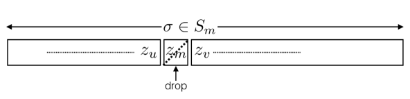
Figure 6: Crafting from $\sigma\in S_{m}$ a subset of $m-1$ reals for which the induction hypothesis can be applied in the proof of Lemma 7 (see text).

Let us drop the iteration index, thus letting $z_{i}\stackrel{{\scriptstyle\mathrm{.}}}{{=}}z_{Ti}$ for $i=0,1,...,m+1$ (with $z_{0}\stackrel{{\scriptstyle\mathrm{.}}}{{=}}z_{T\mbox{\tiny{{min}}}}$ and $z_{m+1}\stackrel{{\scriptstyle\mathrm{.}}}{{=}}z_{T\mbox{\tiny{{max}}}}$). We thus have $z_{i}\leq z_{i+1},\forall i$. We now pick one specific element in $\mathcal{U}(\bm{w},S)$, such that

$$u(z_{i}) = (-\underline{L}^{\prime})^{-1}(z_{i}),$$ (163)

for $i\in[d]$, which complies with the definition of $\mathcal{U}$ as both $u$ and $(-\underline{L}^{\prime})^{-1}$ are non decreasing. We then have

$$\int_{z_{1}}^{z_{m}}|(-\underline{L}^{\prime})^{-1}(z)-u(z)|\mathrm{d}z = \sum_{i=1}^{m-1}\int_{z_{i}}^{z_{i+1}}|(-\underline{L}^{\prime})^{-1}(z)-u(z)|\mathrm{d}z$$ (164)

$$\leq \sum_{i=1}^{m-1}(u(z_{i+1})-u(z_{i}))(z_{i+1}-z_{i})$$

$$\leq N\sum_{i=1}^{m-1}(z_{i+1}-z_{i})^{2},$$

where the first inequality holds because of (163) and $u$ is non decreasing, and the second inequality holds because of the constraint in Step 3. Let $S_{m}\ni\sigma:[m]\rightarrow[m]$ be a permutation of the indices. We now show

$$\sum_{i=1}^{m-1}(z_{\sigma(i+1)}-z_{\sigma(i)})^{2} \geq \sum_{i=1}^{m-1}(z_{i+1}-z_{i})^{2},\forall m>1,\forall\sigma\in S_{m}.$$ (165)

We show this by induction on $m$. The result is trivially true for $m=2$. Considering any $m>2$ and any permutation $\sigma\in S_{m}$, suppose the order of the $z$s in the permutation is as in Figure 6. Let $\Sigma_{\mathrm{tot}}\stackrel{{\scriptstyle\mathrm{.}}}{{=}}\sum_{i=1}^{m-1}(z_{\sigma(i+1)}-z_{\sigma(i)})^{2}$, which therefore includes term $(z_{m}-z_{u})^{2}+(z_{v}-z_{m})^{2}$. Now, drop $z_{m}$. This gives us a partial sum, $\Sigma_{\mathrm{partial}}$, over $\{z_{1},z_{2},...,z_{m-1}\}$ described by a permutation $\sigma\in S_{m-1}$ for which the induction hypothesis applies. We then have two cases:
Case 1: $1<\sigma(m)<m$, which implies that $z_{m}$ is "inside" the ordering given by $\sigma$ and is in fact the case depicted in Figure 6. In this case and using notations from Figure 6, we get:

$$\Sigma_{\mathrm{tot}} = \Sigma_{\mathrm{partial}}+(z_{m}-z_{u})^{2}+(z_{v}-z_{m})^{2}-(z_{v}-z_{u})^{2},$$ (166)

and the induction hypothesis yields

$$\Sigma_{\mathrm{partial}} \geq \sum_{i=1}^{m-2}(z_{i+1}-z_{i})^{2}.$$ (167)

So to show (165) we just need to show

$$\underbrace{\sum_{i=1}^{m-2}(z_{i+1}-z_{i})^{2}+(z_{m}-z_{u})^{2}+(z_{v}-z_{m})^{2}-(z_{v}-z_{u})^{2}}_{\mbox{Lowerbound on $\Sigma_{\mathrm{tot}}$ from \eqref{lbound1} and \eqref{lbound2}}} \geq \sum_{i=1}^{m-1}(z_{i+1}-z_{i})^{2},$$ (168)

which equivalently gives

$$(z_{m}-z_{u})^{2}+(z_{m}-z_{v})^{2} \geq (z_{v}-z_{u})^{2}+(z_{m}-z_{m-1})^{2}.$$ (169)

After putting $(z_{v}-z_{u})^{2}$ in the LHS and simplifying, we get equivalently that the induction holds if

$$2z_{m}^{2}-2z_{m}z_{u}-2z_{m}z_{v}+2z_{v}z_{u} \geq (z_{m}-z_{m-1})^{2}.$$ (170)

The LHS factorizes conveniently as $2z_{m}^{2}-2z_{m}z_{u}-2z_{m}z_{v}+2z_{v}z_{u}=2(z_{m}-z_{u})(z_{m}-z_{v})$. Since by hypothesis $z_{1}\leq z_{2}...\leq z_{m-1}\leq z_{m}$, we get $2(z_{m}-z_{u})(z_{m}-z_{v})\geq 2(z_{m}-z_{m-1})^{2}$, which implies (170) holds and the induction is proven.
Case 2: $\sigma(m)=m$ (the case $\sigma(m)=1$ give the same proof). In this case, $z_{m}$ is at the "right" of the permutation’s ordering. Using notations from Figure 6, we get in lieu of (166),

$$\Sigma_{\mathrm{tot}} = \Sigma_{\mathrm{partial}}+(z_{m}-z_{u})^{2},$$ (171)

and leaves us with the following result to show:

$$\sum_{i=1}^{m-2}(z_{i+1}-z_{i})^{2}+(z_{m}-z_{u})^{2} \geq \sum_{i=1}^{m-1}(z_{i+1}-z_{i})^{2},$$ (172)

which simplifies in $(z_{m}-z_{u})^{2}\geq(z_{m}-z_{m-1})^{2}$, which is true by assumption ($z_{u}\leq z_{m-1}\leq z_{m}$).

To summarize, we have shown that $\forall\sigma:[m]\rightarrow[m]$,

$$\int_{z_{1}}^{z_{m}}|(-\underline{L}^{\prime})^{-1}(z)-u(z)|\mathrm{d}z \leq \sum_{i=1}^{m-1}(z_{\sigma(i+1)}-z_{\sigma(i)})^{2}.$$ (173)

Assuming the $\varepsilon$-NN graph is 2-vertex-connected, we square the graph. Because of the triangle inequality on norm $\|.\|$, every edge has now length at most $2\varepsilon$ and the graph is Hamiltonian, a result known as Fleischner’s Theorem (Fleischner, 1974), (Gross & Yellen, 2004, p. 265, F17). Consider any Hamiltonian path and the permutation $\bm{\sigma}$ of $[m]$ it induces. We thus get $\|\bm{x}_{\sigma(i+1)}-\bm{x}_{\sigma(i)}\|\leq 2\varepsilon,\forall i$, and so Cauchy-Schwarz inequality yields:

$$\sum_{i=1}^{m-1}(z_{\sigma(i+1)}-z_{\sigma(i)})^{2} \stackrel{{\scriptstyle\mathrm{.}}}{{=}} \sum_{i=1}^{m-1}(\bm{w}^{\top}\bm{x}_{\sigma(i+1)}-\bm{w}^{\top}\bm{x}_{\sigma(i)})^{2}$$ (174)

$$\leq \|\bm{w}\|_{*}^{2}\sum_{i=1}^{m-1}\|\bm{x}_{\sigma(i+1)}-\bm{x}_{\sigma(i)}\|^{2}$$

$$\leq 2m\varepsilon^{2}\cdot\|\bm{w}\|_{*}^{2},$$

as claimed, where $\|.\|_{*}$ is the dual norm of $\|.\|$. We assemble (164) and (174) and get:

$$\int_{z_{1}}^{z_{m}}|(-\underline{L}^{\prime})^{-1}(z)-u(z)|\mathrm{d}z \leq 2Nm\varepsilon^{2}\cdot\|\bm{w}\|_{*}^{2},$$

which is the statement of the Lemma.

Remark: had we measured the $\ell_{1}$ discrepancy using the loss and not its link (and adding a second order differentiability condition), we could have used the fact that a Bregman divergence between two points is proportional to the square loss to get a result similar to the Lemma (see Section 8).

References

- Amari & Nagaoka (2000) Amari, S.-I. and Nagaoka, H. Methods of Information Geometry. Oxford University Press, 2000.
- Auer et al. (1995) Auer, P., Herbster, M., and Warmuth, M. Exponentially many local minima for single neurons. In NIPS*8, pp. 316–322, 1995.
- Azoury & Warmuth (2001) Azoury, K. S. and Warmuth, M. K. Relative loss bounds for on-line density estimation with the exponential family of distributions. MLJ, 43(3):211–246, 2001.
- Banerjee et al. (2004) Banerjee, A., Merugu, S., Dhillon, I., and Ghosh, J. Clustering with bregman divergences. In Proc. of the SIAM International Conference on Data Mining, pp. 234–245, 2004.
- Banerjee et al. (2005) Banerjee, A., Guo, X., and Wang, H. On the optimality of conditional expectation as a bregman predictor. IEEE Trans. IT, 51:2664–2669, 2005.
- Bartlett & Mendelson (2002) Bartlett, P.-L. and Mendelson, S. Rademacher and gaussian complexities: Risk bounds and structural results. JMLR, 3:463–482, 2002.
- Boissonnat et al. (2010) Boissonnat, J.-D., Nielsen, F., and Nock, R. Bregman voronoi diagrams. DCG, 44(2):281–307, 2010.
- Bousquet et al. (2019) Bousquet, O., Kane, D., and Moran, S. The optimal approximation factor in density estimation. In COLT’19, pp. 318–341, 2019.
- Boyd & Vandenberghe (2004) Boyd, S. and Vandenberghe, L. Convex optimization. Cambridge University Press, 2004.
- Bregman (1967) Bregman, L. M. The relaxation method of finding the common point of convex sets and its application to the solution of problems in convex programming. USSR Comp. Math. and Math. Phys., 7:200–217, 1967.
- Buja et al. (2005) Buja, A., Stuetzle, W., and Shen, Y. Loss functions for binary class probability estimation ans classification: structure and applications, 2005. Technical Report, University of Pennsylvania.
- Cranko et al. (2019) Cranko, Z., Menon, A.-K., Nock, R., Ong, C. S., Shi, Z., and Walder, C.-J. Monge blunts Bayes: Hardness results for adversarial training. In 36th ICML, pp. 1406–1415, 2019.
- de Finetti (1949) de Finetti, B. Rôle et domaine d’application du théorème de Bayes selon les différents points de vue sur les probabilités (in French). In 18th International Congress on the Philosophy of Sciences, pp. 67–82, 1949.
- Fleischner (1974) Fleischner, H. The square of every two-connected graph is Hamiltonian. Journal of Combinatorial Theory, Series B, 16:29–34, 1974.
- Grabocka et al. (2019) Grabocka, J., Scholz, R., and Schmidt-Thieme, L. Learning surrogate losses. CoRR, abs/1905.10108, 2019.
- Gross & Yellen (2004) Gross, J.-L. and Yellen, J. Handbook of graph theory. CRC press, 2004. ISBN 1-58488-090-2.
- Helmbold et al. (1995) Helmbold, D.-P., Kivinen, J., and Warmuth, M.-K. Worst-case loss bounds for single neurons. In NIPS*8, pp. 309–315, 1995.
- Herbster & Warmuth (1998) Herbster, M. and Warmuth, M. Tracking the best regressor. In 9 COLT, pp. 24–31, 1998.
- Kakade et al. (2011) Kakade, S., Kalai, A.-T., Kanade, V., and Shamir, O. Efficient learning of generalized linear and single index models with isotonic regression. In NIPS*24, pp. 927–935, 2011.
- Kearns & Vazirani (1994) Kearns, M. J. and Vazirani, U. V. An Introduction to Computational Learning Theory. M.I.T. Press, 1994.
- Liu et al. (2019) Liu, L., Wang, M., and Deng, J. UniLoss: Unified surrogate loss by adaptive interpolation. https://openreview.net/forum?id=ryegXAVKDB, 2019.
- Magdalou & Nock (2011) Magdalou, B. and Nock, R. Income distributions and decomposable divergence measures. Journal of Economic Theory, 146(6):2440–2454, 2011.
- Mei & Moura (2018) Mei, J. and Moura, J.-M.-F. SILVar: Single index latent variable models. IEEE Trans. Signal Processing, 66(11):2790–2803, 2018.
- Nock & Nielsen (2008) Nock, R. and Nielsen, F. On the efficient minimization of classification-calibrated surrogates. In NIPS*21, pp. 1201–1208, 2008.
- Nock & Nielsen (2009) Nock, R. and Nielsen, F. Bregman divergences and surrogates for learning. IEEE Trans.PAMI, 31:2048–2059, 2009.
- Nock & Williamson (2019) Nock, R. and Williamson, R.-C. Lossless or quantized boosting with integer arithmetic. In 36th ICML, pp. 4829–4838, 2019.
- Nock et al. (2008) Nock, R., Luosto, P., and Kivinen, J. Mixed Bregman clustering with approximation guarantees. In Proc. of the 19 ECML, pp. 154–169, 2008.
- Nock et al. (2016) Nock, R., Menon, A.-K., and Ong, C.-S. A scaled Bregman theorem with applications. In NIPS*29, pp. 19–27, 2016.
- Patrini et al. (2014) Patrini, G., Nock, R., Rivera, P., and Caetano, T. (Almost) no label no cry. In NIPS*27, 2014.
- Reid & Williamson (2010) Reid, M.-D. and Williamson, R.-C. Composite binary losses. JMLR, 11:2387–2422, 2010.
- Savage (1971) Savage, L.-J. Elicitation of personal probabilities and expectations. J. of the Am. Stat. Assoc., 66:783–801, 1971.
- Shorrocks (1980) Shorrocks, A.-F. The class of additively decomposable inequality measures. Econometrica, 48:613–625, 1980.
- Shuford et al. (1966) Shuford, E., Albert, A., and Massengil, H.-E. Admissible probability measurement procedures. Psychometrika, pp. 125–145, 1966.
- Siahkamari et al. (2019) Siahkamari, A., Saligrama, V., Castanon, D., and Kulis, B. Learning Bregman divergences. CoRR, abs/1905.11545, 2019.
- Streeter (2019) Streeter, M. Learning effective loss functions efficiently. CoRR, abs/1907.00103, 2019.
- Sypherd et al. (2019) Sypherd, T., Diaz, M., Laddha, H., Sankar, L., Kairouz, P., and Dasarathy, G. A tunable loss function for classification. CoRR, abs/1906.02314, 2019.
- Valiant (1984) Valiant, L. G. A theory of the learnable. Communications of the ACM, 27:1134–1142, 1984.
- Zhang (2004) Zhang, T. Statistical behaviour and consistency of classification methods based on convex risk minimization. Annals of Mathematical Statistics, 32:56––134, 2004.