Non-perturbative renormalization of the average color charge and multi-point correlators of color charge from a non-Gaussian small-$x$ action

Abstract

The McLerran-Venugopalan (MV) model is a Gaussian effective theory of color charge fluctuations at small-$x$ in the limit of large valence charge density, i.e., a large nucleus made of uncorrelated color charges. In this work, we explore the effects of the first non-trivial (even C-parity) non-Gaussian correction on the color charge density to the MV model (“quartic” term) in SU(2) and SU(3) color group in the non-perturbative regime. We compare our (numerical) non-perturbative results to (analytical) perturbative ones in the limit of small or large non-Gaussian fluctuations. The couplings in the non-Gaussian action, $\bar{\mu}$ for the quadratic and $\kappa_{4}$ for the quartic term, need to be renormalized in order to match the two-point function in the Gaussian theory. We investigate three different choices for the renormalization of these couplings: i) $\kappa_{4}$ is proportional to a power of $\bar{\mu}$; ii) $\kappa_{4}$ is kept constant and iii) $\bar{\mu}$ is kept constant. We find that the first two choices lead to a scenario where the small-$x$ action evolves towards a theory dominated by large non-Gaussian fluctuations, regardless of the system size, while the last one allows for controlling the deviations from the MV model.

I Introduction

As dynamic emission of soft gluons (over-)populates the phase space at high energies, hadrons may be described as a classical system. Such description is provided by the Color Glass Condensate (CGC) effective field theory CGC.review.new ; CGC.effective.theory , where calculations rely on a scale separation: large-$x$ (“valence”) partons act as a randomly distributed static color sources $\rho$ that generate the dynamical, short-lived, small-$x$ gluons. Due to the stochastic nature of the color charges, the resulting small-$x$ field, obtained by solving Classical Yang-Mills equations for a particular source configuration, must be averaged over a given ensemble $W_{Y}[\rho]$ of color charges. Therefore, any quantity of interest is obtained as the following expectation value,

$$\langle\mathcal{O}[\rho]\rangle_{Y}=\frac{\int[d\rho]\,W_{Y}[\rho]\,\mathcal{O}[\rho]}{\int[d\rho]W_{Y}[\rho]}\,,$$ (1)

where $Y=\log(x_{0}/x)$, with $x_{0}\sim 0.01$, denotes the rapidity variable.

Quantum corrections for $\langle\mathcal{O}[\rho]\rangle_{Y}$ due to the evolution in rapidity/energy are taken into account via the Wilsonian renormalization group equation for $W_{Y}[\rho]$ known as JIMWLK equation JalilianMarian:1996xn ; JalilianMarian:1997jx ; JalilianMarian:1997gr ; JalilianMarian:1997dw ; JalilianMarian:1998cb ; Kovner:1999bj ; Kovner:2000pt ; Iancu:2000hn ; Iancu:2001ad ; Ferreiro:2001qy . Solving such an evolution equation is an initial value problem; it requires an initial distribution of color charges as input. For an infinitely large nucleus made of uncorrelated color charges, it is possible to show that $W_{0}[\rho]$ is a Gaussian, which is known as the McLerran-Venugopalan (MV) model CGC.Raju.McLerran , and it is widely employed in CGC calculations.

In reality, however, the number of color charges is finite and their distribution should deviate from a Normal one. Such deviation should occur even in the absence of quantum corrections and also for large nuclei Lam:2001ax , as the finiteness of color charges by itself introduce correlations. Therefore, the initial condition for the evolution equation is not necessarily a Gaussian. It is known that a Gaussian distribution is not a solution of the JIMWLK evolution equation JalilianMarian:1997gr , and the small-$x$ evolution generates non-quadratic terms (in the color charge $\rho$) even if one starts with a Gaussian distribution of color charges. Non-Gaussian contributions were indirectly studied within JIMWLK evolution. Starting with a Gaussian initial condition (MV model), it was found that the small-$x$ evolution appears to preserve the Gaussianity of the initial color charge distribution for two specific configurations (“line” and “square” configurations) of the correlator of four Wilson lines in Dumitru:2011vk . At the same time, the product of the correlator of two and four Wilson lines, which is present in the cross-section for di-hadron production in proton-nucleus collisions Marquet:2007vb , has shown deviations from analytical expressions obtained in the Gaussian approximation Dominguez:2011wm in the saturation region. It is still unknown what happens if one starts the evolution with a non-Gaussian initial condition instead of considering the MV model. It was pointed out in Lappi:2015vta that the small-$x$ evolution may introduce non-Gaussian contributions in some observables such as the azimuthal anisotropies, $v_{n}$.

Corrections to the MV model for SU(3) color group have already been calculated in the literature Jeon:2004rk ; Dumitru:2011zz up to the fourth-order in the color charges. The resulting non-Gaussian weight function has then been used to perform perturbative calculations in the dilute regime Dumitru:2011zz ; Dumitru:2011ax ; Dumitru:2012tw , where the corrections to the MV model are assumed to be small. The impact of a non-Gaussian weight function on observables has not been investigated in details yet, but it is expected that it could lead to a better representation of the initial conditions for proton-proton and proton-nucleus collisions. Moreover, such higher-order terms may contribute to experimental observables in different physical processes, such as multi-particle correlations in nuclear collisions Dumitru:2011zz ; Kovner:2010xk , di-jets produced in proton-proton and proton-nucleus Marquet:2007vb ; Dominguez:2011wm and inclusive Deep Inelastic Scattering structure functions, $F_{L}$ and $F_{2}$, which can be related to the forward scattering amplitude of a quark-antiquark pair GolecBiernat:1998js .

In this work, we present a first study of the effects of non-Gaussian corrections to the MV model on multi-point correlations of color charges in the fully non-perturbative regime. Specifically, we investigate three different renormalization schemes for determining the couplings of the non-Gaussian small-$x$ action. Our calculations will be done in lattice regularization and carried out for $Y=0$; therefore, they may be used as initial conditions for the renormalization group equations to go beyond the Gaussian approximation in the CGC effective theory. We shall show below that one of these renormalization schemes allows us to control the deviations from the MV model as one approaches the continuum while the other two lead to a small-$x$ action that evolves towards a theory dominated by strong non-Gaussian fluctuations regardless of the system size.

In the next section, we briefly present the Gaussian and non-Gaussian effective weight functions which are used to take an average over the color sources in the CGC approach. We then present perturbative results in the limit of small as well as large non-Gaussian fluctuations, and compare them to non-perturbative calculations, which includes all orders of $1/\kappa_{4}$ (see Eq. (3) for the definition of $\kappa_{4}$).

II Weight functions for color charge average

The central limit theorem applies in the high density limit for color charge density and the absence of correlations between color charges at different coordinates Lam:2001ax . Then, $W[\rho]$ is given by the MV model CGC.Raju.McLerran

$$W_{MV}[\rho_{x_{\perp}}]=\exp\bigg{\{}-\int\,d^{2}{x_{\perp}}{\delta^{ab}\,\rho^{a}_{x_{\perp}}\rho^{b}_{x_{\perp}}\over 2\mu^{2}}\bigg{\}}~{},$$ (2)

where $\mu^{2}$ represents the average color charge squared per unit area per color degree of freedom, and $\rho^{i}_{{x_{\perp}}}\equiv\rho^{i}({x_{\perp}})$ is the color charge density at a given transverse coordinate $x_{\perp}$. In this case, the two-point function of color charge density is the only non-trivial correlator: any higher-order $n$-point function ($n=4,6,8...$) can be factorized into a product of $n/2$ two-point functions.

We shall consider deviations from a Gaussian weight due to finite number of color sources. Non-Gaussian corrections to Eq. (2) for SU($N_{c}$) color group, where $N_{c}\leqslant 3$, have been calculated in the literature Jeon:2004rk ; Dumitru:2011zz up to the forth-order in the color charges:

$$W[\rho_{x_{\perp}}] \simeq \exp\bigg{\{}-\int\,d^{2}x_{\perp}\bigg{[}{\delta^{ab}\,\rho^{a}_{x_{\perp}}\rho^{b}_{x_{\perp}}\over 2{\bar{\mu}}^{2}}-{d^{abc}\,\rho^{a}_{x_{\perp}}\rho^{b}_{x_{\perp}}\rho^{c}_{x_{\perp}}\over\kappa_{3}}+{\delta^{ab}\delta^{cd}+\delta^{ac}\delta^{bd}+\delta^{ad}\delta^{bc}\over\kappa_{4}}\rho^{a}_{x_{\perp}}\rho^{b}_{x_{\perp}}\rho^{c}_{x_{\perp}}\rho^{d}_{x_{\perp}}\bigg{]}\bigg{\}}$$ (3)

$$= \exp\bigg{\{}-\int\,d^{2}x_{\perp}\bigg{[}{\rho^{a}_{x_{\perp}}\rho^{a}_{x_{\perp}}\over 2{\bar{\mu}}^{2}}-{d^{abc}\,\rho^{a}_{x_{\perp}}\rho^{b}_{x_{\perp}}\rho^{c}_{x_{\perp}}\over\kappa_{3}}+{3\over\kappa_{4}}\rho^{a}_{x_{\perp}}\rho^{a}_{x_{\perp}}\rho^{b}_{x_{\perp}}\rho^{b}_{x_{\perp}}\bigg{]}\bigg{\}}\,,$$

where $\delta^{ij}$ is the Kronecker’s delta, $d^{abc}$ is the symmetric tensor in the SU(3) Lie algebra Jeon:2004rk and $\bar{\mu}^{2}$ is the average color charge squared, $\kappa_{3}$ and $\kappa_{4}$ represent the couplings from the first odd C-parity (“cubic” term) and even C-parity (“quartic” term) corrections to the MV model. When non-Gaussian corrections to the MV model are small, the couplings in Eq. (3) can be written as Dumitru:2011zz :

$$\bar{\mu}^{2}\equiv{g^{2}A\over 2\pi R^{2}}\,,\qquad\qquad\kappa_{3}\equiv 3{g^{3}A^{2}\over(\pi R^{2})^{2}}\,={12\bar{\mu}^{4}\over g}\,,\qquad\qquad\kappa_{4}\equiv 18{g^{4}A^{3}\over(\pi R^{2})^{3}}\,={144\bar{\mu}^{6}\over g^{2}}\,,$$ (4)

where $A$ represents the mass number and $R$ the radius of the system of interest. For SU(2), $\kappa_{4}$ is given by

$$\kappa_{4}\equiv 6{g^{4}A^{3}\over(\pi R^{2})^{3}}\,={48\bar{\mu}^{6}\over g^{2}}.$$ (5)

The factor in Eq. (5) can be verified in two different ways: by following the calculation in Jeon:2004rk but including higher-order contributions in the Taylor expansion of $G_{k:s}$ in their Eq. (19) and by writing the quartic Casimir in Eq. (12) of Dumitru:2011zz for SU(2). We note that the small-$x$ action for SU(2) symmetry group does not have cubic (“odderon”) term as the symbol $d^{abc}$ is zero.

In what follows, we only consider the quartic term in the SU(3) case, leaving the study of the cubic term in the future. While corrections (at perturbative level) due to the inclusion of the cubic term are expected at order $1/\kappa_{3}^{2}$ for SU(3) Dumitru:2011zz , our results for SU(2) are exact up to all orders in $1/\kappa_{4}$.

The coupling in the quadratic and the quartic term in Eq. (3), $\bar{\mu}$ and $\kappa_{4}$, are not chosen freely. It is required that the inclusion of non-Gaussian corrections does not impact any quantity depending solely on the correlator of two-color charges, $\langle\rho^{a}_{x_{\perp}}\rho^{b}_{y_{\perp}}\rangle$, since this is a quantity determined by the quadratic part of the small-$x$ action. Thus, one needs to renormalize the couplings in the non-Gaussian action to match the two-point function of color charges from the Gaussian theory. In this way, the two couplings are related to each other and one more condition is needed to uniquely fix them. We consider three possible ways to fix these couplings. One option is to keep $\kappa_{4}/\bar{\mu}^{6}\equiv\lambda$ constant. In principle, $\lambda$ can be fixed to any (positive) value. Motivated by the expression for $\bar{\mu}^{2}$ in Eq. (4), we take $\lambda=\gamma/g^{2}$, where $\gamma=48\,(144)$ for SU(2) (SU(3)). A second option is to keep $\kappa_{4}$ constant. The parametric dependence shown in Eq. (4) and Eq. (5) is no longer valid in this renormalization scheme. The third option is to control the deviation from the MV model by fixing the parameter $Z$ defined by

$$Z=\frac{\mu^{2}}{\bar{\mu}^{2}}\,.$$ (6)

We shall show that the first two renormalization schemes lead to a theory dominated by non-Gaussian fluctuations independent of the system size.

III (Semi-)Analytical results for color average in the transverse lattice

This section presents the expressions for the correlators of two- and four-color charges for different approximations. The first approximation is to assume that the quartic term in Eq. (3) is small Dumitru:2011zz . The second considers a limit of large non-Gaussian corrections, in which the quartic term is large. Otherwise stated, all expressions will be presented in lattice regularization by approximating the two-dimensional transverse space by $N_{s}^{2}$ lattice sites with lattice spacing $\mathtt{a}$.

For a weight function which only involves the product of square power of color charges, as in the case for SU(2) and SU(3) without the cubic term, one can calculate the color average in Eq. (1) on a lattice by evaluating

$$\langle\mathcal{O}\rangle=\frac{\int(\prod_{x}\prod_{a}d\rho^{a}_{x})\,\mathcal{O}\,e^{-\sum_{y}W_{y}}}{\int(\prod_{x}\,\prod_{a}d\rho^{a}_{x})\,e^{-\sum_{y}W_{y}}}=\frac{\int(\prod_{a}d\rho^{a}_{x})\,\mathcal{O}_{x}\,e^{-W_{x}}}{\int(\prod_{a}d\rho^{a}_{x})\,e^{-W_{x}}}\,=\frac{\int dr\,r^{N_{c}^{2}-2}\,\mathcal{O}_{r}\,e^{-W_{r}}}{\int dr\,r^{N_{c}^{2}-2}\,e^{-W_{r}}}\,,$$ (7)

where $W_{r}$ is defined as

$$W_{r}=\frac{a^{2}r^{2}}{2\bar{\mu}^{2}}+\frac{3a^{2}r^{4}}{\kappa_{4}}\,.$$ (8)

The second equality in Eq. (7) is obtained by assuming that $\mathcal{O}$ is a local operator. As discussed below, the correlators of two- and four-color charges will be affected by non-Gaussian corrections when calculated locally. In such configuration, the functional integral becomes an integral over the color charges at a single site. The rightmost result is then obtained after using spherical coordinates in $N_{c}^{2}-1$ dimensions, which factor out any angular dependencies.

The requirement that any quantity depending only on the two-point function of color charges remains unchanged introduces the following constraint

$$\langle\rho^{a}_{x}\rho^{b}_{y}\rangle_{\text{non-Gaussian}}=\langle\rho^{a}_{x}\rho^{b}_{y}\rangle_{\text{MV model}}=\frac{\delta^{ab}\delta_{xy}}{\mathtt{a}^{2}}\mu^{2}\,,$$ (9)

where $\mathtt{a}^{2}$ represents the area of a lattice cell, $x$ and $y$ are discrete points in the transverse lattice, and $\delta_{xy}/{\mathtt{a}^{2}}$ is the lattice counterpart of the Dirac’s delta, $\delta(x-y)$; from here on, we use the shorthand notation “NG” to denote results obtained using the non-Gaussian weight function. Thus, one of the couplings in the non-Gaussian weight function is chosen in order to satisfy Eq. (9).

As noted above, local operators do not present a spatial dependence over a two-dimensional lattice and the integral is only over the color space. Then the correlator of two-color charges (${\mathcal{O}}_{x}=\rho_{x}^{a}\rho_{y}^{b}$) is given by

$$\langle\rho^{a}_{x}\rho^{b}_{y}\rangle_{\text{NG}}=\delta^{ab}\delta_{xy}\,\frac{\mu^{2}\sqrt{X}}{Z\,a^{2}}\frac{U\left(\frac{1}{4}\left(N_{c}^{2}+1\right),\frac{1}{2},X\right)}{U\left(\frac{1}{4}\left(N_{c}^{2}-1\right),\frac{1}{2},X\right)}=\delta^{ab}\delta_{xy}\,\frac{\sqrt{\kappa_{4}}}{4\,\sqrt{3}\,a}\frac{U\left(\frac{1}{4}\left(N_{c}^{2}+1\right),\frac{1}{2},X\right)}{U\left(\frac{1}{4}\left(N_{c}^{2}-1\right),\frac{1}{2},X\right)}$$ (10)

where $X=a^{2}\,\kappa_{4}/48\bar{\mu}^{4}$ and

$$U(\alpha,\beta,\omega)=\frac{1}{\Gamma(\alpha)}\int_{0}^{\infty}e^{-\omega t}\,t^{\alpha-1}\,(1+t)^{\beta-\alpha-1}\,dt$$ (11)

denotes the Tricomi’s confluent hypergeometric function; $\Gamma(\alpha)$ is the Gamma function. The condition Eq. (9) for SU($N_{c}$) is given by

$$\frac{\bar{\mu}^{2}\sqrt{X}}{a^{2}}\frac{U\left(\frac{1}{4}\left(N_{c}^{2}+1\right),\frac{1}{2},X\right)}{U\left(\frac{1}{4}\left(N_{c}^{2}-1\right),\frac{1}{2},X\right)}=\frac{\mu^{2}}{\mathtt{a}^{2}}\,.$$ (12)

The four-point function of color charges can also be expressed in terms of the Tricomi’s confluent hypergeometric function:

$$\langle\rho^{a}_{x}\rho^{a}_{x}\rho^{c}_{x}\rho^{c}_{x}\rangle_{\text{NG}}=\left(N_{c}^{4}-1\right)\,\frac{\bar{\mu}^{4}}{a^{4}}\frac{XU\left(\frac{1}{4}\left(N_{c}^{2}+3\right),\frac{1}{2},X\right)}{U\left(\frac{1}{4}\left(N_{c}^{2}-1\right),\frac{1}{2},X\right)}\,.$$ (13)

We finish this section by summarizing the four-point function of color charges, $\langle\rho_{x}^{a}\rho_{y}^{b}\rho_{u}^{c}\rho_{v}^{d}\rangle$ in the MV model. Calculating the color average in Eq. (7) with the Gaussian ensemble results in

$$\langle\rho^{a}_{x}\rho^{b}_{y}\rho^{c}_{u}\rho^{d}_{v}\rangle_{\rm MV}=\mu^{4}\left[\,\delta^{ab}\delta^{cd}\delta(x-y)\delta(u-v)+\delta^{ac}\delta^{bd}\delta(x-u)\delta(y-v)+\delta^{ad}\delta^{bc}\delta(x-v)\delta(y-u)\,\right]\,.$$ (14)

We point out that the color factor multiplying $\mu^{4}$ is dependent on the configuration. We have a factorizable configuration in the lattice configuration that each pair of color charges sit at different sites (i.e. $x=y$, $u=v$ but $x\neq u$). Each one of the two-point function contributes with a factor of $N_{c}^{2}-1$ after contracting color indexes. The coefficient of the correlator of four-color charges then evaluates to

$$\langle\rho_{x}^{a}\rho_{x}^{a}\rho_{u}^{c}\rho_{u}^{c}\rangle_{\rm MV}=\langle\rho_{x}^{a}\rho_{x}^{a}\rangle\langle\rho_{u}^{c}\rho_{u}^{c}\rangle=(N_{c}^{2}-1)^{2}\,\frac{\mu^{4}}{a^{4}}\,.$$ (15)

On the other hand, in the lattice configuration where $x=y=u=v$, the coefficient of the correlator is given by

$$\langle\rho_{x}^{a}\rho_{x}^{a}\rho_{x}^{c}\rho_{x}^{c}\rangle_{\rm MV}=\left[(N_{c}^{2}-1)^{2}+2(N_{c}^{2}-1)\right]\frac{\mu^{4}}{a^{4}}=(N_{c}^{4}-1)\,\frac{\mu^{4}}{a^{4}}\,,$$ (16)

having a different color factor from the factorizable case.

In the next section, we shall consider the Taylor expansion of the hypergeometric functions in two different regimes in order to study the limit of small as well as large non-Gaussian fluctuations. The results from these asymptotic cases will be compared to non-perturbative numerical calculations.

III.1 The dilute regime: quartic term as small perturbation

In the $\kappa_{4}\to\infty$ limit the quartic term is a small perturbation. Expanding Eq. (12) at $X\to\infty$ up to the order of $1/X$:

$$\bar{\mu}^{2}\left(1-\frac{N_{c}^{2}+1}{4X}\right)=\mu^{2}\,.$$ (17)

Writing it in terms of $\kappa_{4}$ gives:

$$\mu^{2}=\bar{\mu}^{2}\left(1-12\frac{\bar{\mu}^{4}}{\kappa_{4}}\frac{(N_{c}^{2}+1)}{\mathtt{a}^{2}}\right)=\bar{\mu}^{2}\,Z\,,$$ (18)

which is the same result obtained after a perturbative expansion of the quartic term in the small-$x$ action as done in Ref. Dumitru:2011zz .

According to Dumitru:2011zz , a contribution of order $1/\kappa_{4}^{2}$ renormalizes the $\bar{\mu}^{8}$ factor appearing in the correction to the four-point function of color charges at order $1/\kappa_{4}$. Expanding Eq. (13) at $X\to\infty$ up to the term $1/X^{2}$ yields

$$\langle\rho^{a}_{x}\rho^{a}_{x}\rho^{c}_{x}\rho^{c}_{x}\rangle_{\text{NG}} \simeq(N_{c}^{4}-1)\frac{\bar{\mu}^{4}}{a^{4}}\left[1-\frac{N_{c}^{2}+2}{2X}+\frac{31+24N_{c}^{2}+5N_{c}^{4}}{16X^{2}}\right]$$ (19)

$$=(N_{c}^{4}-1)\frac{\bar{\mu}^{4}}{a^{4}}\left[1-\frac{N_{c}^{2}+1}{2X}-\frac{1}{2X}\left(1-\frac{N_{c}^{2}+1}{X}\right)+\frac{23+16N_{c}^{2}+5N_{c}^{4}}{16X^{2}}\right]\,.$$ (20)

We renormalize $\bar{\mu}^{4}$ and $\bar{\mu}^{8}$ by using Eq. (17):

$$\mu^{4}\simeq\bar{\mu}^{4}\left(1-\frac{N_{c}^{2}+1}{2X}\right),~{}~{}~{}\mu^{8}\simeq\bar{\mu}^{8}\left(1-\frac{N_{c}^{2}+1}{X}\right)\,,$$ (21)

valid at order $1/\kappa_{4}$. The remaining terms of order $1/\kappa_{4}^{2}$ in Eq. (20) are discarded, as in Dumitru:2011zz . Then, we obtain the correlator of four-color charges in the dilute limit up to the order of $\kappa_{4}$ Dumitru:2011zz :

$$\langle\rho^{a}_{x}\rho^{a}_{y}\rho^{c}_{u}\rho^{c}_{v}\rangle_{\text{NG}}=(N_{c}^{4}-1)\,\mu^{4}\bigg{[}\frac{\delta_{xy}}{a^{2}}\frac{\delta_{uv}}{a^{2}}\left(1-24\frac{\mu^{4}}{\kappa_{4}}\frac{\delta_{xu}}{a^{2}}\right)+\frac{\delta_{xu}}{a^{2}}\frac{\delta_{yv}}{a^{2}}\left(1-24\frac{\mu^{4}}{\kappa_{4}}\frac{\delta_{xy}}{a^{2}}\right)+\frac{\delta_{xv}}{a^{2}}\frac{\delta_{yu}}{a^{2}}\left(1-24\frac{\mu^{4}}{\kappa_{4}}\frac{\delta_{xy}}{a^{2}}\right)\bigg{]}\,.$$ (22)

All other components are similar to this one, with the only difference being the permutation of the indexes of Kronecker’s deltas. In the continuum notation, it reads

$$\langle\rho^{a}_{x}\rho^{b}_{y}\rho^{c}_{u}\rho^{d}_{v}\rangle_{\text{NG}}= \mu^{4} \bigg{[}\delta^{ab}\delta^{cd}\delta(x-y)\delta(u-v)\left(1-24\frac{\mu^{4}}{\kappa_{4}}\delta(x-u)\right)+\delta^{ac}\delta^{bd}\delta(x-u)\delta(y-v)\left(1-24\frac{\mu^{4}}{\kappa_{4}}\delta(x-y)\right)$$ (23)

$$+ \delta^{ad}\delta^{bc}\delta(x-v)\delta(y-u)\left(1-24\frac{\mu^{4}}{\kappa_{4}}\delta(x-y)\right)\bigg{]}\,.$$

The combination of (Dirac’s) delta functions is such that the non-Gaussian correction modifies the result from the MV model only if the four-point function of color charges is a local quantity, that is, $x=y=u=v$. On the other hand, in the configuration that each pair of color charges sit at different sites (i.e. $x=y$, $u=v$ but $x\neq u$), the four-point function factorizes into the product of two two-point functions, and the result is identical to the one in the MV model.

Since we are interested in the effect of the non-Gaussian correction to the MV model, we set $x=y=u=v$ in the lattice expression; in other words, we calculate Eq. (22) at the delta functions. The ratio of the correlator of four-color charges in the non-Gaussian to the Gaussian theory results in:

$$\frac{\langle\rho^{a}_{x}\rho^{a}_{x}\rho^{c}_{x}\rho^{c}_{x}\rangle_{\text{NG}}}{\langle\rho^{a}_{x}\rho^{a}_{x}\rho^{c}_{x}\rho^{c}_{x}\rangle_{\rm MV}}=1-24\frac{\mu^{4}}{\kappa_{4}\,a^{2}}\,,$$ (24)

for the dilute limit.

III.2 Large non-Gaussian fluctuations

We now consider the limit of large non-Gaussian fluctuations, $Z\to 0$, where sizable deviations from the MV model are expected.

Taylor expanding the left-hand side of Eq. (12) around $X\rightarrow 0$ up to the order $\mathcal{O}[X]$ yields:

$$\frac{\mu^{2}}{Z\,a^{2}}\left[\frac{\Gamma\left(\frac{1}{4}\left(N_{c}^{2}+1\right)\right)}{\Gamma\left(\frac{1}{4}\left(N_{c}^{2}+3\right)\right)}\sqrt{X}+\left(\frac{2\Gamma\left(\frac{1}{4}\left(N_{c}^{2}+1\right)\right)^{2}}{\Gamma\left(\frac{1}{4}\left(N_{c}^{2}-1\right)\right)\Gamma\left(\frac{1}{4}\left(N_{c}^{2}+3\right)\right)}-2\right)X\right]=\frac{\mu^{2}}{\mathtt{a}^{2}}$$

Thus, the expression up to the order of $Z$ is given by

$$\frac{\Gamma\left(\frac{1}{4}\left(N_{c}^{2}+1\right)\right)}{4\,\sqrt{3}\,\Gamma\left(\frac{1}{4}\left(N_{c}^{2}+3\right)\right)}\frac{\sqrt{\kappa_{4}}}{a}+\left(\frac{\Gamma\left(\frac{1}{4}\left(N_{c}^{2}+1\right)\right)^{2}}{\Gamma\left(\frac{1}{4}\left(N_{c}^{2}-1\right)\right)\Gamma\left(\frac{1}{4}\left(N_{c}^{2}+3\right)\right)}-1\right)\frac{Z\,\kappa_{4}}{24\,\mu^{2}}=\frac{\mu^{2}}{\mathtt{a}^{2}}\,.$$ (25)

We will work out the solution of Eq. (25) for the three renormalization schemes in the next sections.

We now present an analytical expression for the local configuration $\langle\rho_{x}^{a}\rho_{x}^{b}\rho_{x}^{c}\rho_{x}^{d}\rangle$ in the regime of large non-Gaussian fluctuations. We begin by setting $x=y=u=v$, so that we calculate Eq. (7) for this particular configuration. For the color space, we have the following color contractions $\delta^{ab}\delta^{cd}+\delta^{ac}\delta^{bd}+\delta^{ad}\delta^{bc}$. It is sufficient to consider the case $a=b$ and $c=d$, as each term yields the same contribution. For the large non-Gaussian fluctuation limit, Taylor expanding Eq. (13) around $X\rightarrow 0$ up to the order $\mathcal{O}[Z^{2}]$ yields:

$$\langle\rho^{a}_{x}\rho^{a}_{x}\rho^{c}_{x}\rho^{c}_{x}\rangle_{\text{NG}} = (N_{c}^{4}-1)\,\bigg{[}\frac{\kappa_{4}}{12\,a^{2}\left(N_{c}^{2}+1\right)}-\frac{\sqrt{\pi}\,2^{(7-N_{c}^{2})/2}\,\Gamma\left(\frac{1}{2}\left(N_{c}^{2}+1\right)\right)}{3\,\sqrt{3}\,\left(N_{c}^{2}+1\right)\,\Gamma\left(\frac{1}{4}\left(N_{c}^{2}+3\right)\right)^{2}\,}\frac{Z\,\kappa_{4}^{3/2}}{a\,\mu^{2}}$$ (26)

$$+ \frac{\left(4\,\Gamma\left(\frac{1}{4}\left(N_{c}^{2}+3\right)\right)^{2}-\left(N_{c}^{2}-1\right)\,\Gamma\left(\frac{1}{4}\left(N_{c}^{2}+1\right)\right)^{2}\right)}{1152\left(N_{c}^{2}+1\right)\,\Gamma\left(\frac{1}{4}\left(N_{c}^{2}+3\right)\right)^{2}}\frac{Z^{2}\,\kappa_{4}^{2}}{\mu^{4}}\bigg{]}\,.$$

Let us now compute the four-point function of color charges in the lowest order. From Eq. (25), one obtains

$$\kappa_{4}=48\,\frac{\Gamma\left(\frac{1}{4}\left(N_{c}^{2}+3\right)\right)^{2}}{\Gamma\left(\frac{1}{4}\left(N_{c}^{2}+1\right)\right)^{2}}\frac{\mu^{4}}{a^{2}}\,.$$ (27)

We see that $\kappa_{4}$ does not depend on $\bar{\mu}$. For the four-point function of color charges in the leading order term in Eq. (26) results in

$$\langle\rho^{a}_{x}\rho^{a}_{x}\rho^{c}_{x}\rho^{c}_{x}\rangle_{\text{NG}}=\frac{(N_{c}^{4}-1)\,\kappa_{4}}{12\,a^{2}\,\left(N_{c}^{2}+1\right)}=\frac{4\left(N_{c}^{2}-1\right)\,\Gamma\left(\frac{1}{4}\left((N_{c}^{2}+3\right)\right)^{2}}{\Gamma\left(\frac{1}{4}\left((N_{c}^{2}+1\right)\right)^{2}}\frac{\mu^{4}}{a^{4}}=\frac{\left(N_{c}^{4}-1\right)\,\Gamma\left(\frac{1}{4}\left(N_{c}^{2}+3\right)\right)^{2}}{\Gamma\left(\frac{1}{4}\left(N_{c}^{2}+1\right)\right)\Gamma\left(\frac{1}{4}\left(N_{c}^{2}+5\right)\right)}\frac{\mu^{4}}{a^{4}}\,,$$ (28)

where we used $\Gamma((N_{c}^{2}+1)/4)=4\,\Gamma((N_{c}^{2}+5)/4)\,/\,(N_{c}^{2}+1)$.

The correlator of four-color charges in the non-Gaussian theory follows the same structure as Eq. (23) in continuum notation:

$$\langle\rho^{a}_{x}\rho^{b}_{y}\rho^{c}_{u}\rho^{d}_{v}\rangle_{\text{NG}} = \mu^{4}\bigg{\{}\delta^{ab}\delta^{cd}\delta(x-y)\delta(u-v)\left[1-{\mathcal{C}_{\mathrm{NG}}}\frac{\mu^{4}}{\kappa_{4}}\,\delta(x-u)\right]+\delta^{ac}\delta^{bd}\delta(x-u)\delta(y-v)\left[1-{\mathcal{C}_{\mathrm{NG}}}\frac{\mu^{4}}{\kappa_{4}}\,\delta(x-y)\right]$$ (29)

$$+ \delta^{ad}\delta^{bc}\delta(x-v)\delta(y-u)\left[1-{\mathcal{C}_{\mathrm{NG}}}\frac{\mu^{4}}{\kappa_{4}}\,\delta(x-y)\right]\bigg{\}}\,,$$

where ${\mathcal{C}_{\mathrm{NG}}}$ reads

$${\mathcal{C}_{\mathrm{NG}}}=48\frac{\Gamma(\frac{1}{4}(N_{c}^{2}+3))^{2}}{\Gamma(\frac{1}{4}(N_{c}^{2}+1))^{2}}\bigg{[}1-\frac{\Gamma\left(\frac{1}{4}\left(N_{c}^{2}+3\right)\right)^{2}}{\Gamma\left(\frac{1}{4}\left(N_{c}^{2}+1\right)\right)\Gamma\left(\frac{1}{4}\left(N_{c}^{2}+5\right)\right)}\bigg{]}\,.$$ (30)

As in the MV model, the color factor multiplying $\mu^{4}/{\mathtt{a}^{4}}$ depends on the spatial configuration in which the correlator is calculated:

$$\langle\rho^{a}_{x}\rho^{a}_{y}\rho^{c}_{u}\rho^{c}_{v}\rangle_{\text{NG}}\propto\,\,\,\begin{cases}(N_{c}^{2}-1)^{2}\,,&\text{if }x=y,\,\,u=v\,\,(u\neq x)\\ (N_{c}^{4}-1)\,\frac{\Gamma\left(\frac{1}{4}\left(N_{c}^{2}+3\right)\right)^{2}}{\Gamma\left(\frac{1}{4}\left(N_{c}^{2}+1\right)\right)\Gamma\left(\frac{1}{4}\left(N_{c}^{2}+5\right)\right)}\,,&\text{if }x=y=u=v\,.\end{cases}$$ (31)

We then consider the ratio of the correlator of four-color charges from the non-Gaussian to the Gaussian theories for the configurations shown above. When setting $x=y$, $u=v$ with the condition $u\neq x$ the non-Gaussian correction is not present, and we have

$$\frac{\langle\rho^{a}_{x}\rho^{a}_{x}\rho^{c}_{u}\rho^{c}_{u}\rangle_{\text{NG}}}{\langle\rho^{a}_{x}\rho^{a}_{x}\rho^{c}_{u}\rho^{c}_{u}\rangle_{\text{MV}}}=\frac{\langle\rho^{a}_{x}\rho^{a}_{x}\rangle\langle\rho^{c}_{u}\rho^{c}_{u}\rangle}{\langle\rho^{a}_{x}\rho^{a}_{x}\rangle\langle\rho^{c}_{u}\rho^{c}_{u}\rangle}=\frac{(N_{c}^{2}-1)^{2}\,\mu^{4}/a^{4}}{(N_{c}^{2}-1)^{2}\,\mu^{4}/a^{4}}=1\,,$$ (32)

as expected (see Eq. (15)). On the other hand, for the configuration where $x=y=u=v$, the ratio of $\langle\rho^{a}_{x}\rho^{a}_{x}\rho^{c}_{x}\rho^{c}_{x}\rangle$ from the non-Gaussian theory to the Gaussian theory yields:

$$\frac{\langle\rho^{a}_{x}\rho^{a}_{x}\rho^{c}_{x}\rho^{c}_{x}\rangle_{\text{NG}}}{\langle\rho^{a}_{x}\rho^{a}_{x}\rho^{c}_{x}\rho^{c}_{x}\rangle_{\text{MV}}}=\frac{\Gamma\left(\frac{1}{4}\left(N_{c}^{2}+3\right)\right)^{2}}{\Gamma\left(\frac{1}{4}\left(N_{c}^{2}+1\right)\right)\Gamma\left(\frac{1}{4}\left(N_{c}^{2}+5\right)\right)}\,,$$ (33)

showing that, in the $Z\rightarrow 0$ limit, the ratio of correlators of color charge depends only on the number of colors $N_{c}$ (so it is constant for fixed $N_{c}$). For SU(2) and SU(3), Eq. (33) evaluates to

$$0.822504$$ for SU(2) (34a)

$$0.905415 \quad\text{for SU(3)}\,,$$ (34b)

so the correlator of four-color charges calculated at the delta functions in a lattice setup should decrease by $\sim 18\%$ ($\sim 10\%$) in the non-Gaussian theory compared to the Gaussian theory for SU(2) (SU(3)) in the limit of very large non-Gaussian fluctuations.

Finally, we note that there exist two different conditions where one may factorize four-point functions (and other higher-order correlators) of color charges into products of two-point functions Dumitru:2010mv : when using a Gaussian weight function for color average, as the MV model, and the large-$N_{c}$ limit. For the large-$N_{c}$ limit in our case, the ratio Eq. (33) evaluates to one:

$$\lim\limits_{N_{c}\rightarrow\infty}\frac{\langle\rho^{a}_{x}\rho^{a}_{x}\rho^{c}_{x}\rho^{c}_{x}\rangle_{\text{NG}}}{\langle\rho^{a}_{x}\rho^{a}_{x}\rho^{c}_{x}\rho^{c}_{x}\rangle_{\text{MV}}}=\lim\limits_{N_{c}\rightarrow\infty}\frac{\Gamma\left(\frac{1}{4}\left(N_{c}^{2}+3\right)\right)^{2}}{\Gamma\left(\frac{1}{4}\left(N_{c}^{2}+1\right)\right)\Gamma\left(\frac{1}{4}\left(N_{c}^{2}+5\right)\right)}=1\,.$$ (35)

IV Renormalization schemes

In this section, we consider two opposite perturbative regimes, small and large non-Gaussian fluctuations, in three different renormalization schemes. These results are then compared to a full non-perturbative calculation, where Eq. (12) is solved numerically for SU(2) and SU(3) color symmetry groups. We assume a constant average color charge within the nuclear system and invoke the infinite nucleus approximation. Note that the infinite nucleus approximation does not imply an infinite number of color charges in lattice calculations. Therefore, one can still study deviations from a Gaussian ensemble even in this simplified scenario.

IV.1 Multi-point correlators of color charges and the renormalization equation in SU($N_{c}$) for the first renormalization scheme

The first renormalization scheme is defined by the condition:

$$\frac{\kappa_{4}}{\bar{\mu}^{6}}\equiv\lambda=\frac{\gamma}{g^{2}}\,,$$ (36)

where $\gamma=48\,(144)$ for SU(2) (SU(3)), motivated by Eq. (4) and Eq. (5).

In the limit of small non-Gaussian fluctuations, using Eq. (36) in Eq. (18) and rewriting it in terms of $Z(a)=\mu^{2}/\bar{\mu}^{2}(a)$,

$$Z(a)=\frac{\mu^{2}a^{2}}{12(N_{c}^{2}+1)\,g^{2}/\gamma+\mu^{2}\,a^{2}}\,\,,$$ (37)

shows that the renormalization factor decreases with the lattice spacing and the perturbative calculation will break down at some point for small $a$. The condition for small non-Gaussian fluctuations, $Z\approx 1$, requires $\mu^{2}a^{2}\,\gg\,12(N_{c}^{2}+1)\,g^{2}/\gamma$. We also note that $0<Z\leq 1$.

Using Eq. (36) and Eq. (37) in Eq. (24), one can write the ratio of the four-point function of color charge in the non-Gaussian theory to that in the MV model as

$$\frac{\langle\rho^{a}_{x}\rho^{a}_{x}\rho^{c}_{x}\rho^{c}_{x}\rangle_{\text{NG}}}{\langle\rho^{a}_{x}\rho^{a}_{x}\rho^{c}_{x}\rho^{c}_{x}\rangle_{\text{MV}}}=1-\frac{24\,(g^{2}/\gamma)\,\mu^{4}\,a^{4}}{\left[\,\mu^{2}\,a^{2}+12\,(N_{c}^{2}+1)\,g^{2}/\gamma\,\right]^{3}}\,.$$ (38)

In this renormalization scheme, non-Gaussian fluctuations increase with the lattice spacing since $Z\to 0$ as $a\to 0$. Thus, one cannot discuss the continuum limit within the perturbative calculation in the limit of small non-Gaussian fluctuations in this renormalization scheme.

In the limit of large non-Gaussian fluctuations, using Eq. (36) in Eq. (25) yields

$$\frac{\Gamma\left(\frac{1}{4}\left(N_{c}^{2}+1\right)\right)}{4\,\sqrt{3}\,\Gamma\left(\frac{1}{4}\left(N_{c}^{2}+3\right)\right)}\frac{\sqrt{\gamma}\,\mu^{3}}{g\,a\,Z^{3/2}}+\left(\frac{\Gamma\left(\frac{1}{4}\left(N_{c}^{2}+1\right)\right)^{2}}{\Gamma\left(\frac{1}{4}\left(N_{c}^{2}-1\right)\right)\Gamma\left(\frac{1}{4}\left(N_{c}^{2}+3\right)\right)}-1\right)\frac{\gamma\,\mu^{4}}{24\,g^{2}\,Z^{2}}=\frac{\mu^{2}}{\mathtt{a}^{2}}\,.$$ (39)

Eq. (39) can be written as a quartic equation for $Z$, thus it can be solved. At the leading order, $Z^{3}$ is proportional to the square of the lattice spacing:

$$\frac{\Gamma\left(\frac{1}{4}\left(N_{c}^{2}+1\right)\right)}{4\,\sqrt{3}\,\Gamma\left(\frac{1}{4}\left(N_{c}^{2}+3\right)\right)}\frac{\sqrt{\gamma}\,\mu^{3}}{g\,a\,Z^{3/2}}=\frac{\mu^{2}}{\mathtt{a}^{2}}\,\quad\rightarrow\quad Z^{3}=\frac{\gamma\,\Gamma\left(\frac{1}{4}\left(N_{c}^{2}+1\right)\right)^{2}}{48\,g^{2}\,\Gamma\left(\frac{1}{4}\left(N_{c}^{2}+3\right)\right)^{2}}\,a^{2}\,\mu^{2}\,.$$ (40)

Therefore, any system is substantially affected by non-Gaussian corrections in the continuum limit.

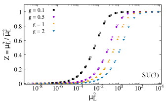
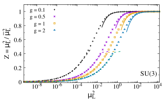
Figure 1: (Left) Lattice spacing dependence of the renormalization factor $Z$ from a non-perturbative calculation for SU(3) for (filled points) $L=11.5$ fm and $\mu=3$ GeV and (open points) $L\approx 1.77$ fm and $\mu=0.35$ GeV showing scaling invariance. (Right) Comparison of analytical results with the non-perturbative calculation. Solid lines are the result from Eq. (37), valid for $Z\sim 1$; dashed lines represent the solution of Eq. (39), valid for $Z\sim 0$, with the leading and next-to-leading order terms in lattice spacing. For asymptotically small values of $\mu_{L}$ the dashed curves reduce to Eq. (40).

Next we consider the lattice spacing dependence of the renormalization factor $Z$. Following Krasnitz:1998ns , we write $\mu_{L}=\mu\,a$. The filled points in left panel of Fig. 1 were obtained for a lattice of size $L=11.5$ fm, which corresponds to the radius $R=6.5$ fm of a gold nucleus by the relation $L^{2}=\pi R^{2}$, and using $\mu=3$ GeV in the MV model. As $\mu$ is kept fixed, the $\mu_{L}$ dependence is obtained by solving Eq. (9) for decreasing values of the lattice spacing, which are obtained by successively increasing the number of sites of the lattice by a factor of two while keeping its volume fixed ($L^{2}=N_{s}^{2}\,a^{2}=$ constant) at each step. For instance, the rightmost point is the result for a lattice with $N_{s}=2$, the next one is the result for a lattice with $N_{s}=2^{2}$ and so on, with the last point shown in the figure corresponding to a lattice with $N_{s}=2^{22}$. As the infinite nucleus approximation throws away any detailed information about the geometry of all physical systems, one should expect exact scale invariance. This means that the only difference between a hadron and a heavy nucleus should be the size of the lattice in physical units, so both are related by a simple scaling factor. Consequently, once the coupling $g$ is fixed, results for different systems should all fall under the same curve, with all physics being controlled by the dimensionless quantity $\mu_{L}$. To show that this is the case, the left panel of Fig. 1 also includes the results (open symbols) for a system with $L=1\,\mathrm{fm}\,\sqrt{\pi}\approx 1.77$ fm, with $\mu=0.35$ GeV (which loosely corresponds to a proton). One clearly sees that the results for both systems fall under the same curve, showing the scaling invariance, as expected. Therefore, it is only needed to specify the details of a given system (here completely determined by the lattice size in physical units and color charge $\mu$) when discussing results at fixed lattice size.

In the right panel of Fig. 1, we compare the resulting lattice spacing dependence of the renormalization factor $Z(a)$ from the asymptotic cases considered above with the result from a full non-perturbative calculation for different couplings. We see that $Z\rightarrow 0$ as $a\rightarrow 0$ for all values of the coupling in the full non-perturbative calculation, indicating that Eq. (3) “flows” towards a theory dominated by large non-Gaussian fluctuations. In this renormalization scheme, even though $\bar{\mu}(a)$ has been determined by requiring the matching of the two-point function of color charges in the non-Gaussian theory and the MV model for each lattice size, the matching is achieved by decreasing the renormalization factor, that is, by moving further away from the MV model regardless of the system size. On purely theoretical grounds, nothing is prohibiting such weight functions to exist, however, such a scenario seems unlikely to be realized.

Fig. 2 shows the lattice spacing dependence of the ratio of the correlator of four-color charges in the non-Gaussian ensemble to the Gaussian ensemble for different values of the coupling. As $\bar{\mu}\neq\mu$, results from the Gaussian and non-Gaussian ensembles would fall in different bins in the horizontal axis, and a comparison between them would only be possible after extrapolating the results to the continuum limit. This is circumvented by using the correlator of two-color charges to form dimensionless quantities: $a^{4}\langle\rho^{2}\rangle=a^{2}\mu^{2}=\mu_{L}^{2}$. This is equivalent to assuming the average color charge from the MV model as a momentum scale in the horizontal axis. Our results show that i) for $\mu_{L}\gg g$ there is no deviation from the Gaussian theory, and the ratio is one; ii) for $\mu_{L}\lesssim g$ there is a smooth transition from a Gaussian dominated distribution (where the perturbative calculation from Dumitru:2011zz applies) to a distribution which is more and more dominated by the quartic term. The resulting effect is the gradual reduction of the higher-order correlator of color charges, in accordance with increasing deviations from the MV model presented Fig. 1; iii) such transition shows a hierarchy with the coupling constant, the agreement with the perturbative result breaks first for larger values of $g$ at fixed $\mu_{L}$; iv) once the distribution of color charges is dominated by the non-Gaussian term ($Z\to 0$), the ratio converges to the continuum limit value shown in Eq. (34a) for SU(2) and Eq. (34b) for SU(3) for all values of the coupling and $\mu_{L}$.

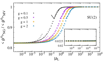
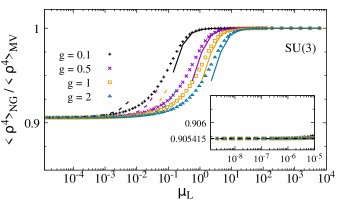
Figure 2: The ratio of the correlator of four-color charges in the non-Gaussian to the Gaussian ensemble as a function of $\mu_{L}$ for (left) SU(2) and (right) SU(3) color symmetry group. The solid lines represent the perturbative results for $Z\sim 1$, Eq. (38), while the dashed ones are the result of solving Eq. (39) with all terms presented. For asymptotically small values $\mu_{L}$, which corresponds to the $Z\to 0$ limit, the dashed curves reduce to the values in Eq. (34a) for SU(2) and Eq. (34b) for SU(3), respectively. The inset plots extend our results up to $\mu_{L}\sim 10^{-8}$, showing that indeed the results converged to the continuum limit.

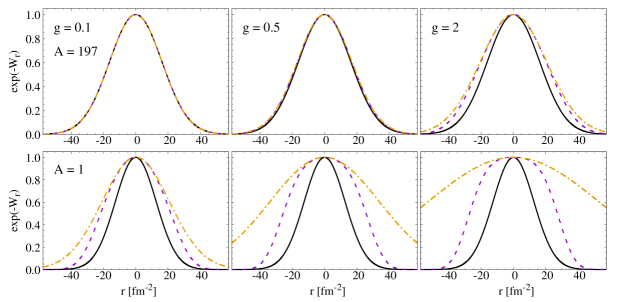
Figure 3: Weight function from a Gaussian (solid line) and non-Gaussian (dashed line) ensembles for a system with (top panels) $L=11.5$ fm and $\mu=3.0$ GeV and (bottom panels) $L\approx 1.77$ fm and $\mu=0.35$ GeV and different values of the coupling in SU(3) in a lattice with $N_{s}=128$. The dashed-dotted line is a Gaussian distribution with the standard deviation equal to the renormalized average color charge $\bar{\mu}$.

Let us look at how far away the non-Gaussian distribution is from a Gaussian distribution. Fig. 3 shows the weight function from the MV model (full line) and the respective non-Gaussian ensemble (dashed line) for (top panels) a Gold-like system ($L=11.5$ fm) with $\mu=3$ GeV and (bottom panels) a proton-like system ($L=1\,\mathrm{fm}\,\sqrt{\pi}\approx 1.77$ fm) with $\mu=0.35$ GeV for different values of $g$ for SU(3) as a function of $r^{2}\equiv\sum_{a=1}^{N_{c}^{2}-1}(\rho^{a}_{x})^{2}$. These weight functions were obtained in a lattice with $N_{s}=128$, corresponding to $\mu_{L}\sim 1.37$ ($\mu_{L}\sim 0.025$) for a Gold-like (proton-like) system. The dashed-dotted line represents a Gaussian distribution with the standard deviation $\bar{\mu}_{L}$. We note that the distributions for SU(2) have the same features. The color charge distribution in the large system with small $g$ is described well as Gaussian. For $g=2$, the quartic term starts to dominate, and the resulting distribution gradually deviates from a Gaussian distribution. On the other hand, small systems already present strong deviations from the perturbative regime for all values of $g$ considered.

IV.2 Renormalization equation in SU($N_{c}$) for the second renormalization scheme

In this section, we consider the second renormalization scheme, in which $\kappa_{4}$ is kept fixed to a given constant value. This renormalization presents an important difference from the previous one: $\kappa_{4}$ and $Z$ are treated as independent parameters.

In the regime where the quartic term is a small perturbation, $Z$ is determined by $\kappa_{4}$ through Eq. (18):

$$Z(a,\kappa_{4})=1-\frac{12\,(N_{c}^{2}+1)\,\bar{\mu}^{4}}{\kappa_{4}\,a^{2}}\,.$$ (41)

As we keep the calculation at order ${\mathcal{O}}[1/\kappa_{4}]$, we replace $\bar{\mu}^{4}/\kappa_{4}$ by $\mu^{4}/\kappa_{4}$, and $Z$ is given by:

$$Z(a,\kappa_{4})=1-\frac{12\,(N_{c}^{2}+1)\,\mu^{4}}{\kappa_{4}\,a^{2}}\,.$$ (42)

On the other hand, in the limit of large non-Gaussian fluctuations, solving Eq. (25) for $Z$ yields:

$$Z(a,\kappa_{4})=\frac{2\,\mu^{2}\,\Gamma\left(\frac{1}{4}\left(N_{c}^{2}-1\right)\right)\left[\sqrt{3\,\kappa_{4}}\,a\,\,\Gamma\left(\frac{1}{4}\left(N_{c}^{2}+1\right)\right)-12\,\mu^{2}\,\Gamma\left(\frac{1}{4}\left(N_{c}^{2}+3\right)\right)\right]}{\left[\Gamma\left(\frac{1}{4}\left(N_{c}^{2}-1\right)\right)\Gamma\left(\frac{1}{4}\left(N_{c}^{2}+3\right)\right)-\Gamma\left(\frac{1}{4}\left(N_{c}^{2}+1\right)\right)^{2}\right]\,a^{2}\,\kappa_{4}}\,.$$ (43)

Eq. (43) fixes $Z(a,\kappa_{4})$ so that the non-Gaussian action reproduces the two-point function of color charges from the Gaussian theory. We note that $Z(a,\kappa_{4})$ will change the sign at some point in this second renormalization scheme. The sign of $Z(a,\kappa_{4})$ is determined by the factor $\sqrt{3\,\kappa_{4}}\,a\,\,\Gamma\left(\frac{1}{4}\left(N_{c}^{2}+1\right)\right)-12\,\mu^{2}\,\Gamma\left(\frac{1}{4}\left(N_{c}^{2}+3\right)\right)$. In particular, $Z$ will become zero when

$$a=\frac{4\,\sqrt{3}\,\Gamma\left(\frac{1}{4}\left(N_{c}^{2}+3\right)\right)}{\Gamma\left(\frac{1}{4}\left(N_{c}^{2}+1\right)\right)}\frac{\mu^{2}}{\sqrt{\kappa_{4}}}\,,$$ (44)

and the renormalization factor becomes negative for the lattice spacing smaller than the value given by Eq. (44). In fact, as $a\rightarrow 0$, Eq. (43) becomes

$$Z(a,\kappa_{4})=-\frac{24\,\mu^{4}}{\left(1-\frac{\Gamma\left(\frac{1}{4}\left(N_{c}^{2}+1\right)\right)^{2}}{\Gamma\left(\frac{1}{4}\left(N_{c}^{2}-1\right)\right)\Gamma\left(\frac{1}{4}\left(N_{c}^{2}+3\right)\right)}\right)\,a^{2}\kappa_{4}}\,=\,-\frac{\mu^{4}}{a^{2}\,\kappa_{4}}\times\begin{cases}88.718,&\text{for }\mathrm{SU(2)}\\ 206.138,&\text{for }\mathrm{SU(3)}\,,\end{cases}$$ (45)

thus, one cannot take the continuum limit in this renormalization scheme.

Fig. 4 shows the lattice spacing dependence of the renormalization factor in this renormalization scheme. The points represent the result from a numerical calculation in SU(3) for a proton-like system ($\mu=0.35$ GeV and $L\approx 1.77$ fm) for $\kappa_{4}^{1/6}=10$ GeV and $\kappa_{4}^{1/6}=100$ GeV. We expect similar behavior for other parameters. The solid curve in each panel represents the result from Eq. (42) valid for $Z\sim 1$. The dashed curve is the result from Eq. (43) valid for $Z\sim 0$. Eq. (42) is in accordance with the non-perturbative calculation for $Z\sim 1$, while Eq. (43) is able to match the non-perturbative calculation for $Z\to 0$.

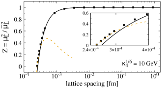
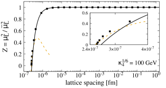
Figure 4: Renormalization factor $Z(a,\kappa_{4})$ in the second renormalization scheme in SU(3) from full non-perturbative calculation (points) for (left) $\kappa_{4}^{1/6}=10$ GeV and (right) $\kappa_{4}^{1/6}=100$ GeV. The solid curve is the result from Eq. (42). The dashed curve is the result from Eq. (43).

As in the previous renormalization scheme, the renormalization factor $Z(a,\kappa_{4})$ is close to one at large $a$, indicating no deviation from the Gaussian theory. However, its dependence with the lattice spacing changes quite drastically as $a\to 0$, with $Z(a,\kappa_{4})$ now presenting a sharper decrease. Eq. (43) matches the full numerical calculation in the $Z\rightarrow 0$ limit. We verified via a numerical calculation that once $Z=0$, there is no solution for the renormalization equation as we only have the quartic term, whose coupling $\kappa_{4}$ is kept fixed in this renormalization scheme.

IV.3 Multi-point correlators of color charges and the renormalization equation in SU($N_{c}$) for the third renormalization scheme

In the third renormalization scheme, the renormalization factor $Z$ is kept fixed. Thus, this renormalization scheme provides a way to control deviations from the MV model even in the limit of large non-Gaussian fluctuations.

In the regime of small non-Gaussian fluctuations, from Eq. (42), $\kappa_{4}$ is given by

$$\kappa_{4}(a,Z)=12\frac{\mu^{4}}{1-Z}\frac{(N_{c}^{2}+1)}{a^{2}}\,.$$ (46)

The $Z\rightarrow 1$ limit leads to $\kappa_{4}\rightarrow\infty$, thus recovering the MV model. The $a\rightarrow 0$ limit with $Z<1$ also leads to $\kappa_{4}\rightarrow\infty$. However, this does not mean it reduces exactly to the MV model as far as $Z$ is different from one.

The four-point function of color charges is obtained by substituting $\kappa_{4}$ from Eq. (46) into Eq. (24),

$$\frac{\langle\rho^{a}_{x}\rho^{a}_{x}\rho^{c}_{x}\rho^{c}_{x}\rangle_{\text{NG}}}{\langle\rho^{a}_{x}\rho^{a}_{x}\rho^{c}_{x}\rho^{c}_{x}\rangle_{\text{MV}}}=1-\frac{2\,(1-Z)}{(N_{c}^{2}+1)}\,.$$ (47)

We see that the ratio of four-point functions in the non-Gaussian to the Gaussian theory is independent of the lattice spacing. This is a exclusive feature of this renormalization scheme, given that $Z$ changes with the lattice spacing in the other two renormalization schemes.

In the limit of large non-Gaussian fluctuations, the renormalization equation (Eq. (25)) is a quadratic equation for $\kappa_{4}$, and has two solutions:

$$\kappa_{4}(a,Z)\equiv\frac{\kappa_{4}(Z)}{a^{2}}=\frac{6\,\mu^{4}\,\left[\alpha(Z)\pm\beta(Z)\right]}{a^{2}\,Z^{2}\,\Gamma_{\frac{1}{4},1}^{2}\,(\Gamma_{\frac{1}{4},1}^{2}-\Gamma_{\frac{1}{4},-1}\,\Gamma_{\frac{1}{4},3})^{2}}$$ (48)

where $\Gamma_{k,m}\equiv\Gamma\left(k\,(N_{c}^{2}+m)\right)$ and

$$\alpha(Z) = 2^{3-N_{c}^{2}}\,\pi\,\Gamma_{\frac{1}{2},-1}^{2}\left(\,\Gamma_{\frac{1}{4},1}^{2}\left(\left(N_{c}^{2}-1\right)Z+1\right)-4\,Z\,\Gamma_{\frac{1}{4},3}^{2}\,\right)$$ (49)

$$\beta(Z) = \Gamma_{\frac{1}{4},-1}^{3/2}\,\Gamma_{\frac{1}{4},1}^{3}\,\left[8\,Z\,\Gamma_{\frac{1}{4},3}\,\Gamma_{\frac{1}{4},1}^{2}+\Gamma_{\frac{1}{4},-1}\,\left(\Gamma_{\frac{1}{4},1}^{2}-8\,Z\,\Gamma_{\frac{1}{4},3}^{2}\right)\right]^{1/2}\,.$$ (50)

We verified that the two solutions above lead to different results in the $Z\to 0$ limit. Setting $N_{c}=3$ in order to have a compact expression and further expanding the solution above proportional to $\alpha(Z)-\beta(Z)$ around $Z=0$, then dividing it by the leading order expression for $\kappa_{4}$ (Eq. (27)) gives

$$\frac{\kappa_{4}^{\text{LO+NLO}}}{\kappa_{4}^{\text{LO}}}=1+1.05415\,Z+1.38903\,Z^{2}\,.$$ (51)

Repeating the same procedure with the solution proportional to $\alpha(Z)+\beta(Z)$ yields terms proportional to $1/Z^{2}$ and $1/Z$, thus not recovering the leading order solution. Because of this, we discard such a solution.

Let us turn now to the computation of the four-point function of color charges. Using the solution for $\kappa_{4}$ proportional to $\alpha(Z)-\beta(Z)$ in Eq. (26) provides an expression for the correlator of four-color charges at the delta functions for an arbitrary value of $N_{c}$. The ratio of the correlator of color charges in the non-Gaussian to the Gaussian theory at leading order in the renormalization factor can be written as:

$$\frac{\langle\rho^{a}_{x}\rho^{a}_{x}\rho^{c}_{x}\rho^{c}_{x}\rangle_{\text{NG}}}{\langle\rho^{a}_{x}\rho^{a}_{x}\rho^{c}_{x}\rho^{c}_{x}\rangle_{\text{MV}}}= \frac{(-d_{0}+D)^{2}}{4(N_{c}^{2}+1)\,d_{1}^{2}\,Z^{2}}\left(1+\frac{d_{0}}{d_{1}}(d_{0}-D)\right)\,,\qquad D=\sqrt{d_{0}^{2}+2d_{1}\,Z}$$ (52)

where

$$d_{0} \equiv \frac{1}{4}\frac{\Gamma((N_{c}^{2}+1)/4)}{\Gamma((N_{c}^{2}+3)/4)}\,,$$ (53)

$$d_{1} \equiv d_{0}^{2}\,(N_{c}^{2}-1)-\frac{1}{4}\,.$$ (54)

As in Eq. (47), valid in the limit of small non-Gaussian fluctuations, this ratio remains independent of the lattice spacing and is constant for fixed $Z$ in the limit of large non-Gaussian fluctuations.

The left panel of Fig. 5 shows the lattice spacing dependence of the ratio of the correlators of four-color charges at the delta functions in the non-Gaussian and the Gaussian theories for different values of $Z$. Smaller values of $Z$ lead to a larger deviation from the MV model. The curves at $Z=0.9999\sim 1$ and $Z=0.01$ are given by Eq. (47) and Eq. (52) respectively, which nicely reproduce the results of the non-perturbative calculations.

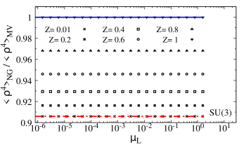
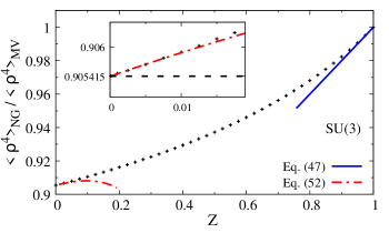
Figure 5: (Left) Lattice spacing dependence of the ratio of four-point function of color charges in the non-Gaussian to the Gaussian theory for different values of the renormalization factor $Z$ for $L=1.77$ fm and $\mu=0.35$ GeV. (Right) Dependence of the same ratio with $Z$. The inset plot shows that $Z\rightarrow 0$ recovers the leading order result (Eq. (34b)) shown as a dashed line.

The right panel in Fig. 5 shows the $Z$ dependence of the same ratio with points representing the results from the non-perturbative calculation together with the perturbative results from Eq. (47) and Eq. (52). We see that for both small and large non-Gaussian fluctuations, the analytical results are in good agreement with the non-perturbative ones. It is also shown that the ratio converges to the result given by Eq. (34b) in the $Z\to 0$ limit.

V Conclusions

In this work, we studied the non-perturbative effects of the first (even C-parity) non-Gaussian correction to the Gaussian theory of the CGC in SU(2) and SU(3) color symmetry groups. Deviations from the MV model were quantified via the renormalization factor, $Z$. The couplings in the non-Gaussian small-$x$ action need to be renormalized in order to reproduce the two-point function of color charges in the Gaussian theory. We considered three different renormalization schemes to determine the couplings of the non-Gaussian action. New analytical expressions were presented in the regime of large non-Gaussian fluctuations in each renormalization scheme and these were compared to numerical results where the renormalization equation, Eq. (12), was solved numerically. Our results pointed out that the first two renormalization schemes always lead to a theory dominated by non-Gaussian fluctuations independent of the system size. This means that even larger systems end up being strongly affected by non-Gaussian corrections. Such a scenario is unlikely to happen, as one expects the validity of the MV model for larger systems. The third renormalization scheme, where $Z$ is fixed, on the other hand, allows one to control the deviations from the MV model. The strength of the non-Gaussian correction to the MV model in physical observables is still an open question and deserves further investigation. The next step is to determine the values of $Z$ by considering experimental data to see to what extent a system deviates from the MV model.

The calculations shown here represent the first practical step towards making non-Gaussian initial conditions to the JIMWLK evolution equations. In addition, we showed that the initial distribution of color charges moves away from a Gaussian once deviations from the MV model are considered. The quartic term should affect the multiplicity distribution, especially in small collision systems, where non-Gaussian corrections are usually expected. That would change the fluctuations of the energy (or gluon) density in the initial condition for hydrodynamic simulations. In particular, fluctuations of the initial energy density are important to determine spatial eccentricities Dumitru:2012yr , which can be related to flow harmonics and angular correlations in hydrodynamic simulations Ollitrault:1992bk ; Poskanzer:1998yz ; Alver:2010gr ; Qin:2010pf ; Teaney:2010vd ; Gardim:2011xv ; Qiu:2011iv ; Bozek:2012gr . Such changes also apply to early time fluctuations of axial charge density in the glasma phase, which are given in terms of the divergence of the Chern-Simons current Lappi:2017skr ; Guerrero-Rodriguez:2019ids .

Furthermore, as shown in Dumitru:2011ax , the inclusion of a quartic term in the weight function generates a correction to the correlator of two Wilson lines, $\langle V(x)V^{\dagger}(y)\rangle$, where $V(x)$ denotes a Wilson line. For this reason, such initial conditions may be used to study whether there exist differences between the JIMWLK evolution with and without assuming the Gaussian approximation, where all higher $n$-point function of Wilson lines can be related to $\langle V(x)V^{\dagger}(y)\rangle$ Iancu:2011nj .

The calculations in this paper can be extended to study the non-Gaussian effects on the two-particle correlation function, $C_{2}(p,q)$ in the double inclusive gluon production Lappi:2009xa and the dipole operator, $D(r)\propto\langle V(x)V^{\dagger}(y)\rangle$, complementing the results in the dilute regime from Dumitru:2011ax . In particular, it has been shown Dumitru:2011zz that at the perturbative level the quartic term generates an additional contribution of the same order in $N_{c}$ to $C_{2}(p,q)$ on top of the contribution from the Gaussian part of the action. Moreover, the non-Gaussian correction becomes of the same order in the mass number and is enhanced by a factor of $N_{c}^{2}-1$ compared to the Gaussian contribution if one considers the saturation scale as a cutoff for integrals over transverse momentum figuring in this quantity. A non-perturbative calculation is needed to access how the effects of additional contributions from a non-Gaussian statistics change the result from the MV model to all orders of $1/\kappa_{4}$ in this case. Works in these directions are ongoing.

- (1) E. Iancu and R. Venugopalan, In *Hwa, R.C. (ed.) et al.: Quark gluon plasma* 249-3363, [hep-ph/0303204]; F. Gelis, E. Iancu, J. Jalilian-Marian and R. Venugopalan, Ann. Rev. Nucl. Part. Sci. 60, 463 (2010).
- (2) Y. V. Kovchegov, Phys. Rev. D 60, 034008 (1999); H. Weigert, Prog. Part. Nucl. Phys. 55, 461 (2005); J. P. Blaizot, F. Gelis and R. Venugopalan, Nucl. Phys. A 743, 13 (2004); J. P. Blaizot, F. Gelis and R. Venugopalan, Nucl. Phys. A 743, 57 (2004); H. Weigert, Prog. Part. Nucl. Phys. 55, 461 (2005).
- (3) J. Jalilian-Marian, A. Kovner, L. D. McLerran and H. Weigert, Phys. Rev. D 55, 5414 (1997).
- (4) J. Jalilian-Marian, A. Kovner, A. Leonidov and H. Weigert, Nucl. Phys. B 504, 415 (1997).
- (5) J. Jalilian-Marian, A. Kovner, A. Leonidov and H. Weigert, Phys. Rev. D 59, 014014 (1998).
- (6) J. Jalilian-Marian, A. Kovner and H. Weigert, Phys. Rev. D 59, 014015 (1998).
- (7) J. Jalilian-Marian, A. Kovner, A. Leonidov and H. Weigert, Phys. Rev. D 59, 034007 (1999); Erratum: [Phys. Rev. D 59, 099903 (1999)].
- (8) A. Kovner and J. G. Milhano, Phys. Rev. D 61, 014012 (2000).
- (9) A. Kovner, J. G. Milhano and H. Weigert, Phys. Rev. D 62, 114005 (2000).
- (10) E. Iancu, A. Leonidov and L. D. McLerran, Nucl. Phys. A 692, 583 (2001).
- (11) E. Iancu, A. Leonidov and L. D. McLerran, Phys. Lett. B 510, 133 (2001).
- (12) E. Ferreiro, E. Iancu, A. Leonidov and L. McLerran, Nucl. Phys. A 703, 489 (2002).
- (13) L. D. McLerran and R. Venugopalan, Phys. Rev. D 49, 2233 (1994), Phys. Rev. D 49, 3352 (1994), Phys. Rev. D 50, 2225 (1994).
- (14) C. S. Lam and G. Mahlon, Phys. Rev. D 64, 016004 (2001).
- (15) A. Dumitru, J. Jalilian-Marian, T. Lappi, B. Schenke and R. Venugopalan, Phys. Lett. B 706, 219 (2011).
- (16) C. Marquet, Nucl. Phys. A 796, 41 (2007).
- (17) F. Dominguez, C. Marquet, B. W. Xiao and F. Yuan, Phys. Rev. D 83, 105005 (2011).
- (18) T. Lappi, B. Schenke, S. Schlichting and R. Venugopalan, JHEP 1601, 061 (2016).
- (19) S. Jeon and R. Venugopalan, Phys. Rev. D 70, 105012 (2004); Phys. Rev. D 71, 125003 (2005).
- (20) A. Dumitru, J. Jalilian-Marian and E. Petreska, Phys. Rev. D 84, 014018 (2011).
- (21) A. Dumitru and E. Petreska, Nucl. Phys. A 879, 59 (2012).
- (22) A. Dumitru and E. Petreska, arXiv:1209.4105 [hep-ph].
- (23) A. Kovner and M. Lublinsky, Phys. Rev. D 83, 034017 (2011).
- (24) K. J. Golec-Biernat and M. Wusthoff, Phys. Rev. D 59, 014017 (1998).
- (25) A. Dumitru and J. Jalilian-Marian, Phys. Rev. D 81, 094015 (2010).
- (26) A. Dumitru, private communication.
- (27) A. Krasnitz and R. Venugopalan, Nucl. Phys. B 557, 237 (1999).
- (28) A. Dumitru and Y. Nara, Phys. Rev. C 85, 034907 (2012).
- (29) J. Y. Ollitrault, Phys. Rev. D 46, 229 (1992).
- (30) A. M. Poskanzer and S. A. Voloshin, Phys. Rev. C 58, 1671 (1998).
- (31) B. Alver and G. Roland, Phys. Rev. C 81, 054905 (2010) Erratum: [Phys. Rev. C 82, 039903 (2010)].
- (32) G. Y. Qin, H. Petersen, S. A. Bass and B. Muller, Phys. Rev. C 82, 064903 (2010).
- (33) D. Teaney and L. Yan, Phys. Rev. C 83, 064904 (2011).
- (34) F. G. Gardim, F. Grassi, M. Luzum and J. Y. Ollitrault, Phys. Rev. C 85, 024908 (2012).
- (35) Z. Qiu and U. W. Heinz, Phys. Rev. C 84, 024911 (2011).
- (36) P. Bozek and W. Broniowski, Phys. Lett. B 718, 1557 (2013).
- (37) T. Lappi and S. Schlichting, Phys. Rev. D 97, no. 3, 034034 (2018).
- (38) P. Guerrero-Rodríguez, JHEP 1908, 026 (2019).
- (39) E. Iancu and D. N. Triantafyllopoulos, JHEP 1204, 025 (2012).
- (40) T. Lappi, S. Srednyak and R. Venugopalan, JHEP 1001, 066 (2010).