Resilient Consensus via Weight Learning and Its Application in Fault-Tolerant Clock Synchronization

Abstract

This paper addresses the distributed consensus problem in the presence of faulty nodes. A novel weight learning algorithm is introduced such that neither network connectivity nor a sequence of history records is required to achieve resilient consensus. The critical idea is to dynamically update the interaction weights among neighbors learnt from their credibility measurement. Basically, we define a reward function that is inversely proportional to the distance to its neighbor, and then adjust the credibility based on the reward derived at the present step and the previous credibility. In such a way, the interaction weights are updated at every step, which integrates the historic information and degrades the influences from faulty nodes. Both fixed and stochastic topologies are considered in this paper. Furthermore, we apply this novel approach in clock synchronization problem. By updating the logical clock skew and offset via the corresponding weight learning algorithms, respectively, the logical clock synchronization is eventually achieved regardless of faulty nodes. Simulations are provided to illustrate the effectiveness of the strategy.

1 Introduction

Multi-agent consensus is a fundamental problem in distributed systems, and has been studied for decades in the fields of computer science, control, communication and many others. The objective is to achieve global agreement with local collaborative interactions. In practice, faulty agents with non-cooperative behaviors are inevitable to interfere system coordination, such as Internet ghostwriters to influence public opinions, enemy aircrafts to disturb unmanned aerial vehicle formation control, malfunctioning clocks to break clock synchronization, and so on [1]. How to effectively identify all the faulty nodes and eliminate their negative effects so as to achieve resilient consensus is a challenging problem.

A typical method is to remove the extreme neighbor nodes at state updating. This method is available only if the network connectivity is not less than $2F+1$, where $F$ is the maximal number of faulty nodes [2, 3]. In [4], the authors presented a Mean-Subsequence-Reduced (MSR) algorithm that combines ideas of distributed computing and control consensus protocols to solve the asymptotic consensus under the $F$-total malicious model in complete networks. This MSR algorithm was further generalized to the Weighted-Mean-Subsequence-Reduced (W-MSR) algorithm to solve both malicious and Byzantine threat models [5]. Following the idea, an asynchronous delayed network case was considered [6]. In [7], the authors provided tight conditions for resilient consensus using the MSR algorithm. In addition, the authors of [8] proposed a novel topological property where network robustness replaces the network connectivity metrics. This kind of methods by removing the extreme neighbor nodes are constrained to the network connectivity or network robustness and hardly realized in practice.

Another way to solve the consensus problem with faulty nodes is to evaluate the trustworthiness on each neighbor node. The trustworthiness is typically determined by a weight measuring the influence of the neighbor nodes. In [9], the authors presented an algorithm named RoboTrust, to calculate trustworthiness of agents using observations and statistical inferences from various historical perspectives, and thus all the agents finally converge to the value agreed by the most trustworthy agents. The trustworthiness established by local evidence in [9] was extended to the second-hand evidence in [10]. The trustworthiness based consensus strategy with faulty nodes avoids the network connectivity or network robustness, yet requires to store and analyze a mass of historical information.

To overcome the disadvantage of requiring network connectivity or network robustness, or storage and analysis of historical information, this paper presents a Weight Learning Algorithm (WLA) borrowing the idea from Reinforcement Learning (RL) [11, 12]. In a multi-agent consensus problem, adjacent weights between two neighbor nodes indicate the strength of influence. Therefore, the goal is to isolate the faulty nodes by reducing the adjacent weights to zero in a local consensus protocol. To achieve it, we first construct a reward function by the relative distance of neighbor nodes. Next, each credibility is updated by its previous value and the reward at the present step. Finally, all the adjacent weights are determined by the credibility via normalization. In this way, the adjacent weights from faulty nodes become smaller compared to the ones from normal nodes, and tend to zero.

We consider three different classes of nodes in this paper, represented by normal nodes, persistent faulty nodes [13, 8], and intermittent faulty nodes. Persistent faulty nodes may take arbitrary uncertain states at each time due to faults or external attacks. Intermittent faulty nodes, which is a mixed behavior of normal nodes and that of persistent faulty nodes with a certain probability, inject hostile influence to the network intermittently by not being easily detected. Furthermore, we apply this novel approach in a clock synchronization problem.

Clock synchronization is a common and fundamental problem in wireless sensor networks (WSNs), for various applications such as scheduling, information fusion, and so on. The substantial results in analyzing this problem include Reference Broadcast Synchronization [14], Timing-sync Protocol for Sensor Networks [15], Lightweight Time Synchronization, Flooding Time Synchronization Protocol [16], and Consensus Based Synchronization Protocol [17, 18, 19, 20, 13]. Among these, the consensus-based approach is popular in recent years due to its scalability, robustness, distributed manner, and simple implementability.

The consensus-based protocols can be classified into two categories, i.e., Average Time Synchronization (ATS) [17] and Maximum Time Synchronization (MTS) [18]. In ATS, each node utilizes the average value of neighbor nodes and its own to achieve consensus, and in MTS, this value becomes the maximum of the neighbors and the node itself. In [19], the authors present the second-order consensus strategy to solve the clock synchronization problem under measurement noises and time-varying clock drifts. [20] proposes a modified MTS algorithm to speed up convergence under bounded noise. [13] borrows the idea of MSR algorithm to remove the outliers in the clock data received from the neighbors to deal with the unreliable channels in WSNs.

In this paper, we consider the clock synchronization problem with bounded system noise. As some nodes in the network may be hacked and transmit arbitrary signals (occasionally) by not following the given protocol, we construct logical clock skew and offset, and update their values via WLA. As a result, the faulty nodes are gradually isolated and all the normal nodes achieve resilient logical clock synchronization.

The contributions of this paper are as follows:

1. Most references assume various network conditions, such as $F$-total fault model (up to $F$ faulty nodes), $F$-local fault model (up to $F$ faulty incoming neighbors for each normal node), or network connectivity (no less than $2F+1$). The proposed algorithm only requires a rooted communication topology among normal nodes.

2. Some references without assuming the aforementioned network conditions require a mass of historical information to analyze, that is hard to realize in large scale networks. The proposed algorithm is simple and efficient by integrating all the historical information into one variable.

3. Two different misbehaved models are considered for both fixed and stochastic topologies in this paper.

4. The proposed approach is applied in a clock synchronization problem with hacked or malfunctioning nodes and system noise, and hence achieves resilient logical clock synchronization for all normal nodes.

The rest of this paper is organized as follows. Section 2 introduces necessary preliminaries and system models. The detailed WLAs for both fixed communication topology and stochastic communication topology are given in Section 3. Section 4 discusses the clock synchronization problem and the corresponding solution by our approach. Numerical simulations and conclusions are presented in Sections 5 and 6, respectively.

2 Preliminaries and Problem Formulation

In this paper, we consider the consensus problem in a point-to-point message-passing network, which is thus modeled as a directed graph (digraph). Given a digraph $G=(V,E,A)$ where $V=\{1,2,\cdots,n\}$ is the node set, $E\subseteq V\times V$ is the edge set, and $A=\{[a_{ij}]\geq 0\}$ represents the weighted adjacency matrix. An edge $(j,i)\in E$ exists if and only if there is information flow from node $j$ to node $i$, i.e., $a_{ij}>0$. It is assumed $a_{ii}=0$ with no self-loop. The neighbor set of node $i$ is presented by $N_{i}=\{j\;|\;(j,i)\in E\}$. A path from node $j$ to $i$ is a sequence of distinct nodes $i_{0},i_{1},\cdots,i_{m}$, where $i_{0}=j$ and $i_{m}=i$ with $(i_{l},i_{l+1})\in E,0\leq l\leq m-1$. We say a digraph rooted if there exists a node $i\in V$, called root, such that there is a path from node $i$ to any other node. We use the terms node and agent interchangeably. The notations $a_{ij}(k)$ and $N_{i}(k)$ are used when they vary with time $k$.

We consider $n$ agents with a discrete-time system model

$$x_{i}(k+1)=x_{i}(k)+u_{i}(k),\;i\in V$$ (1)

where $x_{i}(k)\in\mathbb{R}$ and $u_{i}(k)\in\mathbb{R}$ represent the state and control input of node $i$, respectively. The initial state of the $n$ nodes, i.e., $\mathbf{x}(0)=[x_{1}(0),\cdots,x_{n}(0)]^{T}$, is arbitrarily specified.

In a traditional consensus problem, all nodes are assumed equally trustworthy to cooperate with each other to achieve state consensus [21, 22], through proper design of $u_{i}(k)$. In this paper, we consider three different classes of nodes, represented by the set of normal nodes $V^{\rm n}$, the set of persistent faulty nodes $V^{\rm p}$, and the set of intermittent faulty nodes $V^{\rm i}$, with

$$V=V^{\rm n}\cup V^{\rm p}\cup V^{\rm i}.$$

The faulty nodes include passive ones caused by system failure and active adversarial ones that deliberately inject hostile influence to the network. The control actions for the three sets of nodes are described as follows.

1. Normal Node: The following consensus algorithm is executed in a normal node,

   $$u_{i}(k)=\!\!\!\sum_{j\in N_{i}(k)}\!\!a_{ij}(k)(x_{j}(k)-x_{i}(k))+\omega_{i}(k),\;i\in V^{\rm n},$$ (2)

   where $a_{ij}(k)$ is the adjacent weight from node $j$ to node $i$ satisfying $\sum_{j\in N_{i}(k)}a_{ij}(k)<1$, and $\omega_{i}(k)\in\mathbb{R}$ is a bounded noise ($|\omega_{i}(k)|<\omega$) introduced by transmission channel and environment.

2. Persistent Faulty Node (PFN): A PFN conducts its input with a random value at every time as follows

   $$u_{i}(k)={\rm Random},\;i\in V^{\rm p},$$ (3)

   where $\rm Random$ is a random variable that has a specified probability density function $f_{\rm Random}$.

3. Intermittent Faulty Node (IFN): An IFN mixes the behavior of a normal node and that of a PFN with a certain probability, that is,

   $$u_{i}(k)=\left\{\begin{array}[]{ll}\sum\limits_{j\in N_{i}(k)}a_{ij}(k)(x_{j}(k)-x_{i}(k))+\omega_{i}(k),\\ &\mbox{with probability }p\\ {\rm Random},&\mbox{else}\end{array}\right.,$$

   $$i\in V^{\rm i}.$$

   It especially describes the behavior of a node that acts normally most time not to be detected but intermittently disturbs the network using random actions.

Remark 1

It is worth mentioning that the assumption $a_{ij}(k)\in\{0\}\cup[c,1]$ with $c$ a positive constant is widely used in the traditional consensus settings; see, e.g., [23]. That is, the nonzero weights must be sufficiently away from zero with a lower bound. However, in the present setting, this assumption is not applied as a mechanism is designed to deliberately tune the weights associated with faulty nodes, ideally to zero, to mitigate their influence on the desired network behavior.

Remark 2

The general actions of faulty nodes like PFN and/or IFN as most frequently referred is taken into consideration in this paper. The intelligent faulty nodes with antagonistic behaviors that can add clever corruptions to avoid detection by the given updating scheme is not covered in this paper, and would be our future research interest.

With the appearance of faulty nodes (PFN and/or IFN), the whole network does not achieve consensus in general. This paper aims to design a distributed algorithm for updating network weights among nodes such that the faulty nodes can be isolated from the normal nodes with the weights from the former to the latter can be tuned to be close to zero, that is

$$\limsup_{k\rightarrow\infty}\max_{i\in V^{\rm n},j\in V^{\rm p}\cup V^{\rm i}}|a_{ij}(k)|<\epsilon$$ (4)

for a sufficiently small $\epsilon$. As a result, we expect that the sub-network of normal nodes can still achieve consensus in the following sense

$$\limsup_{k\rightarrow\infty}\max_{i,j\in V^{\rm n}}|x_{i}(k)-x_{j}(k)|<\varepsilon$$ (5)

for a sufficiently small $\varepsilon$. Throughout the paper, it is assumed that the sub-network of normal nodes is rooted in a fixed topology (or with probability one in a stochastic topology).

The achievement of (5) for the system (1) in the presence of PFN and/or IFN is called resilient consensus in this paper. So, the main objective is to propose a distributed algorithm for updating network weights to achieve resilient consensus.

3 Weight Learning Algorithms

A distributed algorithm for updating network weights in the aforementioned objective is called a Weight Learning Algorithm (WLA) in this section. The idea used in the WLA architecture is borrowed from RL using the so-called reward. In particular, for each normal node $i$ and its neighbor $j$, we use a three-level learning strategy: an immediate reward $r_{ij}$ describing the performance at the current instant, a credibility $Q_{ij}$ integrating the historical trustworthiness up to present, and an updating rule for the corresponding adjacent weight $a_{ij}$. Thus, we expect to adjust and reduce the adjacent weights from faulty nodes to normal nodes through trial-and-error interactions, and hence mitigate the influence of faulty nodes for the final objective of resilient consensus. In the sequel, we will study two cases: a fixed topology case and a stochastic topology case.

3.1 Fixed Topology Case

We first consider the WLA in a network with a fixed communication topology, abbreviated to WLA-F. In the algorithm, a critical concept is a reward denoted by $r_{ij}(k)$ for all normal nodes $i\in V^{\rm n}$ and with their neighbors $j\in N_{i}$. In particular, a normal node recognizes its own state $x_{i}$ as the true value and evaluates the reward by the relative state of a neighbor node, represented by the following reward function

$$r_{ij}(k)=f(|x_{j}(k)-x_{i}(k)+\omega_{ij}(k)|,k),\;j\in N_{i},\;i\in V^{\rm n}$$

where $\omega_{ij}$ is the unknown noise on the transmission channel from $j$ to $i$ with $|\omega_{ij}|<\omega$. In general, we can select a reward function $f$ as an inverse proportional function, e.g.,

$$f(|x_{j}(k)-x_{i}(k)+\omega_{ij}(k)|,k)=e^{-|x_{j}(k)-x_{i}(k)+\omega_{ij}(k)|\theta(k)}$$

for an appropriately designed parameter $\theta(k)>0$. With such a selection, we restrict the value of the reward function between $0$ and $1$. When the states $x_{i}$ and $x_{j}$ are sufficiently different, the induced reward is close to $0$; when they agree, the reward moves towards $1$.

Based on the reward, we define a credibility $Q_{ij}$ between two nodes,

$$Q_{ij}(k)=Q_{ij}(k-1)r_{ij}(k),\;Q_{ij}(0)=1,\;j\in N_{i},\;i\in V^{\rm n}.$$

It is initialized as $1$ and then recursively updated according to the associated reward $r_{ij}$. A credibility $Q_{ij}$ essentially integrates all the historical information from node $j$ to node $i$. It contains a mechanism that the credibility reduces more significantly if the reward is closer to $0$ due to the major difference between the node states.

Now, it is ready to find a strategy for weight updating and hence a complete WLA-F. By normalization of the credibility of all neighbors for a normal node, we define the weight as

$$a_{ij}(k)=\frac{Q_{ij}(k)}{\sum_{j\in N_{i}}Q_{ij}(k)}(1-\frac{1}{|N_{i}|}),\;j\in N_{i},\;i\in V^{\rm n},$$

where $|N_{i}|$ is the cardinality of $N_{i}$. The design obviously satisfies $\sum_{j\in N_{i}}a_{ij}(k)<1$.

It is noted that $a_{ij}$ is not applicable for PFNs and it does not have to be updated for IFNs. For the complement of notation, the following simple rule is applied

$$a_{ij}(k)=a_{ij}(0),\;j\in N_{i},\;i\in V^{\rm p}\cup V^{\rm i},$$ (6)

with arbitrarily initialized $a_{ij}(0)$ satisfying $\sum_{j\in N_{i}}a_{ij}(0)<1$. Lastly, from the definition of $N_{i}$, it is trivially known that

$$a_{ij}(k)=0,\;j\notin N_{i},\;i\in V.$$ (7)

From the above, the WLA-F is summarized in Algorithm 1 using pseudocode. Also, the closed-loop system takes the following form

$$x_{i}(k+1)= x_{i}(k)+\sum_{j\in N_{i}}a_{ij}(k)(x_{j}(k)-x_{i}(k))$$

$$+\omega_{i}(k),\;i\in V^{\rm n},$$

$$x_{i}(k+1) =x_{i}(k)+{\rm Random},\;i\in V^{\rm p},$$ (8)

and the mixture for $i\in V^{\rm i}$ with the normal node behavior of probability $p$.

1

21:  Initialize $Q_{ij}(0)=1$, $j\in N_{i}$

3

2:  for $k=1;\ k++$ do

43:     for $j=1;\ j<n+1;\ j++$ do

54:        if $j\in N_{i}$ then

65:           $r_{ij}(k)=f(|x_{j}(k)-x_{i}(k)+\omega_{ij}(k)|)$;

7$Q_{ij}(k)=Q_{ij}(k-1)r_{ij}(k)$;

8$a_{ij}(k)=\frac{Q_{ij}(k)}{\sum_{j\in N_{i}}Q_{ij}(k)}(1-\frac{1}{|N_{i}|})$;

6:        else

7:           $a_{ij}(k)=0$;

8:        end if

99:     end for

1010:     $x_{i}(k+1)=x_{i}(k)+\sum\limits_{j\in N_{i}}a_{ij}(k)(x_{j}(k)-x_{i}(k))+\omega_{i}(k)$.

11:  end for

Algorithm 1 WLA-F for a normal node $i\in V^{\rm n}$

3.2 Stochastic Topology Case

In this subsection, we consider the WLA in a stochastic communication topology (WLA-S) where all the communications are stochastic. To tailor the algorithm for this scenario, we need to modify the reward, the credibility, and the weight update rule accordingly.

As the topology is stochastic, a communication edge may occur between a normal node and any other node. Therefore, we must maintain the rewards $r_{ij}(k)$ for a normal node $i\in V^{\rm n}$ and all other nodes $j\in V$. Noting $N_{i}(k)$ is now time-varying, one has

$$r_{ij}(k)=\left\{\begin{array}[]{ll}f(|x_{j}(k)-x_{i}(k)+\omega_{ij}(k)|,k),&j\in N_{i}(k)\\ r_{ij}(k-1),&j\notin N_{i}(k)\end{array}\right.,$$

$$i\in V^{\rm n}$$

with the initial setting

$$r_{ij}(0)=1,\;j\in V,\;i\in V^{\rm n}.$$

In other words, at each time instant, the reward $r_{ij}(k)$ updates in a normal way if node $j$ is a neighbor of node $i$ but keeps the historical value $r_{ij}(k-1)$ otherwise.

With the modified definition of reward, the credibility $Q_{ij}$ is modified accordingly,

$$Q_{ij}(k)=Q_{ij}(k-1)r_{ij}(k),\;i\in V^{\rm n},$$

with the initial values

$$Q_{ij}(0)=1,\;j\in V,\;i\in V^{\rm n}.$$

The weight is thus updated following the rule

$$a_{ij}(k)=\frac{Q_{ij}(k)}{\sum_{j\in N_{i}(k)}Q_{ij}(k)}\gamma,\;j\in N_{i}(k),\;i\in V^{\rm n}$$

where $\gamma\in(0,1)$ is an appropriately selected parameter. It contains a mechanism that the updating of node $i$ relies more on neighbor nodes if the value $\gamma$ is close to $1$, and results probably in a faster convergence rate, which yet may produce unstable performance. It is assured that $\sum_{j\in N_{i}(k)}a_{ij}(k)<1$ always holds. The update rules (6) and (7) are slightly revised as follows

$$a_{ij}(k) =a_{ij}(0),\;j\in N_{i}(k),\;i\in V^{\rm p}\cup V^{\rm i},$$

$$a_{ij}(k) =0,\;j\notin N_{i}(k),\;i\in V.$$

with arbitrarily initialized $a_{ij}(0)$ satisfying $\sum_{j\in V}a_{ij}(0)<1$.

Finally, the WLA-S is summarized in Algorithm 2 using pseudocode. Also, the closed-loop system takes the same form as that in the fixed topology case.

Remark 3

It is worth mentioning that $\gamma=1-\frac{1}{|N_{i}|}$ in fixed topology case. We abandon the usage of $\gamma=1-\frac{1}{|N_{i}(k)|}$ in stochastic topology case to avoid that $|N_{i}(k)|=0$ or $1$.

1

21:  Initialize $Q_{ij}(0)=1$ and $r_{ij}(0)=1$, $j\in V$;

2:  for $k=1;\ k++$ do

33:     for $j=1;\ j<n+1;\ j++$ do

44:        if $j\in N_{i}(k)$ then

55:           $r_{ij}(k)=f(|x_{j}(k)-x_{i}(k)+\omega_{ij}(k)|)$;

6$Q_{ij}(k)=Q_{ij}(k-1)r_{ij}(k)$;

7$a_{ij}(k)=\frac{Q_{ij}(k)}{\sum_{j\in N_{i}(k)}Q_{ij}(k)}\gamma$;

6:        else

87:           $r_{ij}(k)=r_{ij}(k-1)$;

9$Q_{ij}(k)=Q_{ij}(k-1)r_{ij}(k)$;

$a_{ij}(k)=0$;

8:        end if

109:     end for

1110:     $x_{i}(k+1)=x_{i}(k)+\sum\limits_{j\in N_{i}}a_{ij}(k)(x_{j}(k)-x_{i}(k))+\omega_{i}(k)$.

11:  end for

Algorithm 2 WLA-S for a normal node $i\in V^{\rm n}$

4 Application to Clock Synchronization

In this section, we introduce the clock synchronization problem and use it to demonstrate the applicability of the proposed WLA. In particular, it shows that WLA is able to achieve clock synchronization in WSNs when some nodes are faulty or behave abnormally under attack.

4.1 Clock Model

In this paper, we consider a group of $n$ linear clock models [18, 20], each representing a hardware clock whose reading at time $t$ is

$$\tau_{i}^{*}(t)=\alpha_{i}^{*}t+\beta_{i}^{*}.$$ (9)

Here, $\alpha_{i}^{*}$ represents the clock skew that determines the clock speed, and $\beta_{i}^{*}$ denotes the clock offset. Since the clock skews may be slightly different from each other owing to imperfect crystal oscillators, ambient temperature, battery voltage, or oscillator aging [18], we assume that $\alpha_{i}^{*}$ is normalized around 1. It should be noted that the true values of both parameters $\alpha_{i}^{*}$ and $\beta_{i}^{*}$ can not be obtained as the absolute time $t$ is not accessible to the nodes. Therefore, two new parameters $\alpha_{i}(t)$ and $\beta_{i}(t)$ are introduced to produce a logical clock value

$$\tau_{i}(t)=\alpha_{i}(t)\tau_{i}^{*}(t)+\beta_{i}(t)=\alpha_{i}(t)\alpha_{i}^{*}t+\alpha_{i}(t)\beta_{i}^{*}+\beta_{i}(t).$$

We call

$$x^{\prime}_{i}(t)=\alpha_{i}(t)\alpha_{i}^{*},\;x^{\prime\prime}_{i}(t)=\alpha_{i}(t)\beta_{i}^{*}+\beta_{i}(t)$$

the logical clock skew and offset, respectively.

Remark 4

In practice, the clock skew $\alpha_{i}^{*}$ and the clock offset $\beta_{i}^{*}$ vary slowly with time growing. It is expected that the induced errors can be compensated if the proposed synchronization algorithm converges fast enough.

In the system, all the nodes exchange their current information with neighbors periodically with a fixed period $T$. This means that the real period $T_{i}$ for each node $i$ is $T_{i}=T/\alpha_{i}^{*}$. The information exchanged includes the index $i$, original time $\tau_{i}^{*}(t)$, logical time $\tau_{i}(t)$, and two parameters $\alpha_{i}(t)$ and $\beta_{i}(t)$. We update the parameters at time instant $t_{k}$ with $k\in\mathbb{Z}^{+}$ and use time index $k$ with a slight abuse of notation. It is assumed that the communication topology for normal nodes is rooted for each time interval $T/\min_{i}\alpha_{i}^{*}$.

Now, the objective is to design distributed control laws for $\alpha_{i}(k)$ and $\beta_{i}(k)$ using the communication networks represented by two weighted adjacency matrices $A^{\prime}=\{[a^{\prime}_{ij}]\geq 0\}$ and $A^{\prime\prime}=\{[a^{\prime\prime}_{ij}]\geq 0\}$, respectively, to achieve logical clock synchronization in the sense of

$$\lim_{k\rightarrow\infty}\max_{i,j\in V}|x^{\prime}_{i}(k)-x^{\prime}_{j}(k)| =0,$$

$$\lim_{k\rightarrow\infty}\max_{i,j\in V}|x^{\prime\prime}_{i}(k)-x^{\prime\prime}_{j}(k)| =0.$$

Moreover, when PFNs and IFNs are present, the objective is to verify the proposed WLA for achieving resilient consensus in the sense of (4) and (5) with both $a=a^{\prime}$, $x=x^{\prime}$ and $a=a^{\prime\prime}$, $x=x^{\prime\prime}$.

4.2 Logical Clock Skew Consensus

The following distributed consensus algorithm is designed for $\alpha_{i}(k)$ in a normal node $i$,

$$\alpha_{i}(k+1)= \alpha_{i}(k)+\sum_{j\in N_{i}(k)}a^{\prime}_{ij}(k)(\eta_{ij}\alpha_{j}(k)-\alpha_{i}(k)$$

$$+w^{\prime}_{ij}(k)),\;i\in V^{\rm n}$$ (10)

where

$$\eta_{ij}=\frac{\tau_{j}^{*}(k_{1})-\tau_{j}^{*}(k_{2})}{\tau_{i}^{*}(k_{1})-\tau_{i}^{*}(k_{2})}$$

is an estimate of ratio $\alpha_{j}^{*}/\alpha_{i}^{*}$, $k_{1}\neq k_{2}$. The behavior of a PFN is trivially governed by

$$\alpha_{i}(k+1)=\alpha_{i}(k)+{\rm Random},\;i\in V^{\rm p}$$ (11)

and that of an IFN $i\in V^{\rm i}$ is the mixture with the normal node behavior of probability $p$.

The following calculation

$$\alpha_{i}(k+1)\alpha_{i}^{*}$$

$$= \alpha_{i}(k)\alpha_{i}^{*}+\sum_{j\in N_{i}(k)}a^{\prime}_{ij}(k)[\eta_{ij}\alpha_{j}(k)\alpha_{i}^{*}-\alpha_{i}(k)\alpha_{i}^{*}$$

$$+\alpha_{j}(k)\alpha_{j}^{*}-\alpha_{j}(k)\alpha_{j}^{*}+w^{\prime}_{ij}(k)\alpha_{j}^{*}]$$

$$= \alpha_{i}(k)\alpha_{i}^{*}+\sum_{j\in N_{i}(k)}\!\!a^{\prime}_{ij}(k)[\alpha_{j}(k)\alpha_{j}^{*}-\alpha_{i}(k)\alpha_{i}^{*}$$

$$+(\eta_{ij}\frac{\alpha_{i}^{*}}{\alpha_{j}^{*}}-1)\alpha_{j}(k)\alpha_{j}^{*}+w^{\prime}_{ij}(k)\alpha_{j}^{*}]$$

$$= \alpha_{i}(k)\alpha_{i}^{*}+\sum_{j\in N_{i}(k)}a^{\prime}_{ij}(k)[\alpha_{j}(k)\alpha_{j}^{*}-\alpha_{i}(k)\alpha_{i}^{*}$$

$$+w^{\prime}_{ij}(k)\alpha_{j}^{*}]$$

implies the following model for the logical clock skew,

$$x^{\prime}_{i}(k+1)= x^{\prime}_{i}(k)+\sum_{j\in N_{i}(k)}a^{\prime}_{ij}(k)(x^{\prime}_{j}(k)-x^{\prime}_{i}(k))+$$

$$+w^{\prime}_{i}(k),\;i\in V^{\rm n}.$$ (12)

Also, direct calculation on (11) gives

$$x^{\prime}_{i}(k+1)=x^{\prime}_{i}(k)+\alpha_{i}^{*}{\rm Random},\;i\in V^{\rm p}.$$ (13)

It is noted that $w^{\prime}_{i}(k)=\sum_{j\in N_{i}(k)}w^{\prime}_{ij}(k)\alpha_{j}^{*}$ represents new noise and $\alpha_{i}^{*}{\rm Random}$ a new random variable. The closed-loop systems (4.2) and (13) take the form of (8) with $a=a^{\prime}$, $x=x^{\prime}$. Therefore, the proposed WLA in the previous section applies for achieving resilient consensus with the reward function, with $\bar{w}^{\prime}_{ij}(k)=w^{\prime}_{ij}(k)\alpha_{j}^{*}$,

$$f(|x^{\prime}_{j}(k)-x^{\prime}_{i}(k)+\bar{w}^{\prime}_{ij}(k)|,k)$$

$$= f(\alpha_{i}^{*}|\eta_{ij}\alpha_{j}(k)-\alpha_{i}(k)+w^{\prime}_{ij}(k)|,k)$$

$$= f^{\prime}(|\eta_{ij}\alpha_{j}(k)-\alpha_{i}(k)+w^{\prime}_{ij}(k)|,k),$$

which essentially relies on transmission of the information $\eta_{ij}\alpha_{j}(k)-\alpha_{i}(k)+w^{\prime}_{ij}(k)$ between neighbor nodes subject to noise and the unknown $\alpha_{i}^{*}$ is absorbed by the design of the function $f$.

4.3 Logical Clock Offset Consensus

Next, the distributed control law for $\beta_{i}(k)$ in a normal node is given by

$$\beta_{i}(k+1)=\beta_{i}(k)+\sum_{j\in N_{i}(k)}a^{\prime\prime}_{ij}(k)[\tau_{j}(k)$$

$$-\alpha_{i}(k)\tau_{i}^{*}(k)-\beta_{i}(k)+w^{\prime\prime}_{ij}],\;i\in V^{\rm n}.$$ (14)

The behavior of a PFN is trivially governed by

$$\beta_{i}(k+1)=\beta_{i}(k)+{\rm Random},\;i\in V^{\rm p}.$$ (15)

Using the following fact,

$$\tau_{j}(k)-\alpha_{i}(k)\tau_{i}^{*}(k)-\beta_{i}(k)$$

$$=x_{j}^{\prime}(k)k+x_{j}^{\prime\prime}(k)-x_{i}^{\prime}(k)k-x_{i}^{\prime\prime}(k),$$

one has

$$x^{\prime\prime}(k+1)= \alpha_{i}(k+1)\beta_{i}^{*}+\beta_{i}(k+1)$$

$$= \alpha_{i}(k)\beta_{i}^{*}+\beta_{i}(k)+[\alpha_{i}(k+1)-\alpha_{i}(k)]\beta_{i}^{*}$$

$$+\sum_{j\in N_{i}(k)}a^{\prime\prime}_{ij}(k)[x_{j}^{\prime}(k)k+x_{j}^{\prime\prime}(k)-x_{i}^{\prime}(k)k$$

$$-x_{i}^{\prime\prime}(k)+w^{\prime\prime}_{ij}]$$

$$= x^{\prime\prime}(k)+\sum_{j\in N_{i}(k)}a^{\prime\prime}_{ij}(k)[x_{j}^{\prime\prime}(k)-x_{i}^{\prime\prime}(k)]$$

$$+[x^{\prime}_{i}(k+1)-x^{\prime}_{i}(k)]\beta_{i}^{*}/\alpha_{i}^{*}$$

$$+\sum_{j\in N_{i}(k)}a^{\prime\prime}_{ij}(k)[(x_{j}^{\prime}(k)-x_{i}(k))k+w^{\prime\prime}_{ij}].$$

As a result,

$$x^{\prime\prime}(k+1)= x^{\prime\prime}(k)+\sum_{j\in N_{i}(k)}a^{\prime\prime}_{ij}(k)[x_{j}^{\prime\prime}(k)-x_{i}^{\prime\prime}(k)]$$

$$+w^{\prime\prime}_{i},\;i\in V^{\rm n}.$$ (16)

Also, direct calculation on (11) and (15) gives

$$x^{\prime\prime}(k+1)=x^{\prime\prime}(k)+\beta_{i}^{*}{\rm Random}+{\rm Random},\;i\in V^{\rm p}.$$ (17)

It is noted that, in (4.3),

$$w^{\prime\prime}_{i}= [x^{\prime}_{i}(k+1)-x^{\prime}_{i}(k)]\beta_{i}^{*}/\alpha_{i}^{*}$$

$$+\sum_{j\in N_{i}(k)}a^{\prime\prime}_{ij}(k)[(x_{j}^{\prime}(k)-x^{\prime}_{i}(k))k+w^{\prime\prime}_{ij}]$$

represents the noise depending on the convergence of clock skew consensus; and, in (17), $\beta_{i}^{*}{\rm Random}+{\rm Random}$ is a new random variable. The closed-loop systems (4.3) and (17) take the form of (8) with $a=a^{\prime\prime}$, $x=x^{\prime\prime}$. Therefore, the proposed WLA also applies for achieving resilient consensus with the reward function, with $\bar{w}^{\prime\prime}_{ij}(k)=x_{j}^{\prime}(k)k-x_{i}^{\prime}(k)k+w^{\prime\prime}_{ij}(k)$,

$$f(|x_{j}^{\prime\prime}(k)-x_{i}^{\prime\prime}(k)+\bar{w}^{\prime\prime}_{ij}(k)|,k)$$

$$= f(|\tau_{j}(k)-\alpha_{i}(k)\tau_{i}^{*}(k)-\beta_{i}(k)+w^{\prime\prime}_{ij}(k)|,k),$$

which essentially relies on the transmission of the information $\tau_{j}(k)-\alpha_{i}(k)\tau_{i}^{*}(k)-\beta_{i}(k)+w^{\prime\prime}_{ij}(k)$ between neighbor nodes subject to noise.

5 Numerical Validation

In this section, we propose several numerical experiments to verify the algorithms. Throughout the experiments, we let the reward function $f(s,k)=e^{-s\theta(k)}$ with $\theta(k)=10^{-4}+10^{-6}k$ that satisfies $f(s,k)\in(0,1)$ and is strictly decreasing with respect to $s$.

5.1 Resilient Consensus

We first consider the resilient consensus problem with bounded noise. In the simulation setting, there are totally $n=10$ agents, each of which has an arbitrarily selected initial state between $0$ and $1000$. The noise upper bound $\omega=10$. The random variable for PFN has a continuous uniform distribution of the probability density function

$$f_{\rm Random}(s)=\left\{\begin{array}[]{ll}1/1000,&s\in[0,1000]\\ 0,&{\rm otherwise}\end{array}\right..$$

5.1.1 Fixed Topology Case

A fixed topology is given in Fig. 1 in which $1$, $5$ and $8$ are faulty nodes, and all the rest are rooted normal nodes. It is observed that for normal nodes $2$ and $6$, half of their neighbors are faulty nodes such that the existing MSR algorithms are unavailable. We update the adjacent weights by WLA-F in the cases of PFN, IFN and the mixture of two, respectively, and use

$$V(\mathbf{x}(k))=\sqrt{\frac{1}{|V^{\rm n}|(|V^{\rm n}|-1)}\sum_{i\neq j\in V^{\rm n}}(x_{i}(k)-x_{j}(k))^{2}}$$

as a metric to assess the system convergence. Here, $|V^{\rm n}|$ is the cardinality of $V^{\rm n}$. The result is presented in Fig. 2 showing resilient consensus in all three cases, in which each IFN behaves normally with probability $p=0.8$ and produces a random value otherwise.

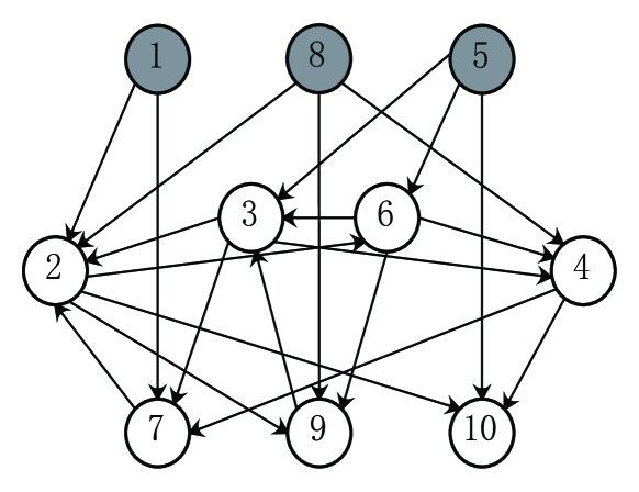
Figure 1: A fixed communication topology where $1$, $5$ and $8$ are faulty nodes, and the rest normal nodes are rooted.

\psfrag{CostFunction}[0.7]{$V(\mathbf{x}(k))$}\psfrag{Iteration}[0.7]{Iteration}\includegraphics[width=520.34267pt]{fixed.eps}

Figure 2: Reaching resilient consensus for normal nodes using WLA-F.

\psfrag{Iteration}[0.7]{Average Convergence Number}\psfrag{rate}[0.7]{Fault Probability}\includegraphics[width=520.34267pt]{secreterrorrate.eps}

Figure 3: The average convergence count varies with fault probability.

Next, we focus on the case of $3$ IFNs. In the above simulation, we define that the fault probability of each IFN is $1-p=0.2$. By increasing this fault probability from $0$ to $1$ for each IFN, with each round repeated $5000$ times, the average convergence count is described in Fig. 3 where the metric $V$ smaller than $5$ (half noise upper bound) is defined as convergence achievement. From the simulation results, the convergence count grows with increasing fault probability. More specifically, it grows fast with increasing fault probability at the range $[0,0.2]$, and keeps flat during $[0.2,0.8]$, and then continues to grow. This phenomenon is due to the reason that small probability fault (occasional faulty behavior) behind normal actions is more easily to be identified, and adjacent weight from faulty nodes continues to drop with slightly slower speed when fault probability increases.

5.1.2 Stochastic Topology Case

In the following, we assume that all nodes connect with each other in probability $0.5$ at each step. Thus, the topology is rooted in probability one. We define the parameter $\gamma=0.8$. We update the adjacent weights by WLA-S, then the result presented in Fig. 4 again validates our algorithm. The adjacent weight after $1000$ iterations is given in Table I showing that the adjacent weight from faulty nodes is quite small compared to the ones from normal nodes. It should be noted that the column sum may be greater than $1$, since for each node $i$, the weight sum of its connected neighbors’ at last iteration equals $0.8$, and all the other weight values are kept since last connected time. Again, it validates that IFNs can be more easily identified than PFNs.

\psfrag{CostFunction}[0.7]{$V(\mathbf{x}(k))$}\psfrag{Iteration}[0.7]{Iteration}\includegraphics[width=520.34267pt]{stochastic.eps}

Figure 4: Reaching resilient consensus for normal nodes using WLA-S.

Table 1: Adjacent Weight

	2	3	4	6	7	9	10
1	$\mathbf{0.019}$	$\mathbf{0.027}$	$\mathbf{0.021}$	$\mathbf{0.040}$	$\mathbf{0.027}$	$\mathbf{0.020}$	$\mathbf{0.027}$
2	$0$	$0.256$	$0.190$	$0.325$	$0.229$	$0.191$	$0.261$
3	$0.177$	$0$	$0.167$	$0.393$	$0.261$	$0.197$	$0.249$
4	$0.152$	$0.256$	$0$	$0.373$	$0.249$	$0.189$	$0.258$
5	$\mathbf{0.021}$	$\mathbf{0.031}$	$\mathbf{0.026}$	$\mathbf{0.041}$	$\mathbf{0.029}$	$\mathbf{0.026}$	$\mathbf{0.030}$
6	$0.142$	$0.269$	$0.191$	$0$	$0.241$	$0.186$	$0.261$
7	$0.163$	$0.276$	$0.200$	$0.373$	$0$	$0.206$	$0.267$
8	$\mathbf{0.007}$	$\mathbf{0.009}$	$\mathbf{0.008}$	$\mathbf{0.011}$	$\mathbf{0.009}$	$\mathbf{0.009}$	$\mathbf{0.012}$
9	$0.153$	$0.257$	$0.199$	$0.333$	$0.199$	$0$	$0.239$
10	$0.169$	$0.255$	$0.190$	$0.375$	$0.225$	$0.197$	$0$

In addition, we consider a large-scale network composed of $1000$ nodes, and the fault probability of IFN is $0.2$. By increasing the IFN number from $1$ to $500$ with each round repeated $1000$ times, the simulation results manifest that the normal nodes achieve resilient consensus by a large majority. This is due to the the reason that once abnormal behavior from IFN is recognized (large relative state), the corresponding reward and credibility are decreased and thus arduous to be promoted. This result indicates that our algorithms work well in large-scale networks.

5.2 Clock Synchronization

In this subsection, we apply our approach in a clock synchronization problem. We follow the example in [13], in which a sensor network consists of $16$ nodes including $2$ PFNs and $2$ IFNs. The undirected communication topology is shown in Fig. 5 such that the MSR algorithms are not available. The clock skew $\alpha^{*}_{i}$ and offset $\beta^{*}_{i}$ are randomly initialized within the intervals $[0.7,1.3]$ and $[0,100]$, respectively. The noise upper bound is restrict as $5$. To simplicity of experiment, the updating time instant is set $1$. The initial parameter $\alpha_{i}(0)=1$ and $\beta_{i}(0)=0.1$ for all $i$. The probability density functions $f_{\rm Random}$ for $\alpha$ and $\beta$ in PFN follow a continuous uniform distribution over the ranges $[0,5]$ and $[0,50]$, respectively. The logical clock demonstration without and with WLA are shown in Fig. 6 and Fig. 7, respectively, indicating resilient clock synchronization can be achieved by our approach, i.e., the logical clock difference between normal nodes is bounded.

Figure 5: A fixed communication topology where $2$, $6$, $8$ and $12$ are faulty nodes, and the rest normal nodes are rooted.

\psfrag{tau}[0.8]{$\tau$}\psfrag{Iteration}[0.7]{Iteration}\includegraphics[width=520.34267pt]{unclock.eps}

Figure 6: Divergent phenomenon of a group of normal nodes caused by faulty nodes without using WLA.

\psfrag{tau}[0.8]{$\tau$}\psfrag{Iteration}[0.7]{Iteration}\includegraphics[width=520.34267pt]{clock.eps}

Figure 7: Reaching resilient clock synchronization for each normal node using WLA-F with fixed communication connection.

6 Conclusions

In this paper, we present WLA to solve the resilient multi-agent consensus problem in the presence of noise and faulty nodes. Through defining a reward function by relative neighbor nodes’ states, adjusting the corresponding credibility and adjacent weights, the normal nodes finally achieve resilient consensus with reducing the weights from faulty nodes to sufficiently small values. In our study, two types of faulty behavior models and two types of network topology are considered. Moreover, the proposed approach is applied in a clock synchronization problem such that hacked or malfunctioning nodes can be gradually ignored. By our algorithms, the network condition is greatly relaxed and only one-step information is required. In the future, we will consider the cooperation among the faulty nodes and more applications in, e.g., beamforming technology and social networks.

References

- [1] P. Guo, W. Hou, L. Guo, W. Sun, C. Liu, H. Bao, L. Duong, and W. Liu. Fault-tolerant routing mechanism in 3d optical network-on-chip based on node reuse. IEEE Transactions on Parallel and Distributed Systems, 2019.
- [2] S. Sundaram and C. N. Hadjicostis. Distributed function calculation via linear iterative strategies in the presence of malicious agents. IEEE Transactions on Automatic Control, 56(7):1495–1508, 2011.
- [3] F. Pasqualetti, A. Bicchi, and F. Bullo. Consensus computation in unreliable networks: A system theoretic approach. IEEE Transactions on Automatic Control, 57(1):90–104, 2012.
- [4] H. J. LeBlanc and X. D. Koutsoukos. Consensus in networked multi-agent systems with adversaries. In Proceedings of the 14th ACM International Conference on Hybrid Systems: Computation and Control, pages 281–290, Chicago, IL, USA, 2011.
- [5] H. J. LeBlanc and X. D. Koutsoukos. Low complexity resilient consensus in networked multi-agent systems with adversarie. In Proceedings of the 15th ACM International Conference on Hybrid Systems: Computation and Control, pages 5–14, Beijing, China, 2012.
- [6] S. M. Dibaji and H. Ishii. Resilient consensus of second-order agent networks: Asynchronous update rules over robust graphs. Automatica, 81:123–132, 2017.
- [7] N. H. Vaidya, L. Tseng, , and G. Liang. Iterative approximate byzantine consensus in arbitrary directed graphs. In Proceedings of the 2012 ACM Symposium on Principles of Distributed Computing, pages 365–374, Madeira, Portugal, 2012.
- [8] H. J. LeBlanc, H. Zhang, X. Koutsoukos, and S. Sundaram. Resilient asymptotic consensus in robust networks. IEEE Journal on Selected Areas in Communications, 31(4):766–781, 2013.
- [9] D. G. Mikulski, F. L. Lewis, E. Y. Gu, and G. R. Hudas. Trust method for multi-agent consensus. In Conference on Unmanned Systems Technology XIV, pages 1–15, Baltimore, MD, USA, 2012.
- [10] X. Liu and J. S. Baras. Using trust in distributed consensus with adversaries in sensor and other networks. In Proceedings of the 2014 International Conference on Information Fusion, pages 1–7, Salamanca, Spain, 2014.
- [11] J. Wang, L. Zhao, J. Liu, and N. Kato. Smart resource allocation for mobile edge computing: a deep reinforcement learning approach. IEEE Transactions on Emerging Topics in Computing, 2019.
- [12] H. M. Schwartz. Multi-Agent Machine Learning: A Reinforcement Approach. John Wiley Sons, 2014.
- [13] Y. Kikuya, S. M. Dibaji, and H. Ishii. Fault-tolerant clock synchronization over unreliable channels in wireless sensor networks. IEEE Transactions on Control of Network Systems, 5(4):1551–1562, 2017.
- [14] J. Elson, L. Girod, and D. Estrin. Fine-grained network time synchronization using reference broadcasts. In ACM SIGOPS Operating Systems Review, pages 147–163, 2002.
- [15] S. Ganeriwal, R. Kumar, and M. B. Srivastava. Timing-sync protocol for sensor networks. In Proceedings of the 1st international conference on Embedded networked sensor systems, pages 138–149, Los Angeles, California, USA, 2003.
- [16] D. Huang, W. Teng, and K. Yang. Secured flooding time synchronization protocol with moderator. International Journal of Communication Systems, 26(9):1092–1115, 2013.
- [17] L. Schenato and F. Fiorentin. Average timesynch: A consensus-based protocol for clock synchronization in wireless sensor networks. Automatica, 47(9):1878–1886, 2011.
- [18] J. He, P. Cheng, L. Shi, J. Chen, and Y. Sun. Time synchronization in wsns: A maximum-value-based consensus approach. IEEE Transactions on Automatic Control, 59(3):660–675, 2013.
- [19] R. Carli and S. Zampieri. Network clock synchronization based on the second-order linear consensus algorithm. IEEE Transactions on Automatic Control, 59(2):409–422, 2013.
- [20] J. He, X. Duan, P. Cheng, L. Shi, and L. Cai. Accurate clock synchronization in wireless sensor networks with bounded noise. Automatica, 81:350–358, 2017.
- [21] J. Hou and R. Zheng. Hierarchical consensus problem via group information exchange. IEEE Transactions on Cybernetics, 99:1–7, 2018.
- [22] A. Koppel, B. M. Sadler, and A. Ribeiro. Proximity without consensus in online multiagent optimization. IEEE Transactions on Signal Processing, 65(12):3062–3077, 2017.
- [23] V. D. Blondel, J. M. Hendrickx, A. Olshevsky, and J. N. Tsitsiklis. Convergence in multiagent coordination, consensus and flocking. In Procceedings of the 44th IEEE Conference on Decision and Control, and the European Control Conference, pages 2996–3000, Seville, Spain, 2005.