Self-Attentive Associative Memory

Abstract

Heretofore, neural networks with external memory are restricted to single memory with lossy representations of memory interactions. A rich representation of relationships between memory pieces urges a high-order and segregated relational memory. In this paper, we propose to separate the storage of individual experiences (item memory) and their occurring relationships (relational memory). The idea is implemented through a novel Self-attentive Associative Memory (SAM) operator. Found upon outer product, SAM forms a set of associative memories that represent the hypothetical high-order relationships between arbitrary pairs of memory elements, through which a relational memory is constructed from an item memory. The two memories are wired into a single sequential model capable of both memorization and relational reasoning. We achieve competitive results with our proposed two-memory model in a diversity of machine learning tasks, from challenging synthetic problems to practical testbeds such as geometry, graph, reinforcement learning, and question answering.

1 Introduction

Humans excel in remembering items and the relationship between them over time (Olson et al., 2006; Konkel & Cohen, 2009). Numerous neurocognitive studies have revealed this striking ability is largely attributed to the perirhinal cortex and hippocampus, two brain regions that support item memory (e.g., objects, events) and relational memory (e.g., locations of objects, orders of events), respectively (Cohen et al., 1997; Buckley, 2005). Relational memory theory posits that there exists a representation of critical relationships amongst arbitrary items, which allows inferential reasoning capacity (Eichenbaum, 1993; Zeithamova et al., 2012). It remains unclear how the hippocampus can select the stored items in clever ways to unearth their hidden relationships and form the relational representation.

Research on artificial intelligence has focused on designing item-based memory models with recurrent neural networks (RNNs) (Hopfield, 1982; Elman, 1990; Hochreiter & Schmidhuber, 1997) and memory-augmented neural networks (MANNs) (Graves et al., 2014, 2016; Le et al., 2018a, 2019). These memories support long-term retrieval of previously seen items yet lack explicit mechanisms to represent arbitrary relationships amongst the constituent pieces of the memories. Recently, further attempts have been made to foster relational modeling by enabling memory-memory interactions, which is essential for relational reasoning tasks (Santoro et al., 2017, 2018; Vaswani et al., 2017). However, no effort has been made to model jointly item memory and relational memory explicitly.

We argue that dual memories in a single system are crucial for solving problems that require both memorization and relational reasoning. Consider graphs wherein each node is associated with versatile features– as example a road network structure where each node is associated with diverse features: graph 1 where the nodes are building landmarks and graph 2 where the nodes are flora details. The goal here is to reason over the structure and output the associated features of the nodes instead of the pointer or index to the nodes. Learning to output associated node features enables generalization to entirely novel features, i.e., a model can be trained to generate a navigation path with building landmarks (graph 1) and tested in the novel context of generating a navigation path with flora landmarks (graph 2). This may be achieved if the model stores the features and structures into its item and relational memory, separately, and reason over the two memories using rules acquired during training.

Another example requiring both item and relational memory can be understood by amalgamating the $N^{th}$-farthest (Santoro et al., 2018) and associative recall (Graves et al., 2014) tasks. $N^{th}$-farthest requires relational memory to return a fixed one-hot encoding representing the index to the $N^{th}$-farthest item, while associative recall returns the item itself, requiring item memory. If these tasks are amalgamated to compose Relational Associative Recall (RAR) – return the $N^{th}$-farthest item from a query (see $\mathsection$ 3.2), it is clear that both item and relational memories are required.

Three limitations of the current approaches are: $\left(i\right)$ the relational representation is often computed without storing, which prevents reusing the precomputed relationships in sequential tasks (Vaswani et al., 2017; Santoro et al., 2017), $\left(ii\right)$ few works that manage both items and the relationships in a single memory, make it hard to understand how relational reasoning occurs (Santoro et al., 2018; Schlag & Schmidhuber, 2018), $\left(iii\right)$ the memory-memory relationship is coarse since it is represented as either dot product attention (Vaswani et al., 2017) or weighted summation via neural networks (Santoro et al., 2017). Concretely, the former uses a scalar to measure cosine distance between two vectors and the later packs all information into one vector via only additive interactions.

To overcome the current limitations, we hypothesize a two-memory model, in which the relational memory exists separately from the item memory. To maintain a rich representation of the relationship between items, the relational memory should be higher-order than the item memory. That is, the relational memory stores multiple relationships, each of which should be represented by a matrix rather than a scalar or vector. Otherwise, the capacity of the relational memory is downgraded to that of the item memory. Finally, as there are two separate memories, they must communicate to enrich the representation of one another.

To implement our hypotheses, we introduce a novel operator that facilitates the communication from the item memory to the relational memory. The operator, named Self-attentive Associative Memory (SAM) leverages the dot product attention with our outer product attention. Outer product is critical for constructing higher-order relational representations since it retains bit-level interactions between two input vectors, thus has potential for rich representational learning (Smolensky, 1990). SAM transforms a second-order (matrix) item memory into a third-order relational representation through two steps. First, SAM decodes a set of patterns from the item memory. Second, SAM associates each pair of patterns using outer product and sums them up to form a hetero-associative memory. The memory thus stores relationships between stored items accumulated across timesteps to form a relational memory.

The role of item memory is to memorize the input data over time. To selectively encode the input data, the item memory is implemented as a gated auto-associative memory. Together with previous read-out values from the relational memory, the item memory is used as the input for SAM to construct the relational memory. In return, the relational memory transfers its knowledge to the item memory through a distillation process. The backward transfer triggers recurrent dynamics between the two memories, which may be essential for simulating hippocampal processes (Kumaran & McClelland, 2012). Another distillation process is used to transform the relational memory to the output value.

Taken together, we contribute a new neural memory model dubbed SAM-based Two-memory Model (STM) that takes inspiration from the existence of both item and relational memory in human brain (Konkel & Cohen, 2009). In this design, the relational memory is higher-order than the item memory and thus necessitates a core operator that manages the information exchange from the item memory to the relational memory. The operator, namely Self-attentive Associative Memory (SAM), utilizes outer product to construct a set of hetero-associative memories representing relationships between arbitrary stored items. We apply our model to a wide range of tasks that may require both item and relational memory: various algorithmic learning, geometric and graph reasoning, reinforcement learning and question-answering tasks. Several analytical studies on the characteristics of our proposed model are also given in the Appendix.

2 Methods

2.1 Outer product attention (OPA)

Outer product attention (OPA) is a natural extension of the query-key-value dot product attention (Vaswani et al., 2017). Dot product attention (DPA) for single query $q$ and $n_{kv}$ pairs of key-value can be formulated as follows,

$$A^{\text{\textdegree}}\left(q,K,V\right)=\sum_{i=1}^{n_{kv}}\mathcal{S}\left(q\cdot k_{i}\right)v_{i}$$ (1)

where $A^{\text{\textdegree}}\in\mathbb{R}^{d_{v}}$, $q,k_{i}\in\mathbb{R}^{d_{qk}}$, $v_{i}\in\mathbb{R}^{d_{v}}$, $\cdot$ is dot product, and $\mathcal{\mathcal{S}}$ forms $\mathrm{softmax}$ function. We propose a new outer product attention with similar formulation yet different meaning,

$$A^{\otimes}\left(q,K,V\right)=\sum_{i=1}^{n_{kv}}\mathcal{F}\left(q\odot k_{i}\right)\otimes v_{i}$$ (2)

where $A^{\otimes}\in\mathbb{R}^{d_{qk}\times d_{v}}$, $q,k_{i}\in\mathbb{R}^{d_{qk}}$, $v\in\mathbb{R}^{d_{v}}$, $\odot$ is element-wise multiplication, $\otimes$ is outer product and $\mathcal{F}$ is chosen as element-wise $\tanh$ function.

A crucial difference between DPA and OPA is that while the former retrieves an attended item $A^{\text{\textdegree}}$, the latter forms a relational representation $A^{\otimes}$. As a relational representation, $A^{\otimes}$ captures all bit-level associations between the key-scaled query and the value. This offers two benefits: $\left(i\right)$ a higher-order representational capacity that DPA cannot provide and $\left(ii\right)$ a form of associative memory that can be later used to retrieve stored item by using a contraction operation $\mathcal{P}\left(A^{\otimes}\right)$ (see Appendix $\mathsection$ C-Prop. 6).

OPA is closely related to DPA. The relationship between the two for simple $\mathcal{S}$ and $\mathcal{F}$ is presented as follows,

Proposition 1.

Assume that $\mathcal{\mathcal{S}}$ is a linear transformation: $\mathcal{S}\left(x\right)=ax+b$ ($a,b,x\in\mathbb{R}$), we can extract $A^{\text{\textdegree}}$ from $A^{\otimes}$ by using an element-wise linear transformation $\mathcal{F}\left(x\right)=a^{f}\odot x+b^{f}$ ($a^{f},b^{f},x\in\mathbb{R}^{d_{qk}}$) and a contraction $\mathcal{P}$: $\mathbb{R}^{d_{qk}\times d_{v}}\rightarrow\mathbb{R}^{d_{v}}$ such that

$$A^{\text{\textdegree}}\left(q,K,V\right)=\mathcal{P}\left(A^{\otimes}\left(q,K,V\right)\right)$$ (3)

Proof.

see Appendix $\mathsection$ A. ∎

Moreover, when $n_{kv}=1$, applying a high dimensional transformation $\mathcal{G}\left(A^{\otimes}\right)$ is equivalent to the well-known bi-linear model (see Appendix $\mathsection$ B-Prop. 4). By introducing OPA, we obtain a new building block that naturally supports both powerful relational bindings and item memorization.

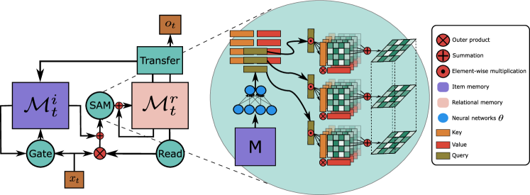
Figure 1: STM (left) and SAM (right). SAM uses neural networks $\theta$ to extract query, key and value elements from a matrix memory $M$. In this illustration, $n_{q}=3$ and $n_{kv}=4$. Then, it applies outer product attention to output a $3D$ tensor relational representation. In STM, at every timestep, the item memory $\mathcal{M}_{t}^{i}$ is updated with new input $x_{t}$ using gating mechanisms (Eq. 10). The item memory plus the read-out from the relational memory is forwarded to SAM, resulting in a new relational representation to update the relational memory $\mathcal{M}_{t}^{r}$ (Eq. 11-12). The relational memory transfers its knowledge to the item memory (Eq. 13) and output value (Eq. 14).

2.2 Self-attentive Associative Memory (SAM)

We introduce a novel and generic operator based upon OPA that constructs relational representations from an item memory. The relational information is extracted via preserving the outer products between any pairs of items from the item memory. Hence, we name this operator Self-attentive Associative Memory (SAM). Given an item memory $M\in\mathbb{R}^{n\times d}$ and parametric weights $\text{$\theta$=}\left\{W_{q}\in\mathbb{R}^{n_{q}\times n}\right.$, $W_{k}\in\mathbb{R}^{n_{kv}\times n}$, $\left.W_{v}\in\mathbb{R}^{n_{kv}\times n}\right\}$, SAM retrieves $n_{q}$ queries, $n_{kv}$ keys and values from $M$ as $M_{q}$, $M_{k}$ and $M_{v}$, respectively,

$$M_{q}=\mathcal{LN}\left(W_{q}M\right)$$ (4)

$$M_{k}=\mathcal{LN}\left(W_{k}M\right)$$ (5)

$$M_{v}=\mathcal{LN}\left(W_{v}M\right)$$ (6)

where $\mathcal{LN}$ is layer normalization operation (Ba et al., 2016b). Then SAM returns a relational representation $\mathrm{SAM}_{\theta}\left(M\right)$$\in\mathbb{R}^{n_{q}\times d\times d}$, in which the $s$-th element of the first dimension is defined as

$$\mathrm{SAM}_{\theta}\left(M\right)\left[s\right] =A^{\otimes}\left(M_{q}\left[s\right],M_{k},M_{v}\right)$$ (7)

$$=\sum_{j=1}^{n_{kv}}\mathcal{F}\left(M_{q}\left[s\right]\odot M_{k}\left[j\right]\right)\otimes M_{v}\left[j\right]$$ (8)

where $s=1,...,n_{q}$. $M_{q}\left[s\right]$, $M_{k}\left[j\right]$ and $M_{v}\left[j\right]$ denote the $s$-th row vector of matrix $M_{q}$, the $j$-th row vector of matrix $M_{k}$ and $M_{v}$, respectively. A diagram illustrating SAM operations is given in Fig. 1 (right).

It should be noted that $M$ can be any item memory including the slot-based memories (Le et al., 2019), direct inputs (Vaswani et al., 2017) or associative memories (Kohonen, 1972; Hopfield, 1982). We choose $M\in\mathbb{R}^{d\times d}$ as a form of classical associative memory, which is biologically plausible (Marr & Thach, 1991). Here, we follow the traditional practice that sets $n=d$ for the associative item memory. From $M$ we read query, key and value items to form $\mathrm{SAM}_{\theta}\left(M\right)$–a new set of hetero-associative memories using Eq. 8. Each hetero-associative memory represents the relationship between a query and all values. The role of the keys is to maintain possible perfect retrieval for the item memory (Appendix $\mathsection$ C-Prop. 6).

The high-order structure of SAM allows it to preserve bit-level relationships between a query and a value in a matrix. SAM compresses several relationships with regard to a query by summing all the matrices to form a hetero-associative memory containing $d^{2}$ scalars, where $d$ is the dimension of $M$. As there are $n_{kv}$ relationships given 1 query, the summation results in on average $d^{2}/n_{kv}$ scalars of representation per relationship, which is greater than $1$ if $d>\sqrt{n_{kv}}$. By contrast, current self-attention mechanisms use dot product to measure the relationship between any pair of memory slots, which means 1 scalar per relationship.

2.3 SAM-based Two-Memory Model (STM)

To effectively utilize the SAM operator, we design a system which consists of two memory units $\mathcal{M}_{t}^{i}\in\mathbb{R}^{d\times d}$ and $\mathcal{M}_{t}^{r}\in\mathbb{R}^{n_{q}\times d\times d}$: one for items and the other for relationships, respectively. From a high-level view, at each timestep, we use the current input data $x_{t}$ and the previous state of memories $\left\{\mathcal{M}_{t-1}^{i},\mathcal{M}_{t-1}^{r}\right\}$ to produce output $o_{t}$ and new state of memories $\left\{\mathcal{M}_{t}^{i},\mathcal{M}_{t}^{r}\right\}$. The memory executions are described as follows.

$\mathcal{M}^{i}$-Write

The item memory distributes the data from the input across its rows in the form of associative memory. For an input $x_{t}$, we update the item memory as

$$X_{t} =f_{1}\left(x_{t}\right)\otimes f_{2}\left(x_{t}\right)$$

$$\mathcal{M}_{t}^{i} =\mathcal{M}_{t-1}^{i}+X_{t}$$ (9)

where $f_{1}$ and $f_{2}$ are feed-forward neural networks that output $d$-dimensional vectors. This update does not discriminate the input data and inherits the low-capacity of classical associative memory (Rojas, 2013). We leverage the gating mechanisms of LSTM (Hochreiter & Schmidhuber, 1997) to improve Eq. 9 as

$$\mathcal{M}_{t}^{i}=F_{t}\left(\mathcal{M}_{t-1}^{i},x_{t}\right)\odot\mathcal{M}_{t-1}^{i}+I_{t}\left(\mathcal{M}_{t-1}^{i},x_{t}\right)\odot X_{t}$$ (10)

where $F_{t}$ and $I_{t}$ are forget and input gates, respectively. Detailed implementation of these gates is in Appendix $\mathsection$ D.

$\mathcal{M}^{r}$-Read

As relationships stored in $\mathcal{M}^{r}$ are represented as associative memories, the relational memory can be read to reconstruct previously seen items. As shown in Appendix $\mathsection$ C-Prop. 7, the read is basically a two-step contraction,

$$v_{t}^{r}=\mathrm{softmax}\left(f_{3}\left(x_{t}\right)^{\top}\right)\mathcal{M}_{t-1}^{r}f_{2}\left(x_{t}\right)$$ (11)

where $f_{3}$ is a feed-forward neural network that outputs a $n_{q}$-dimensional vector. The read value provides an additional input coming from the previous state of $\mathcal{M}^{r}$ to relational construction process, as shown later in Eq. 12.

$\mathcal{M}^{i}$-Read $\mathcal{M}^{r}$-Write

We use SAM to read from $\mathcal{M}^{i}$ and construct a candidate relational memory, which is simply added to the previous relational memory to perform the relational update,

$$\mathcal{M}_{t}^{r}=\mathcal{M}_{t-1}^{r}+\alpha_{1}\mathrm{SAM}_{\theta}\left(\mathcal{M}_{t}^{i}+\alpha_{2}v_{t}^{r}\otimes f_{2}\left(x_{t}\right)\right)$$ (12)

where $\alpha_{1}$and $\alpha_{2}$ are blending hyper-parameters. The input for SAM is a combination of the current item memory $\mathcal{M}_{t}^{i}$ and the association between the extracted item from the previous relational memory $v_{t}^{r}$ and the current input data $x_{t}$. Here, $v_{t}^{r}$ enhances the relational memory with information from the distant past. The resulting relational memory stores associations between several pairs of items in a $3D$ tensors of size $n_{q}\times d\times d$. In our SAM implementation, $n_{kv}=n_{q}$.

$\mathcal{M}^{r}$-Transer

In this phase, the relational knowledge from $\mathcal{M}_{t}^{r}$ is transferred to the item memory by using high dimensional transformation,

$$\mathcal{M}_{t}^{i}=\mathcal{M}_{t}^{i}+\alpha_{3}\mathcal{G}_{1}\circ\mathcal{V}_{f}\circ\mathcal{M}_{t}^{r}$$ (13)

where $\mathcal{V}_{f}$ is a function that flattens the first two dimensions of its input tensor, $\mathcal{G}_{1}$ is a feed-forward neural network that maps $\mathbb{R}^{\left(n_{q}d\right)\times d}\rightarrow\mathbb{R}^{d\times d}$ and $\alpha_{3}$ is a blending hyper-parameter. As shown in Appendix $\mathsection$ B-Prop. 5, with trivial $\mathcal{G}_{1}$, the transfer behaves as if the item memory is enhanced with long-term stored values from the relational memory. Hence, $\mathcal{M}^{r}$-Transfer is also helpful in supporting long-term recall (empirical evidences in $\mathsection$ 3.1). In addition, at each timestep, we distill the relational memory into an output vector $o_{t}\in\mathbb{R}^{n_{o}}$. We alternatively flatten and apply high-dimensional transformations as follow,

$$o_{t}=\mathcal{G}_{3}\circ\mathcal{V}_{l}\circ\mathcal{G}_{2}\circ\mathcal{V}_{l}\circ\mathcal{M}_{t}^{r}$$ (14)

where $\mathcal{V}_{l}$ is a function that flattens the last two dimensions of its input tensor. $\mathcal{G}_{2}$ and $\mathcal{G}_{3}$ are two feed-forward neural networks that map $\mathbb{R}^{n_{q}\times\left(dd\right)}\rightarrow\mathbb{R}^{n_{q}\times n_{r}}$ and $\mathbb{R}^{n_{q}n_{r}}\rightarrow\mathbb{R}^{n_{o}}$, respectively. $n_{r}$ is a hyper-parameter.

Unlike the contraction (Eq. 11), the distillation process does not simply reconstruct the stored items. Rather, thanks to high-dimensional transformations, it captures bi-linear representations stored in the relational memory (proof in Appendix $\mathsection$ B). Hence, despite its vector form, the output of our model holds a rich representation that is useful for both sequential and relational learning. We discuss further on how to quantify the degree of relational distillation in Appendix $\mathsection$ G. The summary of components of STM is presented in Fig. 1 (left).

3 Results

3.1 Ablation study

We test different model configurations on two classical tasks for sequential and relational learning: associative retrieval (Ba et al., 2016a) and $N^{th}$-farthest (Santoro et al., 2018) (see Appendix $\mathsection$ E for task details and learning curves). Our source code is available at https://github.com/thaihungle/SAM.

Associative retrieval

This task measures the ability to recall a seen item given its associated key and thus involves item memory. We use the setting with input sequence length 30 and 50 (Zhang & Zhou, 2017). Three main factors affecting the item memory of STM are the dimension $d$ of the auto-associative item memory, the gating mechanisms (Eq. 10) and the relational transfer (Eq. 13). Hence, we ablate our STM ($d=96$, full features) by creating three other versions: small STM with transfer ($d=48$), small STM without transfer ($d=48$, w/o transfer) and STM without gates ($d=96$, w/o gates). $n_{q}$ is fixed to $1$ as the task does not require much relational learning.

Table 1 reports the number of epochs required to converge and the final testing accuracy. Without the proposed gating mechanism, STM struggles to converge, which highlights the importance of extending the capacity of the auto-associative item memory. The convergence speed of STM is significantly improved with a bigger item memory size. Relational transfer seems more useful for longer input sequences since if requested, it can support long-term retrieval. Compared to other fast-weight baselines, the full-feature STM performs far better as it needs only 10 and 20 epochs to solve the tasks of length 30 and 50, respectively.

Model	Length 30		Length 50
	E.	A.	E.	A.
Fast weight∗	50	100	5000	20.8
WeiNet∗	35	100	50	100
STM ($d=48$, w/o transfer)	10	100	100	100
STM ($d=48$)	20	100	80	100
STM ($d=96$, w/o gates)	100	24	100	20
STM ($d=96$)	10	100	20	100

Table 1: Comparison of models on associative retrieval task with number of epochs E. required to converge (lower is better) and convergence test accuracy A. ($\%$, higher is better). $*$ is reported from Zhang & Zhou (2017).

$\boldsymbol{N^{th}}$-farthest

This task evaluates the ability to learn the relationship between stored vectors. The goal is to find the $N^{th}$-farthest vector from a query vector, which requires a relational memory for distances between vectors and a sorting mechanism over the distances. For relational reasoning tasks, the pivot is the number of extracted items $n_{q}$ for establishing the relational memory. Hence, we run our STM with different $n_{q}=1,4,8$ using the same problem setting (8 $16$- dimensional input vectors), optimizer (Adam), batch size (1600) as in Santoro et al. (2018). We also run the task with TPR (Schlag & Schmidhuber, 2018)–a high-order fast-weight model that is designed for reasoning.

As reported in Table 2, increasing $n_{q}$ gradually improves the accuracy of STM. As there are 8 input vectors in this task, literally, at each timestep the model needs to extract 8 items to compute all pairs of distances. However, as the extracted item is an entangled representation of all stored vectors and the temporarily computed distances are stored in separate high-order storage, even with $n_{q}=1,4$, STM achieves moderate results. With $n_{q}=8$, STM nearly solves the task perfectly, outperforming RMC by a large margin. We have tried to tune TPR for this task without success (see Appendix $\mathsection$ E). This illustrates the challenge of training high-order neural networks in diverse contexts.

Model	Accuracy ($\%$)
DNC∗	25
RMC∗	91
TPR	13
STM ($n_{q}=1$)	84
STM ($n_{q}=4$)	95
STM ($n_{q}=8$)	98

Table 2: Comparison of models on $N^{th}$-farthest task (test accuracy). $*$ is reported from Santoro et al. (2018).

3.2 Algorithmic synthetic tasks

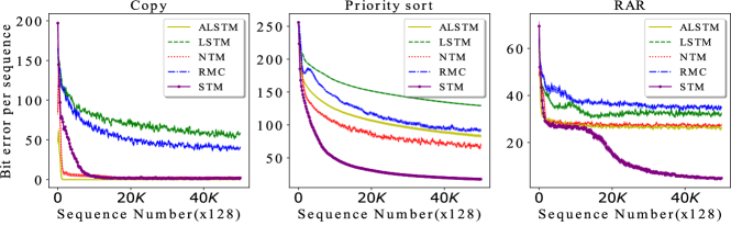
Figure 2: Bit error per sequence vs training iteration for algorithmic synthetic tasks.

Algorithmic synthetic tasks (Graves et al., 2014) examine sequential models on memorization capacity (eg., Copy, Associative recall) and simple relational reasoning (eg., Priority sort). Even without explicit relational memory, MANNs have demonstrated good performance (Graves et al., 2014; Le et al., 2020), but they are verified for only low-dimensional input vectors (<8 bits). As higher-dimensional inputs necessitate higher-fidelity memory storage, we evaluate the high-fidelity reconstruction capacity of sequential models for these algorithmic tasks with 32-bit input vectors.

Two chosen algorithmic tasks are Copy and Priority sort. Item memory is enough for Copy where the models just output the input vectors seen in the same order in which they are presented. For Priority sort, a relational operation that compares the priority of input vectors is required to produce the seen input vectors in the sorted order according to the priority score attached to each input vector. The relationship is between input vectors and thus simply first-order (see Appendix $\mathsection$ G for more on the order of relationship).

Inspired by Associative recall and $N^{th}$-farthest tasks, we create a new task named Relational Associative Recall (RAR). In RAR, the input sequence is a list of items followed by a query item. Each item is a list of several 32-bit vectors and thus can be interpreted as a concatenated long vector. The requirement is to reconstruct the seen item that is farthest or closest (yet unequal) to the query. The type of the relationship is conditioned on the last bit of the query vector, i.e., if the last bit is 1, the target is the farthest and 0 the closest. The evaluated models must compute the distances from the query item to any other seen items and then compare the distances to find the farthest/closest one. Hence, this task is similar to the $N^{th}$-farthest task, which is second-order relational and thus needs relational memory. However, this task is more challenging since the models must reconstruct the seen items (32-bit vectors). Compared to $N=8$ possible one-hot outputs in $N^{th}$-farthest, the output space in RAR is $2^{32}$ per step, thereby requiring high-fidelity item memory.

We evaluate our model STM ($n_{q}=8$, $d=96$) with the 4 following baselines: LSTM (Hochreiter & Schmidhuber, 1997), attentional LSTM (Bahdanau et al., 2015), NTM (Graves et al., 2014) and RMC (Santoro et al., 2018). Details of the implementation are listed in Appendix $\mathsection$ F. The learning curves (mean and error bar over 5 runs) are presented in Fig. 2.

LSTM is often the worst performer as it is based on vector memory. ALSTM is especially good for Copy as it has a privilege to access input vectors at every step of decoding. However, when dealing with relational reasoning, memory-less attention in ALSTM does not help much. NTM performs well on Copy and moderately on Priority sort, yet badly on RAR possibly due to its bias towards item memory. Although equipped with self-attention relational memory, RMC demonstrates trivial performance on all tasks. This suggests a limitation of using dot-product attention to represent relationships when the tasks stress memorization or the relational complexity goes beyond dot-product capacity. Amongst all models, only the proposed STM demonstrates consistently good performance where it almost achieves zero errors on these 3 tasks. Notably, for RAR, only STM can surpass the bottleneck error of 30 bits and reach $\approx 1$ bit error, corresponding to 0% and 87% of items perfectly reconstructed, respectively.

Model	#Parameters	Convex hull		TSP		Shortest	Minimum
		$N=5$	$N=10$	$N=5$	$N=10$	path	spanning tree
LSTM	4.5 M	89.15	82.24	73.15 (2.06)	62.13 (3.19)	72.38	80.11
ALSTM	3.7 M	89.92	85.22	71.79 (2.05)	55.51 (3.21)	76.70	73.40
DNC	1.9 M	89.42	79.47	73.24 (2.05)	61.53 (3.17)	83.59	82.24
RMC	2.8 M	93.72	81.23	72.83 (2.05)	37.93 (3.79)	66.71	74.98
STM	1.9 M	96.85	91.88	73.96 (2.05)	69.43 (3.03)	93.43	94.77

Table 3: Prediction accuracy ($\%$) for geometric and graph reasoning with random one-hot features. Italic numbers are tour length–additional metric for TSP. Average optimal tour lengths found by brute-force search for $N=5$ and $10$ are 2.05 and 2.88, respectively.

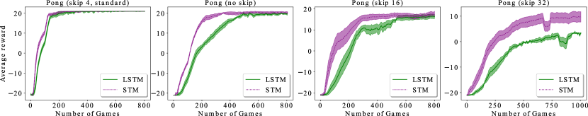
Figure 3: Average reward vs number of games for reinforcement learning task in n-frame skip settings.

3.3 Geometric and graph reasoning

Problems on geometry and graphs are a good testbed for relational reasoning, where geometry stipulates spatial relationships between points, and graphs the relational structure of nodes and edges. Classical problems include Convex hull, Traveling salesman problem (TSP) for geometry, and Shortest path, Minimum spanning tree for graph. Convex hull and TSP data are from Vinyals et al. (2015) where input sequence is a list of points’ coordinates (number of points $N\sim\left[5,20\right]$). Graphs in Shortest path and Minimum spanning tree are generated with solutions found by Dijkstra and Kruskal algorithms, respectively. A graph input is represented as a sequence of triplets $\left(node_{1},node_{2},edge_{12}\right)$. The desired output is a sequence of associated features of the solution points/nodes (more in Appendix $\mathsection$ H).

We generate a random one-hot associated feature for each point/node, which is stacked into the input vector. This allows us to output the node’s associated features. This is unlike Vinyals et al. (2015), who just outputs the pointers to the nodes. Our modification creates a challenge for both training and testing. The training is more complex as the feature of the nodes varies even for the same graph. The testing is challenging as the associated features are likely to be different from that in the training. A correct prediction for a timestep is made when the predicted feature matches perfectly with the ground truth feature in the timestep. To measure the performance, we use the average accuracy of prediction across steps. We use the same baselines as in $\mathsection$ 3.2 except that we replace NTM with DNC as DNC performs better on graph reasoning (Graves et al., 2016).

We report the best performance of the models on the testing datasets in Table 3. Although our STM has fewest parameters, it consistently outperforms other baselines by a significant margin. As usual, LSTM demonstrates an average performance across tasks. RMC and ALSTM are only good at Convex hull. DNC performs better on graph-like problems such as Shortest path and Minimum spanning tree. For the NP-hard TSP ($N=5$), despite moderate point accuracy, all models achieve nearly minimal solutions with an average tour length of $2.05$. When increasing the difficulty with more points ($N=10$), none of these models reach an average optimal tour length of $2.88$. However, only STM approaches closer to the optimal solution without the need for pointer and beam search mechanisms. Armed with both item and relational memory, STM’s superior performance suggests a qualitative difference in the way STM and other methods solve these problems.

3.4 Reinforcement learning

Memory is helpful for partially observable Markov decision process (Bakker, 2002). We apply our memory to LSTM agents in Atari game environment using A3C training (Mnih et al., 2016). More details are given in Appendix $\mathsection$ I. In Atari games, each state is represented as the visual features of a video frame and thus is partially observable. To perform well, RL agents should remember and relate several frames to model the game state comprehensively. These abilities are challenged when over-sampling and under-sampling the observation, respectively. We analyze the performance of LSTM agents and their STM-augmented counterparts under these settings using a game: Pong.

To be specific, we test the two agents on different frame skips (0, 4, 16, 32). We create $n$-frame skip setting by allowing the agent to see the environment only after every $n$ frames, where 4-frame skip is standard in most Atari environments. When no frameskip is applied (over-sampling), the number of observations is dense and the game is long (up to 9000 steps per game), which requires high-capacity item memory. On the contrary, when a lot of frames are skipped (under-sampling), the observations become scarce and the agents must model the connection between frames meticulously, demanding better relational memory.

We run each configuration 5 times and report the mean and error bar of moving average reward (window size $=100$) through training time in Fig. 3. In a standard condition (4-frame skip), both baselines can achieve perfect performance and STM outperforms LSTM slightly in terms of convergence speed. The performance gain becomes clearer under extreme conditions with over-sampling and under-sampling. STM agents require fewer practices to accomplish higher rewards, especially in the 32-frame skip environment, which illustrates that having strong item and relational memory in a single model is beneficial to RL agents.

3.5 Question answering

bAbI is a question answering dataset that evaluates the ability to remember and reason on textual information (Weston et al., 2015). Although synthetically generated, the dataset contains 20 challenging tasks such as pathfinding and basic induction, which possibly require both item and relational memory. Following Schlag & Schmidhuber (2018), each story is preprocessed into a sentence-level sequence, which is fed into our STM as the input sequence. We jointly train STM for all tasks using normal supervised training (more in Appendix $\mathsection$ J). We compare our model with recent memory networks and report the results in Table 4.

MANNs such as DNC and NUTM have strong item memory, yet do not explicitly support relational learning, leading to significantly higher errors compared to other models. On the contrary, TPR is explicitly equipped with relational bindings but lack of item memory and thus clearly underperforms our STM. Universal Transformer (UT) supports a manually set item memory with dot product attention, showing higher mean error than STM with learned item memory and outer product attention. Moreover, our STM using normal supervised loss outperforms MNM-p trained with meta-level loss, establishing new state-of-the-arts on bAbI dataset. Notably, STM achieves this result with low variance, solving 20 tasks for 9/10 run (see Appendix $\mathsection$ J).

Model	Error
	Mean	Best
DNC (Graves et al., 2016)	12.8 $\pm$ 4.7	3.8
NUTM (Le et al., 2020)	5.6 $\pm$ 1.9	3.3
TPR (Schlag & Schmidhuber, 2018)	1.34 $\pm$ 0.52	0.81
UT (Dehghani et al., 2018)	1.12 $\pm$ 1.62	0.21
MNM-p (Munkhdalai et al., 2019)	0.55 $\pm$ 0.74	0.18
STM	0.39 $\pm$ 0.18	0.15

Table 4: bAbI task: mean $\pm$ std. and best error over 10 runs.

4 Related Work

Background on associative memory

Associative memory is a classical concept to model memory in the brain (Marr & Thach, 1991). While outer product is one common way to form the associative memory, different models employ different memory retrieval mechanisms. For example, Correlation Matrix Memory (CMM) and Hopfield network use dot product and recurrent networks, respectively (Kohonen, 1972; Hopfield, 1982). The distinction between our model and other associative memories lies in the fact that our model’s association comes from several pieces of the memory itself rather than the input data. Also, unlike other two-memory systems (Le et al., 2018b, 2020) that simulate data/program memory in computer architecture, our STM resembles item and relational memory in human cognition.

Background on attention

Attention is a mechanism that allows interactions between a query and a set of stored keys/values (Graves et al., 2014; Bahdanau et al., 2014). Self-attention mechanism allows stored items to interact with each other either in forms of feed-forward (Vaswani et al., 2017) or recurrent (Santoro et al., 2018; Le et al., 2019) networks. Modeling memory interactions can also be achieved via attention over a set of parallel RNNs (Henaff et al., 2016). Although some form of relational memory can be kept in these approaches, they all use dot product attention to measure interactions per attention head as a scalar, and thus loose much relational information. We use outer product to represent the interactions as a matrix and thus our outer product self-attention is supposed to be richer than the current self-attention mechanisms (Prop. 1).

SAM as fast-weight

Outer product represents Hebbian learning–a fast learning rule that can be used to build fast-weights (von der Malsburg, 1981). As the name implies, fast-weights update whenever an input is introduced to the network and stores the input pattern temporarily for sequential processing (Ba et al., 2016a). Meta-trained fast-weights (Munkhdalai et al., 2019) and gating of fast-weights (Schlag & Schmidhuber, 2017; Zhang & Zhou, 2017) are introduced to improve memory capacity. Unlike these fast-weight approaches, our model is not built on top of other RNNs. Recurrency is naturally supported within STM.

The tensor product representation (TPR), which is a form of high-order fast-weight, can be designed for structural reasoning (Smolensky, 1990). In a recent work (Schlag & Schmidhuber, 2018), a third-order TPR resembles our relational memory $\mathcal{M}_{t}^{r}$ where both are $3D$ tensors. However, TPR does not enable interactions amongst stored patterns through self-attention mechanism. The meaning of each dimension of the TPR is not related to that of $\mathcal{M}_{t}^{r}$. More importantly, TPR is restricted to question answering task.

SAM as bi-linear model

Bi-linear pooling produces output from two input vectors by considering all pairwise bit interactions and thus can be implemented by means of outer product (Tenenbaum & Freeman, 2000). To reduce computation cost, either low-rank factorization (Yu et al., 2017) or outer product approximation (Pham & Pagh, 2013) is used. These approaches aim to enrich feed-forward layers with bi-linear poolings yet have not focused on maintaining a rich memory of relationships.

Low-rank bi-linear pooling is extended to perform visual attentions (Kim et al., 2018). It results in different formulation from our outer product attention, which is equivalent to full rank bi-linear pooling ($\mathsection$ 2.1). These methods are designed for static visual question answering while our approach is used to maintain a relational memory over time, which can be applied to any sequential problem.

5 Conclusions

We have introduced the SAM-based Two-memory Model (STM) that implements both item and relational memory. To wire up the two memory system, we employ a novel operator named Self-attentive Associative Memory (SAM) that constructs the relational memory from outer-product relationships between arbitrary pieces of the item memory. We apply read, write and transfer operators to access, update and distill the knowledge from the two memories. The ability to remember items and their relationships of the proposed STM is validated through a suite of diverse tasks including associative retrieval, $N^{th}$-farthest, vector algorithms, geometric and graph reasoning, reinforcement learning and question answering. In all scenarios, our model demonstrates strong performance, confirming the usefulness of having both item and relational memory in one model.

ACKNOWLEDGMENTS

This research was partially funded by the Australian Government through the Australian Research Council (ARC). Prof Venkatesh is the recipient of an ARC Australian Laureate Fellowship (FL170100006).

Appendix

A Relationship between OPA and DPA

Model	Addition complexity	Multiplication complexity	Physical storage for relationships
DPA	$O\left(\left(d_{qk}n_{q}+d_{v}\right)n_{kv}\right)$	$O\left(\left(d_{qk}+d_{v}\right)n_{q}n_{kv}\right)$	$O\left(n_{q}n_{kv}\right)$
OPA	$O\left(n_{q}n_{kv}d_{qk}d_{v}\right)$	$O\left(n_{q}d_{qk}d_{v}\right)$	$O\left(n_{q}d_{qk}d_{v}\right)$

Table 5: Computational complexity of DPA and OPA with $n_{q}$ queries and $n_{kv}$ key-value pairs. $d_{qk}$ denotes query or key size, while $d_{v}$ value size.

Model	Wall-clock time (second)
LSTM	0.1
NTM	1.8
RMC	0.3
STM	0.3

Table 6: Wall-clock time to process a batch of data on Priority Sort task. The batch size is 128. All models are implemented using Pytorch, have around 1 million parameters and run on the same machine with Tesla V100-SXM2 GPU.

Lemma 2.

For $\forall n_{i},n_{j}\in\mathbb{N^{+}}$,

$$\sum_{i=1}^{n_{i}}\sum_{j=1}^{n_{j}}q_{j}k_{ij}v_{i}=\sum_{j=1}^{n_{j}}\sum_{i=1}^{n_{i}}q_{j}k_{ij}v_{i}$$ (15)

where $q_{j},k_{ij},v_{i}\in\mathbb{R}$.

Proof.

We will prove by induction for all $n_{j}\in\mathbb{N^{+}}$.

Base case: when $n_{j}=1$, the $LHS=RHS=\sum_{i}^{n_{i}}q_{1}k_{i1}v_{i}$. Let $t\in\mathbb{N}^{+}$ be given and suppose Eq. 15 is true for $n_{j}=t$. Then

$$\sum_{i=1}^{n_{i}}\sum_{j=1}^{t+1}q_{j}k_{ij}v_{i} =\sum_{i=1}^{n_{i}}\left(q_{t+1}k_{it+1}v_{i}+\sum_{j=1}^{t}q_{j}k_{ij}v_{i}\right)$$

$$=\sum_{i=1}^{n_{i}}q_{t+1}k_{it+1}v_{i}+\sum_{i=1}^{n_{i}}\sum_{j=1}^{t}q_{j}k_{ij}v_{i}$$

$$=\sum_{i=1}^{n_{i}}q_{t+1}k_{it+1}v_{i}+\sum_{j=1}^{t}\sum_{i=1}^{n_{i}}q_{j}k_{ij}v_{i}$$

$$=\sum_{j=1}^{t+1}\sum_{i=1}^{n_{i}}q_{j}k_{ij}v_{i}$$

Thus, Eq. 15 holds for $n_{j}=t+1$ and $\forall n_{j}\in\mathbb{N^{+}}$ by the principle of induction. ∎

Proposition 3.

Assume that $\mathcal{\mathcal{S}}$ is a linear transformation: $\mathcal{\mathcal{\mathcal{S}}}\left(x\right)=ax+b$ ($a,b,x\in\mathbb{R}$), we can extract $A^{\text{\textdegree}}$ from $A^{\otimes}$ by using an element-wise linear transformation $\mathcal{F}\left(x\right)=a^{f}\odot x+b^{f}$ ($a^{f},b^{f},x\in\mathbb{R}^{d_{qk}}$) and a contraction $\mathcal{P}$: $\mathbb{R}^{d_{qk}\times d_{v}}\rightarrow\mathbb{R}^{d_{v}}$ such that

$$A^{\text{\textdegree}}\left(q,K,V\right)=\mathcal{P}\left(A^{\otimes}\left(q,K,V\right)\right)$$ (16)

where

$$A^{\text{\textdegree}}\left(q,K,V\right)=\sum_{i=1}^{n_{kv}}\mathcal{S}\left(q\cdot k_{i}\right)v_{i}$$ (17)

$$A^{\otimes}\left(q,K,V\right)=\sum_{i=1}^{n_{kv}}\mathcal{F}\left(q\odot k_{i}\right)\otimes v_{i}$$ (18)

Proof.

We derive the LHS. Let $u_{i}$ denote the scalar $\mathcal{S}\left(q\cdot k_{i}\right)$, then

$$u_{i} =\mathcal{S}\left(q\cdot k_{i}\right)=\mathcal{S}\left(\sum_{j=1}^{d_{qk}}q_{j}k_{ij}\right)$$

$$=\sum_{j=1}^{d_{qk}}aq_{j}k_{ij}+b$$

where $q_{j}$ and $k_{ij}$ are the $j$-th elements of vector $q$ and $k_{i}$, respectively. Let $l\in\mathbb{R}^{d_{v}}$ denote the vector $A^{\text{\textdegree}}\left(q,K,V\right)=\sum_{i=1}^{n_{kv}}u_{i}v_{i}$, then the $t$-th element of $l$ is

$$l_{t} =\sum_{i=1}^{n_{kv}}u_{i}v_{it}$$

$$=\sum_{i=1}^{n_{kv}}\left(\sum_{j=1}^{d_{qk}}aq_{j}k_{ij}+b\right)v_{it}$$

$$=\sum_{i=1}^{n_{kv}}\sum_{j=1}^{d_{qk}}aq_{j}k_{ij}v_{it}+b\sum_{i=1}^{n_{kv}}v_{it}$$

$$=a\sum_{i=1}^{n_{kv}}\sum_{j=1}^{d_{qk}}q_{j}k_{ij}v_{it}+b\sum_{i=1}^{n_{kv}}v_{it}$$ (19)

We derive the RHS. Let $d_{i}$ denote the vector $\mathcal{F}\left(q\odot k_{i}\right)$, then the $j$-th element of $d_{i}$ is

$$d_{ij} =\mathcal{F}\left(q_{j}k_{ij}\right)$$

$$=a_{j}^{f}q_{j}k_{ij}+b_{j}^{f}$$ (20)

Let $e\in\mathbb{R}^{d_{qk}\times d_{v}}$ denote the matrix $A^{\otimes}\left(q,K,V\right)=\sum_{i=1}^{n_{kv}}d_{i}\otimes v_{i}$, then the $j$-th row, $t$-column element of $e$ is

$$e_{jt} =\sum_{i=1}^{n_{kv}}d_{ij}v_{it}$$

$$=\sum_{i=1}^{n_{kv}}\left(a_{j}^{f}q_{j}k_{ij}+b_{j}^{f}\right)v_{it}$$

$$=\sum_{i=1}^{n_{kv}}a_{j}^{f}q_{j}k_{ij}v_{it}+b_{j}^{f}\sum_{i=1}^{n_{kv}}v_{it}$$ (21)

Let $r\in\mathbb{R}^{d_{v}}$ denote the vector $\sum_{j=1}^{d_{qk}}e_{j}$, then the $t$-th element of $r$ is

$$r_{t} =\sum_{j=1}^{d_{qk}}e_{jt}$$

$$=\sum_{j=1}^{d_{qk}}\left(\sum_{i=1}^{n_{kv}}a_{j}^{f}q_{j}k_{ij}v_{it}+b_{j}^{f}\sum_{i=1}^{n_{kv}}v_{it}\right)$$

$$=\sum_{j=1}^{d_{qk}}\sum_{i=1}^{n_{kv}}a_{j}^{f}q_{j}k_{ij}v_{it}+\sum_{j=1}^{d_{qk}}b_{j}^{f}\sum_{i=1}^{n_{kv}}v_{it}$$ (22)

We can always choose $a_{j}^{f}=a$ and $\sum_{j=1}^{d_{qk}}b_{j}^{f}=b$. Eq. 22 becomes,

$$r_{t}=a\sum_{j=1}^{d_{qk}}\sum_{i=1}^{n_{kv}}q_{j}k_{ij}v_{it}+b\sum_{i}^{n_{kv}}v_{it}$$

According to Lemma 2, $l_{t}=r_{t}$ $\forall d_{qk},n_{kv}\in\mathbb{N^{+}}\Rightarrow l=r$. Also, $\exists\mathcal{P}$ as a contraction: $\mathcal{P}\left(X\right)=a_{p}X$ with $a_{p}=\left[1,...,1\right]\in\mathbb{R}^{1\times d_{qk}}$. ∎

We compare the complexity of DPA and OPA in Table 5. In general, compared to that of DPA, OPA’s complexity is increased by an order of magnitude, which is equivalent to the size of the patterns. In practice, we keep that value small (96) to make the training efficient. That said, due to its high-order nature, our memory model still maintains enormous memory space. In terms of speed, STM’s running time is almost the same as RMC’s and much faster than that of DNC or NTM. Table 6 compares the real running time of several memory-based models on Priority Sort task.

B Relationship between OPA and bi-linear model

Proposition 4.

Given the number of key-value pairs $n_{kv}=1$, and $\mathcal{G}$ is a high dimensional linear transformation $\mathcal{G}:\mathbb{R}^{d_{qk}\times d_{v}}\rightarrow\mathbb{R}^{n}$, $\mathcal{G}\left(X\right)=W^{g}\mathcal{V}\left(X\right)$ where $W^{g}\in\mathbb{R}^{n\times d_{qk}d_{v}}$, $\mathcal{V}$ is a function that flattens its input tensor, then $\mathcal{G}\left(A^{\otimes}\left(q,K,V\right)\right)$ can be interpreted as a bi-linear model between $f$ and $v_{1}$, that is

$$\mathcal{G}\left(A^{\otimes}\left(q,K,V\right)\right)\left[s\right]=\sum_{j=1}^{d_{qk}}\sum_{t=1}^{d_{v}}W^{g}\left[s,j,t\right]f\left[j\right]v_{1}\left[t\right]$$ (23)

where $W^{g}\left[s,j,t\right]=W^{g}\left[s\right]\left[\left(j-1\right)d_{v}+t\right]$,$s=1,...,n$, $j=1,...,d_{qk}$, $t=1,...,d_{v}$, and $f=\mathcal{F}\left(q\odot k_{1}\right)$.

Proof.

By definition,

$$\mathcal{V}\left(\mathcal{F}\left(q\odot k_{1}\right)\otimes v_{1}\right)\left[\left(j-1\right)d_{v}+t\right] =\left(\mathcal{F}\left(q\odot k_{1}\right)\otimes v_{1}\right)\left[j\right]\left[t\right]$$

$$=\mathcal{F}\left(q\odot k_{1}\right)\left[j\right]v_{1}\left[t\right]$$

We derive the LHS,

$$\mathcal{G}\left(A^{\otimes}\left(q,K,V\right)\right)\left[s\right] =\left(W^{g}\mathcal{V}\left(\mathcal{F}\left(q\odot k_{1}\right)\otimes v_{1}\right)\right)\left[s\right]$$

$$=\sum_{u=1}^{d_{qk}d_{v}}W^{g}\left[s\right]\left[u\right]\mathcal{V}\left(\mathcal{F}\left(q\odot k_{1}\right)\otimes v_{1}\right)\left[u\right]$$

$$=\sum_{\left(j-1\right)d_{v}+t}^{d_{qk}d_{v}}\left(W^{g}\left[s\right]\left[\left(j-1\right)d_{v}+t\right]\right.$$

$$\times\left.\mathcal{V}\left(\mathcal{F}\left(q\odot k_{1}\right)\otimes v_{1}\right)\left[\left(j-1\right)d_{v}+t\right]\right)$$

$$=\sum_{j=1}^{d_{qk}}\sum_{t=1}^{d_{v}}W^{g}\left[s,j,t\right]\mathcal{F}\left(q\odot k_{1}\right)\left[j\right]v_{1}\left[t\right]$$

which equals the RHS. ∎

Prop. 4 is useful since it demonstrates the representational capacity of OPA is at least equivalent to bi-linear pooling, which is richer than low-rank bi-linear pooling using Hadamard product, or bi-linear pooling using identity matrix of the bi-linear form (dot product), or the vanilla linear models using traditional neural networks.

Proposition 5.

Given the number of queries $n_{q}=d_{qk}$, the number of key-value pairs $n_{kv}=1$, $\mathcal{M}_{t}^{r}=\mathrm{SAM}_{\theta}\left(M\right)$ where $M$ is an instance of the item memory in the past, and $\mathcal{G}$ is a high dimensional linear transformation $\mathcal{G}:\mathbb{R}^{n_{q}\times d_{qk}\times d_{v}}\rightarrow\mathbb{R}^{d_{qk}\times d_{v}}$, $\mathcal{G}\left(X\right)=W^{g}\mathcal{V}_{f}\left(X\right)$ where $W^{g}\in\mathbb{R}^{d_{qk}\times n_{q}d_{qk}}$, $\mathcal{V}_{f}$ is a function that flattens the first two dimensions of its input tensor, then Eq. 13 can be interpreted as a Hebbian update to the item memory.

Proof.

Let $k_{1}=M_{k}$ and $v_{1}=M_{v}$ when $n_{kv}=1$, by definition $\mathcal{V}_{f}\left(\mathrm{SAM}_{\theta}\left(M\right)\right)\left[\left(s-1\right)d_{qk}+j,t\right]=\mathcal{F}\left(M_{q}\left[s\right]\odot k_{1}\right)\left[j\right]v_{1}\left[t\right]$. We derive,

$$\mathcal{G}\left(\mathrm{SAM}_{\theta}\left(M\right)\right)\left[i,t\right] =\left(W^{g}\mathcal{V}_{f}\left(\mathrm{SAM}_{\theta}\left(M\right)\right)\right)\text{$\left[i,t\right]$}$$

$$=\sum_{u=1}^{n_{q}d_{qk}}W^{g}\left[i,u\right]\mathcal{V}_{f}\left(\mathrm{SAM}_{\theta}\left(M\right)\right)\left[u,t\right]$$

$$=\sum_{\left(s-1\right)d_{qk}+j=1}^{n_{q}d_{qk}}\left(W^{g}\left[i,\left(s-1\right)d_{qk}+j\right]\right.$$

$$\times\left.\mathcal{F}\left(M_{q}\left[s\right]\odot k_{1}\right)\left[j\right]v_{1}\left[t\right]\right)$$

$$=\sum_{s=1}^{n_{q}}\sum_{j=1}^{d_{qk}}W^{g}\left[i,s,j\right]f\left[s,j\right]v_{1}\left[t\right]$$ (24)

where $f\left[s,j\right]=\mathcal{F}\left(M_{q}\left[s\right]\odot k_{1}\right)\left[j\right]=\mathcal{F}\left(M_{q}\left[s,j\right]k_{1}\left[j\right]\right)$. It should be noted that with trivial rank-one $W^{g}$: $W^{g}\left[i\right]=d_{i}\mathcal{V}_{f}\left(I\right)$, $d_{i}\in\mathbb{R}$, $I$ is the identity matrix, Eq. 24 becomes

$$\mathcal{G}\left(\mathrm{SAM}_{\theta}\left(M\right)\right)\left[i,t\right] =d\left[i\right]v_{1}\left[t\right]$$

$$\mathcal{\Rightarrow G}\left(\mathrm{SAM}_{\theta}\left(M\right)\right) =d\otimes v_{1}$$

where $d\in\mathbb{R}^{d_{qk}},d\left[i\right]=d_{i}\sum_{s=1}^{n_{q}}\mathcal{F}\left(M_{q}\left[s,s\right]k_{1}\left[s\right]\right)$. Eq. 13 reads

$$\mathcal{M}_{t}^{i}=\mathcal{M}_{t}^{i}+\alpha_{3}d\otimes v_{1}$$

which is a Hebbian update with the updated value $v_{1}$. As $v_{1}$ is a stored pattern extracted from $M$ encoded in the relational memory, the item memory is enhanced with a long-term stored value from the relational memory. ∎

C OPA and SAM as associative memory

Proposition 6.

If $\mathcal{P}$ is a contraction: $\mathbb{R}^{d_{qk}\times d_{v}}\rightarrow\mathbb{R}^{d_{v}}$, $\mathcal{P}\left(X\right)=a_{p}X,a_{p}\in\mathbb{R}^{1\times d_{qk}}$, then $A^{\otimes}\left(q,K,V\right)$ is an associative memory that stores patterns $\left\{v_{i}\right\}_{i=1}^{n_{kv}}$ and $\mathcal{P}\left(A^{\otimes}\left(q,K,V\right)\right)$ is a retrieval process. Perfect retrieval is possible under the following three conditions,

$\left(1\right)\left\{k_{i}\right\}_{i=1}^{n_{kv}}$ form a set of linearly independent vectors

$\left(2\right)q_{i}\neq 0$, $i=1,...,d_{qk}$

$\left(3\right)\mathcal{F}$ is chosen as $\mathcal{F}\left(x\right)=a^{f}\odot x$ ($a^{f},x\in\mathbb{R}^{d_{qk}}$, $a_{i}^{f}\neq 0$, $i=1,...,d_{qk}$)

Proof.

By definition, $A^{\otimes}\left(q,K,V\right)$ forms a hetero-associative memory between $x_{i}=\mathcal{F}\left(q\odot k_{i}\right)$ and $v_{i}$. If $\left\{x_{i}\right\}_{i=1}^{n_{kv}}$ are orthogonal, given some $\mathcal{P}$ with $a_{p}=\frac{x_{j}^{\top}}{\left\|x_{j}^{\top}\right\|}$, then

$$\mathcal{P}\left(A^{\otimes}\left(q,K,V\right)\right) =\frac{x_{j}^{\top}}{\left\|x_{j}^{\top}\right\|}\sum_{i=1}^{n_{kv}}x_{i}\otimes v_{i}$$

$$=\sum_{i=1,i\neq j}^{n_{kv}}\frac{\left(x_{j}^{\top}x_{i}\right)}{\left\|x_{j}^{\top}\right\|}v_{i}^{\top}+\frac{\left(x_{j}^{\top}x_{j}\right)}{\left\|x_{j}^{\top}\right\|}v_{j}^{\top}$$

$$=v_{j}^{\top}$$

Hence, we can perfectly retrieve some stored pattern $v_{j}$ using its associated $\mathcal{P}$. In practice, linearly independent $\left\{x_{i}\right\}_{i=1}^{n_{kv}}$ is enough for perfect retrieval since we can apply Gram–Schmidt process to construct orthogonal $\left\{x_{i}\right\}_{i=1}^{n_{kv}}$. Another solution is to follow Widrow-Hoff incremental update

$$A^{\otimes}\left(q,K,V\right)\left(0\right) =0$$

$$A^{\otimes}\left(q,K,V\right)\left(i\right) =A^{\otimes}\left(q,K,V\right)\left(i-1\right)$$

$$+\left(v_{i}-A^{\otimes}\left(q,K,V\right)\left(i-1\right)x_{i}\right)\otimes x_{i}$$

which also results in possible perfect retrieval given $\left\{x_{i}\right\}_{i=1}^{n_{kv}}$ are linearly independent.

Now, we show that if $\left(1\right)\left(2\right)\left(3\right)$ are satisfied, $\left\{x_{i}\right\}_{i=1}^{n_{kv}}$ are linearly independent using proof by contradiction. Assume that $\left\{x_{i}\right\}_{i=1}^{n_{kv}}$ are linearly dependent, $\exists\left\{\alpha_{i}\in\mathbb{R}\right\}_{i=1}^{n_{kv}}$, not all zeros such that

$$\overrightarrow{0} =\sum_{i=1}^{n_{kv}}\alpha_{i}x_{i}=\sum_{i=1}^{n_{kv}}\alpha_{i}\mathcal{F}\left(q\odot k_{i}\right)$$

$$=\sum_{i=1}^{n_{kv}}\alpha_{i}\left(a^{f}\odot\left(q\odot k_{i}\right)\right)$$

$$=\left(a^{f}\odot q\right)\odot\left(\sum_{i=1}^{n_{kv}}\alpha_{i}k_{i}\right)$$ (25)

As $\left(2\right)\left(3\right)$ hold true, Eq. 25 is equivalent to

$$\overrightarrow{0}=\sum_{i=1}^{n_{kv}}\alpha_{i}k_{i}$$

which contradicts $\left(1\right)$. ∎

Prop. 6 is useful as it points out the potential of our OPA formulation for accurate associative retrieval over several key-value pairs. That is, despite that many items are extracted to form the relational representation, we have the chance to reconstruct any items perfectly if the task requires item memory. As later we use neural networks to generate $k$ and $q$, the model can learn to satisfy conditions $\left(1\right)$ and $\left(2\right)$. Although in practice, we use element-wise $\tanh$ to offer non-linear transformation, which is different from $\left(3\right)$, empirical results show that our model still excels at accurate associative retrieval.

Proposition 7.

Assume that the gates in Eq. 10 are kept constant $F_{t}=I_{t}=1$, the item memory construction is simplified to

$$M=\sum_{i=1}^{N+1}x_{i}\otimes x_{i},$$

where $\left\{x_{i}\right\}_{i=1}^{N+1}$ are positive input patterns after feed-forward neural networks and the relational memory construction is simplified to

$$\mathcal{M}^{r}=\mathrm{SAM}_{\theta}\left(M\right),$$

and layer normalizations are excluded, then the memory retrieval is a two-step contraction

$$v^{r}=\mathrm{softmax}\left(z^{\top}\right)\mathcal{M}^{r}f\left(x\right)$$

Proof.

Without loss of generality, after seeing $N+1$ patterns $\left\{x_{i}\right\}_{i=1}^{N+1}$, $\mathrm{SAM}$ is given a (noisy or incomplete) query pattern $x$ that corresponds to some stored pattern $x_{p}=x_{N+1}$, that is

$$\begin{cases}x_{p}^{\top}x\approx 1\\ x_{i}^{\top}x\approx 0&i=\overline{1,N}\end{cases}$$

Unrolling Eq. 8 yields

$$\mathrm{SAM}_{\theta}\left(M\right)\left[s\right] =\sum_{j=1}^{n_{kv}}\mathcal{F}\left(M_{q}\left[s\right]\odot M_{k}\left[j\right]\right)\otimes M_{v}\left[j\right]$$

$$=\sum_{j=1}^{n_{kv}}\mathcal{F}\left(W_{q}\left[s\right]\left(\sum_{i=1}^{N+1}x_{i}\otimes x_{i}\right)\right.$$

$$\left.\odot W_{k}\left[j\right]\left(\sum_{i=1}^{N+1}x_{i}\otimes x_{i}\right)\right)$$

$$\otimes W_{v}\left[j\right]\left(\sum_{i=1}^{N+1}x_{i}\otimes x_{i}\right)$$

$$=\sum_{j=1}^{n_{kv}}\mathcal{F}\left(\left(\sum_{i=1}^{N}W_{q}\left[s\right]x_{i}\otimes x_{i}\right.\right.$$

$$+\left.W_{q}\left[s\right]x_{p}\otimes x_{p}\right)$$

$$\left.\odot\left(\sum_{i=1}^{N}W_{k}\left[j\right]x_{i}\otimes x_{i}+W_{k}\left[j\right]x_{p}\otimes x_{p}\right)\right)$$

$$\otimes\left(\sum_{i=1}^{N}W_{v}\left[j\right]x_{i}\otimes x_{i}+W_{v}\left[j\right]x_{p}\otimes x_{p}\right)$$ (26)

When $d>N$, it is generally possible to find $W_{q}$, $W_{k}$ and $W_{v}$ that satisfy the following system of equations:

$$\begin{cases}W_{q}\left[s\right]x_{i}&=0,i=\overline{1,N},\\ W_{q}\left[s\right]x_{p}&=1\\ W_{k}\left[j\right]x_{i}&=0,i=\overline{1,N}\\ W_{k}\left[j\right]x_{p}&=1\\ W_{v}\left[j\right]x_{i}&=1,i=\overline{1,N}\\ W_{v}\left[j\right]x_{p}&=1\end{cases}$$

We also assume that $\mathcal{F}$ is chosen as square root function, then Eq. 26 simplifies to

$$\mathrm{SAM}_{\theta}\left(M\right)\left[s\right] =\sum_{j=1}^{n_{kv}}\mathcal{F}\left(x_{p}\odot x_{p}\right)\otimes\sum_{i=1}^{N+1}x_{i}$$

$$=n_{kv}x_{p}\otimes\sum_{i=1}^{N+1}x_{i}$$

$$=n_{kv}\sum_{i=1}^{N+1}x_{p}\otimes x_{i}$$

The first contraction $\mathrm{softmax}\left(z^{\top}\right)\mathcal{M}^{r}$ can be interpreted as an attention to $\left\{\mathrm{SAM}_{\theta}\left(M\right)\left[s\right]\right\}_{s=1}^{n_{q}}$, which equals

$$n_{kv}\sum_{i=1}^{N+1}x_{p}\otimes x_{i}$$

The second contraction is similar to a normal associative memory retrieval. When we choose $f\left(x\right)=\frac{x}{n_{kv}}$, the retrieval reads

$$v^{r} =\left(n_{kv}\sum_{i=1}^{N+1}x_{p}\otimes x_{i}\right)\frac{x}{n_{kv}}$$

$$=\sum_{i=1}^{N+1}\left(x_{i}^{\top}x\right)x_{p}$$

$$\approx x_{p}$$

∎

D Implementation of gate functions

$$F_{t}\left(\mathcal{M}_{t-1}^{i},x_{t}\right)=W_{F}x_{t}+U_{F}\tanh\left(\mathcal{M}_{t-1}^{i}\right)+b_{F}$$

$$I_{t}\left(\mathcal{M}_{t-1}^{i},x_{t}\right)=W_{I}x_{t}+U_{I}\tanh\left(\mathcal{M}_{t-1}^{i}\right)+b_{I}$$

Here, $W_{F}$, $U_{F}$, $W_{I}$, $W_{I}\in\mathbb{R}^{d\times d}$ are parametric weights, $b_{F},b_{I}\in\mathbb{R}$ are biases and $+$ is broadcasted if needed.

E Learning curves on ablation study

We plot the learning curves of evaluated modes for Associative retrieval with length 30, 50 and $N^{th}$-farthest in Fig. 4. For $N^{th}$-farthest, the last input in the sequence is treated as the query for TPR. We keep the standard number of entities/roles and tune TPR with different hidden dimensions (40, 128, 256) and optimizers (Nadam and Adam). All configurations fail to converge for the normal $N^{th}$-farthest as shown in Fig. 4 (right). When we reduce the problem size to 4 $8$-dimensional input vectors, TPR can reach perfect performance, which indicates the problem here is more about scaling to bigger relational reasoning contexts.

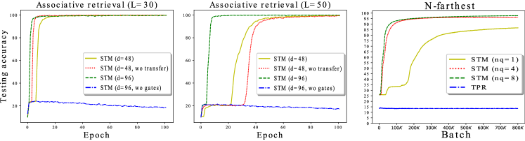
Figure 4: Testing accuracy ($\%$) on associative retrieval L=30 (left), L=50 (middle) and $N^{th}$-farthest (right).

F Implementation of baselines for algorithmic and geometric/graph tasks

Following Graves et al. (2014), we use RMSprop optimizer with a learning rate of $10^{-4}$ and a batch size of 128 for all baselines.

• LSTM and ALSTM: Both use $512$-dimensional hidden vectors for all tasks.

• NTM, DNC: Both use a $256$-dimensional LSTM controller for all tasks. For algorithmic tasks, NTM uses a $128$-slot external memory, each slot is a $32$-dimensional vector. Following the standard setting, NTM uses 1 control head for Copy, RAR and 5 control heads for Priority sort. For geometric/graph tasks, DNC is equipped with $64$-dimensional $20$-slot external memory and $4$-head controller. In geometric/graph problems, $20$ slots are about the number of points/nodes. We also tested with layer-normalized DNC without temporal link matrix and got similar results.

• RMC: We use the default setting with total 1024 dimensions for memory of 8 heads and 8 slots. We also tried with different numbers of slots $\left\{1,4,16\right\}$ and Adam optimizer but the performance did not change.

• STM: We use the same setting across tasks $n_{q}=8$, $d=96$, $n_{r}=96$. $\alpha_{1}$,$\alpha_{2}$, and $\alpha_{3}$ are learnable.

G Order of relationship

In this paper, we do not formally define the concept of order of relationship. Rather, we describe it using concrete examples. When a problem requires to compute the relationship between items, we regard it as a first-order relational problem. For example, sorting is first-order relational. Copy is even zero-order relational since it can be solved without considering item relationships. When a problem requires to compute the relationship between relationships of items, we regard it as a second-order relational problem and so on.

From this observation, we hypothesize that the computational complexity of a problem roughly corresponds to the order of relationship in the problem. For example, if a problem requires a solution whose computational complexity between $O\left(N\right)$ and $O\left(N^{2}\right)$ where $N$ is the input size, it means the solution basically computes the relationship between any pair of input items and thus corresponds to first-order relationship. Table 7 summarizes our hypothesis on the order of relationship in some of our problems.

By design, our proposed STM stores a mixture of relationships between items in a relational memory, which approximately corresponds to a maximum of second-order relational capacity. The distillation process in STM transforms the relational memory to the output and thus determines the order of relationship that STM can offer. We can measure the degree that STM involves in relational mining by analyzing the learned weight $\mathcal{G}_{2}$ of the distillation process. Intuitively, a high-rank transformation $\mathcal{G}_{2}$ can capture more relational information from the relational memory. Trivial low-rank $\mathcal{G}$ corresponds to item-based retrieval without much relational mining (Prop. 5). The numerical rank of a matrix $A$ is defined as $r\left(A\right)=\left\|A\right\|_{F}^{2}/\left\|A\right\|_{2}^{2}$, which relaxes the exact notion of rank (Rudelson & Vershynin, 2007).

We report the numerical rank of learned $\mathcal{G}_{2}\in\mathbb{R}^{6144\times 96}$ for different tasks in Table 8. For each task, we run the training 5 times and take the mean and std. of $r\left(\mathcal{G}_{2}\right)$. The rank is generally higher for tasks that have higher orders of relationship. That said, the model tends to overuse its relational capacity. Even for the zero-order Copy task, the rank for the distillation transformation is still very high.

Task	General complexity	Order
Copy/Associative retrieval	$O\left(N\right)$	0
Sort	$O\left(N\log N\right)$	1
Convex hull	$O\left(N\log N\right)$	1
Shortest path	$O\left(E\log V\right)$	1
Minimum spanning tree	$O\left(E\log V\right)$	1
RAR/$N^{th}$-Farthest	$O\left(N^{2}\log N\right)$	2
Traveling salesman problem	NP-hard	many

Table 7: Order of relationship in some problems.

Task	$r\left(\mathcal{G}_{2}\right)$
Associative retrieval	9.42$\pm$0.5
$N^{th}$-Farthest	83.20$\pm$0.2
Copy	79.00$\pm$0.3
Sort	79.58$\pm$0.1
RAR	83.30$\pm$0.2
Convex hull	80.78$\pm$0.6
Traveling salesman problem	83.58$\pm$0.3
Shortest path	79.81$\pm$0.2
Minimum spanning tree	79.57$\pm$0.5

Table 8: Mean and std. of numerical rank of the leanred weight $\mathcal{G}_{2}$ for several tasks. The upper bound for the rank is 96.

H Geometry and graph task description

In this testbed, we use RMSprop optimizer with a learning rate of $10^{-4}$ and a batch size of 128 for all baselines. STM uses the same setting across tasks $n_{q}=8$, $d=96$, $n_{r}=96$. The random one-hot features can be extended to binary features, which is much harder and will be investigated in our future works.

Convex hull

Given a set of $N$ points with 2D coordinates, the model is trained to output a list of points that forms a convex hull sorted by coordinates. Training is done with $N\sim\left[5,20\right]$. Testing is done with $N=5$ and $N=10$ (no prebuilt dataset available for $N=20$). The output is a sequence of 20-dimensional one-hot vectors representing the features of the solution points in the convex-hull.

Traveling salesman problem

Given a set of $N$ points with 2D coordinates, the model is trained to output a list of points that forms a closed tour sorted by coordinates. Training is done with $N\sim\left[5,10\right]$. Testing is done with $N=5$ and $N=10$. The output is a sequence of 20-dimensional one-hot vectors representing the features of the solution points in the optimal tour.

Shortest path

The graph is generated according to the following rules: (1) choose the number of nodes $N\sim\left[5,20\right]$, (2) after constructing a path that goes through every node in the graph (to make the graph connected), determine randomly the edge between nodes (number of edges $E\sim\left[6,30\right]$), (3) for each edge set the weight $w\sim\left[1,10\right]$. We generate 100,000 and 10,000 graphs for training and testing, respectively. The representation for an input graph is a sequence of triplets followed by 2 feature vectors representing the source and destination node. The output is a sequence of 40-dimensional one-hot feature vectors representing the solution nodes in the shortest path.

Minimum spanning tree

We use the same generated input graphs from the Shortest path task. The representation for an input graph is only a sequence of triplets. The output is a sequence of 40-dimensional one-hot feature vectors representing the features of the nodes in the solution edges of the minimum spanning tree.

Some generated samples of the four tasks are visualized in Fig. 5. Learning curves are given in Fig. 6.

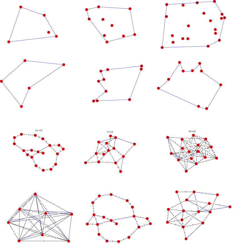
Figure 5: Samples of geometry and graph tasks. From top to bottom: Convex hull, TSP, Shortest path and Minimum spanning tree. Blue denotes the ground-truth solution.

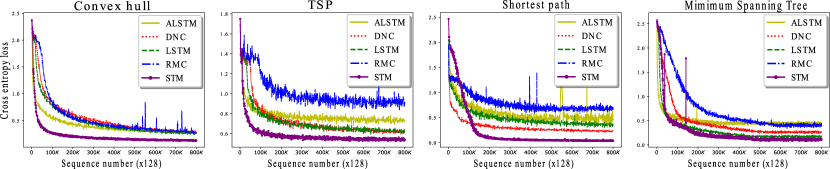
Figure 6: Learning curves on geometry and graph tasks.

I Reinforcement learning task description

We trained Openai Gym’s PongNoFrameskip-v4 using Asynchronous Advantage Actor-Critic (A3C) with hyper-parameters: 32 workers, shared Adam optimizer with a learning rate of $10^{-4}$, $\gamma=0.99$. To extract scene features for LSTM and STM, we use 4 convolutional layers (32 kernels with $5\times 5$ kernel sizes and a stride of 1), each of which is followed by a $2\times 2$ max-pooling layer, resulting in 1024-dimensional feature vectors. The LSTM ’s hidden size is 512. STM uses $n_{q}=8$, $d=96$, $n_{r}=96$.

J bAbI task description

We use the train/validation/test split introduced in bAbI’s en-valid-10k v1.2 dataset. To make STM suitable for question answering task, each story is preprocessed into a sentence-level sequence, which is fed into our STM as the input sequence. The question, which is only 1 sentence, is preprocessed to a query vector. Then, we utilize the Inference module, which takes the query as input to extract the output answer from our relational memory $\mathcal{M}^{r}$. The preprocessing and the Inference module are the same as in Schlag & Schmidhuber (2018). STM’s hyper-parameters are fixed to $n_{q}=20$, $d=90$, $n_{r}=96$. We train our model jointly for 20 tasks with a batch size of $128$, using Adam optimizer with a learning rate of $0.006$, $\beta_{1}=0.9$ and $\beta_{2}=0.99$. Details of all runs are listed in Table 9.

Task	run-1	run-2	run-3	run-4	run-5	run-6	run-7	run-8	run-9	run-10	Mean
1	0.0	0.0	0.0	0.0	0.0	0.0	0.0	0.0	0.0	0.0	0.00 $\pm$ 0.00
2	0.1	0.6	0.1	0.1	0.7	0.2	0.2	0.0	0.1	0.0	0.21 $\pm$ 0.23
3	3.4	3.2	1.0	1.3	2.4	3.8	3.2	0.5	0.9	1.6	2.13 $\pm$ 1.14
4	0.0	0.0	0.0	0.0	0.0	0.0	0.0	0.0	0.0	0.0	0.00 $\pm$ 0.00
5	0.6	0.2	0.6	0.6	0.7	0.5	0.9	0.5	0.7	0.4	0.57 $\pm$ 0.18
6	0.0	0.0	0.0	0.0	0.0	0.1	0.0	0.0	0.0	0.0	0.00 $\pm$ 0.00
7	1.0	0.9	0.5	0.6	0.9	1.4	1.0	0.6	0.5	0.7	0.81 $\pm$ 0.27
8	0.2	0.1	0.1	0.2	0.0	0.0	0.1	0.2	0.1	0.2	0.12 $\pm$ 0.07
9	0.0	0.0	0.0	0.0	0.0	0.0	0.0	0.0	0.0	0.0	0.00 $\pm$ 0.00
10	0.0	0.1	0.0	0.2	0.0	0.0	0.0	0.0	0.0	0.0	0.03 $\pm$ 0.06
11	0.0	0.0	0.1	0.0	0.0	0.0	0.0	0.0	0.0	0.0	0.01 $\pm$ 0.03
12	0.1	0.1	0.1	0.0	0.0	0.1	0.0	0.0	0.0	0.0	0.04 $\pm$ 0.05
13	0.1	0.0	0.0	0.0	0.0	0.0	0.0	0.0	0.0	0.0	0.01 $\pm$ 0.03
14	0.1	0.0	0.1	0.0	0.1	0.3	0.0	0.1	0.5	0.4	0.16 $\pm$ 0.17
15	0.0	0.0	0.0	0.0	0.0	0.0	0.0	0.0	0.0	0.0	0.00 $\pm$ 0.00
16	0.3	0.2	0.2	0.3	0.1	0.3	0.6	0.5	0.3	0.1	0.29 $\pm$ 0.15
17	0.6	2.6	0.4	0.4	0.5	2.1	3.5	0.5	0.9	0.3	1.18 $\pm$ 1.07
18	1.0	0.3	0.2	0.1	0.4	0.4	0.2	0.0	0.1	0.0	0.27 $\pm$ 0.28
19	4.4	0.3	0.8	0.0	8.8	0.4	0.3	0.1	4.7	0.8	2.06 $\pm$ 2.79
20	0.0	0.0	0.0	0.0	0.0	0.5	0.0	0.0	0.0	0.0	0.00 $\pm$ 0.00
Average	0.59	0.43	0.21	0.19	0.73	0.48	0.50	0.15	0.44	0.23	0.39 $\pm$ 0.18
Failed task	0	0	0	0	1	0	0	0	0	0	0.10 $\pm$ 0.30
(>5%)

Table 9: Results from 10 runs of STM on bAbI 10k. Bold denotes best run.

K Characteristics of memory-based neural networks

Table 10 compares the characteristics of common neural networks with memory. Biological plausibility is determined based on the design of the model. It is unlikely that human memory employs RAM-like behaviors as in NTM, DNC, and RMC. Fixed-size memory is inevitable for online and life-long learning, which also reflects biological plausibility. Relational extraction and recurrent dynamics are often required in powerful models. As shown in the table, our proposed model exhibits all the nice features that a memory model should have.

Model	Fixed-size	Relational	Recurrent	Biologically
	memory	extraction	dynamics	plausible
RNN, LSTM	$\checked$	$\vartimes$	$\checked$	$\checked$
NTM, DNC	$\checked$	$\vartimes$	$\checked$	$\vartimes$
RMC	$\checked$	$\checked$	$\checked$	$\vartimes$
Transformer	$\vartimes$	$\checked$	$\vartimes$	$\vartimes$
UT	$\vartimes$	$\checked$	$\checked$	$\vartimes$
Attentional LSTM	$\vartimes$	$\checked$	$\checked$	$\vartimes$
STM	$\checked$	$\checked$	$\checked$	$\checked$

Table 10: Characteristics of some neural memory models

References

- Ba et al. (2016a) Ba, J., Hinton, G. E., Mnih, V., Leibo, J. Z., and Ionescu, C. Using fast weights to attend to the recent past. In Advances in Neural Information Processing Systems, pp. 4331–4339, 2016a.
- Ba et al. (2016b) Ba, J. L., Kiros, J. R., and Hinton, G. E. Layer normalization. arXiv preprint arXiv:1607.06450, 2016b.
- Bahdanau et al. (2014) Bahdanau, D., Cho, K., and Bengio, Y. Neural machine translation by jointly learning to align and translate. arXiv preprint arXiv:1409.0473, 2014.
- Bahdanau et al. (2015) Bahdanau, D., Cho, K., and Bengio, Y. Neural machine translation by jointly learning to align and translate. Proceedings of the International Conference on Learning Representations, 2015.
- Bakker (2002) Bakker, B. Reinforcement learning with long short-term memory. In Advances in neural information processing systems, pp. 1475–1482, 2002.
- Buckley (2005) Buckley, M. J. The role of the perirhinal cortex and hippocampus in learning, memory, and perception. The Quarterly Journal of Experimental Psychology Section B, 58(3-4):246–268, 2005.
- Cohen et al. (1997) Cohen, N. J., Poldrack, R. A., and Eichenbaum, H. Memory for items and memory for relations in the procedural/declarative memory framework. Memory, 5(1-2):131–178, 1997.
- Dehghani et al. (2018) Dehghani, M., Gouws, S., Vinyals, O., Uszkoreit, J., and Kaiser, Ł. Universal transformers. arXiv preprint arXiv:1807.03819, 2018.
- Eichenbaum (1993) Eichenbaum, H. Memory, amnesia, and the hippocampal system. MIT press, 1993.
- Elman (1990) Elman, J. L. Finding structure in time. Cognitive science, 14(2):179–211, 1990.
- Graves et al. (2014) Graves, A., Wayne, G., and Danihelka, I. Neural turing machines. arXiv preprint arXiv:1410.5401, 2014.
- Graves et al. (2016) Graves, A., Wayne, G., Reynolds, M., Harley, T., Danihelka, I., Grabska-Barwińska, A., Colmenarejo, S. G., Grefenstette, E., Ramalho, T., Agapiou, J., et al. Hybrid computing using a neural network with dynamic external memory. Nature, 538(7626):471–476, 2016.
- Henaff et al. (2016) Henaff, M., Weston, J., Szlam, A., Bordes, A., and LeCun, Y. Tracking the world state with recurrent entity networks. arXiv preprint arXiv:1612.03969, 2016.
- Hochreiter & Schmidhuber (1997) Hochreiter, S. and Schmidhuber, J. Long short-term memory. Neural computation, 9(8):1735–1780, 1997.
- Hopfield (1982) Hopfield, J. J. Neural networks and physical systems with emergent collective computational abilities. Proceedings of the national academy of sciences, 79(8):2554–2558, 1982.
- Kim et al. (2018) Kim, J.-H., Jun, J., and Zhang, B.-T. Bilinear attention networks. In Advances in Neural Information Processing Systems, pp. 1564–1574, 2018.
- Kohonen (1972) Kohonen, T. Correlation matrix memories. IEEE transactions on computers, 100(4):353–359, 1972.
- Konkel & Cohen (2009) Konkel, A. and Cohen, N. J. Relational memory and the hippocampus: representations and methods. Frontiers in neuroscience, 3:23, 2009.
- Kumaran & McClelland (2012) Kumaran, D. and McClelland, J. L. Generalization through the recurrent interaction of episodic memories: a model of the hippocampal system. Psychological review, 119(3):573, 2012.
- Le et al. (2018a) Le, H., Tran, T., Nguyen, T., and Venkatesh, S. Variational memory encoder-decoder. In Advances in Neural Information Processing Systems, pp. 1508–1518, 2018a.
- Le et al. (2018b) Le, H., Tran, T., and Venkatesh, S. Dual memory neural computer for asynchronous two-view sequential learning. In Proceedings of the 24th ACM SIGKDD International Conference on Knowledge Discovery; Data Mining, KDD ’18, pp. 1637–1645, New York, NY, USA, 2018b. ACM. ISBN 978-1-4503-5552-0. doi: 10.1145/3219819.3219981. URL http://doi.acm.org/10.1145/3219819.3219981.
- Le et al. (2019) Le, H., Tran, T., and Venkatesh, S. Learning to remember more with less memorization. In International Conference on Learning Representations, 2019. URL https://openreview.net/forum?id=r1xlvi0qYm.
- Le et al. (2020) Le, H., Tran, T., and Venkatesh, S. Neural stored-program memory. In International Conference on Learning Representations, 2020. URL https://openreview.net/forum?id=rkxxA24FDr.
- Marr & Thach (1991) Marr, D. and Thach, W. T. A theory of cerebellar cortex. In From the Retina to the Neocortex, pp. 11–50. Springer, 1991.
- Mnih et al. (2016) Mnih, V., Badia, A. P., Mirza, M., Graves, A., Lillicrap, T., Harley, T., Silver, D., and Kavukcuoglu, K. Asynchronous methods for deep reinforcement learning. In International conference on machine learning, pp. 1928–1937, 2016.
- Munkhdalai et al. (2019) Munkhdalai, T., Sordoni, A., Wang, T., and Trischler, A. Metalearned neural memory. In Advances in Neural Information Processing Systems, pp. 13310–13321, 2019.
- Olson et al. (2006) Olson, I. R., Page, K., Moore, K. S., Chatterjee, A., and Verfaellie, M. Working memory for conjunctions relies on the medial temporal lobe. Journal of Neuroscience, 26(17):4596–4601, 2006.
- Pham & Pagh (2013) Pham, N. and Pagh, R. Fast and scalable polynomial kernels via explicit feature maps. In Proceedings of the 19th ACM SIGKDD international conference on Knowledge discovery and data mining, pp. 239–247. ACM, 2013.
- Rojas (2013) Rojas, R. Neural networks: a systematic introduction. Springer Science & Business Media, 2013.
- Rudelson & Vershynin (2007) Rudelson, M. and Vershynin, R. Sampling from large matrices: An approach through geometric functional analysis. Journal of the ACM (JACM), 54(4):21, 2007.
- Santoro et al. (2017) Santoro, A., Raposo, D., Barrett, D. G., Malinowski, M., Pascanu, R., Battaglia, P., and Lillicrap, T. A simple neural network module for relational reasoning. In Advances in neural information processing systems, pp. 4967–4976, 2017.
- Santoro et al. (2018) Santoro, A., Faulkner, R., Raposo, D., Rae, J., Chrzanowski, M., Weber, T., Wierstra, D., Vinyals, O., Pascanu, R., and Lillicrap, T. Relational recurrent neural networks. In Advances in Neural Information Processing Systems, pp. 7299–7310, 2018.
- Schlag & Schmidhuber (2017) Schlag, I. and Schmidhuber, J. Gated fast weights for on-the-fly neural program generation. In NIPS Metalearning Workshop, 2017.
- Schlag & Schmidhuber (2018) Schlag, I. and Schmidhuber, J. Learning to reason with third order tensor products. In Advances in Neural Information Processing Systems, pp. 9981–9993, 2018.
- Smolensky (1990) Smolensky, P. Tensor product variable binding and the representation of symbolic structures in connectionist systems. Artificial intelligence, 46(1-2):159–216, 1990.
- Tenenbaum & Freeman (2000) Tenenbaum, J. B. and Freeman, W. T. Separating style and content with bilinear models. Neural computation, 12(6):1247–1283, 2000.
- Vaswani et al. (2017) Vaswani, A., Shazeer, N., Parmar, N., Uszkoreit, J., Jones, L., Gomez, A. N., Kaiser, Ł., and Polosukhin, I. Attention is all you need. In Advances in neural information processing systems, pp. 5998–6008, 2017.
- Vinyals et al. (2015) Vinyals, O., Fortunato, M., and Jaitly, N. Pointer networks. In Advances in Neural Information Processing Systems, pp. 2692–2700, 2015.
- von der Malsburg (1981) von der Malsburg, C. The correlation theory of brain function, 1981. URL http://cogprints.org/1380/.
- Weston et al. (2015) Weston, J., Bordes, A., Chopra, S., Rush, A. M., van Merriënboer, B., Joulin, A., and Mikolov, T. Towards ai-complete question answering: A set of prerequisite toy tasks. arXiv preprint arXiv:1502.05698, 2015.
- Yu et al. (2017) Yu, Z., Yu, J., Fan, J., and Tao, D. Multi-modal factorized bilinear pooling with co-attention learning for visual question answering. In Proceedings of the IEEE international conference on computer vision, pp. 1821–1830, 2017.
- Zeithamova et al. (2012) Zeithamova, D., Schlichting, M. L., and Preston, A. R. The hippocampus and inferential reasoning: building memories to navigate future decisions. Frontiers in human neuroscience, 6:70, 2012.
- Zhang & Zhou (2017) Zhang, W. and Zhou, B. Learning to update auto-associative memory in recurrent neural networks for improving sequence memorization. ArXiv, abs/1709.06493, 2017.