Random Smoothing Might be Unable to Certify $\ell_{\infty}$ Robustness for High-Dimensional Images

Abstract

We show a hardness result for random smoothing to achieve certified adversarial robustness against attacks in the $\ell_{p}$ ball of radius $\epsilon$ when $p>2$. Although random smoothing has been well understood for the $\ell_{2}$ case using the Gaussian distribution, much remains unknown concerning the existence of a noise distribution that works for the case of $p>2$. This has been posed as an open problem by Cohen et al. (2019) and includes many significant paradigms such as the $\ell_{\infty}$ threat model. In this work, we show that any noise distribution $\mathcal{D}$ over $\mathbb{R}^{d}$ that provides $\ell_{p}$ robustness for all base classifiers with $p>2$ must satisfy $\operatorname*{\mathbb{E}}\eta_{i}^{2}=\Omega(d^{1-2/p}\epsilon^{2}(1-\delta)/\delta^{2})$ for 99% of the features (pixels) of vector $\eta\sim\mathcal{D}$, where $\epsilon$ is the robust radius and $\delta$ is the score gap between the highest-scored class and the runner-up. Therefore, for high-dimensional images with pixel values bounded in $[0,255]$, the required noise will eventually dominate the useful information in the images, leading to trivial smoothed classifiers.

1 Introduction

Adversarial robustness has been a critical object of study in various fields, including machine learning (Zhang et al., 2019; Madry et al., 2017), computer vision (Szegedy et al., 2013; Yang et al., 2019), and many other domains (Lecuyer et al., 2019). In machine learning and computer vision, the study of adversarial robustness has led to significant advances in defending against attacks in the form of perturbed input images, where the data is high dimensional but each feature is bounded in $[0,255]$. The problem can be stated as that of learning a non-trivial classifier with high test accuracy on the adversarial images. The adversarial perturbation is either restricted to be in an $\ell_{p}$ ball of radius $\epsilon$ centered at $0$, or is measured under other threat models such as Wasserstein distance and adversarial rotation (Wong et al., 2019; Brown et al., 2018). The focus of this work is the former setting.

Despite a large amount of work on adversarial robustness, many fundamental problems remain open. One of the challenges is to end the long-standing arms race between adversarial defenders and attackers: defenders design empirically robust algorithms which are later exploited by new attacks designed to undermine those defenses (Athalye et al., 2018). This motivate the study of certified robustness (Raghunathan et al., 2018; Wong et al., 2018)—algorithms that are provably robust to the worst-case attacks—among which random smoothing (Cohen et al., 2019; Li et al., 2019; Lecuyer et al., 2019) has received significant attention in recent years. Algorithmically, random smoothing takes a base classifier $f$ as an input, and outputs a smooth classifier $g$ by repeatedly adding i.i.d. noises to the input examples and outputting the most-likely class. Random smoothing has many appealing properties that one could exploit: it is agnostic to network architecture, is scalable to deep networks, and perhaps most importantly, achieves state-of-the-art certified $\ell_{2}$ robustness for deep learning based classifiers (Cohen et al., 2019; Li et al., 2019; Lecuyer et al., 2019).

Open problems in random smoothing. Given the rotation invariance of Gaussian distribution, most positive results for random smoothing have focused on the $\ell_{2}$ robustness achieved by smoothing with the Gaussian distribution (see Theorem 2.1). However, the existence of a noise distribution for general $\ell_{p}$ robustness has been posed as an open question by Cohen et al. (2019):

We suspect that smoothing with other noise distributions may lead to similarly natural robustness guarantees for other perturbation sets such as general $\ell_{p}$ norm balls.

Several special cases of the conjecture have been proven for $p<2$. Li et al. (2019) show that $\ell_{1}$ robustness can be achieved with the Laplacian distribution, and Lee et al. (2019) show that $\ell_{0}$ robustness can be achieved with a discrete distribution. Much remains unknown concerning the case when $p>2$. On the other hand, the most standard threat model for adversarial examples is $\ell_{\infty}$ robustness, among which 8-pixel and 16-pixel attacks have received significant attention in the computer vision community (i.e., the adversary can change every pixel by 8 or 16 intensity values, respectively). In this paper, we derive lower bounds on the magnitude of noise required for certifying $\ell_{p}$ robustness that highlights a phase transition at $p=2$. In particular, for $p>2$, the noise that must be added to each feature of the input examples grows with the dimension $d$ in expectation, while it can be constant for $p\leq 2$.

Preliminaries. Given a base classifier $f:\mathbb{R}^{d}\rightarrow\mathcal{Y}$ and smoothing distribution $\mathcal{D}$, the randomly smoothed classifier is defined as follows: for each class $y\in\mathcal{Y}$, define the score of class $y$ at point $x$ to be $G_{y}(x;\mathcal{D},f)=\operatorname*{Pr}_{\eta\sim\mathcal{D}}(f(x+\eta)=y)$. Then the smoothed classifier outputs the class with the highest score: $g(x;\mathcal{D},f)=\operatorname*{argmax}_{y}G_{y}(x;\mathcal{D},f)$.

The key property of smoothed classifiers is that the scores $G_{y}(x;\mathcal{D},f)$ change slowly as a function of the input point $x$ (the rate of change depends on $\mathcal{D}$). It follows that if there is a gap between the highest and second highest class scores at a point $x$, the smoothed classifier $g(\cdot;\mathcal{D},f)$ must be constant in a neighborhood of $x$. We denote the score gap by $\Delta(x;\mathcal{D},f)=G_{a}(x;\mathcal{D},f)-G_{b}(x;\mathcal{D},f)$, where $a=\operatorname*{argmax}_{y}G_{y}(x;\mathcal{D},f)$ and $b=\operatorname*{argmax}_{y\neq a}G_{y}(x;\mathcal{D},f)$.

Definition 1 ($(\mathcal{A},\delta)$- and $(\epsilon,\delta)$-robustness).

For any set $\mathcal{A}\subseteq\mathbb{R}^{d}$ and $\delta\in[0,1]$, we say that the smoothed classifier $g$ is $(\mathcal{A},\delta)$-robust if for all $x\in\mathbb{R}^{d}$ with $\Delta(x;\mathcal{D},f)>\delta$, we have that $g(x+v;\mathcal{D},f)=g(x;\mathcal{D},f)$ for all $v\in\mathcal{A}$. For a given norm $\left\|\cdot\right\|$, we also say that $g$ is $(\epsilon,\delta)$-robust with respect to $\left\|\cdot\right\|$ if it is $(\mathcal{A},\delta)$-robust with $\mathcal{A}=\{v\in\mathbb{R}^{d}:\left\|v\right\|\leq\epsilon\}$.

When the base classifier $f$ and the smoothing distribution $\mathcal{D}$ are clear from context, we will simply write $G_{y}(x)$, $g(x)$, and $\Delta(x)$. We often refer to a sample from the distribution $\mathcal{D}$ as noise, and use noise magnitude to refer to squared $\ell_{2}$ norm of a noise sample. Finally, we use $\mathcal{D}+v$ to denote the distribution of $\eta+v$, where $\eta\sim\mathcal{D}$.

1.1 Our results

Our main results derive lower bounds on the magnitude of noise sampled from any distribution $\mathcal{D}$ that leads to $(\epsilon,\delta)$-robustness with respect to $\left\|\cdot\right\|_{p}$ for all possible base classifiers $f:\mathbb{R}^{d}\to\mathcal{Y}$. A major strength of random smoothing is that it provides certifiable robustness guarantees without making any assumption on the base classifier $f:\mathbb{R}^{d}\to\mathcal{Y}$. For example, the results of Cohen et al. (2019) imply that using a Gaussian smoothing distribution with standard deviation $\sigma=\frac{2\epsilon}{\delta}$ guarantees that $g(\cdot;\mathcal{D},f)$ is $(\epsilon,\delta)$-robust with respect to $\left\|\cdot\right\|_{2}$ for every possible base classifier $f:\mathbb{R}^{d}\to\mathcal{Y}$. We show that there is a phase transition at $p=2$, and that ensuring $(\epsilon,\delta)$-robustness for all base classifiers $f$ with respect to $\ell_{p}$ norms with $p>2$ requires that the noise magnitude grows non-trivially with the dimension $d$ of the input space. In particular, for image classification tasks where the data is high dimensional and each feature is bounded in the range $[0,255]$, this implies that for sufficiently large dimensions, the necessary noise will dominate the signal in each example.

The following result, proved in Appendix A, shows that any distribution $\mathcal{D}$ that provides $(\mathcal{A},\delta)$-robustness for every possible base classifier $f:\mathbb{R}^{d}\to\mathcal{Y}$ must be approximately translation-invariant to all translations $v\in\mathcal{A}$. More formally, for every $v\in\mathcal{A}$, we must have that the total variation distance between $\mathcal{D}$ and $\mathcal{D}+v$, denoted by $\operatorname{TV}(\mathcal{D},\mathcal{D}+v)$, is bounded by $\delta$. The rest of our results will be consequences of this approximate translation-invariance property. lemmalemRobustToTV Let $\mathcal{D}$ be a distribution on $\mathbb{R}^{d}$ such that for every (randomized) classifier $f:\mathbb{R}^{d}\to\mathcal{Y}$, the smoothed classifier $g(\cdot;\mathcal{D},f)$ is $(\mathcal{A},\delta)$-robust. Then for all $v\in\mathcal{A}$, we have $\operatorname{TV}(\mathcal{D},\mathcal{D}+v)\leq\delta$.

Lower bound on noise magnitude.

Our first result is a lower bound on the expected squared $\ell_{2}$-magnitude of a sample $\eta\sim\mathcal{D}$ for any distribution $\mathcal{D}$ that is approximately invariant to $\ell_{p}$-translations of size $\epsilon$.

theoremthmLowerBound Fix any $p\geq 2$ and let $\mathcal{D}$ be a distribution on $\mathbb{R}^{d}$ such that there exists a radius $\epsilon$ and total variation bound $\delta$ satisfying that for all $v\in\mathbb{R}^{d}$ with $\left\|v\right\|_{p}\leq\epsilon$ we have $\operatorname{TV}(\mathcal{D},\mathcal{D}+v)\leq\delta$. Then

$$\operatorname*{\mathbb{E}}_{\eta\sim\mathcal{D}}\left\|\eta\right\|_{2}^{2}\geq\frac{\epsilon^{2}d^{2-2/p}}{800}\cdot\frac{1-\delta}{\delta^{2}}.$$

As a consequence of Section 1.1 and Lemma 1.1, it follows that any distribution that ensures $(\epsilon,\delta)$-robustness with respect to $\left\|\cdot\right\|_{p}$ for any base classifier $f$ must also satisfy the same lower bound.

Phase transition at $p=2$.

The lower bound given by Section 1.1 implies a phase transition in the nature of distributions $\mathcal{D}$ that are able to ensure $(\epsilon,\delta)$-robustness with respect to $\left\|\cdot\right\|_{p}$ that occurs at $p=2$. For $p\leq 2$, the necessary expected squared $\ell_{2}$-magnitude of a sample from $\mathcal{D}$ grows only like $\sqrt{d}$, which is consistent with adding a constant level of noise to every feature in the input example (e.g., as would happen when using a Gaussian distribution with standard deviation $\sigma=\frac{2\epsilon}{\delta}$). On the other hand, for $p>2$, the expected $\ell_{2}$ magnitude of a sample from $\mathcal{D}$ grows strictly faster than $\sqrt{d}$, which, intuitively, requires that the noise added to each component of the input example must scale with the input dimension $d$, rather than remaining constant as in the $p\leq 2$ regime. More formally, we prove the following:

[hardness of random smoothing]theoremthmComponentProperties Fix any $p>2$ and let $\mathcal{D}$ be a distribution on $\mathbb{R}^{d}$ such that for every (randomized) classifier $f:\mathbb{R}^{d}\to\mathcal{Y}$, the smoothed classifier $g(\cdot;\mathcal{D},f)$ is $(\mathcal{A},\delta)$-robust. Let $\eta$ be a sample from $\mathcal{D}$. Then at least 99% of the components of $\eta$ satisfy $\operatorname*{\mathbb{E}}\eta_{i}^{2}=\Omega(\frac{\epsilon^{2}d^{1-2/p}(1-\delta)}{\delta^{2}})$. Moreover, if $\mathcal{D}$ is a product measure of i.i.d. noise (i.e., $\mathcal{D}=(\mathcal{D}^{\prime})^{d}$), then the tail of $\mathcal{D}^{\prime}$ satisfies $\operatorname*{Pr}_{\zeta\sim\mathcal{D}^{\prime}}(|\zeta|>s)\geq\left(\frac{c\epsilon(1-\delta)}{s\delta}\right)^{2p/(p-2)}$ for some $s>c\epsilon(1-\delta)/\delta$, where $c$ is an absolute constant. In other words, $\mathcal{D}^{\prime}$ is a heavy-tailed distribution.

The phase transition at $p=2$ is more clearly evident from Section 1.1. In particular, the variance of most components of the noise must grow with $d^{1-2/p}$. Section 1.1 shows that any distribution that provides $(\epsilon,\delta)$-robustness with respect to $\left\|\cdot\right\|_{p}$ for $p>2$ must have very high variance in most of its component distributions when the dimension $d$ is large. In particular, for $p=\infty$ the variance grows linearly with the dimension. Similarly, if we use a product distribution to achieve $(\epsilon,\delta)$-robustness with respect to $\left\|\cdot\right\|_{p}$ with $p>2$, then each component of the noise distribution must be heavy-tailed and is likely to generate very large perturbations.

1.2 Technical overview

Total-variation bound of noise magnitude. Our results demonstrate a strong connection between the required noise magnitude $\operatorname*{\mathbb{E}}\|\eta\|_{2}^{2}$ in random smoothing and the total variation distance between $\mathcal{D}$ and its shifted distribution $\mathcal{D}+v$ in the worst-case direction $v$. The total variation distance has a very natural explanation on the hardness of testing $\mathcal{D}$ v.s. $\mathcal{D}+v$: any classifier cannot distinguish $\mathcal{D}$ from $\mathcal{D}+v$ with a good probability related to $\operatorname{TV}(\mathcal{D},\mathcal{D}+v)$. Our analysis applies the following techniques.

Warm-up: one-dimensional case. We begin our analysis of Theorem 1.1 with the one-dimension case, by studying the projection of noise $\eta\in\mathbb{R}^{d}$ on a direction $v\in\mathbb{R}^{d}$. A simple use of Chebyshev’s inequality implies $\operatorname*{\mathbb{E}}_{\eta\sim\mathcal{D}}|v^{\top}\eta|^{2}\geq\left\|v\right\|^{2}_{4}(1-\delta)/8$. To see this, let $\eta$ be a sample from $\mathcal{D}$ and let $\eta^{\prime}=\eta+v$ so that $\eta^{\prime}$ is a sample from $\mathcal{D}+v$. Define $Z=v^{\top}\eta$ and $Z^{\prime}=v^{\top}\eta^{\prime}=Z+\left\|v\right\|_{2}^{2}$. Define $r=\left\|v\right\|_{2}^{2}/2$ so that the intervals $\mathcal{A}=(-r,r)$ and $\mathcal{B}=[\left\|v\right\|_{2}^{2}-r,\left\|v\right\|_{2}^{2}+r]$ are disjoint. From Chebyshev’s inequality, we have $\operatorname*{Pr}(Z\in\mathcal{A})\geq 1-\operatorname*{\mathbb{E}}|Z|^{2}/r^{2}$. Similarly, $\operatorname*{Pr}(Z^{\prime}\in\mathcal{B})\geq 1-\operatorname*{\mathbb{E}}|Z|^{2}/r^{2}$ and, since $\mathcal{A}$ and $\mathcal{B}$ are disjoint, this implies $\operatorname*{Pr}(Z^{\prime}\in\mathcal{A})<\operatorname*{\mathbb{E}}|Z|^{2}/r^{2}$. Therefore, $\operatorname{TV}(\mathcal{D},\mathcal{D}+v)\geq\operatorname*{Pr}(Z\in\mathcal{A})-\operatorname*{Pr}(Z^{\prime}\in\mathcal{A})\geq 1-2\operatorname*{\mathbb{E}}|Z|^{2}/r^{2}$. The claim follows from rearranging this inequality and the fact $\delta\geq\operatorname{TV}(\mathcal{D},\mathcal{D}+v)$.

The remainder of the one-dimension case is to show $\operatorname*{\mathbb{E}}_{\eta\sim\mathcal{D}}|v^{\top}\eta|\geq\left\|v\right\|^{2}_{2}\frac{(1-\delta)^{2}}{8\delta}$. To this end, we exploit a nice property of total variation distance in $\mathbb{R}$: every $\epsilon$-interval $I=[a,a+\epsilon)$ satisfies $\mathcal{D}(I)\leq\operatorname{TV}(\mathcal{D},\mathcal{D}+\epsilon)$. We note that for any $\tau\geq 0$, rearranging Markov’s inequality gives $\operatorname*{\mathbb{E}}|v^{\top}\eta|\geq\tau\operatorname*{Pr}(|v^{\top}\eta|>\tau)=\tau(1-\operatorname*{Pr}(|v^{\top}\eta|\leq\tau))$. We can cover the set $\{x\in\mathbb{R}\,:\,|x|\leq\tau\}$ using $\lceil\frac{2\tau}{\epsilon}\rceil$ intervals of width $\epsilon=\|v\|_{2}^{2}$ and, by this property, each of those intervals has probability mass at most $\delta$. It follows that $\operatorname*{Pr}(|v^{\top}\eta|\leq\tau)\leq\lceil\frac{2\tau}{\epsilon}\rceil\delta$, implying $\operatorname*{\mathbb{E}}|v^{\top}\eta|\geq\tau(1-\lceil\frac{2\tau}{\epsilon}\rceil\delta)$. Finally, we optimize $\tau$ to obtain the bound $\operatorname*{\mathbb{E}}_{\eta\sim\mathcal{D}}|v^{\top}\eta|\geq\|v\|_{2}^{2}\frac{(1-\delta)^{2}}{8\delta}$, as desired.

Extension to the $d$-dimensional case. A bridge to connect one-dimensional case with $d$-dimensional case is the Pythagorean theorem: if there exists a set of orthogonal directions $v_{i}$’s such that $\operatorname*{\mathbb{E}}_{\eta\sim\mathcal{D}}|v_{i}^{\top}\eta|^{2}\geq\frac{\left\|v_{i}\right\|^{4}_{2}}{200}\frac{1-\delta}{\delta^{2}}$ and $\|v_{i}\|_{2}=\epsilon d^{1/2-1/p}$ (the furthest distance to $x$ in the $\ell_{p}$ ball $\mathcal{B}_{p}(x,\epsilon)$), the Pythagorean theorem implies the result for the $d$-dimensional case straightforwardly. The existence of a set of orthogonal directions that satisfy these requirements is easy to find for the $\ell_{2}$ case, because the $\ell_{2}$ ball is isotropic and any set of orthogonal bases of $\mathbb{R}^{d}$ satisfies the conditions. However, the problem is challenging for the $\ell_{p}$ case, since the $\ell_{p}$ ball is not isotropic in general. In Corollary 3.6, we show that there exist at least $d/2$ $v_{i}$’s which satisfy the requirements. Using the Pythagorean theorem in the subspace spanned by such $v_{i}$’s gives Theorem 1.1.

Peeling argument and tail probability. We now summarize our main techniques to prove Theorem 1.1. By $\|\eta\|_{2}\leq\sqrt{d}\|\eta\|_{\infty}$, Theorem 1.1 implies $\operatorname*{\mathbb{E}}\eta_{i}^{2}\geq\frac{\epsilon d^{1/2-1/p}}{800}\cdot\frac{1-\delta}{\delta^{2}}$ for at least one index $i$, which shows that at least one component of $\eta$ is large. However, this guarantee only highlights the largest pixel of $|\eta|$. Rather than working with the $\ell_{\infty}$-norm of $\eta$, we apply a similar argument to show that the variance of at least one component of $\eta$ must be large. Next, we consider the $(d-1)$-dimensional distribution obtained by removing the highest-variance feature. Applying an identical argument, the highest-variance remaining feature must also be large. Each time we repeat this procedure, the strength of the variance lower bound decreases since the dimensionality of the distribution is decreasing. However, we can apply this peeling strategy for any constant fraction of the components of $\eta$ to obtain lower bounds. The tail-probability guarantee in Theorem 1.1 follows a standard moment analysis in (Vershynin, 2018).

Summary of our techniques. Our proofs—in particular, the use of the Pythagorean theorem—show that defending against adversarial attacks in the $\ell_{p}$ ball of radius $\epsilon$ by random smoothing is almost as hard as defending against attacks in the $\ell_{2}$ ball of radius $\epsilon d^{1/2-1/p}$. Therefore, the $\ell_{\infty}$ certification procedure—firstly using Gaussian smoothing to certify $\ell_{2}$ robustness and then dividing the $\ell_{2}$ certified radius by $\sqrt{d}$ as in (Salman et al., 2019)—is almost an optimal random smoothing approach for certifying $\ell_{\infty}$ robustness. The principle might hold generally for other threat models beyond $\ell_{p}$ robustness, and sheds light on the design of new random smoothing and proofs of hardness in the other threat models broadly.

2 Related Works

$\ell_{2}$ robustness. Probably one of the most well-understood results for random smoothing is the $\ell_{2}$ robustness. With Gaussian random noises, Lecuyer et al. (2019) and Li et al. (2019) provided the first guarantee of random smoothing and was later improved by Cohen et al. (2019) with the following theorem.

Theorem 2.1 (Theorem 1 of Cohen et al. (2019)).

Let $f:\mathbb{R}^{d}\rightarrow\mathcal{Y}$ by any deterministic or random classifier, and let $\eta\sim\mathcal{N}(0,\sigma^{2}I)$. Let $g(x)=\operatorname*{argmax}_{c\in\mathcal{Y}}\Pr(f(x+\eta)=c)$. Suppose $c_{A}\in\mathcal{Y}$ and $\underline{p_{A}},\overline{p_{B}}\in[0,1]$ satisfy: $\Pr(f(x+\eta)=c_{A})\geq\underline{p_{A}}\geq\overline{p_{B}}\geq\max_{c\not=c_{A}}\Pr(f(x+\eta)=c).$ Then $g(x+\delta)=c_{A}$ for all $\|\delta\|_{2}<\epsilon$, where $\epsilon=\frac{\sigma}{2}(\Phi^{-1}(\underline{p_{A}})-\Phi^{-1}(\overline{p_{B}}))$, and $\Phi(\cdot)$ is the cumulative distribution function of standard Gaussian distribution.

Note that Theorem 2.1 holds for arbitrary classifier. Thus a hardness result of random smoothing—the one in an opposite direction of Theorem 2.1—requires finding a hard instance of classifier $f$ such that a similar conclusion of Theorem 2.1 does not hold, i.e., the resulting smoothed classifier $g$ is trivial as the noise variance is too large. Our results of Theorems 1.1 and 1.1 are in such flavour. Beyond the top-$1$ predictions in Theorem 2.1, Jia et al. (2020) studied the certified robustness for top-$k$ predictions via random smoothing under Gaussian noise and derive a tight robustness bound in $\ell_{2}$ norm. In this paper, however, we study the standard setting of top-$1$ predictions.

$\ell_{p}$ robustness. Beyond the $\ell_{2}$ robustness, random smoothing also achieves the state-of-the-art certified $\ell_{p}$ robustness for $p<2$. Lee et al. (2019) provided adversarial robustness guarantees and associated random-smoothing algorithms for the discrete case where the adversary is $\ell_{0}$ bounded. Li et al. (2019) suggested replacing Gaussian with Laplacian noise for the $\ell_{1}$ robustness. Dvijotham et al. (2020) introduced a general framework for proving robustness properties of smoothed classifiers in the black-box setting using $f$-divergence. However, much remains unknown concerning the effectiveness of random smoothing for $\ell_{p}$ robustness with $p>2$. Salman et al. (2019) proposed an algorithm for certifying $\ell_{\infty}$ robustness, by firstly certifying $\ell_{2}$ robustness via the algorithm of Cohen et al. (2019) and then dividing the certified $\ell_{2}$ radius by $\sqrt{d}$. However, the certified $\ell_{\infty}$ radius by this procedure is as small as $\mathcal{O}(1/\sqrt{d})$, in contrast to the constant certified radius as discussed in this paper.

Training algorithms. While random smoothing certifies inference-time robustness for any given base classifier $f$, the certified robust radius might vary a lot for different training methods. This motivates researchers to design new training algorithms of $f$ that particularly adapts to random smoothing. Zhai et al. (2020) trained a robust smoothed classifier via maximizing the certified radius. In contrast to using naturally trained classifier in (Cohen et al., 2019), Salman et al. (2019) combined adversarial training of Madry et al. (2017) with random smoothing in the training procedure of $f$. In our experiment, we introduce a new baseline which combines TRADES (Zhang et al., 2019) with random smoothing to train a robust smoothed classifier.

3 Analysis of Main Results

In this section we prove Section 1.1 and Section 1.1.

3.1 Analysis of Theorem 1.1

In this section we prove Section 1.1. Our proof has two main steps: first, we study the one-dimensional version of the problem and prove two complementary lower bounds on the magnitude of a sample $\eta$ drawn from a distribution $\mathcal{D}$ over $\mathbb{R}$ with the property that for all $v\in\mathbb{R}$ with $|v|\leq\epsilon$ we have $\operatorname{TV}(\mathcal{D},\mathcal{D}+v)\leq\delta$. Next, we show how to apply this argument to $\Omega(d)$ orthogonal 1-dimensional subspaces in $\mathbb{R}^{d}$ to lower bound the expected magnitude of a sample drawn from a distribution $\mathcal{D}$ over $\mathbb{R}^{d}$, with the property that for all $v\in\mathbb{R}^{d}$ with $\left\|v\right\|_{p}\leq\epsilon$, we have $\operatorname{TV}(\mathcal{D},\mathcal{D}+v)\leq\delta$.

One-dimensional results.

Our first result lower bounds the magnitude of a sample from any distribution $\mathcal{D}$ in terms of the total variation distance between $\mathcal{D}$ and $\mathcal{D}+\epsilon$ for any $\epsilon\geq 0$.

Lemma 3.1.

Let $\mathcal{D}$ be any distribution on $\mathbb{R}$, $\eta$ be a sample from $\mathcal{D}$, $\epsilon\geq 0$, and let $\delta=\operatorname{TV}(\mathcal{D},\mathcal{D}+\epsilon)$. Then we have

$$\operatorname*{\mathbb{E}}|\eta|^{2}\geq\frac{\epsilon^{2}}{200}\cdot\frac{1-\delta}{\delta^{2}}.$$

We prove Lemma 3.1 using two complementary lower bounds. The first lower bound is tighter for large $\delta$, while the second lower bound is tighter when $\delta$ is close to zero. Taking the maximum of the two bounds proves Lemma 3.1.

Lemma 3.2.

Let $\mathcal{D}$ be any distribution on $\mathbb{R}$, $\eta$ be a sample from $\mathcal{D}$, $\epsilon\geq 0$, and let $\delta=\operatorname{TV}(\mathcal{D},\mathcal{D}+\epsilon)$. Then we have

$$\operatorname*{\mathbb{E}}|\eta|^{2}\geq\frac{\epsilon^{2}}{8}\cdot(1-\delta).$$

Proof.

Let $\eta^{\prime}=\eta+\epsilon$ so that $\eta^{\prime}$ is a sample from $\mathcal{D}+\epsilon$ and define $r=\epsilon/2$ so that the sets $\mathcal{A}=(-r,r)$ and $\mathcal{B}=[\epsilon-r,\epsilon+r]$ are disjoint. From Chebyshev’s inequality, we have that $\operatorname*{Pr}(\eta\in\mathcal{A})=1-\operatorname*{Pr}(|\eta|\geq r)\geq 1-\frac{\operatorname*{\mathbb{E}}|\eta|^{2}}{r^{2}}$. Further, since $\eta^{\prime}\in\mathcal{B}$ if and only if $\eta\in\mathcal{A}$, we have $\operatorname*{Pr}(\eta^{\prime}\in\mathcal{B})\geq 1-\frac{\operatorname*{\mathbb{E}}|\eta|^{2}}{r^{2}}$. Next, since $\mathcal{A}$ and $\mathcal{B}$ are disjoint, it follows that $\operatorname*{Pr}(\eta^{\prime}\in\mathcal{A})\leq 1-\operatorname*{Pr}(\eta^{\prime}\in\mathcal{B})\leq 1-1+\frac{\operatorname*{\mathbb{E}}|\eta|^{2}}{r^{2}}=\frac{\operatorname*{\mathbb{E}}|\eta|^{2}}{r^{2}}$. Finally, we have $\delta\geq\operatorname*{Pr}(\eta\in\mathcal{A})-\operatorname*{Pr}(\eta^{\prime}\in\mathcal{A})\geq 1-\frac{2\operatorname*{\mathbb{E}}|\eta|^{2}}{r^{2}}=1-\frac{8\operatorname*{\mathbb{E}}|\eta|^{2}}{\epsilon^{2}}$. Rearranging this inequality proves the claim. ∎

Next, we prove a tighter bound when $\delta$ is close to zero. The key insight is that no interval $I\subseteq\mathbb{R}$ of width $\epsilon$ can have probability mass larger than $\operatorname{TV}(\mathcal{D},\mathcal{D}+\epsilon)$. This implies that the mass of $\mathcal{D}$ cannot concentrate too close to the origin, leading to lower bounds on the expected magnitude of a sample from $\mathcal{D}$.

Lemma 3.3.

Let $\mathcal{D}$ be any distribution on $\mathbb{R}$, $\eta$ be a sample from $\mathcal{D}$, $\epsilon\geq 0$, and let $\delta=\operatorname{TV}(\mathcal{D},\mathcal{D}+\epsilon)$. Then we have

$$\operatorname*{\mathbb{E}}|\eta|\geq\frac{\epsilon}{8}\cdot\frac{(1-\delta)^{2}}{\delta},$$

which implies $\operatorname*{\mathbb{E}}|\eta|^{2}\geq\frac{\epsilon^{2}}{64}\cdot\frac{(1-\delta)^{4}}{\delta^{2}}$.

Proof.

The key step in the proof is to show that every interval $\mathcal{I}=[a,a+\epsilon)$ of length $\epsilon$ has probability mass at most $\delta$ under the distribution $\mathcal{D}$. Once we have established this fact, then the proof is as follows: for any $\tau\geq 0$, rearranging Markov’s inequality gives $\operatorname*{\mathbb{E}}|\eta|\geq\tau\operatorname*{Pr}(|\eta|>\tau)=\tau(1-\operatorname*{Pr}(|\eta|\leq\tau))$. We can cover the set $\{x\in\mathbb{R}\,:\,|x|\leq\tau\}$ using $\lceil\frac{2\tau}{\epsilon}\rceil$ intervals of width $\epsilon$ and each of those intervals has probability mass at most $\delta$. It follows that $\operatorname*{Pr}(|\eta|\leq\tau)\leq\lceil\frac{2\tau}{\epsilon}\rceil\delta$, implying $\operatorname*{\mathbb{E}}|\eta|\geq\tau(1-\lceil\frac{2\tau}{\epsilon}\rceil\delta)$. Since $\lceil\frac{2\tau}{\epsilon}\rceil\leq\frac{2\tau}{\epsilon}+1$, we have $\operatorname*{\mathbb{E}}|\eta|\geq(1-\delta)\tau-\frac{2\delta}{\epsilon}\tau^{2}$. Finally, we optimize $\tau$ to get the strongest bound. The strongest bound is obtained at $\tau=\frac{\epsilon(1-\delta)}{4\delta}$, which gives $\operatorname*{\mathbb{E}}|\eta|\geq\frac{\epsilon(1-\delta)^{2}}{8\delta}$.

It remains to prove the claim that all intervals of length $\epsilon$ have probability mass at most $\delta$. Let $\mathcal{I}=[a,a+\epsilon)$ be any such interval. The proof has two steps: first, we partition $\mathbb{R}$ using a collection of translated copies of the interval $\mathcal{I}$, and show that the difference in probability mass between any pair of intervals in the partition is at most $\delta$. Then, given that there must be intervals with probability mass arbitrarily close to zero, this implies that the probability mass of any interval (and in particular, the probability mass of $\mathcal{I}$) is upper bounded by $\delta$.

For each integer $i\in\mathbb{Z}$, let $\mathcal{I}_{i}=\mathcal{I}+i\epsilon=\{x+i\epsilon:x\in\mathcal{I}\}$ be a copy of the interval $\mathcal{I}$ translated by $i\epsilon$. By construction the set of intervals $\mathcal{I}_{i}$ for $i\in\mathbb{Z}$ forms a partition of $\mathbb{R}$. For any indices $i<j$, we can express the difference in probability mass between $\mathcal{I}_{i}$ and $\mathcal{I}_{j}$ as a telescoping sum: $\mathcal{D}(\mathcal{I}_{j})-\mathcal{D}(\mathcal{I}_{i})=\sum_{k=i}^{j-1}[\mathcal{D}(\mathcal{I}_{k+1})-\mathcal{D}(\mathcal{I}_{k})]$. We will show that for any $i<j$, the telescoping sum is contained in $[-\delta,\delta]$. Let $P=\{k\in(i,j]:\mathcal{D}(\mathcal{I}_{k+1})-\mathcal{D}(\mathcal{I}_{k})>0\}$ be the indices of the positive terms in the sum. Then, since the telescoping sum is upper bounded by the sum of its positive terms and the intervals are disjoint, we have

$$\mathcal{D}(\mathcal{I}_{j})-\mathcal{D}(\mathcal{I}_{i})\leq\sum_{k\in P}[\mathcal{D}(\mathcal{I}_{k+1})-\mathcal{D}(\mathcal{I}_{k})]=\mathcal{D}\left(\bigcup_{k\in P}\mathcal{I}_{k+1}\right)-\mathcal{D}\left(\bigcup_{k\in P}\mathcal{I}_{k}\right).$$

For all $k\in P$ we have $\eta\in\mathcal{I}_{k}$ if and only if $\eta+\epsilon\in\mathcal{I}_{k+1}$, which implies $\operatorname*{Pr}(\eta\in\bigcup_{k\in P}\mathcal{I}_{k})=\operatorname*{Pr}(\eta+\epsilon\in\bigcup_{k\in P}\mathcal{I}_{k+1})$. Combined with the definition of the total variation distance, it follows that $\mathcal{D}\left(\bigcup_{k\in P}\mathcal{I}_{k+1}\right)-\mathcal{D}\left(\bigcup_{k\in P}\mathcal{I}_{k}\right)=\operatorname*{Pr}\left(\eta\in\bigcup_{k\in P}\mathcal{I}_{k+1}\right)-\operatorname*{Pr}\left(\eta\in\bigcup_{k\in P}\mathcal{I}_{k}\right)=\operatorname*{Pr}\left(\eta\in\bigcup_{k\in P}\mathcal{I}_{k+1}\right)-\operatorname*{Pr}\left(\eta+\epsilon\in\bigcup_{k\in P}\mathcal{I}_{k+1}\right)\leq\delta,$ and therefore $\mathcal{D}(\mathcal{I}_{j})-\mathcal{D}(\mathcal{I}_{i})\leq\delta$. A similar argument applied to the negative terms of the telescoping sum guarantees that $\mathcal{D}(\mathcal{I}_{j})-\mathcal{D}(\mathcal{I}_{i})\geq-\delta$, proving that $|\mathcal{D}(\mathcal{I}_{j})-\mathcal{D}(\mathcal{I}_{i})|\leq\delta$.

Finally, for any $\alpha>0$, there must exist an interval $\mathcal{I}_{j}$ such that $\mathcal{D}(\mathcal{I}_{j})<\alpha$ (since otherwise the total probability mass of all the intervals would be infinite). Since no pair of intervals in the partition can have probability masses differing by more than $\delta$, this implies that $\mathcal{D}(\mathcal{I})\leq\alpha+\delta$ for any $\alpha$. Taking the limit as $\alpha\to 0$ shows that $\mathcal{D}(\mathcal{I})\leq\delta$, completing the proof. ∎

Finally, Lemma 3.1 follows from Lemmas 3.2 and 3.3, and the fact that for any $\delta\in(0,1]$, we have $\max\{\frac{1-\delta}{8},\frac{(1-\delta)^{4}}{64\delta^{2}}\}\geq\frac{1}{200}\cdot\frac{1-\delta}{\delta^{2}}$.

Extension to the $d$-dimensional case.

For the remainder of this section we turn to the analysis of distributions $\mathcal{D}$ defined over $\mathbb{R}^{d}$. First, we use Lemma 3.1 to lower bound the magnitude of noise drawn from $\mathcal{D}$ when projected onto any one-dimensional subspace.

Corollary 3.4.

Let $\mathcal{D}$ be any distribution on $\mathbb{R}^{d}$, $\eta$ be a sample from $\mathcal{D}$, $v\in\mathbb{R}^{d}$, and let $\delta=\operatorname{TV}(\mathcal{D},\mathcal{D}+v)$. Then we have

$$\operatorname*{\mathbb{E}}_{\eta\sim\mathcal{D}}\frac{|v^{\top}\eta|^{2}}{\left\|v\right\|_{2}^{2}}\geq\frac{\left\|v\right\|_{2}^{2}}{200}\cdot\frac{1-\delta}{\delta^{2}}.$$

Proof.

Let $\eta$ be a sample from $\mathcal{D}$, $\eta^{\prime}=\eta+v$ be a sample from $\mathcal{D}+v$, and define $Z=v^{\top}\eta$ and $Z^{\prime}=v^{\top}\eta^{\prime}=Z+\left\|v\right\|_{2}^{2}$. Then the total variation distance between $Z$ and $Z^{\prime}$ is bounded by $\delta$, and $Z^{\prime}$ corresponds to a translation of $Z$ by a distance $\left\|v\right\|_{2}^{2}$. Therefore, applying Lemma 3.1 with $\epsilon=\left\|v\right\|_{2}^{2}$, we have that $\operatorname*{\mathbb{E}}|v^{\top}\eta|^{2}=\operatorname*{\mathbb{E}}|Z|^{2}\geq\left\|v\right\|_{2}^{4}\cdot\frac{1-\delta}{200\delta^{2}}$. Rearranging this inequality completes the proof. ∎

Intuitively, Corollary 3.4 shows that for any vector $v\in\mathbb{R}^{d}$ such that $\operatorname{TV}(\mathcal{D},\mathcal{D}+v)$ is small, the expected magnitude of a sample $\eta\sim\mathcal{D}$ when projected onto $v$ cannot be much smaller than the length of $v$. The key idea for proving Section 1.1 is to construct a large number of orthogonal vectors $v_{1},\dots,v_{b}$ with small $\ell_{p}$ norms but large $\ell_{2}$ norms. Then $\mathcal{D}$ will have to be “spread out” in all of these directions, resulting in a large expected $\ell_{2}$ norm. We begin by showing that whenever $d$ is a power of two, we can find an orthogonal basis for $\mathbb{R}^{d}$ in $\{\pm 1\}^{d}$.

Lemma 3.5.

For any $n\geq 0$ there exist $d=2^{n}$ orthogonal vectors $v_{1},\dots,v_{d}\in\{\pm 1\}^{d}$.

Proof.

The proof is by induction on $n$. For $n=0$, we have $d=1$ and the vector $v_{1}=(1)$ satisfies the requirements. Now suppose the claim holds for $n$ and let $v_{1},\dots,v_{d}$ be orthogonal in $\{\pm 1\}^{d}$ for $d=2^{n}$. For each $i\in[d]$, define $a_{i}=(v_{i},v_{i})\in\{\pm 1\}^{2d}$ and $b_{i}=(v_{i},-v_{i})\in\{\pm 1\}^{2d}$. We will show that these vectors are orthogonal. For any indices $i$ and $j$, we can compute the inner products between pairs of vectors among $a_{i}$, $a_{j}$, $b_{i}$, and $b_{j}$: $a_{i}^{\top}a_{j}=2v_{i}^{\top}v_{j}$, $b_{i}^{\top}b_{j}=2v_{i}^{\top}v_{j}$, and $a_{i}^{\top}b_{j}=v_{i}^{\top}v_{j}-v_{i}^{\top}v_{j}=0$. Therefore, for any $i\neq j$, since $v_{i}^{\top}v_{j}=0$, we are guaranteed that $a_{i}^{\top}a_{j}=0$, $b_{i}^{\top}b_{j}=0$, and $a_{i}^{\top}b_{j}=0$. It follows that the $2^{d+1}$ vectors $a_{1},\dots,a_{d},b_{1},\dots,b_{d}$ are orthogonal. ∎

From this, it follows that for any dimension $d$, we can always find a collection of $b\geq d/2$ vectors that are short in the $\ell_{p}$ norm, but long in the $\ell_{2}$ norm. Intuitively, these vectors are the vertices of a hypercube in a $b$-dimensional subspace. Figure 1 depicts the construction.

Figure 1: Vectors pointing towards the corner of the cube in $\mathbb{R}^{d}$ have large $\ell_{2}$ norm but small $\ell_{p}$ norm.

Corollary 3.6.

For any $p\geq 2$ and dimension $d$, there exist $b\geq d/2$ orthogonal vectors $v_{1},\dots,v_{b}\in\mathbb{R}^{d}$ such that $\left\|v_{i}\right\|_{2}=b^{1/2-1/p}\geq(d/2)^{1/2-1/p}$ and $\left\|v_{i}\right\|_{p}=1$ for all $i\in[b]$. This holds even when $p=\infty$.

Proof.

Let $n$ be the largest integer such that $2^{n}\leq d$. We must have $2^{n}>d/2$, since otherwise $2^{n+1}\leq d$. We now apply Lemma 3.5 to find $b=2^{n}$ orthogonal vectors $u_{1},\dots,u_{b}\in\{\pm 1\}^{b}$. For each $i\in[b]$, we have that $\left\|u_{i}\right\|_{p}=b^{1/p}$. Finally, for $i\in[b]$, define $v_{i}=(u_{i}\cdot b^{-1/p},0,\dots,0)\in\mathbb{R}^{d}$ to be a normalized copy of $u_{i}$ padded with $d-b$ zeros. For all $i\in[b]$, we have $\left\|v_{i}\right\|_{p}=1$ and $\left\|v_{i}\right\|_{2}=(b\cdot b^{-2/p})^{1/2}=b^{1/2-1/p}\geq(d/2)^{1/2-1/p}$. ∎

With this, we are ready to prove Section 1.1.

*

Proof.

Let $\eta$ be a sample from $\mathcal{D}$. By scaling the vectors from Corollary 3.6 by $\epsilon$, we obtain $b>d/2$ vectors $v_{1},\dots,v_{b}\in\mathbb{R}^{d}$ with $\left\|v_{i}\right\|_{p}=\epsilon$ and $\left\|v_{i}\right\|_{2}=\epsilon\cdot b^{1/2-1/p}$. By assumption we must have $\operatorname{TV}(\mathcal{D},\mathcal{D}+v_{i})\leq\delta$, since $\left\|v_{i}\right\|_{p}\leq\epsilon$, and Corollary 3.4 implies that $\operatorname*{\mathbb{E}}\frac{|v_{i}^{\top}\eta|^{2}}{\left\|v_{i}\right\|_{2}^{2}}\geq\frac{\left\|v_{i}\right\|_{2}^{2}}{200}\frac{1-\delta}{\delta^{2}}$ for each $i$. We use this fact to bound $\operatorname*{\mathbb{E}}\left\|\eta\right\|_{2}^{2}$.

Let $\mathbf{Q}\in\mathbb{R}^{b\times d}$ be the matrix whose $i^{\text{th}}$ row is given by $v_{i}/\left\|v_{i}\right\|_{2}$ so that $\mathbf{Q}$ is the orthogonal projection matrix onto the subspace spanned by the vectors $v_{1},\dots,v_{b}$. Then we have $\operatorname*{\mathbb{E}}\left\|\eta\right\|_{2}^{2}\geq\operatorname*{\mathbb{E}}\left\|\mathbf{Q}\eta\right\|_{2}^{2}=\sum_{i=1}^{b}\operatorname*{\mathbb{E}}\frac{|v_{i}^{\top}\eta|^{2}}{\left\|v_{i}\right\|_{2}^{2}}\geq\sum_{i=1}^{b}\frac{\left\|v_{i}\right\|_{2}^{2}}{200}\frac{1-\delta}{\delta^{2}}$, where the first inequality follows because orthogonal projections are non-expansive, the equality follows from the Pythagorean theorem, and the last inequality follows from Corollary 3.4. Using the fact that $\left\|v_{i}\right\|_{2}=\epsilon\cdot b^{1/2-1/p}$, we have that $\operatorname*{\mathbb{E}}\left\|\eta\right\|_{2}^{2}\geq\frac{\epsilon^{2}b^{2-2/p}}{200}\cdot\frac{1-\delta}{\delta^{2}}$. Finally, since $b>d/2$ and $(1/2)^{2-2/p}\geq 1/4$ for $p\geq 2$, we have $\operatorname*{\mathbb{E}}\left\|\eta\right\|_{2}^{2}\geq\frac{\epsilon^{2}d^{2-2/p}}{800}\cdot\frac{1-\delta}{\delta^{2}}$, as required. ∎

3.2 Analysis of Theorem 1.1

In this section we prove the variance and heavy-tailed properties from Section 1.1 separately.

Combining Section 1.1 with a peeling argument, we are able to lower bound the marginal variance in most of the coordinates of $\eta$.

Lemma 3.7.

Fix any $p\geq 2$ and let $\mathcal{D}$ be a distribution on $\mathbb{R}^{d}$ such that there exists a radius $\epsilon$ and total variation bound $\delta$ so that for all $v\in\mathbb{R}^{d}$ with $\left\|v\right\|_{p}\leq\epsilon$ we have $\operatorname{TV}(\mathcal{D},\mathcal{D}+v)\leq\delta$. Let $\eta$ be a sample from $\mathcal{D}$ and $\sigma$ be the permutation of $[d]$ such that $\operatorname*{\mathbb{E}}[\eta_{\sigma(1)}^{2}]\geq\dots\geq\operatorname*{\mathbb{E}}[\eta_{\sigma(d)}^{2}]$. Then for any $i\in[d]$, we have

$$\operatorname*{\mathbb{E}}[\eta_{\sigma(i)}^{2}]\geq\frac{\epsilon^{2}(d-i+1)^{1-2/p}}{800}\frac{1-\delta}{\delta^{2}}.$$

Proof.

For each index $i$, let $P_{i}:\mathbb{R}^{d}\to\mathbb{R}^{d-i+1}$ be the projection $P_{i}(x)=(x_{\sigma(i)},x_{\sigma(i+1)},\dots,x_{\sigma(d)})$ and $\mathcal{D}_{i}$ be the distribution of $P_{i}(\eta)$. First we argue that for each $i\in[d]$ and any $v\in\mathbb{R}^{d-i+1}$ with $\left\|v\right\|_{p}\leq\epsilon$, we must have $\operatorname{TV}(\mathcal{D}_{i},\mathcal{D}_{i}+v)\leq\delta$. To see this, let $z\in\mathbb{R}^{d}$ be the vector such that $P_{i}(z)=v$ and $z_{\sigma(1)}=\dots=z_{\sigma(i-1)}=0$. Then $\operatorname{TV}(\mathcal{D}_{i},\mathcal{D}_{i}+v)=\sup_{\mathcal{A}\subseteq\mathbb{R}^{d-i+1}}|\operatorname*{Pr}(P_{i}(\eta)\in\mathcal{A})-\operatorname*{Pr}(P_{i}(\eta)+v\in\mathcal{A})|=\sup_{\mathcal{A}\subseteq\mathbb{R}^{d-i+1}}|\operatorname*{Pr}(P_{i}(\eta)\in\mathcal{A})-\operatorname*{Pr}(P_{i}(\eta+z)\in\mathcal{A})|\leq\sup_{\mathcal{A}\subseteq\mathbb{R}^{d}}|\operatorname*{Pr}(\eta\in\mathcal{A})-\operatorname*{Pr}(\eta+z\in\mathcal{A})|=\operatorname{TV}(\mathcal{D},\mathcal{D}+z)$. Next, since $\left\|z\right\|_{p}=\left\|v\right\|_{p}\leq\epsilon$, we must have $\operatorname{TV}(\mathcal{D},\mathcal{D}+v)\leq\delta$.

Now fix an index $i\in[d]$ and let $Z$ be a sample from $\mathcal{D}_{i}$. Applying Section 1.1 to $Z$, we have that $\operatorname*{\mathbb{E}}\left\|Z\right\|_{2}^{2}\geq\frac{\epsilon^{2}(d-i+1)^{2-2/p}}{800}\cdot\frac{1-\delta}{\delta^{2}}.$ Since there must exist at least one index $l$ such that $\operatorname*{\mathbb{E}}[Z_{l}^{2}]\geq\frac{1}{d-i+1}\sum_{j=1}^{d-i+1}\operatorname*{\mathbb{E}}[Z_{j}^{2}]$, it follows that at least one coordinate $l$ must satisfy $\operatorname*{\mathbb{E}}[Z_{l}^{2}]\geq\frac{\epsilon^{2}(d-i+1)^{1-2/p}}{800}\cdot\frac{1-\delta}{\delta^{2}}.$ Finally, since the coordinates of $Z$ are the $(d-i+1)$ coordinates of $\eta$ with the smallest variance, it follows that

$$\operatorname*{\mathbb{E}}[\eta_{\sigma(i)}^{2}]\geq\frac{\epsilon^{2}(d-i+1)^{1-2/p}}{800}\cdot\frac{1-\delta}{\delta^{2}},$$

as required. ∎

Lemma 3.7 implies that any distribution $\mathcal{D}$ over $\mathbb{R}^{d}$ such that for all $v\in\mathbb{R}^{d}$ with $\left\|v\right\|_{p}\leq\epsilon$ we have $\operatorname{TV}(\mathcal{D},\mathcal{D}+v)\leq\delta$ for $p>2$ must have high marginal variance in most of its coordinates. In particular, for any constant $c\in[0,1]$, the top $c$-fraction of coordinates must have marginal variance at least $\Omega(d^{1-2/p}\epsilon^{2}\frac{1-\delta}{\delta^{2}})$. For $p>2$, this bound grows with the dimension $d$. Our next lemma shows that when $\mathcal{D}$ is a product measure of $d$ i.i.d. one-dimension distribution $\mathcal{D}^{\prime}$ in the standard coordinate, the distribution $\mathcal{D}^{\prime}$ must be heavy-tailed. The lemma is built upon a fact that $\mathbb{E}\|\eta\|_{2}\geq\Omega(\epsilon d^{1-1/p}\frac{1-\delta}{\delta})$, with a similar analysis as that of Theorem 1.1. We defer the proof of this fact to the appendix (see Lemma C.1). Note that the fact implies that $\mathbb{E}\|\eta\|_{\infty}\geq\Omega(\epsilon d^{1/2-1/p}\frac{1-\delta}{\delta})$ by the equivalence between $\ell_{2}$ and $\ell_{\infty}$ norms. We then have the following lemma.

Lemma 3.8.

Let $h(\delta)=\frac{1-\delta}{\delta}$ and $p>2$. Let $X_{1},...,X_{d}$ be $d$ random variables in $\mathbb{R}$ sampled i.i.d. from distribution $\mathcal{D}^{\prime}$. Then “$\mathbb{E}\max_{i\in[d]}|X_{i}|\geq Cd^{1/2-1/p}\epsilon h(\delta)$” implies “$\Pr_{X\sim\mathcal{D}^{\prime}}[|X|>x]>\left(\frac{c\epsilon h(\delta)}{x}\right)^{2p/(p-2)}$ for some $x>c\epsilon h(\delta)$ with an absolute constant $c>0$”, that is, in sufficiently high dimensions, $\mathcal{D}^{\prime}$ is a heavy-tailed distribution.

Proof.

Denote by $G(x)=\Pr_{X\sim\mathcal{D}^{\prime}}[|X|>x]$ the complementary Cumulative Distribution Function (CDF) of $\mathcal{D}^{\prime}$. We only need to show that “$G(x)\leq\left(\frac{\epsilon h(\delta)}{24x}\right)^{2p/(p-2)}$ for all $x>\frac{\epsilon h(\delta)}{24}$” implies “$\mathbb{E}\max_{i\in[d]}|X_{i}|<Cd^{1/2-1/p}\epsilon h(\delta)$ for a constant $C>0$”. We note that

$$\begin{split}\mathbb{E}\max_{i\in[d]}|X_{i}|&=\int_{0}^{\infty}\Pr_{X_{i}\sim\mathcal{D}}\left[\max_{i\in[d]}|X_{i}|>x\right]dx\\ &=\int_{0}^{\frac{\epsilon h(\delta)}{24}}\Pr_{X_{i}\sim\mathcal{D}}\left[\max_{i\in[d]}|X_{i}|>x\right]dx+\int_{\frac{\epsilon h(\delta)}{24}}^{\infty}[1-(1-G(x))^{d}]dx\\ &\leq\frac{\epsilon h(\delta)}{24}+\frac{\epsilon h(\delta)}{24}\int_{1}^{\infty}\left[1-\left(1-\frac{1}{t^{2p/(p-2)}}\right)^{d}\right]dt\\ &=\frac{\Gamma(\frac{p+2}{2p})\epsilon h(\delta)}{24}\frac{\Gamma(d+1)}{\Gamma(d+\frac{p+2}{2p})}\\ &\sim d^{1/2-1/p}\epsilon h(\delta),\end{split}$$

where the second equality holds because for any i.i.d. $Y_{i}\sim\mathcal{D}$ with CDF $F(x)$, the CDF of $\max_{i\in[d]}Y_{i}$ is given by $(1-F(x))^{d}$, the first inequality holds by the change of variable, and the last $\sim$ relation holds because $\frac{\Gamma(d+1)}{\Gamma(d+\frac{p+2}{2p})}\sim d^{1/2-1/p}$. ∎

Combining Lemmas 3.7 and 3.8 with Lemma 1.1 and the fact that $\mathbb{E}\|\eta\|_{\infty}\geq\Omega(\epsilon d^{1/2-1/p}\frac{1-\delta}{\delta})$ completes the proof of Theorem 1.1.

4 Experiments

In this section, we evaluate the certified $\ell_{\infty}$ robustness and verify the tightness of our lower bounds by numerical experiments. Experiments run with two NVIDIA GeForce RTX 2080 Ti GPUs. We release our code and trained models at https://github.com/hongyanz/TRADES-smoothing.

4.1 Certified $\ell_{\infty}$ robustness

Despite the hardness results of random smoothing on certifying $\ell_{\infty}$ robustness with large perturbation radius, we evaluate the certified $\ell_{\infty}$ robust accuracy of random smoothing on the CIFAR-10 dataset when the perturbation radius is as small as 2/255, given that the data dimension $32\times 32\times 3$ is not too high relative to the $2$-pixel attack. The goal of this experiment is to show that random smoothing based methods might be hard to achieve very promising robust accuracy (e.g., $\geq 70\%$) even when the perturbation radius is as small as 2 pixels.

Experimental setups. Our experiments exactly follow the setups of (Salman et al., 2019). Specifically, we train the models on the CIFAR-10 training set and test it on the CIFAR-10 test sets. We apply the ResNet-110 architecture (He et al., 2016) for the CIFAR-10 classification task. The output size of the last layer is 10. Our training procedure is a modification of (Salman et al., 2019): Salman et al. (2019) used adversarial training of Madry et al. (2017) to train a soft-random-smoothing classifier by injecting Gaussian noise. In our training procedure, we replace the adversarial training with TRADES (Zhang et al., 2019), a state-of-the-art defense model which won the first place in the NeurIPS 2018 Adversarial Vision Challenge (Brendel et al., 2020). In particular, we minimize the empirical risk of the following loss:

$$\begin{split}\min_{f}\ &\mathbb{E}_{X,Y}\mathbb{E}_{\eta\sim\mathcal{N}(0,\sigma^{2}I)}\Big{[}\mathcal{L}(f(X+\eta),Y)+\beta\max_{X^{\prime}\in\mathbb{B}_{2}(X,\epsilon)}\mathcal{L}(f(X+\eta),f(X^{\prime}+\eta))\Big{]},\end{split}$$

where $\eta$ is the injected Gaussian noise, $\mathcal{L}$ is the cross-entropy loss or KL divergence, $(X,Y)$ is the clean data with label, and $f$ is a neural network classifier which outputs the logits of an instance. For a fixed $f$, the inner maximization problem is solved by PGD iterations, and we update the parameters in the outer minimization and inner maximization problems alternatively. In our training procedure, we set $\ell_{2}$ perturbation radius $\epsilon=0.435$, perturbation step size 0.007, number of PGD iterations 10, regularization parameter $\beta=6.0$, initial learning rate 0.1, standard deviation of injected Gaussian noise 0.12, batch size 256, and run 55 epochs on the training dataset. We decay the learning rate by a factor of 0.1 at epoch 50. We use random smoothing of Cohen et al. (2019) to certify $\ell_{2}$ robustness of the base classifier. We obtain the $\ell_{\infty}$ certified radius by scaling the $\ell_{2}$ robust radius by a factor of $1/\sqrt{d}$. For fairness, we do not compare with the models using extra unlabeled data, ImageNet pretraining, or ensembling tricks.

Table 1: Certified $\ell_{\infty}$ robustness at a radius of 2/255 on the CIFAR-10 dataset (without extra unlabelled data or pre-trained model).

Method	Certified Robust Accuracy	Natural Accuracy
TRADES + Random Smoothing	62.6%	78.8%
Salman et al. (2019)	60.8%	82.1%
Zhang et al. (2020)	54.0%	72.0%
Wong et al. (2018)	53.9%	68.3%
Mirman et al. (2018)	52.2%	62.0%
Gowal et al. (2018)	50.0%	70.2%
Xiao et al. (2019)	45.9%	61.1%

Experimental results. We compare TRADES + random smoothing with various baseline methods of certified $\ell_{\infty}$ robustness with radius $2/255$. We summarize our results in Table 1. All results are reported according to the numbers in their original papers. It shows that TRADES with random smoothing achieves state-of-the-art performance on certifying $\ell_{\infty}$ robustness at radius 2/255 and enjoys higher robust accuracy than other methods. However, for all approaches, there are still significant gaps between the robust accuracy and the desired accuracy that is acceptable in the security-critical tasks (e.g., robust accuracy $\geq 70\%$), even when the certified radius is chosen as small as 2 pixels.

4.2 Effectiveness of lower bounds

For random smoothing, Theorem 1.1 suggests that the certified $\ell_{\infty}$ robust radius $\epsilon$ be (at least) proportional to $\sigma/\sqrt{d}$, where $\sigma$ is the standard deviation of injected noise. In this section, we verify this dependency by numerical experiments on the CIFAR-10 dataset and Gaussian noise.

Experimental setups. We apply the ResNet-110 architecture (He et al., 2016) for classification. The output size of the last layer is 10. We vary the size of the input images with $32\times 32\times 3$, $48\times 48\times 3$, $64\times 64\times 3$ by calling the resize function. We keep the quantity $\sigma/(\sqrt{d}\epsilon)$ as an absolute constant by setting the standard deviation $\sigma$ as $0.12$, $0.18$, and $0.24$, and the $\ell_{2}$ perturbation radius as $0.435$, $0.6525$, and $0.87$ in the TRADES training procedure for the three input sizes, respectively. Our goal is to show that the accuracy curves of the three input sizes behave similarly. In our training procedure, we set perturbation step size 0.007, number of perturbation iterations 10, regularization parameter $\beta=6.0$, learning rate 0.1, batch size 256, and run 55 epochs on the training dataset. We use random smoothing (Cohen et al., 2019) with varying $\sigma$’s to certify the $\ell_{2}$ robustness. The $\ell_{\infty}$ certified radius is obtained by scaling the $\ell_{2}$ robust radius by a factor of $1/\sqrt{d}$.

We summarize our results in Figure 2. We observe that the three curves of varying input sizes behave similarly. This empirically supports our theoretical finding in Theorem 1.1 that the certified $\ell_{\infty}$ robust radius $\epsilon$ should be proportional to the quantity $\sigma/\sqrt{d}$. In Figure 2, the certified accuracy is monotonously decreasing until reaching some point where it plummets to zero. The phenomenon has also been observed by Cohen et al. (2019) and was explained by a hard upper limit to the radius we can certify, which is achieved when all samples are classified by $f$ as the same class.

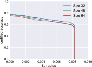
Figure 2: Certified accuracy of ResNet-110 models under varying input sizes by random smoothing.

5 Conclusions

In this paper, we show a hardness result of random smoothing on certifying adversarial robustness against attacks in the $\ell_{p}$ ball of radius $\epsilon$ when $p>2$. We focus on a lower bound on the necessary noise magnitude: any noise distribution $\mathcal{D}$ over $\mathbb{R}^{d}$ that provides $\ell_{p}$ robustness with $p>2$ for all base classifiers must satisfy $\operatorname*{\mathbb{E}}\eta_{i}^{2}=\Omega(d^{1-2/p}\epsilon^{2}(1-\delta)/\delta^{2})$ for 99% of the features (pixels) of vector $\eta$ drawn from $\mathcal{D}$, where $\delta$ is the score gap between the highest-scored class and the runner up in the framework of random smoothing. For high-dimensional images where the pixels are bounded in $[0,255]$, the required noise will eventually dominate the useful information in the images, leading to trivial smoothed classifiers.

The proof roadmap of our results shows that defending against adversarial attacks in the $\ell_{p}$ ball of radius $\epsilon$ is almost as hard as defending against attacks in the $\ell_{2}$ ball of radius $\epsilon d^{1/2-1/p}$, for random smoothing. We thus suggest combining random smoothing with dimensionality reduction techniques, such as principal component analysis or auto-encoder, to circumvent our hardness results, which is left open as future works. Another related open question is whether one can improve our lower bounds, or show that the bounds are tight.

Acknowledgments.

This work was supported in part by the National Science Foundation under grant CCF-1815011 and by the Defense Advanced Research Projects Agency under cooperative agreement HR00112020003. The views expressed in this work do not necessarily reflect the position or the policy of the Government and no official endorsement should be inferred. Approved for public release; distribution is unlimited.

Appendix A Total-Variation based Robustness

First, we argue that for any points $x$ and $x^{\prime}$, we must have $g(x)=g(x^{\prime})$ whenever the total variation distance between $\mathcal{D}+x$ and $\mathcal{D}+x^{\prime}$ is sufficiently small compared to the gap $\Delta(x)$, where $\mathcal{D}+x$ denotes the distribution of $\eta+x$ with $\eta\sim\mathcal{D}$.

Lemma A.1.

For any distribution $\mathcal{D}$ on $\mathbb{R}^{d}$, base classifier $f:\mathbb{R}^{d}\to\mathcal{Y}$, and pair of points $x,x^{\prime}\in\mathbb{R}^{d}$, if $\Delta(x)>2\operatorname{TV}(\mathcal{D}+x,\mathcal{D}+x^{\prime})$, then we have $g(x)=g(x^{\prime})$.

Proof.

To simplify notation, let $\delta=\operatorname{TV}(\mathcal{D}+x,\mathcal{D}+x^{\prime})$ and let $\eta$ be a sample from $\mathcal{D}$ so that $\eta+x$ is a sample from $\mathcal{D}+x$ and $\eta+x^{\prime}$ is a sample from $\mathcal{D}+x^{\prime}$. By the definition of the total variation distance, for any class $y\in\mathcal{Y}$, we have $\delta\geq\bigl{|}\operatorname*{Pr}\bigl{(}f(x+\eta)=y\bigr{)}-\operatorname*{Pr}\bigl{(}f(x^{\prime}+\eta)=y\bigr{)}\bigr{|}=|G_{y}(x)-G_{y}(x^{\prime})|$. Now let $y=g(x)$ and $y^{\prime}\neq y$. Then we have

$$\begin{split}G_{y}(x^{\prime})&\geq G_{y}(x)-\delta\\ &\geq G_{y^{\prime}}(x)-\delta+\Delta(x)\\ &\geq G_{y^{\prime}}(x^{\prime})-2\delta+\Delta(x).\end{split}$$

Whenever $\Delta(x)>2\delta$, we are guaranteed that $G_{y}(x^{\prime})>G_{y^{\prime}}(x^{\prime})$ for all $y^{\prime}$, and it follows that $g(x^{\prime})=y=g(x)$. ∎

As a consequence of Lemma A.1, we can provide certified robustness guarantees for the smoothed classifier $g$ in terms of balls defined by the total variation distance. In particular, for any $x\in\mathbb{R}^{d}$ and any $\delta\in(0,1]$, define

$$\mathcal{B}_{\text{TV}}(x,\delta;\mathcal{D})=\{x^{\prime}\in\mathbb{R}^{d}:\operatorname{TV}(\mathcal{D}+x,\mathcal{D}+x^{\prime})<\delta\}$$

to be the set of points $x^{\prime}$ around $x$ such that the distributions $\mathcal{D}+x$ and $\mathcal{D}+x^{\prime}$ have total variation distance at most $\delta$. When the distribution $\mathcal{D}$ is clear from context, we will simply write $\mathcal{B}_{\text{TV}}(x,\delta)$.

Corollary A.2.

For any distribution $\mathcal{D}$, base classifier $f$, and $x\in\mathbb{R}^{d}$ we have $g(x^{\prime})=g(x)$ for all $x^{\prime}\in\mathcal{B}_{\text{TV}}(x,\Delta(x)/2)$.

Note that the ball $\mathcal{B}_{\text{TV}}(x,\delta)$ is translation invariant (i.e., for any center $x\in\mathbb{R}^{d}$, we have $\mathcal{B}_{\text{TV}}(x,\delta)=\mathcal{B}_{\text{TV}}(0,\delta)+x$) and the definition of the ball only depends on the distribution $\mathcal{D}$. Therefore, if we can relate the balls for a given distribution $\mathcal{D}$ to those of a norm $\left\|\cdot\right\|_{p}$, then Corollary A.2 implies robustness with respect to that norm. Let $\mathcal{B}_{p}(x,r)=\{x^{\prime}\in\mathbb{R}^{d}:\left\|x^{\prime}-x\right\|_{p}<r\}$ denote the $\ell_{p}$ ball of radius $r$ centered at $x$.

Corollary A.3.

Fix any $p>0$, radius $\epsilon\geq 0$, distribution $\mathcal{D}$, and let $\delta\in[0,1]$ be the smallest total variation bound such that $\mathcal{B}_{p}(0,r)\subseteq\mathcal{B}_{\text{TV}}(0,\delta)$. For any base classifier $f:\mathbb{R}^{d}\to\mathcal{Y}$ and any point $x\in\mathbb{R}^{d}$ with $\Delta(x)>2\delta$, for all $x^{\prime}\in\mathcal{B}_{p}(x,r)$ we have $g(x^{\prime})=g(x)$.

The following lemma is in an opposite direction as Corollary A.3.

*

Proof.

Suppose there exists a vector $v\in\mathcal{A}$ such that $\operatorname{TV}(\mathcal{D},\mathcal{D}+v)>\delta$. We show that this implies there is a randomized binary classifier $f:\mathbb{R}^{d}\to\mathcal{Y}$, such that $g(\cdot;\mathcal{D},f)$ is not $(\mathcal{A},\delta)$-robust. It follows that if $g(\cdot;\mathcal{D},f)$ is $(\mathcal{A},\delta)$-robust for all randomized classifiers $f$, then we must have $\operatorname{TV}(\mathcal{D},\mathcal{D}+v)\leq\delta$ for all $v\in\mathcal{A}$.

Fix any $v\in\mathcal{A}$ such that $\operatorname{TV}(\mathcal{D},\mathcal{D}+v)>\delta$ and let $\mathcal{D}^{\prime}=\mathcal{D}+v$ be shorthand notation for the translated distribution. Since $\delta<\operatorname{TV}(\mathcal{D},\mathcal{D}^{\prime})=\sup_{\mathcal{S}\subseteq\mathbb{R}^{d}}\mathcal{D}(\mathcal{S})-\mathcal{D}^{\prime}(\mathcal{S})$, there exists a set $\mathcal{S}\subseteq\mathbb{R}^{d}$ so that $\mathcal{D}(\mathcal{S})-\mathcal{D}^{\prime}(\mathcal{S})>\delta$. Let $\mathcal{S}^{c}=\{x\in\mathbb{R}^{d}:x\not\in\mathcal{S}\}$ denote the complement of $\mathcal{S}$. We assume without loss of generality that $\mathcal{Y}=\{0,1\}$ and define the randomized classifier $f$ to take value $1$ with probability $\alpha$ and $0$ with probability $1-\alpha$ for all $x\in S$ and to take value $1$ with probability $\beta$ and $0$ with probability $1-\beta$ for all $x\in\mathcal{S}^{c}$, where $\alpha=1-\frac{\mathcal{D}^{\prime}(\mathcal{S})}{2}$ and $\beta=\frac{1}{2}-\frac{\mathcal{D}^{\prime}(\mathcal{S})}{2}$. That is,

$$f(x)=\begin{cases}\text{$1$ w.p. $\alpha$ and $0$ otherwise},&\text{if $x\in\mathcal{S}$};\\ \text{$1$ w.p. $\beta$ and $0$ otherwise},&\text{if $x\in\mathcal{S}^{c}$}.\end{cases}$$

Note that since $\mathcal{D}^{\prime}(\mathcal{S})\in[0,1]$ we have that $\alpha\in[\frac{1}{2},1]$ and $\beta\in[0,\frac{1}{2}]$ are both valid probabilities. For any distribution $P$ over $\mathbb{R}^{d}$ we have

$$\operatorname*{Pr}_{Z\sim P}(f(Z)=1) =\operatorname*{Pr}_{Z\sim P}\bigl{(}f(Z)=1\mid Z\in\mathcal{S}\bigr{)}\cdot P(\mathcal{S})+\operatorname*{Pr}_{Z\sim P}\bigl{(}f(Z)=1\mid Z\in\mathcal{S}^{c}\bigr{)}\cdot P(\mathcal{S}^{c})$$

$$=\alpha P(\mathcal{S})+\beta P(\mathcal{S}^{c})$$

$$=P(\mathcal{S})\cdot(\alpha-\beta)+\beta$$

$$=\frac{1}{2}+\frac{P(\mathcal{S})-\mathcal{D}^{\prime}(\mathcal{S})}{2}.$$

Therefore, we have $G_{1}(0;\mathcal{D},f)=\operatorname*{Pr}_{Z\sim\mathcal{D}}\bigl{(}f(Z)=1\bigr{)}=\frac{1}{2}+\frac{\mathcal{D}(\mathcal{S})-\mathcal{D}^{\prime}(\mathcal{S})}{2}>\frac{1}{2}+\frac{\delta}{2}$. Similarly, we have that $G_{1}(v;\mathcal{D},f)=\operatorname*{Pr}_{Z\sim\mathcal{D}}\bigl{(}f(Z+v)=1\bigr{)}=\operatorname*{Pr}_{Z\sim\mathcal{D}^{\prime}}\bigl{(}f(Z)=1\bigr{)}=\frac{1}{2}$. It follows that $g(0;\mathcal{D},f)=1$, $\Delta(0;\mathcal{D},f)=2G_{1}(0;\mathcal{D},f)-1>2(\frac{1}{2}+\frac{\delta}{2})-1=\delta$, and $g(v;\mathcal{D},f)=0$ (since $G_{1}(v;\mathcal{D},f)=G_{0}(v;\mathcal{D},f)=\frac{1}{2}$ and the ties are broken lexicographically). It follows that $g(\cdot;\mathcal{D},f)$ is not robust to the adversarial translation $v\in\mathcal{A}$, as required. ∎

Appendix B Total Variation Bounds for Specific Distributions

B.1 Isotropic Gaussian

In this section we give bounds for the total variation distance between shifted copies of Gaussian distributions with an isotropic covariance matrix. Our results are derived from the following theorem due to Devroye et al. (2018).

Theorem B.1 (Theorem 1.2 of Devroye et al. (2018)).

Suppose $d>1$, let $\mu_{1}\neq\mu_{2}\in\mathbb{R}^{d}$ and let $\Sigma_{1},\Sigma_{2}$ be positive definite $d\times d$ matrices. Let $v=\mu_{1}-\mu_{2}$ and let $\Pi$ be a $d\times d-1$ matrix whose columns form a basis for the subspace orthogonal to $v$. Define the function

$$tv(\mu_{1},\Sigma_{1},\mu_{2},\Sigma_{2})=\max\Bigg{\{}\left\|(\Pi^{\top}\Sigma_{1}\Pi)^{-1}\Pi^{\top}\Sigma_{2}\Pi-I_{d-1}\right\|_{F},\frac{|v^{\top}(\Sigma_{1}-\Sigma_{2})v|}{v^{\top}\Sigma_{1}v},\frac{v^{\top}v}{\sqrt{v^{\top}\Sigma_{1}v}}\Bigg{\}},$$

where $\left\|\cdot\right\|_{F}$ denotes the Frobenius norm and $I_{d-1}$ is the $(d-1)$-dimensional identity matrix. Then we have

$$\frac{1}{200}\leq\frac{\operatorname{TV}(\mathcal{N}(\mu_{1},\Sigma_{1}),\mathcal{N}(\mu_{2},\Sigma_{2}))}{\min\{1,tv(\mu_{1},\Sigma_{1},\mu_{2},\Sigma_{2})\}}\leq\frac{9}{2}.$$

Theorem B.1 takes a simpler form when $\Sigma_{1}=\Sigma_{2}=\sigma^{2}I$ and $\mu_{1}=0$ because then the first and last terms in the max of $tv(\mu_{1},\Sigma_{1},\mu_{2},\Sigma_{2})$ are zero, giving the following:

Corollary B.2.

Suppose $d>1$ and let $v\in\mathbb{R}^{d}$ and $\sigma>0$. Then

$$\begin{split}\frac{1}{200}\cdot\min\left\{1,\frac{\left\|v\right\|_{2}}{\sigma}\right\}&\leq\operatorname{TV}\bigl{(}\mathcal{N}(0,\sigma^{2}I),\mathcal{N}(v,\sigma^{2}I)\bigr{)}\leq\frac{9}{2}\cdot\min\left\{1,\frac{\left\|v\right\|_{2}}{\sigma}\right\}.\end{split}$$

We can use this result to show that the variance bounds given by Lemma 3.7 are nearly tight, except for the dependence on the total variation bound, $\delta$.

Corollary B.3.

Fix any $d$, radius $\epsilon>0$, total variation bound $\delta\in[0,1]$, and $p\geq 2$. Setting $\sigma=\frac{9}{2}\frac{\epsilon}{\delta}d^{1/2-1/p}$ guarantees that for all $v\in\mathbb{R}^{d}$ with $\left\|v\right\|_{p}\leq\epsilon$ we have $\operatorname{TV}(\mathcal{N}(0,\sigma^{2}I),\mathcal{N}(v,\sigma^{2}I))\leq\delta$. Moreover, if $\eta\sim\mathcal{N}(0,\sigma^{2}I)$ then $\operatorname*{\mathbb{E}}[\eta_{i}^{2}]=\sigma^{2}=(\frac{9}{2})^{2}\cdot\frac{\epsilon^{2}}{\delta^{2}}\cdot d^{1-2/p}$ and $\operatorname*{\mathbb{E}}[\left\|\eta\right\|_{2}]\leq\frac{9}{2}\frac{\epsilon}{\delta}\cdot d^{1-1/p}$.

Proof.

Since for every $v\in\mathbb{R}^{d}$ with $\left\|v\right\|_{p}\leq\epsilon$ we have $\left\|v\right\|_{2}\leq\epsilon\cdot d^{1/2-1/p}$, it is sufficient to choose $\sigma$ as in the statement. To bound $\operatorname*{\mathbb{E}}[\left\|\eta\right\|_{2}]$, we use Jensen’s inequality: $\operatorname*{\mathbb{E}}[\left\|\eta\right\|_{2}]\leq\sqrt{\operatorname*{\mathbb{E}}[\left\|\eta\right\|_{2}^{2}]}=\sqrt{d}\sigma=\frac{9}{2}\frac{\epsilon}{\delta}d^{1-1/p}$. ∎

B.2 Uniform Distribution on $\mathcal{B}_{\infty}(0,r)$

In this section, let $\mathcal{U}_{r}$ denote the uniform distribution on $\mathcal{B}_{\infty}(0,r)$ with density $p_{r}(x)=\frac{1}{(2r)^{d}}\operatorname{\mathbb{I}}\{x\in\mathcal{B}_{\infty}(0,r)\}$.

Lemma B.4.

For any dimension $d$, any vector $v\in\mathbb{R}^{d}$, and any radius $r\geq 0$, we have

$$\operatorname{TV}(\mathcal{U}_{r},\mathcal{U}_{r}+v)=1-\prod_{i=1}^{d}\max\left\{0,1-\frac{|v_{i}|}{2r}\right\}.$$

Proof.

To simplify notation, let $\mathcal{A}=\mathcal{B}_{\infty}(0,r)$ and $\mathcal{B}=\mathcal{B}_{\infty}(v,r)$. Since $\mathcal{U}_{r}$ has a density function, we can write the total variation distance as

$$\begin{split}\operatorname{TV}(\mathcal{U}_{r},\mathcal{U}_{r}+v)&=\frac{1}{2}\int_{\mathbb{R}^{d}}|p_{r}(x)-p_{r}(x-v)|\,dx\\ &=\frac{1}{2}(2r)^{-d}\int_{\mathbb{R}^{d}}|\operatorname{\mathbb{I}}\{x\in\mathcal{A}\}-\operatorname{\mathbb{I}}\{x\in\mathcal{B}\}|\,dx\\ &=\frac{1}{2}(2r)^{-d}\operatorname{Vol}(\mathcal{A}\triangle\mathcal{B}),\end{split}$$

where $\mathcal{A}\triangle\mathcal{B}$ denotes the symmetric difference of $\mathcal{A}$ and $\mathcal{B}$. Since $\operatorname{Vol}(\mathcal{A}\triangle\mathcal{B})=\operatorname{Vol}(\mathcal{A})+\operatorname{Vol}(\mathcal{B})-2\operatorname{Vol}(\mathcal{A}\cap\mathcal{B})$, it is sufficient to calculate the volume of $\mathcal{A}\cap\mathcal{B}$. The intersection is a hyper-rectangle with side length $\max\{0,2r-|v_{i}|\}$ in dimension $i$. Therefore, the volume of the intersection is given by $\operatorname{Vol}\bigl{(}\mathcal{A}\cap\mathcal{B})=\prod_{i=1}^{d}\max\{0,2r-|v_{i}|\}$. Combined with the fact that $\operatorname{Vol}(\mathcal{A})=\operatorname{Vol}(\mathcal{B})=(2r)^{d}$ this gives

$$\begin{split}\operatorname{TV}(\mathcal{U}_{r},\mathcal{U}_{r}+v)&=\frac{1}{(2r)^{d}}\left((2r)^{d}-\prod_{i}\max\{0,2r-|v_{i}|\}\right)\\ &=1-\prod_{i}\max\left\{0,1-\frac{|v_{i}|}{2r}\right\},\end{split}$$

as required. ∎

We can also compute the TV-distance for the worst-case shift $v$ with $\left\|v\right\|_{\infty}\leq\epsilon$.

Corollary B.5.

For any $\epsilon\geq 0$, the vector $v=(\epsilon,\dots,\epsilon)\in\mathbb{R}^{d}$ satisfies

$$v\in\operatorname*{argmax}_{v:\left\|v\right\|_{\infty}\leq\epsilon}\operatorname{TV}(\mathcal{U}_{r},\mathcal{U}_{r}+v),$$

and $\operatorname{TV}(\mathcal{U}_{r},\mathcal{U}_{r}+v)=\min\{1,1-(1-\frac{\epsilon}{2r})^{d}\}$. Finally, for $\epsilon\in[0,r]$, we have

$$1-e^{-\frac{d\epsilon}{2r}}\leq\max_{v:\left\|v\right\|_{\infty}\leq\epsilon}\operatorname{TV}(\mathcal{U}_{r},\mathcal{U}_{r}+v)\leq 1-4^{-\frac{d\epsilon}{2r}}.$$

Proof.

To see that $v=(\epsilon,\dots,\epsilon)$ is a maximizer, observe that the optimization problem decouples over the components $v_{i}$ and that to maximize the term corresponding to component $v_{i}$ we want to choose $|v_{i}|$ as large as possible. It follows that all vectors $v\in\{\pm\epsilon\}^{d}$ are maximizers.

The bounds for when $\epsilon\in[0,r]$ follow from the fact that for any $z\in[0,\frac{1}{2}]$, we have $4^{-x}\leq 1-z\leq e^{-z}$ applied with $z=1-\frac{\epsilon}{2r}$. ∎

Corollary B.6.

Fix any dimension $d$, radius $\epsilon>0$, and total variation bound $\delta\in[0,1]$. Setting $r=\frac{1}{2}\frac{\epsilon}{\delta}d\log(4)$ guarantees that for all $v\in\mathbb{R}^{d}$ such that $\left\|v\right\|_{\infty}\leq\epsilon$ we have $\operatorname{TV}(\mathcal{U}_{r},\mathcal{U}_{r}+v)\leq\delta$. Moreover, if $\eta\sim\mathcal{U}_{r}$ then $\operatorname*{\mathbb{E}}[\eta_{i}^{2}]$ is the variance of a uniform random variable on $[-r,r]$, which is $\frac{\sqrt{2}\log(4)^{2}}{48}\frac{\epsilon^{2}}{\delta^{2}}d^{2}\leq\frac{\epsilon^{2}}{\delta^{2}}d^{2}$.

Proof.

This follows by determining the smallest value of $r$ for which $1-4^{-\frac{d\epsilon}{2\delta}}\leq\delta$. ∎

Appendix C Lower Bound on Noise $\ell_{2}$-Norm

Lemma C.1.

Fix any $p\geq 2$ and let $\mathcal{D}$ be a distribution on $\mathbb{R}^{d}$ such that there exists a radius $\epsilon$ and total variation bound $\delta$ satisfying that for all $v\in\mathbb{R}^{d}$ with $\left\|v\right\|_{p}\leq\epsilon$ we have $\operatorname{TV}(\mathcal{D},\mathcal{D}+v)\leq\delta$. Then

$$\operatorname*{\mathbb{E}}_{\eta\sim\mathcal{D}}\left\|\eta\right\|_{2}\geq\frac{\epsilon d^{1-1/p}}{24}\cdot\frac{1-\delta}{\delta}.$$

Proof.

We first prove the lemma in the one-dimensional case. Let $\eta^{\prime}=\eta+\epsilon\in\mathbb{R}$ so that $\eta^{\prime}$ is a sample from $\mathcal{D}+\epsilon$ and define $r=\epsilon/2$ so that the sets $\mathcal{A}=(-r,r)$ and $\mathcal{B}=(\epsilon-r,\epsilon+r)$ are disjoint. From Markov’s inequality, we have that $\operatorname*{Pr}(\eta\in\mathcal{A})=1-\operatorname*{Pr}(|\eta|\geq r)\geq 1-\frac{\operatorname*{\mathbb{E}}|\eta|}{r}$. Further, since $\eta^{\prime}\in\mathcal{B}$ if and only if $\eta\in\mathcal{A}$, we have $\operatorname*{Pr}(\eta^{\prime}\in\mathcal{B})\geq 1-\frac{\operatorname*{\mathbb{E}}|\eta|}{r}$. Next, since $\mathcal{A}$ and $\mathcal{B}$ are disjoint, it follows that $\operatorname*{Pr}(\eta^{\prime}\in\mathcal{A})\leq 1-\operatorname*{Pr}(\eta^{\prime}\in\mathcal{B})\leq 1-1+\frac{\operatorname*{\mathbb{E}}|\eta|}{r}=\frac{\operatorname*{\mathbb{E}}|\eta|}{r}$. Finally, we have $\delta\geq\operatorname*{Pr}(\eta\in\mathcal{A})-\operatorname*{Pr}(\eta^{\prime}\in\mathcal{A})\geq 1-\frac{2\operatorname*{\mathbb{E}}|\eta|}{r}=1-\frac{4\operatorname*{\mathbb{E}}|\eta|}{\epsilon}$. Rearranging this inequality proves the claim that $\mathbb{E}|\eta|\geq(1-\delta)\epsilon/4$. Combining with Lemma 3.3, we obtain that $\operatorname*{\mathbb{E}}|\eta|\geq\frac{\epsilon}{12}\cdot\frac{1-\delta}{\delta}$, due to the fact that for any $\delta\in(0,1]$ we have $\max\{\frac{1-\delta}{4},\frac{(1-\delta)^{2}}{8\delta}\}\geq\frac{1}{12}\cdot\frac{1-\delta}{\delta}$.

We now prove the $d$-dimensional case. Let $\eta$ be a sample from $\mathcal{D}$. By scaling the vectors from Corollary 3.6 by $\epsilon$, we obtain $b>d/2$ vectors $v_{1},\dots,v_{b}\in\mathbb{R}^{d}$ with $\left\|v_{i}\right\|_{p}=\epsilon$ and $\left\|v_{i}\right\|_{2}=\epsilon\cdot b^{1/2-1/p}$. By assumption we must have $\operatorname{TV}(\mathcal{D},\mathcal{D}+v_{i})\leq\delta$, since $\left\|v_{i}\right\|_{p}\leq\epsilon$, and the above-mentioned one-dimensional case implies that $\operatorname*{\mathbb{E}}\frac{|v_{i}^{\top}\eta|}{\left\|v_{i}\right\|_{2}}\geq\frac{\left\|v_{i}\right\|_{2}}{12}\frac{1-\delta}{\delta}$ for each $i$. We use this fact to bound $\operatorname*{\mathbb{E}}\left\|\eta\right\|_{2}$.

Let $\mathbf{Q}\in\mathbb{R}^{b\times d}$ be the matrix whose $i^{\text{th}}$ row is given by $v_{i}/\left\|v_{i}\right\|_{2}$ so that $\mathbf{Q}$ is the orthogonal projection matrix onto the subspace spanned by the vectors $v_{1},\dots,v_{b}$. Then we have

$$\operatorname*{\mathbb{E}}\left\|\eta\right\|_{2}\geq\operatorname*{\mathbb{E}}\left\|\mathbf{Q}\eta\right\|_{2}\geq\frac{1}{\sqrt{b}}\operatorname*{\mathbb{E}}\left\|\mathbf{Q}\eta\right\|_{1}=\frac{1}{\sqrt{b}}\sum_{i=1}^{b}\operatorname*{\mathbb{E}}\frac{|v_{i}^{\top}\eta|}{\left\|v_{i}\right\|_{2}}\geq\frac{1}{\sqrt{b}}\sum_{i=1}^{b}\frac{\left\|v_{i}\right\|_{2}}{12}\frac{1-\delta}{\delta},$$

where the first inequality follows because orthogonal projections are non-expansive, the second inequality follows from the equivalence of $\ell_{2}$ and $\ell_{1}$ norms, and the last inequality follows from $\operatorname*{\mathbb{E}}\frac{|v_{i}^{\top}\eta|}{\left\|v_{i}\right\|_{2}}\geq\frac{\left\|v_{i}\right\|_{2}}{12}\frac{1-\delta}{\delta}$. Using the fact that $\left\|v_{i}\right\|_{2}=\epsilon\cdot b^{1/2-1/p}$, we have that $\operatorname*{\mathbb{E}}\left\|\eta\right\|_{2}\geq\frac{\epsilon b^{1-1/p}}{12}\cdot\frac{1-\delta}{\delta}$. Finally, since $b>d/2$ and $(1/2)^{1-1/p}\geq 1/2$ for $p\geq 2$, we have $\operatorname*{\mathbb{E}}\left\|\eta\right\|_{2}\geq\frac{\epsilon d^{1-1/p}}{24}\cdot\frac{1-\delta}{\delta}$, as required. ∎

References

- Athalye et al. (2018) Anish Athalye, Nicholas Carlini, and David Wagner. Obfuscated gradients give a false sense of security: Circumventing defenses to adversarial examples. In International Conference on Machine Learning, 2018.
- Brendel et al. (2020) Wieland Brendel, Jonas Rauber, Alexey Kurakin, Nicolas Papernot, Behar Veliqi, Sharada P Mohanty, Florian Laurent, Marcel Salathé, Matthias Bethge, Yaodong Yu, Hongyang Zhang, et al. Adversarial vision challenge. In The NeurIPS’18 Competition, pages 129–153. Springer, 2020.
- Brown et al. (2018) Tom B Brown, Nicholas Carlini, Chiyuan Zhang, Catherine Olsson, Paul Christiano, and Ian Goodfellow. Unrestricted adversarial examples. arXiv preprint arXiv:1809.08352, 2018.
- Cohen et al. (2019) Jeremy M Cohen, Elan Rosenfeld, and J Zico Kolter. Certified adversarial robustness via randomized smoothing. In International Conference on Machine Learning, 2019.
- Devroye et al. (2018) Luc Devroye, Abbas Mehrabian, and Tommy Reddad. The total variation distance between high-dimensional Gaussians. arXiv preprint arXiv:1810.08693, 2018.
- Dvijotham et al. (2020) Krishnamurthy (Dj) Dvijotham, Jamie Hayes, Borja Balle, Zico Kolter, Chongli Qin, Andras Gyorgy, Kai Xiao, Sven Gowal, and Pushmeet Kohli. A framework for robustness certification of smoothed classifiers using f-divergences. In International Conference on Learning Representations, 2020.
- Gowal et al. (2018) Sven Gowal, Krishnamurthy Dvijotham, Robert Stanforth, Rudy Bunel, Chongli Qin, Jonathan Uesato, Relja Arandjelovic, Timothy Mann, and Pushmeet Kohli. On the effectiveness of interval bound propagation for training verifiably robust models. arXiv preprint arXiv:1810.12715, 2018.
- He et al. (2016) Kaiming He, Xiangyu Zhang, Shaoqing Ren, and Jian Sun. Deep residual learning for image recognition. In IEEE conference on computer vision and pattern recognition, pages 770–778, 2016.
- Jia et al. (2020) Jinyuan Jia, Xiaoyu Cao, Binghui Wang, and Neil Zhenqiang Gong. Certified robustness for top-k predictions against adversarial perturbations via randomized smoothing. In International Conference on Learning Representations, 2020.
- Lecuyer et al. (2019) Mathias Lecuyer, Vaggelis Atlidakis, Roxana Geambasu, Daniel Hsu, and Suman Jana. Certified robustness to adversarial examples with differential privacy. In IEEE Symposium on Security and Privacy, pages 656–672, 2019.
- Lee et al. (2019) Guang-He Lee, Yang Yuan, Shiyu Chang, and Tommi Jaakkola. Tight certificates of adversarial robustness for randomly smoothed classifiers. In Advances in Neural Information Processing Systems, pages 4911–4922, 2019.
- Li et al. (2019) Bai Li, Changyou Chen, Wenlin Wang, and Lawrence Carin. Certified adversarial robustness with additive noise. In Advances in Neural Information Processing Systems, pages 9459–9469, 2019.
- Madry et al. (2017) Aleksander Madry, Aleksandar Makelov, Ludwig Schmidt, Dimitris Tsipras, and Adrian Vladu. Towards deep learning models resistant to adversarial attacks. arXiv preprint arXiv:1706.06083, 2017.
- Mirman et al. (2018) Matthew Mirman, Timon Gehr, and Martin Vechev. Differentiable abstract interpretation for provably robust neural networks. In International Conference on Machine Learning, pages 3578–3586, 2018.
- Raghunathan et al. (2018) Aditi Raghunathan, Jacob Steinhardt, and Percy S Liang. Semidefinite relaxations for certifying robustness to adversarial examples. In Advances in Neural Information Processing Systems, pages 10877–10887, 2018.
- Salman et al. (2019) Hadi Salman, Jerry Li, Ilya Razenshteyn, Pengchuan Zhang, Huan Zhang, Sebastien Bubeck, and Greg Yang. Provably robust deep learning via adversarially trained smoothed classifiers. In Advances in Neural Information Processing Systems, pages 11289–11300, 2019.
- Szegedy et al. (2013) Christian Szegedy, Wojciech Zaremba, Ilya Sutskever, Joan Bruna, Dumitru Erhan, Ian Goodfellow, and Rob Fergus. Intriguing properties of neural networks. arXiv preprint arXiv:1312.6199, 2013.
- Vershynin (2018) Roman Vershynin. High-dimensional probability: An introduction with applications in data science, volume 47. Cambridge university press, 2018.
- Wong et al. (2018) Eric Wong, Frank Schmidt, Jan Hendrik Metzen, and J Zico Kolter. Scaling provable adversarial defenses. In Advances in Neural Information Processing Systems, pages 8400–8409, 2018.
- Wong et al. (2019) Eric Wong, Frank R Schmidt, and J Zico Kolter. Wasserstein adversarial examples via projected Sinkhorn iterations. In International Conference on Machine Learning, 2019.
- Xiao et al. (2019) Kai Y Xiao, Vincent Tjeng, Nur Muhammad Shafiullah, and Aleksander Madry. Training for faster adversarial robustness verification via inducing ReLU stability. In International Conference on Learning Representations, 2019.
- Yang et al. (2019) Xiao Yang, Fangyun Wei, Hongyang Zhang, Xiang Ming, and Jun Zhu. Design and interpretation of universal adversarial patches in face detection. arXiv preprint arXiv:1912.05021, 2019.
- Zhai et al. (2020) Runtian Zhai, Chen Dan, Di He, Huan Zhang, Boqing Gong, Pradeep Ravikumar, Cho-Jui Hsieh, and Liwei Wang. MACER: Attack-free and scalable robust training via maximizing certified radius. In International Conference on Learning Representations, 2020.
- Zhang et al. (2019) Hongyang Zhang, Yaodong Yu, Jiantao Jiao, Eric P Xing, Laurent El Ghaoui, and Michael I Jordan. Theoretically principled trade-off between robustness and accuracy. In International Conference on Machine Learning, 2019.
- Zhang et al. (2020) Huan Zhang, Hongge Chen, Chaowei Xiao, Bo Li, Duane Boning, and Cho-Jui Hsieh. Towards stable and efficient training of verifiably robust neural networks. In International Conference on Learning Representations, 2020.