Fast radio bursts from activities of neutron stars newborn in BNS mergers: offset, birth rate and observational properties

Abstract

Young neutron stars (NSs) born in core-collapse explosions are promising candidates for the central engines of fast radio bursts (FRBs), since the first localized repeating burst FRB 121102 happens in a star forming dwarf galaxy, which is similar to the host galaxies of superluminous supernovae (SLSNe) and long gamma-ray bursts (LGRBs). However, FRB 180924 and FRB 190523 are localized to massive galaxies with low rates of star formation, compared with the host of FRB 121102. Meanwhile, the offsets between the bursts and host centers are about 4 kpc and 29 kpc for FRB 180924 and FRB 190523, respectively. These properties of hosts are similar to short gamma-ray bursts (SGRBs), which are produced by mergers of binary neutron star (BNS) or neutron star-black hole (NS-BH). Therefore, the NSs powering FRBs may be formed in BNS mergers. In this paper, we study the BNS merger rates, merger times, and predict their most likely merger locations for different types of host galaxies using population synthesis method. We find that the BNS merger channel is consistent with the recently reported offsets of FRB 180924 and FRB 190523. The offset distribution of short GRBs is well reproduced by population synthesis using galaxy model which is similar to GRB hosts. The event rate of FRBs (including non-repeating and repeating), is larger than those of BNS merger and short GRBs, which requires a large fraction of observed FRBs emitting several bursts. Using curvature radiation by bunches in NS magnetospheres, we also predict the observational properties of FRBs from BNS mergers, including the dispersion measure, and rotation measure. At late times ($t\geq 1$yr), the contribution to dispersion measure and rotation measure from BNS merger ejecta could be neglected.

1 Introduction

Fast radio bursts (FRBs) are transients of coherent emission lasting about a few milliseconds (Lorimer et al., 2007; Thornton et al., 2013; Champion et al., 2016; Shannon et al., 2018; Platts et al., 2019; Petroff et al., 2019; Cordes & Chatterjee, 2019) with large dispersion measures (DMs). Thanks to multi-wavelength follow-up observations and a precise localization, the repeating FRB 121102 was localized in a dwarf star-forming galaxy at $z=0.19$ (Chatterjee et al., 2017; Tendulkar et al., 2017; Marcote et al., 2017). This FRB is also spatially associated with a persistent radio source (Chatterjee et al., 2017; Marcote et al., 2017). The properties of this galaxy is similar to the host galaxies of superluminous supernovae (SLSNe) and long gamma-ray bursts (LGRBs) (Tendulkar et al., 2017; Metzger et al., 2017; Nicholl et al., 2017; Zhang & Wang, 2019). This has led to the hypothesis that bursts are produced by young active neutron stars (NSs) (Popov & Postnov, 2013; Lyubarsky, 2014; Kulkarni et al., 2014; Katz, 2016b; Lu & Kumar, 2016; Murase et al., 2016; Wang & Yu, 2017; Metzger et al., 2017; Beloborodov, 2017; Lu & Kumar, 2018; Yang & Zhang, 2018; Wang & Lai, 2019; Beloborodov, 2019; Cheng et al., 2020). The young active NSs are born in core-collapse explosions. Recently, a second repeating FRB 180916.J0158+65 was localized to a star-forming region in a nearby massive spiral galaxy (Marcote et al., 2020). Two coherent mechanisms are often considered in current FRB models: curvature radiation by bunches (Katz, 2014, 2018a; Kumar et al., 2017; Ghisellini & Locatelli, 2018; Yang & Zhang, 2018) and the maser mechanisms (Lyubarsky, 2014; Beloborodov, 2017; Ghisellini, 2017; Waxman, 2017; Lu & Kumar, 2018; Metzger et al., 2019; Beloborodov, 2019).

Recently, two FRBs, which are both single bursts, have been localized to massive galaxies by the Australian Square Kilometre Array Pathfinder (ASKAP) and Deep Synoptic Array ten-antenna prototype (DSA-10) respectively. FRB 180924 occured in a massive galaxy at redshift $z=0.32$ with lower star formation rate (Bannister et al., 2019). The offset between the burst and host galaxy center is about 4 kpc (Bannister et al., 2019). The DM contributed by host galaxy of FRB 180924 is small (between 30-81 pc cm^-3), which makes FRBs become a promising cosmological probe (Gao et al., 2014; Zhou et al., 2014; Wei et al., 2015; Yang & Zhang, 2016; Yu & Wang, 2017; Walters et al., 2018; Wang & Wang, 2018; Li et al., 2018; Yu & Wang, 2018; Zhang, 2018a; Li et al., 2019b; Liu et al., 2019). The Deep Synoptic Array ten-antenna prototype (DSA-10) localized FRB 190523 to a massive galaxy at a redshift of 0.66 (Ravi et al., 2019). This galaxy is different from the host of FRB 121102, as it is about a thousand times more massive, with a specific star formation rate two orders of magnitude lower (Ravi et al., 2019). Aside from the two confirmed host galaxies, Li et al. (2019a) recently found that the host candidates of some nearby FRBs are also not similar to that of FRB 121102. This low star formation rate and large offset of FRB hosts indicate that the NSs powering FRBs may be formed by mergers of binary neutron stars (BNSs), which is similar to short GRBs. Observationally, short GRBs occur in early-type galaxies with low star formation (Barthelmy et al., 2005; Gehrels et al., 2005; Bloom et al., 2006) and have large offsets from the centers of the host galaxies (Fox et al., 2005; Fong et al., 2013). Some short GRBs show X-ray flares and internal plateaus with rapid decay at the end of the plateaus, which are consistent with a millisecond NS born in BNS merger (Dai et al., 2006; Metzger et al., 2008; Rowlinson et al., 2013; Wang & Dai, 2013; Lü et al., 2015).

There are at least two distinct NSs formation channels, i.e., core-collapse explosions and BNS mergers. The BNS merger channel is different from the core-collapse explosion channel in two aspects. First, the ejecta produced by BNS merger has higher velocity ($v\sim(0.1-0.3)c$) and lower mass (($10^{-4}-10^{-2})M_{\odot}$), compared with that of core-collapse explosion. The ejecta can affect the observational properties of FRBs (Margalit et al., 2019). Second, the offsets in the two cases are different. At the time of birth, NSs receive natal kicks, which are connected to asymmetries in supernova explosions. Due to the long delay time, BNS will merge at large radius in host galaxies even if born at small radius (Bloom et al., 1999; Fryer et al., 1999; Belczynski et al., 2006). However, in our population synthesis, most of primary neutron stars receive small kicks (see Sec. 2.6 for details). Margalit et al. (2019) also studied the properties of FRBs from magnetars born in BNS mergers and accretion induced collapse.

In this paper, we perform an updated analysis of BNS mergers using population synthesis methods (Bloom et al., 1999; Fryer et al., 1999; Belczynski et al., 2002; Perna & Belczynski, 2002; Voss & Tauris, 2003; Belczynski et al., 2006) and calculate the FRB properties from BNS mergers. Compared with previous population synthesis codes (Hurley et al., 2002; Belczynski et al., 2008), the new version of binary star evolution ($\mathtt{BSE}$) code (Banerjee et al., 2019) includes several major upgrades. The most important one is the new formation channel of NSs from electron-capture supernova (ECS). For close binaries, stars with masses between $(6-8)~{}M_{\odot}$ can form ECS-NSs (Podsiadlowski et al., 2004). We also show the properties of FRBs powering by NSs from BNS mergers using curvature radiation by bunches (Yang & Zhang, 2018).

The paper is structured as follows. The description of binary-star-evolution (BSE) code, galaxy potential models, and kick velocity are presented in section 2. The results of population synthesis, including merger time and delay time distributions, offsets distribution and merger rate, are given in section 3. In section 4, we compare the event rates of FRBs, short GRBs and BNS mergers. The observational properties of FRBs from NS formed by BNS mergers are shown in section 5. Conclusions and discussion are given in section 6.

2 Compact binaries from population synthesis

2.1 The $\mathtt{BSE}$ code

The $\mathtt{BSE}$ code, developed by Jarrod Hurley, Onno Pols and Christopher Tout, is a rapid binary-evolution algorithm based on a suite of analytical formulae (Hurley et al., 2002). It is incorporated into the N-body evolution program $\mathtt{NBODY7}$ (Aarseth, 2012) for globular cluster as the stellar-evolutionary sector. Three major upgrades are added to the new version of $\mathtt{BSE}$ code (Banerjee et al., 2019), including (i) the semi-empirical stellar wind prescriptions (Belczynski et al., 2010), (ii) remnant formation and material fallback (Fryer et al., 2012) and the occurrences of pair-instability supernova (PSN) and pulsation pair-instability supernova (PPSN) (Belczynski et al., 2016), and (iii) a modulation of the BHs’ and the NSs’ natal kicks based on the fallback fraction during their formation (Banerjee et al., 2019).

The new $\mathtt{BSE}$ code includes the electron-capture-supernovae (ECS)-NS formation channel (Podsiadlowski et al., 2004; Belczynski et al., 2008) compared to the previous version (Hurley et al., 2002). The primary star in binary system with initial mass in the range $6-8~{}M_{\odot}$ is likely to become an electron-capture supernova (Podsiadlowski et al., 2004), producing the ECS-NS, which typically has so small ($<$ 20 km/s) or zero kick velocity that remains bound to globular clusters whose escape velocities are 10–20 km/s (Katz, 1975). These NSs are distinctly least massive NSs, born with characteristic mass $m_{\mathrm{ECS},\mathrm{NS}}=1.26M_{\odot}$ (Banerjee et al., 2019).

Besides, we adopt the remnant-mass prescription of Belczynski et al. (2002) ($\mathtt{nsflag}=1$), no PPSN/PSN mass cutoff ($\mathtt{psflag}=0$) and standard, momentum-conserving kick of Belczynski et al. (2008) ($\mathtt{kmech}=1$). The program $\mathtt{popbin}$ is used to carry out the population synthesis.

2.2 Parameter distribution

We created a catalog of 1000,000 binary systems in which the the initial system parameters ($M_{1},q,e,P$) satisfy the following distributions

$$f_{M_{1}}\left(M_{1}\right)\propto{M_{1}^{-\alpha},}\qquad{\text{ for }M_{1}\in[5,100]}$$ (1)

$$f_{q}(q)\propto q^{\kappa},\qquad\text{ for }q\in[0.1,1]$$ (2)

$$f_{e}(e)\propto e^{\eta},\qquad\text{ for }e\in[0.0,1.0]$$ (3)

$$f_{P}(\log_{10}P)\propto(\log_{10}P)^{\pi},\qquad\text{ for }\log_{10}P\in[0.15,5.5]$$ (4)

where $M_{1}$ is the mass of the primary star, $\alpha=2.7$ (Scalo, 1986); $q\equiv m_{2}/m_{1}$ is the mass ratio of the two stars; $P$ and $e$ are orbital period and eccentivity respectively; $\kappa=0$ (Bethe & Brown, 1998), $\eta=1$ (Duquennoy & Mayor, 1991) and $\pi=0.5$ (Sana et al., 2012) are used in our simulation. It is worth mentioning that the initial binary properties do not significantly affect (within a factor of 2) the predictions of double compact object merger rates (de Mink & Belczynski, 2015). The metallicity $Z$ and maximum evolution time $T$ are set to 0.02 and $15,000\text{ Myr}$ for all binaries.

2.3 Motion of binaries in the gravitational field of the galaxy

To obtain the predicted offset of the binary compact objects merger, we need to know the motion of the binary, which depends on its initial locations and velocity, the gravitational field of the galaxy, the kick velocity as well as the delay time. Here, we consider the spiral galaxy and elliptical galaxy with different sizes.

For a spiral galaxy, there are three components: a disk, a bulge and a halo. The galactic disk and bulge potential was proposed by Miyamoto & Nagai (1975)

$$\Phi_{i}(R,z)=-\frac{GM_{i}}{\sqrt{R^{2}+\left(a_{i}+\sqrt{z^{2}+b_{i}^{2}}\right)^{2}}},$$ (5)

where $\Phi_{1}$ and $\Phi_{2}$ refer to bulge and disk potential respectively. The bulge potential $\Phi_{1}$ is described by $M_{1}=1.0\times 10^{10}M_{\odot}$, $a_{1}=0$ and $b_{1}=0.267\text{ kpc}$; the disk potential $\Phi_{2}$ is described by $M_{2}=6.5\times 10^{10}M_{\odot}$, $a_{2}=4.4\text{ kpc}$ and $b_{2}=0.308\text{ kpc}$ (Bajkova & Bobylev, 2017).

For an elliptical galaxy, only bulge and halo are considered. The bulge potential model is Hernquist model (Hernquist, 1990)

$$\Phi(r)=-\frac{GM_{e}}{r+a_{e}},$$ (6)

where $M_{e}=5\times 10^{11}M_{\odot}$ and $a_{e}=5\text{ kpc}$ (Belczynski et al., 2006).

The halo potential for both spiral galaxy and elliptical galaxy is given by Navarro-Frenk-White (NFW) profile (Navarro et al., 1996)

$$\Phi_{\mathrm{h}}(r)=-\frac{GM_{\mathrm{h}}}{r}\ln\bigg{(}1+\frac{r}{a_{\mathrm{h}}}\bigg{)},$$ (7)

where $M_{h}=2.9\times 10^{11}M_{\odot}$ and $a_{h}=7.7\text{ kpc}$ are provided by Bajkova & Bobylev (2017).

2.4 Initial conditions

The cylindrical coordinates $(R_{0},z_{0})$ of initial location of the binary obey the following distributions

$$p_{R}(R)\propto R\mathrm{e}^{-R/R_{\mathrm{exp}}},$$ (8)

$$p_{z}(z)\propto\mathrm{e}^{-|z|/z_{\mathrm{exp}}},$$ (9)

where $R_{\mathrm{exp}}=4.5\text{ kpc}$, $R_{\mathrm{max}}=20\text{ kpc}$, $z_{\mathrm{exp}}=75\text{ pc}$ and $z_{\mathrm{max}}=300\text{ pc}$ is used (Paczynski, 1990). For a galaxy with different size, a scale factor $\alpha$ is used to change the mass and spatial size proportionally, i.e., $M^{\prime}=\alpha M$, $R^{\prime}=\alpha^{1/3}R$ (Belczynski et al., 2002), where $M$ and $R$ are typical mass and spatial size of a Milky-Way-like galaxy. In this study, $\alpha=1,0.1,0.01,0.001$ are considered.

The initial velocity $v_{0}$ is the local rotational velocity of the galaxy which has no vertical component (Belczynski et al., 2002)

$$v_{0}=v_{\phi}(R)=\sqrt{\frac{GM(<R)}{R}}$$ (10)

where $M(<R)=\int_{-\infty}^{+\infty}\int_{0}^{R}2\pi R\rho(R,z)\mathrm{d}R\mathrm{d}z$ is the total mass within a cylinder of radius $R$, $\rho(R,z)$ is the density of the galaxy as a function of $R$ and $z$.

2.5 Equations of motion

The binary’s motion trajectory in the galactic potential field $\phi$ can be obtained by solving the following equations

$$\frac{\mathrm{d}x}{\mathrm{d}t}=v_{x},\qquad\frac{\mathrm{d}y}{\mathrm{d}t}=v_{y},\qquad\frac{\mathrm{d}z}{\mathrm{d}t}=v_{z},\qquad$$ (11)

$$\frac{\mathrm{d}v_{x}}{\mathrm{d}t}=-\left(\frac{\partial\phi}{\partial x}\right)_{y,z},\qquad\frac{\mathrm{d}v_{y}}{\mathrm{d}t}=-\left(\frac{\partial\phi}{\partial y}\right)_{x,z},\qquad\frac{\mathrm{d}v_{z}}{\mathrm{d}t}=-\left(\frac{\partial\phi}{\partial z}\right)_{x,y}$$

where $x_{0}$, $y_{0}$, $v_{x0}$, $v_{y0}$ are obtained by projecting $R_{0}$ and $v_{0}$ into $x$ and $y$ directions

$$x_{0}=R_{0}\cos(l_{\mathrm{bin}}),\qquad y_{0}=R_{0}\sin(l_{\mathrm{bin}})$$ (12)

$$v_{x0}=v_{0}\cos(l_{\mathrm{bin}}+\frac{\pi}{2}),\qquad v_{y0}=v_{0}\sin(l_{\mathrm{bin}}+\frac{\pi}{2})$$ (13)

where $l_{\mathrm{bin}}$ is randomly sampled galactic longitude of the binary system. These six motion equations are different from those in cylindrical coordinates proposed by Paczynski (1990), in which the signs of $\Phi_{i}(R,z)$, $\bigg{(}\dfrac{\partial\Phi}{\partial R}\bigg{)}_{z}$ and $\bigg{(}\dfrac{\partial\Phi}{\partial z}\bigg{)}_{R}$ are wrong. Solving equations in Cartesian coordinate system can avoid the difficulty of treating $R$ and $v_{R}$’s signs when binaries move across the galactic center.

2.6 Kick velocities

NSs formed without any fallback receive full natal kicks $V_{\mathrm{kick}}$, which follow a Maxwellian distribution with dispersion $\sigma=190\text{ km}\text{ s}^{-1}$ (Hansen & Phinney, 1997; Hurley et al., 2002)

$$f(v)\propto\frac{v^{2}e^{-v^{2}/\left(2\sigma^{2}\right)}}{\sigma^{3}}.$$ (14)

In the code model of partial fallback case, the kick velocity $v_{\mathrm{kick}}$ is modified by the factor $(1-f_{\mathrm{fb}})$

$$v_{\mathrm{kick}}=V_{\mathrm{kick}}\left(1-f_{\mathrm{fb}}\right),$$ (15)

where $f_{\mathrm{fb}}$ is the fraction of the stellar envelope that falls back. It is worth mentioning that this does not apply to all NSs. For ECS-NSs, the natal kicks follow a Maxwellian distribution with a small dispersion and are exempted from the fallback treatment (Banerjee et al., 2019). We assume the kick velocity of the second NS follows a Maxwellian distribution with $\sigma=190\text{ km}\text{ s}^{-1}$ and the direction is perpendicular to the binary’s velocity before the kick. Velocity additions are conducted to get the new velocities after the first kick and the second kick respectively. Then the motion of the binary can be divided into three parts by the time of first kick and the second kick. Each new velocity is used as the initial velocity for the next stage of motion to calculate the final offset.

3 Results of population synthesis

From the population synthesis, we obtain 5531 NS-NS mergers out of 10,000,000 binaries. For NS-NS systems, about $60\sim 70$% of the first NSs are ECS-NSs, which have zero or low kick velocities ($\sim$ few $\text{ km}\text{ s}^{-1}$). It is worth mentioning that we consider the NS-NSs that can give birth to stable NSs, which are possible FRB progenitors (Popov & Postnov, 2013; Lyubarsky, 2014; Kulkarni et al., 2014; Katz, 2016b; Metzger et al., 2017; Beloborodov, 2017; Lu & Kumar, 2018; Yang & Zhang, 2018). The maximum mass of NS depends on the equation of state and spin period, which are still uncertain. We choose an rough upper limit as $m_{1}+m_{2}\leqslant 2.6M_{\odot}$ or $3M_{\odot}$. We find 297 and 4523 possible NSs for the $m_{1}+m_{2}\leqslant 2.6M_{\odot}$ and $3M_{\odot}$ before merger respectively.

3.1 Merger time and delay time distributions

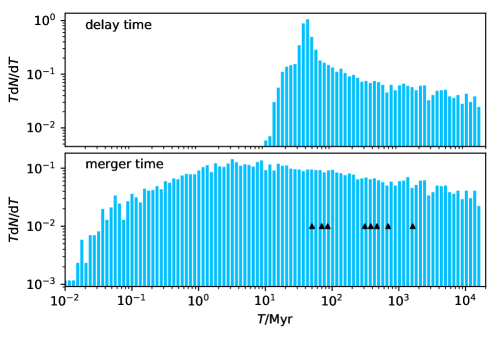
Figure 1: Merger time and delay time distributions for NS-NS systems. The eight Galactic NS-NS systems are shown with triangles.

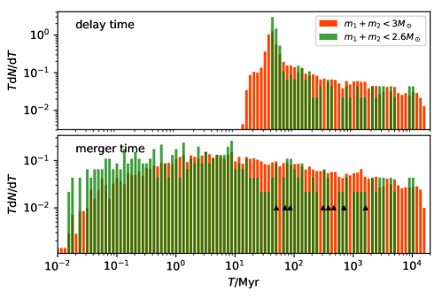
Figure 2: Merger time and delay time distribution for NS-NS systems whose mergers may produce stable NSs.

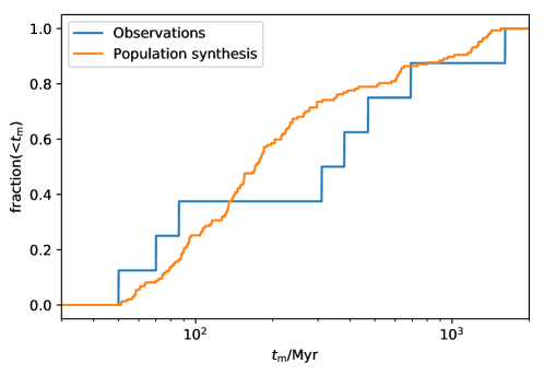
Figure 3: Cumulative distribution of merger times for NS-NS from population synthesis (orange) and observations (blue). The $p$ value is 0.22 from Kolmogorov-Smirnov test.

The delay time is defined as the time between the birth of the binary system and the final merger, while merger time refers to the time interval between the binary compact object formation and the merger. In Figure 1, we show the delay time distribution and merger time distribution for NS-NS binaries. The merger times of 8 observed field Galactic NS-NS systems (Beniamini & Piran, 2019) are shown as triangles. We also compare the cumulative distributions of merger time from population synthesis with these 8 observed field Galactic NS-NS systems. The result is shown in Figure 3. From Kolmogorov-Smirnov test, the $p$ value is 0.22, which supports that they follow the same distribution. For the delay time, as NSs’ progenitors are massive stars, their birth rate follows the star formation rate (SFR) with a minimal delay. The delay time is dominated by this gravitational wave (GW) insprial time. The time till merger depends on the initial semimajor axis $a$, and the eccentricity $e$ of the BNS as $t_{\mathrm{m}}\propto a^{4}(1-e)^{7/2}$. Under some assumptions, the delay time distribution is $\mathrm{d}N/\mathrm{d}t\propto t^{-1}$ at late times ($t\geq 1$Gyr) (Piran, 1992; Totani et al., 2008). From Figure 1, it is obvious that the merger times from population synthesis show a similar distribution. Figure 2 shows the merger time and delay time distributions for NS-NS mergers that may produce stable NSs. We can see that the distributions of delay time and merger time are almost the same in Figures 1 and 2.

3.2 Offset cumulative distribution

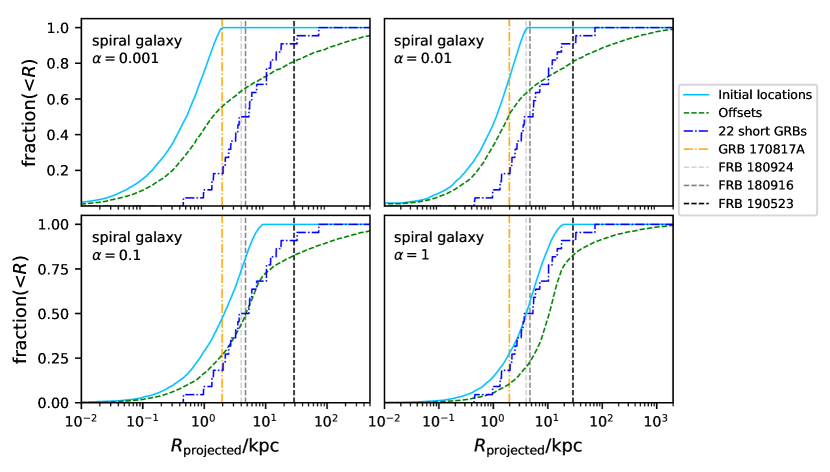
Figure 4: Initial location and offset cumulative distributions in spiral galaxies with different masses ($\alpha=0.001,0.01,0.1,1$) for NS-NS mergers. The observed offsets of 22 short GRBs, GW170817/GRB 170817A, FRB 121102, FRB 180916, FRB 180924 and FRB 190523 are also shown.

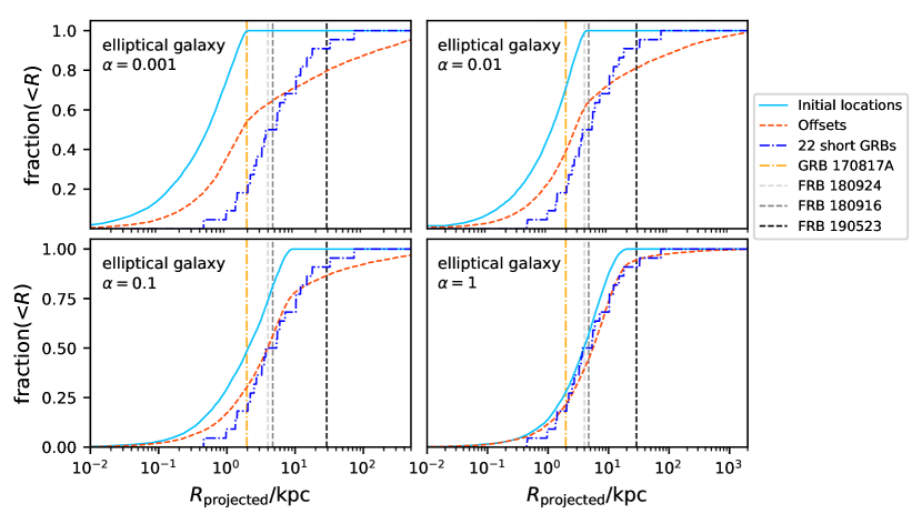
Figure 5: Initial location and offset cumulative distributions in elliptical galaxies with different masses ($\alpha=0.001,0.01,0.1,1$) for NS-NS mergers. The observed offsets of 22 short GRBs, GW170817/GRB 170817A, FRB 121102, FRB 180916, FRB 180924 and FRB 190523 are also shown.

The cumulative distributions of offsets between merger locations and centers of host galaxies for NS-NS mergers are shown in Figure 4 and Figure 5 for spiral galaxies and elliptical galaxies, respectively. The projected offset is the offset in the direction perpendicular to the line of sight. In the calculations, we average over all possible orientations of host galaxies. The observed offsets of GW170817/GRB 170817A (2 kpc) (Levan et al., 2017), FRB 180924 (4 kpc) (Bannister et al., 2019), FRB 180916 (4.7 kpc) (Marcote et al., 2020) and FRB 190523 (29 kpc) (Ravi et al., 2019) and offsets distribution of short GRBs (Fong et al., 2010, 2013; Berger, 2014) are also shown for comparison. For massive spiral galaxies ($\alpha=1$), 60% NS-NS systems will have offsets larger than 10 kpc. While for low-mass spiral galaxies ($\alpha=0.001,0.01,0.1$), the fraction is about 30%. For elliptical galaxies, the cumulative distributions of offsets are steeper when galaxy mass increases. For massive elliptical galaxies ($\alpha=0.1,1$) in Figure 5, the observed offsets of short GRBs are consistent with simulated NS-NS systems. The observed median mass of short GRBs host galaxies is about $10^{10}M_{\odot}$ (Berger, 2014), which corresponds to the $\alpha=0.1$ case.

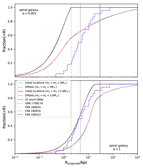
Figure 6: Initial location and offset cumulative distributions in spiral galaxies for NS-NS mergers that may produce NSs and observed offsets of short GRBs and FRBs.

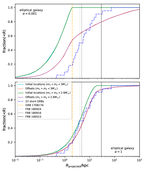
Figure 7: Initial location and offset cumulative distributions in elliptical galaxies for NS-NS mergers that may produce and observed offsets of short GRBs and FRBs.

Figures 6 and 7 show the offset distributions for NS-NS mergers that may produce NSs in spiral and elliptical galaxies respectively. For massive galaxies, the offset distributions for different upper limits of newborn NS are almost the same. For low-mass galaxies ($10^{8}M_{\odot}$), about 70% NS-NS systems will merge with offsets less than 5 kpc for $m_{1}+m_{2}\leqslant 3.0M_{\odot}$ case, while more than 80% for $m_{1}+m_{2}\leqslant 2.6M_{\odot}$ case.

3.3 Merger rate

The merger rate $R_{\mathrm{m}}(z)$ is a convolution of the star formation rate history $\rho(z)$ and the probability density function (PDF) of delay time

$$R_{\mathrm{m}}(z)=\int_{t(z)}^{t(z=\infty)}f\rho(z)\left(t^{\prime}\right)p\left[t(z)-t^{\prime}\right]\mathrm{d}t^{\prime},$$ (16)

where $\mathrm{d}t=-H(z)^{-1}(1+z)^{-1}\mathrm{d}z$, $H(z)$ is the Hubble parameter as a function of $z$, $f$ is the mass fraction of the compact binaries (NS-NS) to the entire stellar population, $t(z)$ is the cosmic age at redshift $z$. The cosmic star formation rate (CSFR) is taken from Madau & Dickinson (2014)

$$\rho(z)=0.015\frac{(1+z)^{2.7}}{1+[(1+z)/2.9]^{5.6}}M_{\odot}\text{ year }^{-1}\mathrm{Mpc}^{-3}.$$ (17)

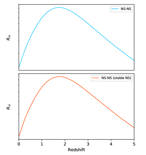
Figure 8: Merger rates $R_{\mathrm{m}}(z)$ as a function of redshift $z$ for NS-NS mergers (upper panel), and NS-NS mergers that can produce NSs (bottom panel). Rates are in arbitrary units.

When calculating the integration, we ignore the factor $f$, just showing the shape of merger rate as a function of redshift. The merger rate $R_{\mathrm{m}}(z)$ as a function of redshift $z$ are plotted in Figure 8 for $m_{1}+m_{2}\leqslant 3M_{\odot}$ before merger.

4 Local event rate

Mergers of NS-NS and NS-BH binaries have long been considered as the progenitors of short GRBs, which was confirmed by the discovery of GW170817/GRB 170817A (Abbott et al., 2017). According to GW170817, the local rate of NS-NS mergers is $\rho_{0}=1540^{+3200}_{-1220}\rm Gpc^{-3}yr^{-1}$ (Abbott et al., 2017). The local rate of short GRBs has been widely studied and found to range from several to several tens of $\rm Gpc^{-3}yr^{-1}$ (Guetta & Piran, 2006; Nakar et al., 2006; Coward et al., 2012; Wanderman & Piran, 2015; Tan et al., 2018; Zhang & Wang, 2018). According to Zhang & Wang (2018), the local rate of short GRBs is 7.53 $\rm Gpc^{-3}yr^{-1}$. If the beaming factor is chosen as $27^{+158}_{-18}$ (Fong et al., 2015), the local event rate of all short GRBs is $203_{-135}^{+1152}\rm Gpc^{-3}yr^{-1}$, which is broadly in agreement with the LIGO result.

As for the formation rate of non-repeating FRBs, we adopt the model and results given by Zhang & Wang (2019). In their calculation, considering the delay time, the cumulative redshift distribution can be derived as

$$N(<z)=T\frac{A}{4\pi}f\int_{0}^{z}\rho_{\mathrm{FRB}}(z)[\int_{0}^{1}\eta(\varepsilon)\int_{E_{t}h/\varepsilon}^{E_{max}}\Phi(E)\mathrm{d}E\mathrm{d}\varepsilon]\times\frac{\mathrm{d}V(z)}{1+z},$$ (18)

where $T$ is the observation time, $A$ is the sky area, $f_{b}$ is the beaming factor of FRB, $\Phi(E)$ is the energy distribution, $\eta(\varepsilon)$ is the beaming effect of telescope and $\rho_{FRB}(z)$ is the formation rate of FRBs. We adopt the results of Parkes with time delay (Zhang & Wang, 2019) and obtain the local formation rate as

$$\rho_{0}\simeq 6\times 10^{4}\,\bigg{(}\frac{T}{270\mathrm{s}}\bigg{)}^{-1}\bigg{(}\frac{A}{4\pi}\bigg{)}^{-1}f_{b}^{-1}\mathrm{Gpc}^{-3}\mathrm{yr}^{-1},$$ (19)

where the typical value of observation time is take from Thornton et al. (2013). This local formation rate is consistent with the result of Cao et al. (2018). It is proposed that, during the final stages of a BNS merger inspiral, the interaction between the magnetosphere could also produce a non-repeating FRB (Totani, 2013; Zhang, 2014; Wang et al., 2016; Metzger & Zivancev, 2016; Wang et al., 2018a; Zhang, 2020). However, the rate of BNS merger is well below the FRB rate, which is also discussed in Ravi (2019) for CHIME sample.

On the other hand, many bursts can be produced by the remnant NSs from BNS mergers (Yamasaki et al., 2018). If the life time of each repeater is $\tau$ years, the volume density $\rho_{\rm FRB}\tau\sim 5\times 10^{3}\,\rm{Gpc}^{-3}$ is found by Wang & Zhang (2019) above the fluence limit $F_{\rm min}=0.5$ Jy ms. The value of $\tau$ is very uncertain, which relates to the activity of newborn neutron star. The magnetic activity timescale in the direct Urca (high-mass NS) and modified Urca (normal-mass NS) case are about a few ten years and a few hundred years, respectively (Beloborodov & Li, 2016). For a lifetime of $\tau\sim(10-100)$ years, the birth rate $\rho_{\rm FRB}\sim(50-500)~{}\rm{Gpc}^{-3}yr^{-1}$ can explain the observational properties of FRB 121102, such as energy distribution (Wang & Zhang, 2019). In this case, the observed FRB rate is consistent with those of SLSNe and SGRBs (Wang & Zhang, 2019).

5 Observational properties of FRBs from BNS mergers

Most FRB models invoke coherent radiation within the magnetosphere of a magnetized neutron star (e.g. Kumar et al., 2017; Yang & Zhang, 2018; Wang & Lai, 2019). Only the fluctuation of net charges with respect to the background outflow can make a contribution to coherent radiation (Yang & Zhang, 2018). The fluctuation in the magnetosphere could be triggered by non-stationary sparks (Ruderman & Sutherland, 1975), pulsar lightning (Katz, 2017), starquake of neutron star (Wang et al., 2018b), a nearby astrophysical plasma stream (Zhang, 2017, 2018b), or exotic small bodies (Geng & Huang, 2015; Dai et al., 2016). In this section, we calculate the coherent curvature radiation by the fluctuation of the magnetosphere, and predict observation properties from the ejecta of the BNS merger.

5.1 Coherent curvature radiation by bunches

The extremely high brightness temperatures of FRBs require their radiation mechanisms to be coherent. Two coherent mechanisms are often considered in current FRB models: curvature radiation by bunches (Katz, 2014, 2018a; Kumar et al., 2017; Ghisellini & Locatelli, 2018; Yang & Zhang, 2018) and the maser mechanisms (Lyubarsky, 2014; Beloborodov, 2017; Ghisellini, 2017; Waxman, 2017; Lu & Kumar, 2018; Metzger et al., 2019). Here, we mainly consider curvature radiation by bunches as the radiation mechanism of FRBs.

First, we briefly summarize the curvature radiation by bunches following Yang & Zhang (2018). For a relativistic electron with Lorentz factor $\gamma$ moving along with a trajectory with curvature radius $\rho$, its radiation is beamed in a narrow cone of $\sim 1/\gamma$ in the electron velocity direction. In the trajectory plane, the energy radiated per unit frequency interval per unit solid angle is (Jackson, 1975)

$$\frac{\mathrm{d}I}{\mathrm{d}\omega\mathrm{d}\Omega}\simeq\frac{e^{2}}{c}\left[\frac{\Gamma(2/3)}{\pi}\right]^{2}\left(\frac{3}{4}\right)^{1/3}\left(\frac{\omega\rho}{c}\right)^{2/3}e^{-\omega/\omega_{c}},$$ (20)

where $\omega_{c}=3c\gamma^{3}/2\rho$ is the critical frequency of curvature radiation. We consider a three-dimensional bunch characterized by its length $L$, curvature radius $\rho$, bunch opening angle $\varphi$. In the bunch, the electron energy distribution is assumed to be

$$N_{e}(\gamma)\mathrm{d}\gamma=N_{e,0}(\gamma/\gamma_{m})^{-p}\mathrm{d}\gamma~{}~{}~{}{\rm for}~{}~{}~{}\gamma_{m}<\gamma<\gamma_{M}.$$ (21)

$N_{e}$ is defined as the net charge number of electrons in a bunch, considering only the net charged particles contribute to the coherent curvature radiation. Then the curvature radiation spectra are characterized by a multi-segment broken power law (see Figure 11 and Figure 12 in Yang & Zhang, 2018), with the break frequencies defined by

$$\nu_{l}=\frac{c}{\pi L},~{}~{}~{}\nu_{\varphi}=\frac{3c}{2\pi\rho\varphi^{3}}~{}~{}~{}{\rm and}~{}~{}~{}\nu_{c}=\frac{3c\gamma_{m}^{3}}{4\pi\rho}.$$ (22)

The emitted energy at the peak frequency $\nu_{\rm peak}$ is given by Yang & Zhang (2018)

$$\left.\frac{\mathrm{d}I}{\mathrm{d}\omega\mathrm{d}\Omega}\right|_{\rm peak}\simeq\frac{e^{2}}{c}K(p)N_{e,0}^{2}\gamma_{m}^{4}\left(\frac{\nu_{\rm peak}}{\nu_{c}}\right)^{2/3},$$

(23)

where $K(p)=2^{(2p-6)/3}\left[\Gamma\left(2/3\right)\Gamma\left((p-1)/3\right)\right]^{2}/3\pi^{2}$, and the peak frequency is given by $\nu_{\rm peak}=\min(\nu_{l},\nu_{\varphi},\nu_{c})$.

For a single source, e.g., a charged particle or bunch, the frequency-dependent duration of the curvature radiation is $T\sim(1-v/c)\rho/\gamma c\sim\rho/2c\gamma^{3}\sim 1/\nu_{c}$. If the electromagnetic wave frequency is considered to be $\nu_{c}\sim 10^{9}~{}{\rm Hz}$ that corresponds to the typical FRB frequency, the pulse duration of the curvature radiation will be $T\sim 1/\nu_{c}\sim 1~{}{\rm ns}$, which is much less than the observed FRB duration, $T_{\rm obs}\sim 1~{}{\rm ms}$. Therefore, there must be numerous bunches sweeping across the line of sight during the observed duration $T_{\rm obs}$ (Yang & Zhang, 2018), as shown in Figure 9. Assuming that the radiation from numerous bunches is incoherent at the observed frequency $\nu\sim 1~{}{\rm GHz}$, the observed flux density satisfies (Yang & Zhang, 2018)

$$F_{\nu}=\frac{2\pi}{TD^{2}}\frac{\mathrm{d}I}{\mathrm{d}\omega\mathrm{d}\Omega},$$ (24)

where $D$ is the source distance, and $T$ is the mean time interval between adjacent bunches. If the bunches are generated via plasma instability, the gap between adjacent bunches may be of the order of the bunch scale itself, which gives $T\sim L/c$. Thus, the observed peaked flux density is

$$F_{\nu,{\rm peak}}\simeq\frac{2\pi e^{2}}{c}K(p)\frac{N_{e,0}^{2}\gamma_{m}^{4}}{D^{2}T}\left(\frac{\nu_{\rm peak}}{\nu_{c}}\right)^{2/3}.$$ (25)

Due to $\nu_{\rm peak}\leqslant\nu_{c}$, the observed peak flux density must be less than the limit flux density

$$F_{\nu,{\rm limit}}=\frac{2\pi e^{2}}{c}K(p)\frac{N_{e,0}^{2}\gamma_{m}^{4}}{D^{2}T}.$$ (26)

5.2 FRBs from pulsar magnetosphere

As pointed out by Yang & Zhang (2018), only the fluctuation of net charges with respect to the background outflow can make a contribution to coherent radiation. We define the fraction between the fluctuating net charge density $\delta n_{\rm GJ}$ and the background Goldreich-Julian density $n_{\rm GJ}$ as

$$\mu_{c}=\frac{\delta n_{\rm GJ}}{n_{\rm GJ}},$$ (27)

one has $N_{e,{\rm tot}}=\gamma_{m}N_{e,0}/(p-1)=\mu_{c}n_{\rm GJ}V$, where $V$ is the bunch volume. When the bunches move along the field lines in the pulsar magnetosphere, the bunch opening angle $\varphi$ would depends on the magnetic field configure, as shown in Figure 9. If the emission region is close to the magnetic axis, we consider that $\varphi\sim\theta$, where $\theta$ is the polar angle. Therefore, the transverse size of a bunch is $\sim r\varphi\sim\rho\varphi^{2}$, where $r\sim\rho\theta$ is the bunch distance related to the center of magnetic dipole. The bunch volume is $V\sim L(\rho\varphi^{2})^{2}\simeq L\rho^{2}\varphi^{4}$, and one has

$$N_{e,0}=(p-1)\gamma_{m}^{-1}\mu_{c}n_{\rm GJ}L\rho^{2}\varphi^{4}$$ (28)

On the other hand, the background Goldreich-Julian density is

$$n_{\rm GJ}=\frac{B}{Pec}\left(\frac{r}{R}\right)^{-3}\sim\frac{BR^{3}}{ecP\rho^{3}\varphi^{3}},$$ (29)

where $B$ is the pulsar surface magnetic field strength, $P$ is the pulsar period, and $R$ is the pulsar radius. According to Eq.(26), Eq.(28), Eq.(29) and $T\sim L/c$, one finally has

$$F_{\nu,{\rm limit}} \simeq \frac{2\pi(p-1)^{2}K(p)}{c^{2}}\frac{\mu_{c}^{2}\gamma_{m}^{2}LB^{2}R^{6}\varphi^{2}}{D^{2}P^{2}\rho^{2}}$$ (30)

$$\simeq 3~{}{\rm Jy}\mu_{c}^{2}\gamma_{m,2}^{2}L_{1}B_{14}^{2}R_{6}^{6}\varphi_{-2}^{2}D_{\rm Gpc}^{-2}P_{-1}^{-2}\rho_{7}^{-2},$$

where the convention $Q_{x}=Q/10^{x}$ in units of cgs is adopt, $D_{\rm Gpc}=D/1~{}{\rm Gpc}$, and $(p-1)^{2}K(p)=0.4542$ for $p=3$. The intrinsic spectrum is a multi-segment broken power law with break frequencies of $\nu_{l}$, $\nu_{\varphi}$ and $\nu_{c}$ (Yang & Zhang, 2018). In the above equation, we take $L\sim 10~{}{\rm cm}$, $\varphi\sim 0.01$, $\gamma_{m}\sim 100$ and $\rho\sim 10^{7}~{}{\rm cm}$, which make $\nu_{l}\sim\nu_{\varphi}\sim\nu_{c}\simeq 1~{}{\rm GHz}$ according to Eq.(22). In this case, the spectrum above a few GHz would be very soft (with spectral index of $-(2p+4)/3$ as discussed in Yang & Zhang (2018)), which might explain the high-frequency cutoff of FRB observation. Meanwhile, if we consider that the observed narrow spectrum is due to very-soft spectrum at high frequency and radio absorption at low frequency (free-free absorption, synchrotron self-absorption, plasma absorption and etc.), the condition of the above typical frequencies at a few GHz would make the limit flux is minimum, which would gives a strongest constraint on these parameters. For an FRB with observed flux density of $F_{\nu}\sim{\rm a~{}few}~{}{\rm Jy}$, its progenitor could be a young magnetar with $B\gtrsim 10^{14}~{}{\rm G}$ and $P\lesssim 0.1~{}{\rm s}$, which could cause a large observed flux density limit $F_{\nu,{\rm limit}}$.

After the BNS merger, the newborn neutron star with a surface dipole magnetic field strength $B$ and initial period $P_{0}$ would spin down due to magnetic torques, the spindown luminosity $L_{\rm sd}$ is given by (e.g. Yang et al., 2019)

$$L_{\rm sd}=L_{\rm sd,0}\left(1+\frac{t}{t_{\rm sd}}\right)^{-2}\simeq 10^{43}~{}\mathrm{erg~{}s^{-1}}\left\{\begin{aligned} &0.4B_{14}^{-2}t_{\rm yr}^{-2}&\text{for}&~{}\text{late time}~{}t\gg t_{\rm sd}\\ &B_{12}^{2}P_{0,-3}^{-4}&\text{for}&~{}\text{early time}~{}t\ll t_{\rm sd}\\ \end{aligned}\right.$$

(31)

where $L_{\rm sd,0}=I\Omega_{0}^{2}/2t_{\rm sd}\simeq 10^{47}~{}\mathrm{erg~{}s^{-1}}B_{14}^{2}P_{0,-3}^{-4}$ is the initial spindown power, $t_{\rm sd}=3c^{3}I/B^{2}R^{6}\Omega_{0}^{2}=2\times 10^{5}~{}\mathrm{s}B_{14}^{-2}P_{0,-3}^{2}$ is the spindown timescale, $I=10^{45}~{}\mathrm{g~{}cm^{2}}$ is the moment of inertia of the neutron star, $\Omega_{0}=2\pi/P_{0}$ is the initial angular velocity of the neutron star. According to the above equation, in order to make the spindown luminosity order at the same order of magnitude as the isotropic luminosity of FRBs when an FRB occurs, for the late-time case, the neutron star is required to be a magnetar with magnetic field $B\sim 10^{14}~{}{\rm G}$, and for the early-time case, the neutron star is required to be a normal pulsar with magnetic field $B\sim 10^{2}~{}{\rm G}$. Due to the rotation energy loss, the spin period will increases with time, e.g.,

$$P=P_{0}\left(1+\frac{t}{t_{\rm sd,0}}\right)^{1/2}\simeq 1~{}{\rm ms}\left\{\begin{aligned} &12B_{14}t_{\rm yr}^{1/2}&\text{for}&~{}\text{late time}~{}t\gg t_{\rm sd}\\ &P_{0,-3}&\text{for}&~{}\text{early time}~{}t\ll t_{\rm sd}\\ \end{aligned}\right.$$

Therefore, for a magnetar with $B\sim 10^{14}~{}{\rm G}$ and $P_{0}\sim 1~{}{\rm ms}$, when its period increases to $P\lesssim 0.1~{}{\rm s}$, the magnetar age is required to be $t\lesssim 100~{}{\rm yr}$. On the other hand, if the radio bursts are powered by the rotational energy, e.g., $L_{\rm sd}\gtrsim f_{b}L_{\rm FRB}$, where $L_{\rm FRB}\sim 10^{42}~{}{\rm erg~{}s^{-1}}$ is the FRB isotropic luminosity, and $f_{b}$ is the beaming factor, the magnetar is required to be very young with

$$t<2~{}{\rm yr}f_{b}^{-1/2}L_{{\rm FRB},42}^{-1/2}B_{14}^{-1}$$ (33)

The rotational energy seems not viable as the FRB power source for a magnetar, the reason is as follows: 1. the spindown timescale of the rapidly spinning magnetar would be shorter than the observation time of FRB 121102 (Katz, 2016a, 2018b), which is of the order of several years; 2. a young ejecta associated with a magnetar with age of $t\ll 1~{}{\rm yr}$ would involve an observable DM decreasing (e.g. Piro, 2016; Yang & Zhang, 2017, see next section), which is against with the observation of FRB 121102 (Hessels et al., 2019; Josephy et al., 2019); 3. the distribution of DMs of non-repeating FRBs is inconsistent with that of expanding SNR (Katz, 2016b). Therefore, the other energy powers would be necessary, e.g., magnetic power (Metzger et al., 2017), gravitational power (Geng & Huang, 2015; Dai et al., 2016), and kinetic power (Zhang, 2017, 2018b).

5.3 Observation properties from the ejecta of binary neutron star mergers

In this section, we consider the observation properties of the ejecta of binary neutron star mergers. Different from supernova from core-collapse explosion, the ejecta by BNS merger has higher velocity $v\sim(0.1-0.3)c$ and lower mass $M\sim(10^{-4}-10^{-2})M_{\odot}$. At the time $t$ after the BNS merger, the ejecta electron density is

$$n_{e}\simeq\frac{\eta Y_{e}M}{4\pi m_{p}v^{3}t^{3}}=2.8~{}{\rm cm^{-3}}\eta Y_{e,0.2}M_{-3}v_{0.2}^{-3}t_{\rm yr}^{-3},$$ (34)

where $n_{e}$ is the free electron density, $\Delta R\sim vt$ is the ejecta thickness, $Y_{e}=0.2Y_{e,0.2}$ is the electron fraction, $\eta$ is the ionization fraction, $M_{-3}=M/10^{-3}M_{\odot}$, and $v_{0.2}=v/0.2c$. Due to $\nu_{\rm FRB}\sim 1~{}{\rm GHz}\gg\nu_{p}\simeq 10^{4}~{}{\rm Hz}\sqrt{n_{e}}\sim 17~{}{\rm kHz}$, the ejecta plasma is transparent for FRB. Besides, for an extremely young ejecta, the FRB emission may be subject to a large free-free opacity, so that the FRB may not be detected. The free-free optical depth is

$$\tau_{\rm ff}=\alpha_{\rm ff}\Delta R\simeq(0.018T_{\rm eje}^{-3/2}Z^{2}n_{e}n_{i}\nu^{-2}\bar{g}_{\rm ff})\Delta R=2.7\times 10^{-8}\eta^{2}Y_{e,0.2}^{2}M_{-3}^{2}T_{\rm eje,4}^{-3/2}\nu_{9}^{-2}v_{0.2}^{-5}t_{\rm yr}^{-5},$$ (35)

where $T_{\rm eje}=10^{4}T_{\rm eje,4}~{}{\rm K}$ is the ejecta temperature, $\bar{g}_{\rm ff}\sim 1$ is the Gaunt factor, $n_{i}$ and $n_{e}$ are the number densities of ions and electrons, respectively, and $n_{i}\sim n_{e}$ and $Z\sim 1$ are assumed in the ejecta. Thus, the ejecta will transparent for the free-free absorption a few weeks after the BNS merger.

Next, we discuss the dispersion measure and rotation measure from the ejecta. The disperse measure contributed by the ejecta is

$${\rm DM}=n_{e}\Delta R\simeq\frac{\eta Y_{e}M}{4\pi m_{p}v^{2}t^{2}}\simeq 0.17~{}{\rm pc~{}cm^{-3}}\eta Y_{e,0.2}M_{-3}v_{0.2}^{-2}t_{\rm yr}^{-2}.$$ (36)

We can see that the disperse measure contributed by the ejecta is small. Only when $t\lesssim 1~{}{\rm yr}$, the ejecta can contribute an observable DM variation. On the other hand, when the ejecta expand outward, the magnetic flux in the ejecta would keep unchanged. The total magnetic flux in the ejecta may be $\Phi\sim BR^{2}\simeq 10^{26}~{}{\rm G~{}cm^{2}}B_{14}R_{6}^{2}$. Due to the conservation of magnetic flux, one has $\Phi\sim B_{\rm eje}(vt)^{2}\sim BR^{2}$, where $B_{\rm eje}$ is the magnetic field strength in the ejecta. Finally, the RM contributed by the ejecta at time $t$ is

$$|{\rm RM}|=\frac{e^{3}B_{\rm eje}}{2\pi m_{e}^{2}c^{4}}n_{e}\Delta R\sim\frac{e^{3}}{2\pi m_{e}^{2}c^{4}}\xi BR^{2}v^{-2}t^{-2}{\rm DM}\sim 4\times 10^{-4}~{}{\rm rad~{}m^{-2}}\xi\eta Y_{e,0.2}B_{14}R_{6}^{2}M_{-3}v_{0.2}^{-4}t_{\rm yr}^{-4},$$ (37)

where the magnetic configure factor $\xi$ is defined as $\xi\equiv\left<B_{\parallel}\right>/\left<B\right>$. Notice that RM would decrease faster than DM, since the magnetic field in the ejecta also decreases with time, e.g., $B_{\rm eje}\propto t^{-2}$. In summary, for the ejecta with age of $t\gtrsim 1~{}{\rm yr}$, the corresponding ${\rm DM}$ and ${\rm RM}$ are very small.

6 Conclusions and discussion

Motivated by large offsets of FRB 180924, FRB 180916 and FRB 190523, we study FRBs from activities of NSs newborn in BNS mergers. FRB 180924 and FRB 190523 are localized to massive galaxies with low star formation rate, which are dramatically different to the host galaxy of FRB 121102. Firstly, we use the latest binary-evolution code $\mathtt{BSE}$ to calculate properties of NS-NS binaries. The merger time from population synthesis shows similar distribution as gravitational wave delay time distribution, i.e., $\mathrm{d}N/\mathrm{d}t\propto t^{-1}$ at late times. We show that the host galaxies and offsets of FRB 180924, FRB 180916 and FRB 190523 are well-matched to the distributions for NS-NS mergers from population synthesis. In addition, using the galaxy model with similar mass as short GRBs host galaxy, the offset distribution of short GRBs is well reproduced from population synthesis.

The observational properties of FRBs from BNS merger channel are also discussed. In this work, we consider that FRBs are formed by coherent curvature radiation in the magnetosphere of neutron stars (Yang & Zhang, 2018). Due to some accident events, e.g., neutron star starquake (Wang et al., 2018b), nearby astrophysical plasma (Zhang, 2017, 2018b), or exotic small bodies (Geng & Huang, 2015; Dai et al., 2016), the magnetosphere is disturbed, and the fluctuation of net charges with respect to the background Goldreich-Julian outflow would make a coherent curvature radiation. The observed flux of FRBs requires that the neutron star has large magnetic field $B\gtrsim 10^{14}~{}{\rm G}$ and fast rotation $P\lesssim 0.1~{}{\rm s}$, which corresponds to a young magnetar with age of $t\lesssim 100~{}{\rm yr}$ and the initial period of $P_{0}\sim 1~{}{\rm ms}$. Meanwhile, since the ejecta of BNS merger has high velocity $v\sim(0.1-0.3)c$ and low mass $M\sim(10^{-4}-10^{-2})M_{\odot}$, the ejecta will be transparent for free-free absorption a few weeks after the BNS merger, and the corresponding DM and RM are very small for the ejecta with age of $t\gtrsim 1~{}{\rm yr}$.

In the BNS merger scenario, it would be possible that we observe associations of FRBs with short GRBs and gravitational wave (GW) events. In the future, if more FRBs are localized, the offset distribution of short GRBs can be compared with that of FRBs. Since the magnetar born in BNS merger can show magnetic activity for a long time (Beloborodov & Li, 2016; Beloborodov, 2019), we can search FRBs in the location region of short GRBs and BNS merger GW events.

Figure 9: A cartoon figure for coherent curvature radiation by bunches in magnetosphere. The gray dark regions denote the bunches which are generated by the fluctuation of net charges with respect to the Goldreich-Julian background outflow. $L$ is the bunch length, and $\varphi$ is the bunch opening angle.

References

- Aarseth (2012) Aarseth, S. J. 2012, MNRAS, 422, 841
- Abbott et al. (2017) Abbott, B. P., Abbott, R., Abbott, T. D., et al. 2017, Physical Review Letters, 119, 161101
- Bajkova & Bobylev (2017) Bajkova, A., & Bobylev, V. 2017, Open Astronomy, 26, 72
- Banerjee et al. (2019) Banerjee, S., Belczynski, K., Fryer, C. L., et al. 2019, arXiv e-prints, arXiv:1902.07718
- Bannister et al. (2019) Bannister, K. W., Deller, A. T., Phillips, C., et al. 2019, Science, 365, 565
- Barthelmy et al. (2005) Barthelmy, S. D., Chincarini, G., Burrows, D. N., et al. 2005, Nature, 438, 994
- Belczynski et al. (2010) Belczynski, K., Bulik, T., Fryer, C. L., et al. 2010, ApJ, 714, 1217
- Belczynski et al. (2002) Belczynski, K., Bulik, T., & Rudak, B. 2002, ApJ, 571, 394
- Belczynski et al. (2008) Belczynski, K., Kalogera, V., Rasio, F. A., et al. 2008, ApJS, 174, 223
- Belczynski et al. (2006) Belczynski, K., Perna, R., Bulik, T., et al. 2006, ApJ, 648, 1110
- Belczynski et al. (2016) Belczynski, K., Heger, A., Gladysz, W., et al. 2016, A&A, 594, A97
- Beloborodov (2017) Beloborodov, A. M. 2017, ApJ, 843, L26
- Beloborodov (2019) —. 2019, arXiv e-prints, arXiv:1908.07743
- Beloborodov & Li (2016) Beloborodov, A. M., & Li, X. 2016, ApJ, 833, 261
- Beniamini & Piran (2019) Beniamini, P., & Piran, T. 2019, MNRAS, 487, 4847
- Berger (2014) Berger, E. 2014, ARA&A, 52, 43
- Bethe & Brown (1998) Bethe, H. A., & Brown, G. E. 1998, ApJ, 506, 780
- Bloom et al. (1999) Bloom, J. S., Sigurdsson, S., & Pols, O. R. 1999, MNRAS, 305, 763
- Bloom et al. (2006) Bloom, J. S., Prochaska, J. X., Pooley, D., et al. 2006, ApJ, 638, 354
- Cao et al. (2018) Cao, X.-F., Yu, Y.-W., & Zhou, X. 2018, ApJ, 858, 89
- Champion et al. (2016) Champion, D. J., Petroff, E., Kramer, M., et al. 2016, MNRAS, 460, L30
- Chatterjee et al. (2017) Chatterjee, S., Law, C. J., Wharton, R. S., et al. 2017, Nature, 541, 58
- Cheng et al. (2020) Cheng, Y., Zhang, G. Q., & Wang, F. Y. 2020, MNRAS, 491, 1498
- Cordes & Chatterjee (2019) Cordes, J. M., & Chatterjee, S. 2019, ARA&A, 57, 417
- Cordes et al. (2017) Cordes, J. M., Wasserman, I., Hessels, J. W. T., et al. 2017, ApJ, 842, 35
- Coward et al. (2012) Coward, D. M., Howell, E. J., Piran, T., et al. 2012, MNRAS, 425, 2668
- Dai et al. (2016) Dai, Z. G., Wang, J. S., Wu, X. F., & Huang, Y. F. 2016, ApJ, 829, 27
- Dai et al. (2006) Dai, Z. G., Wang, X. Y., Wu, X. F., & Zhang, B. 2006, Science, 311, 1127
- de Mink & Belczynski (2015) de Mink, S. E., & Belczynski, K. 2015, ApJ, 814, 58
- Duquennoy & Mayor (1991) Duquennoy, A., & Mayor, M. 1991, A&A, 500, 337
- Fong et al. (2010) Fong, W., Berger, E., & Fox, D. B. 2010, ApJ, 708, 9
- Fong et al. (2015) Fong, W., Berger, E., Margutti, R., & Zauderer, B. A. 2015, ApJ, 815, 102
- Fong et al. (2013) Fong, W., Berger, E., Chornock, R., et al. 2013, ApJ, 769, 56
- Fox et al. (2005) Fox, D. B., Frail, D. A., Price, P. A., et al. 2005, Nature, 437, 845
- Fryer et al. (2012) Fryer, C. L., Belczynski, K., Wiktorowicz, G., et al. 2012, ApJ, 749, 91
- Fryer et al. (1999) Fryer, C. L., Woosley, S. E., & Hartmann, D. H. 1999, ApJ, 526, 152
- Gao et al. (2014) Gao, H., Li, Z., & Zhang, B. 2014, ApJ, 788, 189
- Gehrels et al. (2005) Gehrels, N., Sarazin, C. L., O’Brien, P. T., et al. 2005, Nature, 437, 851
- Geng & Huang (2015) Geng, J. J., & Huang, Y. F. 2015, ApJ, 809, 24
- Ghisellini (2017) Ghisellini, G. 2017, MNRAS, 465, L30
- Ghisellini & Locatelli (2018) Ghisellini, G., & Locatelli, N. 2018, A&A, 613, A61
- Guetta & Piran (2006) Guetta, D., & Piran, T. 2006, A&A, 453, 823
- Hansen & Phinney (1997) Hansen, B. M. S., & Phinney, E. S. 1997, MNRAS, 291, 569
- Hernquist (1990) Hernquist, L. 1990, ApJ, 356, 359
- Hessels et al. (2019) Hessels, J. W. T., Spitler, L. G., Seymour, A. D., et al. 2019, ApJ, 876, L23
- Hurley et al. (2002) Hurley, J. R., Tout, C. A., & Pols, O. R. 2002, MNRAS, 329, 897
- Jackson (1975) Jackson, J. D. 1975, Classical electrodynamics
- Josephy et al. (2019) Josephy, A., Chawla, P., Fonseca, E., et al. 2019, ApJ, 882, L18
- Katz (1975) Katz, J. I. 1975, Nature, 253, 698
- Katz (2014) —. 2014, Phys. Rev. D, 89, 103009
- Katz (2016a) —. 2016a, Modern Physics Letters A, 31, 1630013
- Katz (2016b) —. 2016b, ApJ, 826, 226
- Katz (2017) —. 2017, MNRAS, 469, L39
- Katz (2018a) —. 2018a, MNRAS, 481, 2946
- Katz (2018b) —. 2018b, Progress in Particle and Nuclear Physics, 103, 1
- Kulkarni et al. (2014) Kulkarni, S. R., Ofek, E. O., Neill, J. D., Zheng, Z., & Juric, M. 2014, ApJ, 797, 70
- Kumar et al. (2017) Kumar, P., Lu, W., & Bhattacharya, M. 2017, MNRAS, 468, 2726
- Levan et al. (2017) Levan, A. J., Lyman, J. D., Tanvir, N. R., et al. 2017, ApJ, 848, L28
- Li et al. (2019a) Li, Y., Zhang, B., Nagamine, K., & Shi, J. 2019a, ApJ, 884, L26
- Li et al. (2019b) Li, Z., Gao, H., Wei, J.-J., et al. 2019b, ApJ, 876, 146
- Li et al. (2018) Li, Z.-X., Gao, H., Ding, X.-H., Wang, G.-J., & Zhang, B. 2018, Nature Communications, 9, 3833
- Liu et al. (2019) Liu, B., Li, Z., Gao, H., & Zhu, Z.-H. 2019, Physical Review D, 99, 123517
- Lorimer et al. (2007) Lorimer, D. R., Bailes, M., McLaughlin, M. A., Narkevic, D. J., & Crawford, F. 2007, Science, 318, 777
- Lü et al. (2015) Lü, H.-J., Zhang, B., Lei, W.-H., Li, Y., & Lasky, P. D. 2015, ApJ, 805, 89
- Lu & Kumar (2016) Lu, W., & Kumar, P. 2016, MNRAS, 461, L122
- Lu & Kumar (2018) —. 2018, MNRAS, 477, 2470
- Lyubarsky (2014) Lyubarsky, Y. 2014, MNRAS, 442, L9
- Madau & Dickinson (2014) Madau, P., & Dickinson, M. 2014, ARA&A, 52, 415
- Marcote et al. (2017) Marcote, B., Paragi, Z., Hessels, J. W. T., et al. 2017, ApJ, 834, L8
- Marcote et al. (2020) Marcote, B., Nimmo, K., Hessels, J. W. T., et al. 2020, Nature, 577, 190
- Margalit et al. (2019) Margalit, B., Berger, E., & Metzger, B. D. 2019, ApJ, 886, 110
- Metzger et al. (2017) Metzger, B. D., Berger, E., & Margalit, B. 2017, ApJ, 841, 14
- Metzger et al. (2019) Metzger, B. D., Margalit, B., & Sironi, L. 2019, MNRAS, 485, 4091
- Metzger et al. (2008) Metzger, B. D., Quataert, E., & Thompson, T. A. 2008, MNRAS, 385, 1455
- Metzger & Zivancev (2016) Metzger, B. D., & Zivancev, C. 2016, MNRAS, 461, 4435
- Miyamoto & Nagai (1975) Miyamoto, M., & Nagai, R. 1975, PASJ, 27, 533
- Murase et al. (2016) Murase, K., Kashiyama, K., & Mészáros, P. 2016, MNRAS, 461, 1498
- Nakar et al. (2006) Nakar, E., Gal-Yam, A., & Fox, D. B. 2006, ApJ, 650, 281
- Navarro et al. (1996) Navarro, J. F., Frenk, C. S., & White, S. D. M. 1996, ApJ, 462, 563
- Nicholl et al. (2017) Nicholl, M., Williams, P. K. G., Berger, E., et al. 2017, ApJ, 843, 84
- Paczynski (1990) Paczynski, B. 1990, ApJ, 348, 485
- Perna & Belczynski (2002) Perna, R., & Belczynski, K. 2002, ApJ, 570, 252
- Petroff et al. (2019) Petroff, E., Hessels, J. W. T., & Lorimer, D. R. 2019, A&A Rev., 27, 4
- Piran (1992) Piran, T. 1992, ApJ, 389, L45
- Piro (2016) Piro, A. L. 2016, ApJ, 824, L32
- Platts et al. (2019) Platts, E., Weltman, A., Walters, A., et al. 2019, Phys. Rep., 821, 1
- Podsiadlowski et al. (2004) Podsiadlowski, P., Langer, N., Poelarends, A. J. T., et al. 2004, ApJ, 612, 1044
- Popov & Postnov (2013) Popov, S. B., & Postnov, K. A. 2013, arXiv e-prints, arXiv:1307.4924
- Ravi (2019) Ravi, V. 2019, Nature Astronomy, 405
- Ravi et al. (2019) Ravi, V., Catha, M., D’Addario, L., et al. 2019, arXiv e-prints, arXiv:1907.01542
- Rowlinson et al. (2013) Rowlinson, A., O’Brien, P. T., Metzger, B. D., Tanvir, N. R., & Levan, A. J. 2013, MNRAS, 430, 1061
- Ruderman & Sutherland (1975) Ruderman, M. A., & Sutherland, P. G. 1975, ApJ, 196, 51
- Sana et al. (2012) Sana, H., de Mink, S. E., de Koter, A., et al. 2012, Science, 337, 444
- Scalo (1986) Scalo, J. M. 1986, Fund. Cosmic Phys., 11, 1
- Shannon et al. (2018) Shannon, R. M., Macquart, J. P., Bannister, K. W., et al. 2018, Nature, 562, 386
- Tan et al. (2018) Tan, W.-W., Fan, X.-L., & Wang, F. Y. 2018, MNRAS, 475, 1331
- Tendulkar et al. (2017) Tendulkar, S. P., Bassa, C. G., Cordes, J. M., et al. 2017, ApJ, 834, L7
- Thornton et al. (2013) Thornton, D., Stappers, B., Bailes, M., et al. 2013, Science, 341, 53
- Totani (2013) Totani, T. 2013, PASJ, 65, L12
- Totani et al. (2008) Totani, T., Morokuma, T., Oda, T., Doi, M., & Yasuda, N. 2008, PASJ, 60, 1327
- Voss & Tauris (2003) Voss, R., & Tauris, T. M. 2003, MNRAS, 342, 1169
- Walters et al. (2018) Walters, A., Weltman, A., Gaensler, B. M., Ma, Y.-Z., & Witzemann, A. 2018, ApJ, 856, 65
- Wanderman & Piran (2015) Wanderman, D., & Piran, T. 2015, MNRAS, 448, 3026
- Wang & Dai (2013) Wang, F. Y., & Dai, Z. G. 2013, Nature Physics, 9, 465
- Wang & Yu (2017) Wang, F. Y., & Yu, H. 2017, J. Cosmology Astropart. Phys, 03, 023
- Wang & Zhang (2019) Wang, F. Y., & Zhang, G. Q. 2019, ApJ, 882, 108
- Wang & Lai (2019) Wang, J.-S., & Lai, D. 2019, arXiv e-prints, arXiv:1907.12473
- Wang et al. (2018a) Wang, J.-S., Peng, F.-K., Wu, K., & Dai, Z.-G. 2018a, The Astrophysical Journal, 868, 19
- Wang et al. (2016) Wang, J.-S., Yang, Y.-P., Wu, X.-F., Dai, Z.-G., & Wang, F.-Y. 2016, ApJ, 822, L7
- Wang et al. (2018b) Wang, W., Luo, R., Yue, H., et al. 2018b, ApJ, 852, 140
- Wang & Wang (2018) Wang, Y. K., & Wang, F. Y. 2018, A&A, 614, A50
- Waxman (2017) Waxman, E. 2017, ApJ, 842, 34
- Wei et al. (2015) Wei, J.-J., Gao, H., Wu, X.-F., & Mészáros, P. 2015, Phys. Rev. Lett., 115, 261101
- Yamasaki et al. (2018) Yamasaki, S., Totani, T., & Kiuchi, K. 2018, PASJ, 70, 39
- Yang & Zhang (2016) Yang, Y.-P., & Zhang, B. 2016, ApJ, 830, L31
- Yang & Zhang (2017) —. 2017, ApJ, 847, 22
- Yang & Zhang (2018) —. 2018, ApJ, 868, 31
- Yang et al. (2019) Yang, Y.-P., Zhang, B., & Wei, J.-Y. 2019, ApJ, 878, 89
- Yu & Wang (2017) Yu, H., & Wang, F. Y. 2017, A&A, 606, A3
- Yu & Wang (2018) —. 2018, European Physical Journal C, 78, 692
- Zhang (2014) Zhang, B. 2014, ApJ, 780, L21
- Zhang (2017) —. 2017, ApJ, 836, L32
- Zhang (2018a) —. 2018a, ApJ, 867, L21
- Zhang (2018b) —. 2018b, ApJ, 854, L21
- Zhang (2020) —. 2020, arXiv e-prints, arXiv:2002.00335
- Zhang & Wang (2018) Zhang, G. Q., & Wang, F. Y. 2018, ApJ, 852, 1
- Zhang & Wang (2019) —. 2019, MNRAS, 487, 3672
- Zhou et al. (2014) Zhou, B., Li, X., Wang, T., Fan, Y.-Z., & Wei, D.-M. 2014, Phys. Rev. D, 89, 107303