Regularized Submodular Maximization at Scale

Abstract

In this paper, we propose scalable methods for maximizing a regularized submodular function $f(\cdot)=g(\cdot)-\ell(\cdot)$ expressed as the difference between a monotone submodular function $g$ and a modular function $\ell$. Indeed, submodularity is inherently related to the notions of diversity, coverage, and representativeness. In particular, finding the mode (i.e., the most likely configuration) of many popular probabilistic models of diversity, such as determinantal point processes, submodular probabilistic models, and strongly log-concave distributions, involves maximization of (regularized) submodular functions. Since a regularized function $f$ can potentially take on negative values, the classic theory of submodular maximization, which heavily relies on the assumption that the submodular function is non-negative, may not be applicable. To circumvent this challenge, we develop Distorted-Streaming, the first one-pass streaming algorithm for maximizing a regularized submodular function subject to a $k$-cardinality constraint. It returns a solution $S$ with the guarantee that $f(S)\geq(\phi^{-2}-\varepsilon)\cdot g(OPT)-\ell(OPT)$, where $\phi$ is the golden ratio (and thus, $\phi^{-2}\approx 0.382$). Furthermore, we develop Distorted-Distributed-Greedy, the first distributed algorithm that returns a solution $S$ with the guarantee that $\bE[f(S)]\geq(1-\varepsilon)\left[(1-e^{-1})\cdot g(OPT)-\ell(OPT)\right]$ in $O(1/\varepsilon)$ rounds of MapReduce computation. We should highlight that our result, even for the unregularized case where the modular term $\ell$ is zero, improves the memory and communication complexity of the existing work by a factor of $O(1/\varepsilon)$ as it manages to avoid the need (of this existing work) to keep multiple copies of the entire dataset. Moreover, it does so while (arguably) providing a simpler distributed algorithm and a unifying analysis. We also empirically study the performance of our scalable methods on a set of real-life applications, including vertex cover of social networks, mode of strongly log-concave distributions, data summarization (such as video summarization, location summarization, and text summarization), and product recommendation.

1 Introduction

Finding a diverse set of items, also known as data summarization, is one of the central tasks in machine learning. It usually involves either maximizing a utility function that promotes coverage and representativeness [44, 58] (we call this an optimization perspective) or sampling from discrete probabilistic models that promote negative correlations and show repulsive behaviors [52, 24] (we call this a sampling perspective). Celebrated examples of probabilistic models that encourage negative dependency include determinantal point processes [35], strongly Rayleigh measures [6] strongly log-concave distributions [25], and probabilistic submodular models [13, 30]. In fact, the two above views are tightly related in the sense that oftentimes the mode (i.e., most likely configuration) of a diversity promoting distribution is a simple variant of a (regularized) submodular function. For instance, determinantal point processes are log-submodular. Or, as we show later, a strongly log-concave distribution is indeed a regularized log-submodular plus a log quadratic term. The aim of this paper is to show how such an optimization task can be done at scale.

From the optimization perspective, in order to effectively select a diverse subset of items, we need to define a measure that captures the amount of representativeness that lies within a selected subset. Oftentimes, such a measure naturally satisfies the intuitive diminishing returns condition which can be formally captured by submodularity. Given a finite ground set $\cN$ of size $n$, consider a set function $g\colon 2^{\cN}\to\bR$ assigning a utility $g(A)$ to every subset $A\subseteq\cN$. We say that $g$ is submodular if for any pair of subsets $A\subseteq B\subseteq\operatorname{\cN}$ and an element $u\not\in B$, we have $g(A\cup\{u\})-g(A)\geq g(B\cup\{u\})-g(B),$ which intuitively means that the increase in “representativeness” following the addition of an element $u$ is smaller when $u$ is added to a larger set. Additionally, a set function is said to be monotone if $g(A)\leq g(B)$ for all $A\subseteq B\subseteq\cN$; that is, adding more data can only increase the representativeness of any subset. Many of the previous work in data summarization and diverse subset selection that take an optimization perspective, simply aim to maximize a monotone submodular function [44]. Monotonicity has the advantage of promoting coverage, but it also enhances the danger of over-fitting to the data as adding more elements can never decrease the utility. To address this issue, as it is often done in machine learning, we need to add a simple penalty or a regularizer term. Formally, we cast this optimization problem as an instance of regularized submodular maximization, in which we are asked to find a set $S$ of size at most $k$ that maximizes

$$OPT=\operatorname*{arg\,max}_{S\subseteq\cN,|S|\leq k}[g(S)-\ell(S)]\enspace,$$ (1)

where $g$ is a non-negative monotone submodular function and $\ell$ is a non-negative modular function. The role of the modular function $\ell$ is to discount the benefit of adding elements. We highlight that $g-\ell$ is still submodular. However, it may no longer be non-negative, an assumption that is essential for deriving competitive algorithms with constant-factor approximation guarantees (for more information, see the survey by [7]). Even though maximizing a regularized submodular function has been proposed in the past as a more faithful model of diverse data selection [57], formal treatment of this problem has only recently been done [55, 18, 28].

In many practical scenarios, random access to the entire data is not possible and only a small fraction of the data can be loaded to the main memory, there is only time to read the data once, and the data arrives at a very fast pace. Furthermore, the amount of collected data is often too large to solve the optimization problem on a single machine. Prior to this work, no streaming or distributed algorithm to solve Problem (1) was established. However, based on ideas from [55, 18], Harshaw et al. [28] proposed Distorted-Greedy, an efficient offline algorithm to (approximately) solve this problem. This algorithm iteratively and greedily finds elements that maximize a distorted function. On the other hand, Distorted-Greedy, as a centralized algorithm, requires a memory that grows linearly with the size of the data, and it needs to make multiple passes ($\Theta(n)$ in the worst case) over the data; therefore it fails to satisfy the above mentioned requirements of modern applications. Indeed, with the unprecedented increase in the data size in recent years, scalable data summarization has gained a lot of attention with far-reaching applications, including brain parcellation from fMRI data [54], interpreting neural networks [14], selecting panels of genomics assays [59], video [26], image [56, 57], and text [39, 33] summarization, and sparse feature selections [15, 11], to name a few. In this paper, we propose scalable methods (in both streaming and distributed settings) for maximizing a regularized submodular function. In the following, we briefly explain our main theoretical results. Our Results. In Section 3, we introduce Distorted-Streaming, the first one-pass streaming algorithm for maximizing a regularized submodular function subject to a $k$-cardinality constraint. Theorem 1 guarantees the performance of Threshold-Streaming.

Theorem 1.

For every $\varepsilon,r>0$, Threshold-Streaming produces a set $S\subseteq\cN$ of size at most $k$ for Problem (1), obeying $g(S)-\ell(S)\geq\max_{T\subseteq\cN,|T|\leq k}[(h(r)-\varepsilon)\cdot g(T)-r\cdot\ell(T)]$, where $h(r)=\frac{2r+1-\sqrt{4r^{2}+1}}{2}$.

We should point out that previous studies of Problem (1), for various theoretical and practical reasons, have only focused on the case in which $r=1$ and $T$ is the set $OPT$ of size at most $k$ maximizing $g(T)-\ell(T)$ [55, 18, 28]. In this case, we get the following corollary from the result of Theorem 1.

Corollary 2.

For every $\varepsilon>0$, Threshold-Streaming produces a set $S\subseteq\cN$ of size at most $k$ for Problem (1) obeying $g(S)-\ell(S)\geq(\phi^{-2}-\varepsilon)\cdot g(OPT)-\ell(OPT)$, where $\phi$ is the golden ratio (and thus, $\phi^{-2}\approx 0.382$).

In Section 4, we develop Distorted-Distributed-Greedy, the first distributed algorithm for regularized submodular maximization in a MapReduce model of computation. This algorithm allows us to distribute data across several machines and use their combined computational resources. Interestingly, even for the classic case of an unregulated monotone submodular function, our distributed algorithm improves over space and communication complexity of the existing work [5] by a factor of $\Theta(1/\varepsilon)$. The approximation guarantee of Distorted-Distributed-Greedy is given in Theorem 3.

Theorem 3.

Distorted-Distributed-Greedy (Algorithm 3) returns a set $D\subseteq\cN$ of size at most $k$ such that

$$\frac{\bE[g(D)-\ell(D)]}{1-\varepsilon}\geq(1-e^{-1})\cdot g(OPT)-\ell(OPT).$$

Finally, as our algorithms can efficiently find diverse elements from massive datasets, in Sections 5 and 6, we explore the power of the regularized submodular maximization approach and our algorithms in several real-world applications through an extensive set of experiments.

2 Related Work

Finding the optimal solution for a submodular maximization problem is computationally hard even in the absence of a constraint [17]. Nevertheless, the well-known result of Nemhauser et al. [50] showed that the classical greedy algorithm obtains a $(1-1/e)$-approximation for maximizing a non-negative and monotone submodular function subject to a cardinality constraint, which is known to be optimal [49]. However, when the objective function is non-monotone or the constraint is more complex, the vanilla greedy algorithm may perform much worse. An extensive line of research has lead to the development of algorithms for handling non-monotone submodular objectives subject to more complicated constraints (see, e.g., [37, 19, 2, 45, 20]). We should note that, up until very recently, all the existing works required the objective function to take only non-negative values, an assumption that may not hold in many applications [28].

The first work to handle submodular objective functions that might take negative values is the work of Sviridenko et al. [55], which studies the maximization of submodular function that can be decomposed as a sum $g+c$, where $g$ is a non-negative monotone submodular function and $c$ is an (arbitrary) modular function. For this problem, Sviridenko et al. [55] gave two randomized polynomial-time algorithms which produce a set $S$ that roughly obeys $g(S)+c(S)\geq(1-1/e)\cdot g(OPT)+c(OPT)$, where $OPT$ is the optimal set. Both algorithms of Sviridenko et al. [55] are mainly of theoretical interest, as their computational complexity is quite prohibitive. Feldman [18] reconsidered one of these algorithms, and showed that one of the costly steps in it (namely, a step in which the algorithm guesses the value of $c(OPT)$) can be avoided using a surrogate objective that varies with time. Nevertheless, the algorithm of [18] remains quite involved as it optimizes a fractional version of the problem—which is necessary for allowing it to handle various kinds of complex constraints. Harshaw et al. [28] showed that in the case of a cardinality constraint (and a non-negative $c$) much of this complexity can be avoided, yielding the first practical algorithm Distorted-Greedy. They also extended their results to $\gamma$-weakly submodular functions and the unconstrained setting.

Due to the massive volume of the current data sets, scalable methods have gained a lot of interest in machine learning applications. One appealing approach towards this goal is to design streaming algorithms. Badanidiyuru et al. [3] were the first to consider a single-pass streaming algorithm for maximizing a monotone submodular function under a cardinality constraint. Their result was later improved and extended to non-monotone functions [1, 16, 32] and subject to more involved constraints [8, 9, 10, 21]. Another scalable approach is the development of distributed algorithms through the MapReduce framework where the data is split amongst several machines and processed in parallel [36, 46, 4, 43, 5, 41].

In the context of discrete probabilistic models, it is well-known that strongly Rayleigh (SR) measures [6] (including determinantal point processes [35]) or the more general class of strongly log-concave (SLC) distributions [25] provide strong negative dependence among sampling items. Although Gotovos [23] recently showed that strong log-concavity does not imply log-submodularity, Robinson et al. [53] argued that the logarithm of an SLC distribution enjoys a variant of approximate submodularity. We build on this result and derive a slight improvement, along with corresponding guarantees for streaming and distributed solutions.

3 Streaming Algorithm

In this section, we present our proposed streaming algorithm for Problem (1). To explain our algorithm, let us first define $T$ to be a subset of $\cN$ of size at most $k$ such that

$$T\in\operatorname*{arg\,max}_{S\subseteq\cN,|S|\leq k}[(h(r)-\varepsilon)\cdot g(T)-r\cdot\ell(T)]\enspace,$$

where $r$ is some positive real value to be discussed later, and $h(r)=\frac{2r+1-\sqrt{4r^{2}+1}}{2}$. A basic version of our proposed algorithm, named Threshold-Streaming, is given as Algorithm 1. We note that this algorithm guesses, in the first step, a value $\tau>0$ which obeys $k\tau\leq h(r)\cdot g(T)-r\cdot\ell(T)\leq(1+\varepsilon)k\tau$. In Algorithm 1, to avoid unnecessary technicalities, we simply assume that the algorithm can guess such a value for $\tau$ based on some oracle. In Appendix A, we explain how a technique from [3] can be used for that purpose at the cost of increasing the space complexity of the algorithm by a factor of $O(\varepsilon^{-1}(\log k+\log r^{-1}))$. Algorithm 1 starts with an empty set $S$. While the data stream is not empty yet and the size of set $S$ is still smaller than $k$, for every incoming element $u$, the value of $g(u\mid S)-\alpha(r)\cdot\ell(\{u\})$ is calculated, where we define $\alpha(r)=\frac{2r+1+\sqrt{4r^{2}+1}}{2}$. If this value is at least $\tau$, then $u$ is added to $S$ by the algorithm. The theoretical guarantee of Algorithm 1 is provided in Theorem 1, and the proof of this theorem is given in Section 3.2.

1 Guess a value $\tau$ such that $k\tau\leq h(r)\cdot g(T)-r\cdot\ell(T)\leq(1+\varepsilon)k\tau$.

2 Let $\alpha(r)\leftarrow\frac{2r+1+\sqrt{4r^{2}+1}}{2}$.

3 Let $S\leftarrow\varnothing$.

4 while $|S|<k$ and there are more elements do

5       Let $u$ be the next elements in the stream.

6       if $g(u\mid S)-\alpha(r)\cdot\ell(\{u\})\geq\tau$ then

7             Add $u$ to the set $S$.

8      

return the better solution among $S$ and $\varnothing$.

Algorithm 1 Threshold-Streaming

3.1 How to Choose a Good Value of $r$?

In this section, we study the effect of the parameter $r$ on the performance of Algorithm 1 under different settings. First note that the bound given by Corollary 2 reduces to a trivial lower bound of $0$ when $\phi^{-2}\cdot g(OPT)\leq\ell(OPT)$. A similar phenomenon happens for the bound of [28, Theorem 3] when $(1-e^{-1})\cdot g(OPT)\leq\ell(OPT)$. Namely, in this regimen their bound (i.e., $(1-e^{-1})\cdot g(OPT)-\ell(OPT)$) becomes trivial. We now explain how a carefully chosen value for $r$ can be used to prevent this issue.

For a set $S$, let $\beta_{S}$ denote the ratio between the utility of $S$ and its linear cost, i.e., $\beta_{S}=\frac{g(S)-\ell(S)}{\ell(S)}$. Using this terminology, we get that the guarantees of Corollary (2) and [28, Theorem 3] become trivial when $\beta_{OPT}\leq\phi^{2}-1=\phi$ and $\beta_{OPT}\leq\nicefrac{{1}}{{(e-1)}}$, respectively. In Corollary 4, we show that by knowing the value of $\beta_{OPT}$ we can find a value for $r$ in Algorithm 1 which makes Theorem 1 yield the strongest guarantee for (1), and moreover, this guarantee is non-trivial as long as $\beta_{OPT}>0$ (if $\beta_{OPT}\leq 0$, then the empty set is a trivial optimal solution).

Corollary 4.

Assume the value of $\beta_{OPT}$ is given, where $OPT$ is the optimal solution of Problem (1). Setting $r=r_{OPT}=\frac{\beta_{OPT}}{2\sqrt{1+2\beta_{OPT}}}$ makes Algorithm 1 return a solution $S$ with the guarantee

$$g(S)-\ell(S)\geq\left(\frac{1+\beta_{OPT}-\sqrt{1+2\beta_{OPT}}}{2\beta_{OPT}}-\varepsilon^{\prime}\right)\cdot(g(OPT)-\ell(OPT))\enspace,$$

where $\varepsilon^{\prime}=\varepsilon\cdot(1+1/\beta_{OPT})$.

Proof.

First, let us define $T^{*}_{r}=\operatorname*{arg\,max}_{T\in\cN,|T|\leq k}[(h(r)-\varepsilon)\cdot g(T)-r\cdot\ell(T)]$. From Theorem 1 and the definition of $T^{*}_{r}$, we have

$$g(S)-\ell(S)\geq(h(r)-\varepsilon)\cdot g(T^{*}_{r})-r\cdot\ell(T^{*})\geq(h(r)-\varepsilon)\cdot g(OPT)-r\cdot\ell(OPT)\enspace.$$

Furthermore, from the definition of $\beta_{OPT}$, we have

$$(h(r)-\varepsilon)\cdot g(OPT)-r\cdot\ell(OPT)={} \frac{(h(r)-\varepsilon)\cdot g(OPT)-r\cdot\ell(OPT)}{g(OPT)-\ell(OPT)}\cdot(g(OPT)-\ell(OPT))$$

$$={} \frac{(h(r)-\varepsilon)\cdot(1+\beta_{OPT})-r}{\beta_{OPT}}\cdot(g(OPT)-\ell(OPT))\enspace.$$

It can be verified that $r_{OPT}$ is the value that maximizes the above expression, and plugging this value into the expression proves the corollary. ∎

From the definition of $\beta_{OPT}$, it can be observed that for larger values of $\beta_{OPT}$ the effect of the modular cost function over the utility diminishes and $g-\ell$ gets closer to a monotone and non-negative submodular function. At the same time, from Corollary 4 we see that for large values of $\beta_{OPT}$ the approximation factor approaches $\nicefrac{{1}}{{2}}$. Norouzi-Fard et al. [51] gave evidence that the last approximation ratio is optimal when the objective function is indeed non-negative and monotone, which could be an indicator for the optimality of our streaming algorithm for (1). Indeed, we conjecture that Threshold-Streaming, when choosing $r$ based on $\beta_{OPT}$ as in Corollary 4, achieves the best possible guarantee for Problem (1) in the streaming setting.

In order to apply the result of Corollary 4 to obtain the strongest guarantee for Problem (1), we need to have access to the set $OPT$ (and consequently $\beta_{OPT}$ and $r_{OPT}$); but, unfortunately, none of these is known a priori. Next, we propose an efficient approach that enables us to find an accurate enough estimate of $r_{OPT}$. Let $\zeta_{OPT}=\frac{1+\beta_{OPT}-\sqrt{1+2\beta_{OPT}}}{2\beta_{OPT}}$ be the approximation ratio that can be obtained for the unknown value of $\beta_{OPT}$ via Corollary 4 (except for the $\varepsilon^{\prime}$ error term). This definition implies that we always have $0\leq\zeta_{OPT}<\nicefrac{{1}}{{2}}$. Thus, we can find an accurate guess for $\zeta_{OPT}$ by dividing the interval $[\varepsilon,\nicefrac{{1}}{{2}})$ to small intervals (values of $\zeta_{OPT}$ below $\varepsilon<\varepsilon^{\prime}$ are not of interest because Corollary 4 gives a trivial guarantee for them). Moreover, given a guess for $\zeta_{OPT}$, we can calculate the corresponding values of $\beta_{OPT}$ and $r_{OPT}$. The full version of the proposed algorithm, named Distorted-Streaming, is based on this idea. Its pseudocode is given as Algorithm 2, and assumes that $\delta>0$ is an accuracy parameter.

1 $\Lambda\leftarrow\{\varepsilon(1+\delta)^{i}\mid 0\leq i\leq\lfloor\log_{1+\delta}(\nicefrac{{1}}{{(2\varepsilon)}})\rfloor\}$.

2 for every $\zeta\in\Lambda$ in parallel do

3       Calculate $\beta\leftarrow\frac{4\zeta}{(1-2\zeta)^{2}}$.

       Calculate $r\leftarrow\frac{\beta}{2\sqrt{1+2\beta}}$.

        // This is the formula from Corollary 4.

4       Run Threshold-Streaming (Algorithm 1) with $r$.

return the best among the solutions found by all the copies of Threshold-Streaming executed.

Algorithm 2 Distorted-Streaming

One can see that the value of $r$ passed to every copy of Threshold-Streaming by Distorted-Streaming is at least $2\varepsilon$, which implies that the number of elements kept by each such copy is at most $O(\varepsilon^{-1}(\log k+\log\varepsilon^{-1}))$. Furthermore, the number of elements kept by Distorted-Streaming is larger than that by a factor of at most $1+\log_{1+\delta}(\nicefrac{{1}}{{(2\varepsilon)}})=O(\delta^{-1}\cdot\log(\varepsilon)^{-1})$. The following observation studies the approximation guarantee of Distorted-Streaming.

Lemma 5.

Despite not assuming access to $\beta_{OPT}$, Distorted-Streaming outputs a set $S$ obeying

$$g(S)-\ell(S)\geq\left((1-\delta^{\prime})\cdot\zeta_{OPT}-\varepsilon^{\prime}\right)\cdot(g(OPT)-\ell(OPT))\enspace,$$

where $\delta^{\prime}=\delta/2$ and $\varepsilon^{\prime}=\frac{\varepsilon}{2\zeta_{OPT}}$.

Proof.

For values of $\zeta_{OPT}<\varepsilon$, the right-hand side of the lower bounded provided by the lemma is negative, and thus, it gives a trivial lower bound (note that $\varepsilon^{\prime}\geq\varepsilon$ and $\delta^{\prime}>0$ since $\zeta_{OPT}$ is always smaller than $\nicefrac{{1}}{{2}}$). For this reason, in the rest of proof, we assume $\zeta_{OPT}\geq\varepsilon$. First, note that there must be a value $\zeta\in\Lambda$ such that $\zeta\leq\zeta_{OPT}<(1+\delta)\cdot\zeta$, and let us denote $\omega=\frac{\zeta_{OPT}}{\zeta}$. It is clear that $1\leq\omega<1+\delta$. Moreover, using the definition of $\omega$ we get that the value of $\beta$ corresponding to $\zeta$ is $\beta=\frac{4\omega\zeta_{OPT}}{(\omega-2\zeta_{OPT})^{2}}$, and the value of $r$ corresponding to this $\zeta$ is

$$r={} \frac{\beta}{2\sqrt{1+2\beta}}=\frac{4\omega\zeta_{OPT}/(\omega-2\zeta_{OPT})^{2}}{2\sqrt{1+8\omega\zeta_{OPT}/(\omega-2\zeta_{OPT})^{2}}}$$

$$={} \frac{4\omega\zeta_{OPT}}{2(\omega-2\zeta_{OPT})\cdot\sqrt{(\omega-2\zeta_{OPT})^{2}+8\omega\zeta_{OPT}}}=\frac{4\omega\zeta_{OPT}}{2(\omega-2\zeta_{OPT})\cdot\sqrt{(\omega+2\zeta_{OPT})^{2}}}=\frac{2\omega\zeta_{OPT}}{\omega^{2}-4\zeta_{OPT}^{2}}\enspace.$$

To calculate the value of $h(r)$ corresponding to this value of $r$, we note that:

$$\sqrt{4r^{2}+1}={} \sqrt{4\left(\frac{2\omega\zeta_{OPT}}{\omega^{2}-4\zeta_{OPT}^{2}}\right)^{2}+1}=\frac{\omega^{2}+4\zeta_{OPT}^{2}}{\omega^{2}-4\zeta_{OPT}^{2}}\enspace.$$

If we plug this equality into the definition of $h(r)$, we get

$$h(r)={} \frac{2r+1-\sqrt{4r^{2}+1}}{2}=\frac{1}{2}\cdot\left[1+\frac{4\omega\zeta_{OPT}}{\omega^{2}-4\zeta_{OPT}^{2}}-\frac{\omega^{2}+4\zeta_{OPT}^{2}}{\omega^{2}-4\zeta_{OPT}^{2}}\right]=\frac{2\omega\zeta_{OPT}-4\zeta_{OPT}^{2}}{\omega^{2}-4\zeta_{OPT}^{2}}=\frac{2\zeta_{OPT}}{\omega+2\zeta_{OPT}}\enspace.$$

We are now ready to plug the calculated value of $r$ into Theorem 1, which yields that the output set $S^{\prime}$ of the instance of Threshold-Streaming initialized with this value of $r$ obeys

$$g(S^{\prime})-\ell(S^{\prime})\geq{} (h(r)-\varepsilon)\cdot g(OPT)-r\cdot\ell(OPT)$$ (2)

$$={} \frac{(h(r)-\varepsilon)\cdot g(OPT)-r\cdot\ell(OPT)}{g(OPT)-\ell(OPT)}\cdot(g(OPT)-\ell(OPT))$$

$$={} \frac{(h(r)-\varepsilon)\cdot(1+\beta_{OPT})-r}{\beta_{OPT}}\cdot(g(OPT)-\ell(OPT))\enspace,$$ (3)

where the last equality follows from the definition of $\beta_{OPT}$. Let us now lower bound the coefficient of $g(OPT)-\ell(OPT)$ in the rightmost hand side of the last equality. Recalling that $\beta_{OPT}=\frac{4\zeta_{OPT}}{(1-2\zeta_{OPT})^{2}}$, we get $\frac{1+\beta_{OPT}}{\beta_{OPT}}=\frac{1+4\zeta_{OPT}^{2}}{4\zeta_{OPT}}$. Thus, the above mentioned coefficient can be written as

$$\frac{(h(r)-\varepsilon)\cdot(1+\beta_{OPT})-r}{\beta_{OPT}}={} \frac{1+\beta_{OPT}}{\beta_{OPT}}\cdot h(r)-\frac{r}{\beta_{OPT}}-\frac{(1+\beta_{OPT})\cdot\varepsilon}{\beta_{OPT}}$$

$$={} \frac{1+4\zeta_{OPT}^{2}}{4\zeta_{OPT}}\cdot\frac{2\zeta_{OPT}}{\omega+2\zeta_{OPT}}-\frac{\omega\cdot(1-2\zeta_{OPT})^{2}}{2\cdot(\omega^{2}-4\zeta_{OPT}^{2})}-\frac{(1+4\zeta_{OPT}^{2})\cdot\varepsilon}{4\zeta_{OPT}}$$

$$={} \frac{2\omega\zeta_{OPT}-\zeta_{OPT}-4\zeta_{OPT}^{3}}{\omega^{2}-4\zeta_{OPT}^{2}}-\frac{(1+4\zeta_{OPT}^{2})\cdot\varepsilon}{4\zeta_{OPT}}$$

$$={} \left(1-\frac{(\omega-1)^{2}}{\omega^{2}-4\zeta_{OPT}^{2}}\right)\cdot\zeta_{OPT}-\frac{(1+4\zeta_{OPT}^{2})\cdot\varepsilon}{4\zeta_{OPT}}\enspace.$$

We can observe that the coefficient of $\zeta_{OPT}$ on the rightmost side is a decreasing function of $\omega$ for $\omega\geq 4\zeta_{OPT}^{2}$. Together with the facts that $\zeta_{OPT}<1/2$ and $\omega\geq 1$, this implies

$$\frac{(h(r)-\varepsilon)\cdot(1+\beta_{OPT})-r}{\beta_{OPT}}\geq{} \left(1-\frac{\delta^{2}}{(1+\delta)^{2}-4\zeta_{OPT}^{2}}\right)\cdot\zeta_{OPT}-\frac{\varepsilon}{2\zeta_{OPT}}$$

$$\geq{} \left(1-\frac{\delta^{2}}{2\delta}\right)\cdot\zeta_{OPT}-\frac{\varepsilon}{2\zeta_{OPT}}=\left(1-\frac{\delta}{2}\right)\cdot\zeta_{OPT}-\frac{\varepsilon}{2\zeta_{OPT}}\enspace.$$

Plugging this inequality into Eq. 2, we get that the set $S^{\prime}$ produced by Threshold-Streaming for the above value of $r$ has at least the value guaranteed by the lemma for the output set $S$ of Distorted-Streaming. The lemma now follows since the set $S$ is chosen as the best set among multiple options including $S^{\prime}$. ∎

3.2 Proof of Theorem 1

The proof of Theorem 1 is based on handling two cases. The first case is when the size of the solution $S$ of Algorithm 1 reaches the maximum possible size $k$. In this case, we prove the approximation ratio of Algorithm 1 by noting that $S$ contains many elements in this case, and each one of these elements had a large marginal contribution upon arrival due to the condition used by Algorithm 1 to decide whether to add an arriving element. The second case is when $S$ does not reach its maximum possible size $k$. In this case, we know, by the submodularity of $g$, that every element of $OPT$ that was not added to $S$ has a small marginal contribution with respect to the final set $S$. This allows us to upper bound the additional value that could have been contributed by these elements.

In the rest of this section, we provide detailed proof of Theorem 1. Let $T$ be the subset of $\cN$ of size at most $k$ maximizing $(h(r)-\varepsilon)\cdot g(T)-r\cdot\ell(T)$ among all such subsets. If $h(r)\cdot g(T)-r\cdot\ell(T)\leq 0$, then the empty set is a solution set obeying all the requirements of Theorem 1. Thus, in the rest of this section, we assume $h(r)\cdot g(T)-r\cdot\ell(T)>0$, which implies that the value $\tau$ guessed by Algorithm 1 is positive.

The following two lemmata prove together that Algorithm 1 has the approximation guarantee of Theorem 1. The first of these lemmata handles the case in which the size of the solution $S$ of Algorithm 1 reaches the maximum possible size $k$. In the proofs of both lemmata $u_{i}$ denotes the $i$-th element added to $S$ by Algorithm 1.

Lemma 6.

If $|S|=k$, then $g(S)-\ell(S)\geq(h(r)-\varepsilon)\cdot g(T)-r\cdot\ell(T)$.

Proof.

Observe that

$$g(S)-\alpha(r)\cdot\ell(S)={} \sum_{i=1}^{k}[g(u_{i}\mid\{u_{1},u_{2},\dotsc,u_{i-1}\})-\alpha(r)\cdot\ell(\{u\})]\geq k\tau$$

$$\geq{} \frac{h(r)\cdot g(T)-r\cdot\ell(T)}{1+\varepsilon}\geq(1-\varepsilon)\cdot h(r)\cdot g(T)-r\cdot\ell(T)\enspace,$$

where the first inequality holds since Algorithm 1 chose to add $u_{i}$ to $S$, and the set $S$ at that time was equal to $\{u_{1},u_{2},\dotsc,u_{i-1}\}$.

We now make two observations. First, we observe that

$$\alpha(r)=\frac{2r+1+\sqrt{4r^{2}+1}}{2}\geq\frac{1+\sqrt{1}}{2}=1\enspace,$$

and second, we observe that $h(r)\leq 1/2$ because

$$h(r)\leq 1/2\iff\frac{2r+1-\sqrt{4r^{2}+1}}{2}\leq 1/2\iff 2r\leq\sqrt{4r^{2}+1}\iff 4r^{2}\leq 4r^{2}+1\enspace.$$

Using, these observations and the above inequality, we now get

$$g(S)-\ell(S)\geq g(S)-\alpha(r)\cdot\ell(S)\geq(1-\varepsilon)\cdot h(r)\cdot g(T)-r\cdot\ell(T)\geq(h(r)-\varepsilon)\cdot g(T)-r\cdot\ell(T)\enspace.\qed$$

The following lemma proves the approximation ratio of Algorithm 1 for the case in which the solution set $S$ does not reach its maximum allowed size $k$ before the stream ends.

Lemma 7.

If $|S|<k$, then $g(S)-\ell(S)\geq(h(r)-\varepsilon)\cdot g(T)-r\cdot\ell(T)$.

Proof.

Consider an arbitrary element $u\in OPT\setminus S$. Since $|S|<k$, the fact that $u$ was not added to $S$ implies

$$g(u\mid S^{\prime})-\alpha(r)\cdot\ell(\{u\})<\tau\enspace,$$

where $S^{\prime}$ is the set $S$ at the time in which $u$ arrived. By the submodularity of $g$, we also get

$$g(u\mid S)-\alpha(r)\cdot\ell(\{u\})<\tau\enspace.$$

Adding the last inequality over all elements $u\in T\setminus S$ implies

$$g(T)-g(S)-\alpha(r)\cdot\ell(T)\leq{} g(T\mid S)-\alpha(r)\cdot\ell(T)\leq\sum_{u\in T\setminus S}[g(u\mid S)-\alpha(r)\cdot\ell(\{u\})]$$

$$<{} k\tau\leq h(r)\cdot g(T)-r\cdot\ell(T)\enspace,$$

where the first inequality follows from the monotonicity of $g$, and the second inequality holds due to the submodularity of $g$ and the non-negativity of $\ell$. Rearranging this inequality yields

$$(1-h(r))\cdot g(T)+(r-\alpha(r))\cdot\ell(T)<g(S)\enspace.$$ (4)

Recall that $\tau>0$. Thus, using the same argument used in the proof of Lemma 6, we get

$$g(S)-\alpha(r)\cdot\ell(S)=\sum_{i=1}^{|S|}[g(u_{i}\mid\{u_{1},u_{2},\dotsc,u_{i-1}\})-\alpha(r)\cdot\ell(\{u\})]\geq|S|\tau\geq 0\enspace.$$

Adding a $1/\alpha(r)$ fraction of this equation to a $1-1/\alpha(r)$ fraction of Equation (4) yields

$$g(S)-\ell(S)>(1-1/\alpha(r))(1-h(r))\cdot g(T)+(1-1/\alpha(r))(r-\alpha(r))\cdot\ell(T)\enspace.$$

The following two calculations now complete the proof of the lemma (since $\varepsilon\cdot g(T)$ is non-negative).

$$(1-1/\alpha(r))(1-h(r))={} \left(1-\frac{2}{2r+1+\sqrt{4r^{2}+1}}\right)\left(1-\frac{2r+1-\sqrt{4r^{2}+1}}{2}\right)$$

$$={} \frac{2r-1+\sqrt{4r^{2}+1}}{2r+1+\sqrt{4r^{2}+1}}\cdot\frac{1-2r+\sqrt{4r^{2}+1}}{2}=\frac{4r^{2}+1-(2r-1)^{2}}{2(2r+1+\sqrt{4r^{2}+1})}$$

$$={} \frac{(2r+1)^{2}-(4r^{2}+1)}{2(2r+1+\sqrt{4r^{2}+1})}=\frac{2r+1+\sqrt{4r^{2}+1}}{2r+1+\sqrt{4r^{2}+1}}\cdot\frac{2r+1-\sqrt{4r^{2}+1}}{2}=h(r)\enspace,$$

and

$$(1-1/\alpha(r))(r-\alpha(r)) =\left(1-\frac{2}{2r+1+\sqrt{4r^{2}+1}}\right)\left(r-\frac{2r+1+\sqrt{4r^{2}+1}}{2}\right)$$

$$={} -\frac{2r-1+\sqrt{4r^{2}+1}}{2r+1+\sqrt{4r^{2}+1}}\cdot\frac{1+\sqrt{4r^{2}+1}}{2}=-\frac{2r-1+(4r^{2}+1)+2r\cdot\sqrt{4r^{2}+1}}{2[2r+1+\sqrt{4r^{2}+1}]}$$

$$={} -\frac{2r\cdot[1+2r+\sqrt{4r^{2}+1}]}{2[2r+1+\sqrt{4r^{2}+1}]}=-r\enspace.\qed$$

4 Distributed Algorithm

The exponential growth of data makes it difficult to process or even store the entire data on a single machine. For this reason, there is an urgent need to develop distributed or parallel computing methods to process massive datasets. Distributed algorithms in a Map-Reduce model have shown promising results in several problems related to submodular maximization [44, 43, 4, 5, 47, 31]. In this section we present a distributed solution for Problem (1), named Distorted-Distributed-Greedy, which appears as Algorithm 3. Our algorithm uses Distorted-Greedy proposed by Harshaw et al. [28] as a subroutine.

Out distributed solution is based on the framework suggested by Barbosa et al. [5] for converting greedy-like sequential algorithms into a distributed algorithm. However, its analysis is based on a generalization of ideas from [4] rather than being a direct adaptation of the analysis given by [5]. This allows us to get an algorithm which uses asymptotically the same number of computational rounds as the algorithm of [5], but does not require to keep multiple copies of the data as is necessary for the last algorithm. We would also like to point out that Barbosa et al. [5] have proposed a variant of their algorithm that avoids data replication, but it does so at the cost of increasing the number of rounds from $\Theta(1/\varepsilon)$ to $\Theta(1/\varepsilon^{2})$.

Distorted-Distributed-Greedy is a distributed algorithm within a Map-Reduce framework using $\lceil 1/\varepsilon\rceil$ rounds of computation, where $\varepsilon\in(0,1/2]$ is a parameter controlling the quality of the output produced by the algorithm—for simplicity, we assume that $1/\varepsilon$ is an integer from this point on. In the first round of computation, Distorted-Distributed-Greedy randomly distributes the elements among $m$ machines by independently sending each element $u\in\cN$ to a uniformly random machine. Each machine $i$ then runs Distorted-Greedy on its data and forwards the resulting solution $S_{1,i}$ to all other machines (in general, we denote by $S_{r,i}$ the solution calculated by machine $i$ in round $r$). The next rounds repeat this operation, except that the data of each machine now includes both: (i) elements sent to this machine during the random partition and (ii) the elements that belong to any solutions calculated (by any machine) during the previous rounds. At the end of the last round, machine number $1$ outputs the final solution, which is the best solution among the solution computed by this machine in the last round and the solutions computed by all the machines in the previous rounds. Theorem 3 analyzes the approximation guarantee of Distorted-Distributed-Greedy. In the rest of this section, we prove Theorem 3.

1 for $r=1$ to $\lceil\varepsilon^{-1}\rceil$ do

2       for each $u\in\cN$ do

3             Assign element $u$ to a machine chosen uniformly at random (and independently) among $m$ machines.

4             Let $\cN_{r,i}$ denote the elements assigned to machine $i$ in this round.

5      for $i=1$ to $m$ do

6            Run Distorted-Greedy on the set $\cN_{r,i}\cup(\cup_{r^{\prime}=1}^{r-1}\cup_{i^{\prime}=1}^{m}S_{r^{\prime},i^{\prime}})$ to get the solution $S_{r,i}$ of size at most $k$ .

7      if $r<\varepsilon^{-1}$ then Forward the solutions $S_{r,i}$, for every integer $1\leq i\leq m$, to all the machines.

8       else return a set $D$ maximizing $g(D)-\ell(D)$ among all sets in $\{S_{r,1}\}\cup\{S_{r^{\prime},i^{\prime}}\mid 1\leq r^{\prime}<r\text{ and }1\leq i^{\prime}\leq m\}$.

9      

Algorithm 3 Distorted-Distributed-Greedy

Proof of Theorem 3.

We define the submodular function $f(S)\triangleq g(S)-\ell(S)$. It is easy to see that $f$ is a submodular function (although it is not guaranteed to be either monotone or non-negative). The Lovász extension of $f$ is the function ${\hat{f}}\colon[0,1]^{\cN}\to\bR$ given by

$${\hat{f}}(\mathbf{x})=\underset{\theta\in\mathcal{U}(0,1)}{\mathbb{E}}\left[f\left(\left\{i:x_{i}\geq\theta\right\}\right)\right]\enspace,$$

where $\cU(0,1)$ is the uniform distribution within the range $[0,1]$ [42]. Note that the Lovász extension of a modular set function is the natural linear extension of the function. It was also proved in [42] that the Lovász extension of a submodular function is convex. Finally, we need the following well-known properties of Lovász extensions, which follow easily from its definition.

Observation 8.

For every set $S\subseteq\cN$, ${\hat{f}}(\mathbf{1}_{S})=f(S)$. Additionally, ${\hat{f}}(c\cdot\mathbf{p})\geq c\cdot{\hat{f}}(\mathbf{p})$ for every $c\in[0,1]$ and $\mathbf{p}\in[0,1]^{\cN}$ whenever $f(\varnothing)$ is non-negative.

Let us denote by ${\textsc{{Distorted-Greedy}}}(A)$ the set produced by Distorted-Greedy when it is given the elements of a set $A\subseteq\cN$ as input. Using this notation, we can now state the following lemma. We omit the simple proof of this lemma, but note that it is similar to the proof of [4, Lemma 2].

Lemma 9.

Let $A\subseteq\cN$ and $B\subseteq\cN$ be two disjoint subsets of $\cN$. Suppose that, for each element $u\in B$, we have ${\textsc{{Distorted-Greedy}}}(A\cup\{u\})={\textsc{{Distorted-Greedy}}}(A)$. Then, ${\textsc{{Distorted-Greedy}}}(A\cup B)={\textsc{{Distorted-Greedy}}}(A)$.

We now need some additional notation. Let $S^{*}$ denote an optimal solution for Problem (1), and let $\mathcal{\cN}(1/m)$ represent the distribution over random subsets of $\cN$ where each element is sampled independently with probability $1/m$. To see why this distribution is important, recall that $\cN_{r,i}$ is the set of elements assigned to machine $i$ in round $i$ by the random partition, and that every element is assigned uniformly at random to one out of $m$ machines, which implies that the distribution of $\cN_{r,i}$ is identical to $\mathcal{\cN}(1/m)$ for every two integers $1\leq i\leq m$ and $1\leq r\leq\varepsilon^{-1}$. We now define for every integer $0\leq r\leq\varepsilon^{-1}$ the set $C_{r}=\cup_{r^{\prime}=1}^{r}\cup_{i=1}^{m}S_{r^{\prime},i}$ and the vector $\mathbf{p}^{r}\in[0,1]^{\cN}$ whose $u$-coordinate, for every $u\in\cN$, is given by

$$p^{r}_{u}=\begin{cases}\Pr_{A\sim\cN(1/m)}[u\not\in C_{r-1}\text{ and }u\in{\textsc{{Distorted-Greedy}}}(A\cup C_{r-1}\cup\{u\})]&\text{if }u\in S^{*}\enspace,\\ 0&\text{otherwise}\enspace.\end{cases}$$

The next lemma proves an important property of the above vectors.

Lemma 10.

For every element $u\in S^{*}$ and $0\leq r\leq 1/\varepsilon$, $\Pr[u\in C_{r}]=\sum_{r^{\prime}=1}^{r}p^{r^{\prime}}_{u}$.

Proof.

Since $u$ is assigned in round $r^{\prime}$ to a single machine uniformly at random,

$$\mspace{-100.0mu}\Pr[u\in C_{r^{\prime}}\setminus C_{r^{\prime}-1}]=\Pr[u\in\cup_{i=1}^{m}S_{r^{\prime},i}\setminus C_{r^{\prime}-1}]=\frac{1}{m}\sum_{i=1}^{m}\Pr[u\in S_{r^{\prime},i}\setminus C_{r^{\prime}-1}\mid u\in\cN_{r^{\prime},i}]$$

$$={} \frac{1}{m}\sum_{i=1}^{m}\Pr[u\not\in C_{r^{\prime}-1}\text{ and }u\in{\textsc{{Distorted-Greedy}}}(\cN_{r^{\prime},i}\cup(\cup_{r^{\prime\prime}=1}^{r^{\prime}-1}\cup_{i^{\prime}=1}^{m}S_{r^{\prime\prime},i^{\prime}}))\mid u\in\cN_{r^{\prime},i}]$$

$$={} \frac{1}{m}\sum_{i=1}^{m}\Pr\nolimits_{A\sim\cN(1/m)}[u\not\in C_{r^{\prime}-1}\text{ and }u\in{\textsc{{Distorted-Greedy}}}(A\cup C_{r^{\prime}-1}\cup\{u\})]=p^{r^{\prime}}_{u}\enspace,$$

where the first equality holds since $C_{r^{\prime}}$ can be obtained from $C_{r^{\prime}-1}$ by adding to the last set all the elements of $\cup_{i=1}^{m}S_{r^{\prime},i}$ that do not already belong to $C_{r^{\prime}-1}$, and the last equality holds since the distribution of $\cN_{r^{\prime},i}$ conditioned on $u$ belonging to this set is equal to the distribution of $A\cup\{u\}$ when $A$ is distributed like $\cN(1/m)$.

Since $C_{1}\subseteq C_{2}\subseteq\dotso\subseteq C_{r}$, the events $\Pr[u\in C_{r^{\prime}}\setminus C_{r^{\prime}-1}]$ must be disjoint for different values of $r^{\prime}$, which implies

$$\sum_{r^{\prime}=1}^{r}p^{r^{\prime}}_{u}=\sum_{r^{\prime}=1}^{r}\Pr[u\in C_{r^{\prime}}\setminus C_{r^{\prime}-1}]=\Pr[u\in C_{r}]-\Pr[u\in C_{0}]=\Pr[u\in C_{r}]\enspace,$$

where the last equality holds since $C_{0}=\varnothing$ by definition. ∎

Using the last lemma, we can now prove lower bounds on the expected values of the sets $S_{r,i}$.

Lemma 11.

Let ${\hat{g}}$ and ${\hat{\ell}}$ be the Lovász extensions of the functions $g$ and $\ell$, respectively. Then, for every two integers $1\leq r\leq\varepsilon^{-1}$ and $1\leq i\leq m$,

$$\bE[f(S_{r,i})]\geq(1-e^{-1})\cdot{\hat{g}}(\mathbf{1}_{S^{*}}-\mathbf{p}^{r})-{\hat{\ell}}(\mathbf{1}_{S^{*}}-\mathbf{p}^{r})\enspace,$$

and

$$\bE[f(S_{r,i})]\geq(1-e^{-1})\cdot{\hat{g}}({\textstyle\sum_{r^{\prime}=1}^{r-1}\mathbf{p}^{r^{\prime}}})-{\hat{\ell}}({\textstyle\sum_{r^{\prime}=1}^{r-1}\mathbf{p}^{r^{\prime}}})\enspace.$$

Proof.

Let $R=\{u\in S^{*}\mid u\not\in{\textsc{{Distorted-Greedy}}}(\cN_{r,i}\cup C_{r-1}\cup\{u\})\}$, and let $O_{r,i}$ be some random subset of $S^{*}$ to be specified later which includes only elements of $\cN_{r,i}\cup C_{r-1}\cup R$. By Lemma 9,

$$S_{r,i}={} {\textsc{{Distorted-Greedy}}}(\cN_{r,i}\cup(\cup_{r^{\prime}=1}^{r-1}\cup_{i^{\prime}=1}^{m}S_{r^{\prime},i^{\prime}}))$$

$$={} {\textsc{{Distorted-Greedy}}}(\cN_{r,i}\cup C_{r-1})={\textsc{{Distorted-Greedy}}}(\cN_{r,i}\cup C_{r-1}\cup R)\enspace.$$

Due to this equality and the fact that $|O_{r,i}|\leq|S^{*}|\leq k$, the guarantee of Distorted-Greedy [28, Theorem 3] implies:

$$f(S_{r,i})=g(S_{r,i})-\ell(S_{r,i})\geq(1-e^{-1})\cdot g(O_{r,i})-\ell(O_{r,i})\enspace.$$

Therefore,

$$\bE[f(S_{r,i})] \geq\bE[(1-e^{-1})\cdot g(O_{r,i})-\ell(O_{r,i})]=(1-e^{-1})\cdot\bE[g(O_{r,i})]-\bE[\ell(O_{r,i})]$$ (5)

$$\geq(1-e^{-1})\cdot{\hat{g}}(\bE[\mathbf{1}_{O_{r,i}}])-{\hat{\ell}}(\bE[\mathbf{1}_{O_{r,i}}])\enspace,$$

where the second inequality holds since ${\hat{g}}$ is convex and ${\hat{\ell}}$ is linear (see the discussion before Observation 8).

To prove the first part of the lemma, we now choose

$$O_{r,i}=(C_{r-1}\cap S^{*})\cup R=(C_{r-1}\cap S^{*})\cup\left\{u\in S^{*}:u\notin{\textsc{{Distorted-Greedy}}}(\cN_{r,i}\cup C_{r-1}\cup\{u\})\right\}\enspace.$$

One can verify that this choice obeys our assumptions about $O_{r,i}$; and moreover, since the distribution of $\cN_{r,i}$ is the same as that of $\cN(1/m)$, we get:

$$\Pr\left[u\in O_{r,i}\right]=1-\operatorname{Pr}\left[u\notin O_{r,i}\right]=1-p^{r}_{u}\quad\forall\;u\in S^{*}\qquad\text{and}\qquad\mathbb{E}\left[\mathbf{1}_{O_{r,i}}\right]=\mathbf{1}_{S^{*}}-\mathbf{p}^{r}\enspace.$$

The first part of the lemma now follows by combining the last equality with Inequality (5).

To prove the second part of this lemma, we choose $O_{r,i}=C_{r-1}\cap S^{*}$. One can verify that this choice again obeys our assumptions about $O_{r,i}$; and moreover, by Lemma 10, $\bE[\mathbf{1}_{O_{r,i}}]=\sum_{r^{\prime}=1}^{r-1}\mathbf{p}^{r^{\prime}}$. The second part of the lemma now follows by combining this equality with Inequality (5). ∎

We are now ready to prove Theorem 3.

Proof of Theorem 3.

Let $D$ be the output set of Algorithm 3. The definition of $D$ and Lemma 11 together guarantee that for every $1\leq r\leq\varepsilon^{-1}-1$ we have

$$\bE[f(D)]\geq\bE[f(S_{r,1})]\geq(1-e^{-1})\cdot{\hat{g}}(\mathbf{1}_{S^{*}}-\mathbf{p}^{r})-{\hat{\ell}}(\mathbf{1}_{S^{*}}-\mathbf{p}^{r})\enspace,$$

and additionally,

$$\bE[f(D)]\geq\bE[f(S_{1/\varepsilon,1})]\geq(1-e^{-1})\cdot{\hat{g}}({\textstyle\sum_{r=1}^{1/\varepsilon-1}\mathbf{p}^{r}})-{\hat{\ell}}({\textstyle\sum_{r=1}^{1/\varepsilon-1}\mathbf{p}^{r}})\enspace.$$

Therefore,

$$\bE[f(D)]\geq{} \varepsilon\cdot\mspace{-3.0mu}\sum_{r=1}^{1/\varepsilon-1}[(1-e^{-1})\cdot{\hat{g}}(\mathbf{1}_{S^{*}}-\mathbf{p}^{r})-{\hat{\ell}}(\mathbf{1}_{S^{*}}-\mathbf{p}^{r})]+\varepsilon[(1-e^{-1})\cdot{\hat{g}}({\textstyle\sum_{r=1}^{1/\varepsilon-1}\mathbf{p}^{r}})-{\hat{\ell}}({\textstyle\sum_{r=1}^{1/\varepsilon-1}\mathbf{p}^{r}})]$$

$$\geq{} (1-e^{-1})\cdot{\hat{g}}\left(\varepsilon\cdot\sum_{r=1}^{1/\varepsilon-1}(\mathbf{1}_{S^{*}}-\mathbf{p}^{r})+\varepsilon\cdot\sum_{r=1}^{1/\varepsilon-1}\mathbf{p}^{r}\right)-{\hat{\ell}}\left(\varepsilon\cdot\sum_{r=1}^{1/\varepsilon-1}(\mathbf{1}_{S^{*}}-\mathbf{p}^{r})+\varepsilon\cdot\sum_{r=1}^{1/\varepsilon-1}\mathbf{p}^{r}\right)$$

$$={} (1-e^{-1})\cdot{\hat{g}}\left((1-\varepsilon)\cdot\mathbf{1}_{S^{*}}\right)-{\hat{\ell}}\left((1-\varepsilon)\cdot\mathbf{1}_{S^{*}}\right)\geq(1-\varepsilon)\cdot\left[(1-e^{-1})\cdot g(S^{*})-\ell(S^{*})\right]\enspace,$$

where the second inequality holds since ${\hat{\ell}}$ is linear and ${\hat{g}}$ is convex, and the last inequality follows again from the linearity of ${\hat{\ell}}$ and Observation 8 because $f(\varnothing)=g(\varnothing)-\ell(\varnothing)=g(\varnothing)\geq 0$. ∎

5 Mode Finding of SLC Distributions

In Section 1, we discussed the power of sampling from discrete probabilistic models (specifically SLC distributions), which encourages negative correlation, for data summarization. In this regard, recently, Robinson et al. [53] established a notion of $\gamma$-additively weak submodularity for SLC functions. By using this newly defined property, we guarantee the performance of our proposed algorithms for mode finding of a class of distributions that are derived from SLC functions. Following is the definition of $\gamma$-additively weak submodular functions.

Definition 12 (Definition 1, [53]).

A set function $\rho\colon 2^{\cN}\rightarrow\bR$ is $\gamma$-additively weak submodular if for any $S\subseteq\cN$ and $u,v\in\cN\setminus S$ with $u\neq v$, we have

$$\rho(S)+\rho(S\cup\{u,v\})\leq\gamma+\rho(S\cup\{u\})+\rho(S\cup\{v\})\enspace.$$

In order to maximize a $\gamma$-additively weak submodular function $\rho$, we show that, with a little modification, $\rho$ can be converted to a submodular function $\Lambda$. We then show that $\Lambda$ in its own turn can be rewritten as the difference between a non-negative monotone submodular function and a modular function. Towards this goal, we need to find a submodular function $\Lambda$ that is close to $\rho$, which is done in Lemma 13. Then, we explain in Lemma 14 how to present $\Lambda$ as the difference between a monotone submodular function and a linear function, which allows us to optimize $\Lambda$ using the results of Theorem 1 and Theorem 3. Finally, we show that even though we use these algorithms to optimize $\Lambda$, the solution they provide has a good guarantee with respect to the original $\gamma$-additively weak submodular function $\rho$. With this new formulation, we improve the theoretical guarantees of Robinson et al. [53] in the offline setting, and provide our streaming and distributed solutions for the mode finding problem under a cardinality constraint $k$. Specifically, by using either our proposed streaming or distributed algorithms (depending on whether the setting is a streaming or a distributed setting), we can get a scalable solution with a guarantee with respect to $\rho$, and in particular, a guarantee for the task of finding the mode of an SLC distribution. We should point out that it is also possible to use the distorted greedy algorithm [28, Algorithm 1] to optimize $\Lambda$ in the offline setting.

Lemma 13.

For a $\gamma$-additively weak submodular function $\rho$, the function $\Lambda(S)\triangleq\rho(S)-\frac{\gamma}{2}\cdot|S|\cdot(|S|-1)$ is submodular.

Proof.

For every set $S$ and two distinct elements $u,v\not\in S$, the $\gamma$-additively weak submodularity of $\rho$ implies

$$\rho(S)+\rho(S\cup\{u,v\})\leq\gamma+\rho(S\cup\{u\})+\rho(S\cup\{v\})\enspace.$$

Rearranging this inequality now gives

$$\rho(S)-\frac{\gamma\cdot|S|\cdot(|S|-1))}{2}+\rho(S\cup\{u,v\})-\frac{\gamma\cdot(|S|+2)\cdot(|S|+1)}{2}$$

$$\hskip 90.0pt\leq\rho(S\cup\{u\})+\rho(S\cup\{v\})-\frac{2\cdot\gamma\cdot(|S|+1)\cdot|S|}{2}\enspace,$$

which, by the definition of $\Lambda$, is equivalent to

$$\Lambda(S)+\Lambda(S\cup\{u,v\})\leq\Lambda(S\cup\{u\})+\Lambda(S\cup\{v\})\enspace.\qed$$

Now, let us define the modular function $\ell(S)=\sum_{u\in S}\ell_{u}$, where $\ell_{u}\triangleq\max\{\Lambda(\cN\setminus u)-\Lambda(\cN),0\}=\max\{\rho(\cN\setminus u)-\rho(\cN)+\gamma\cdot(|\cN|-1),0\}$.

Lemma 14.

The function $g(S)\triangleq\Lambda(S)+\ell(S)$ is monotone and submodular. Furthermore, if $\rho(\varnothing)\geq 0$, then $g(S)$ is also non-negative because $\ell(\varnothing)=0$.

Proof.

To see that $g(S)$ is submodular, recall that $\Lambda(S)$ is submodular and that the summation of a submodular function with a modular function is still submodular. To prove the monotonicity of $g(S)$, we show that for all sets $S\subseteq\cN$ and elements $u\in\cN\setminus S$: $g(u\mid S)\geq 0$.

$$g(u\mid S)=\Lambda(u\mid S)+\ell(u\mid S) =\Lambda(u\mid S)+\ell_{u}=\Lambda(u\mid S)+\max\{\Lambda(\cN\setminus u)-\Lambda(\cN),0\}$$

$$\geq\Lambda(u\mid S)+\Lambda(\cN\setminus u)-\Lambda(\cN)=\Lambda(u\mid S)-\Lambda(u\mid\cN\setminus u)\geq 0\enspace,$$

where the last inequality follows from the submodularity of $\Lambda$. ∎

We now show that by optimizing $\Lambda$ under a cardinality constraint $k$, by using either our proposed streaming or distributed algorithms (depending on whether the setting is a streaming or a distributed setting), we can get a scalable solution with a guarantee with respect to $\rho$, and in particular, a guarantee for the task of finding the mode of an SLC distribution.

Corollary 15.

Assume $\rho\colon 2^{\cN}\rightarrow\bR$ is a $\gamma$-additively weak submodular function. Then, when given $\Lambda$ as the objective function, Distorted-Distributed-Greedy (Algorithm 3) returns a solution $R$ such that

$$\bE[\rho(R)]\geq(1-\varepsilon)\cdot\left[(1-e^{-1})\cdot\rho(\text{{{OPT}}})-e^{-1}\cdot\ell(\text{{{OPT}}})\right]-\frac{\gamma\cdot[(1-e^{-1})\cdot l\cdot(l-1)-\bE[|R|\cdot(|R|-1)]]}{2}\enspace,$$

where $\text{{{OPT}}}\in\operatorname*{arg\,max}_{|S|\leq k}\rho(S)$ and $l=|\text{{{OPT}}}|\leq k$.

Proof.

Using the guarantee of Theorem 3 for the performance of Distorted-Distributed-Greedy for maximizing the function $\Lambda(S)=g(S)-\ell(S)$ in the distributed setting under a cardinality constraint $k$, we get

$$\bE[g(R)-\ell(R)]\geq(1-\varepsilon)\cdot\left[(1-e^{-1})\cdot g(\text{{{OPT}}})-\ell(\text{{{OPT}}})\right]\enspace,$$

which implies, by the definition of $g$,

$$\frac{\bE[\Lambda(R)]}{1-\varepsilon}\geq(1-e^{-1})\cdot(\Lambda(\text{{{OPT}}})+\ell(\text{{{OPT}}}))-\ell(\text{{{OPT}}})=(1-e^{-1})\cdot\Lambda(\text{{{OPT}}})-e^{-1}\cdot\ell(\text{{{OPT}}})\enspace.$$

Using the definition of $\Lambda$ now, we finally get

$$\bE[\rho(R)] \geq(1-\varepsilon)\cdot\left[(1-e^{-1})\cdot\rho(\text{{{OPT}}})-e^{-1}\cdot\ell(\text{{{OPT}}})\right]$$

$$\qquad\qquad-\frac{\gamma\cdot[(1-\varepsilon)\cdot(1-e^{-1})\cdot|\text{{{OPT}}}|\cdot(|\text{{{OPT}}}|-1)-\bE[|R|\cdot(|R|-1)]]}{2}\enspace,$$

which implies the corollary since $(1-e^{-1})\cdot|\text{{{OPT}}}|\cdot(|\text{{{OPT}}}|-1)$ is non-negative. ∎

The following corollary shows the guarantee obtained by Threshold-Streaming as a function of the input parameter $r$. When the best choice for $r$ is unknown, Distorted-Streaming roughly obtains this guarantee for the best value of $r$, as discussed in Section 3.

Corollary 16.

Assume $\rho\colon 2^{\cN}\rightarrow\bR$ is a $\gamma$-additively weak submodular function. Then, when given $\Lambda$ as the objective function, Threshold-Streaming (Algorithm 1) returns a solution $R$ such that $\rho(R)$ is at least

$$(h(r)-\varepsilon)\cdot\rho(\text{{{OPT}}})-(\alpha(r)-r-1+\varepsilon)\cdot\ell(\text{{{OPT}}})-\frac{\gamma\cdot[(h(r)-\varepsilon)\cdot l\cdot(l-1)-|R|\cdot(|R|-1)]}{2}\enspace,$$

where $\text{{{OPT}}}\in\operatorname*{arg\,max}_{|S|\leq k}\rho(S)$ and $l=|\text{{{OPT}}}|\leq k$.

Proof.

By Theorem 1,

$$g(R)-\ell(R)\geq(h(r)-\varepsilon)\cdot g(\text{{{OPT}}})-r\cdot\ell(\text{{{OPT}}})\enspace,$$

which implies, by the definition of $g$,

$$\Lambda(R)\geq(h(r)-\varepsilon)\cdot\left(\Lambda(\text{{{OPT}}})+\ell(\text{{{OPT}}})\right)-r\cdot\ell(\text{{{OPT}}})=(h(r)-\varepsilon)\cdot\Lambda(\text{{{OPT}}})-(r-h(r)+\varepsilon)\cdot\ell(\text{{{OPT}}})\enspace.$$

Using the definition of $\Lambda$ now, we finally get

$$\rho(R) \geq(h(r)-\varepsilon)\cdot\rho(\text{{{OPT}}})-(r-h(r)+\varepsilon)\cdot\ell(\text{{{OPT}}})$$

$$\qquad\qquad-\frac{\gamma\cdot[(h(r)-\varepsilon)\cdot|\text{{{OPT}}}|\cdot(|\text{{{OPT}}}|-1)-|R|\cdot(|R|-1)]}{2}\enspace.$$

The corollary now follows by observing that $r-h(r)=\frac{\sqrt{4r^{2}+1}-1}{2}$. ∎

Note that in [53, Theorem 12] and Corollary 15, if the value of the linear function is considerably larger than the values of functions $\eta$ or $\rho$, then the parts that depend on the optimal solution OPT in the right-hand side of these results could be negative, which makes the bounds trivial. The main explanation for this phenomenon is that the distorted greedy algorithm does not take into account the relative importance of $g$ and $\ell$ to the value of the optimal solution. On the other hand, the distinguishing feature of our streaming algorithm is that, by guessing the value of $\beta_{\text{{{OPT}}}}$, it can find the best possible scheme for assigning weights to the importance of the submodular and modular terms. Therefore, Distorted-Streaming, even in the scenarios where the linear cost is large, can find solutions with a non-trivial provable guarantee. In the experiments presented at Section 6.2, we showcase two facts that: (i) Distorted-Streaming could be used for mode finding of strongly log-concave distributions with a provable guarantee, and (ii) choosing an accurate estimation of $\beta_{S^{*}}$ plays an important role in this optimization procedure.

6 Experiments

In this section we present the experimental studies we have performed to show the applicability of our approach. In the first set of experiments (Section 6.1), we compare the performance of our proposed streaming algorithm with that of Distorted-Greedy [28], vanilla greedy and sieve-streaming [3]. The main message of these experiments is to show that our proposed distorted-streaming algorithm outperforms both vanilla greedy and sieve streaming, and performs comparably with respect to the distorted-greedy algorithm in terms of the objective value—despite the fact that our proposed algorithm makes only a single pass over the data, while distorted-greedy has to make $k$ passes (which can be as large as $\Theta(n)$ in the worst case). In the second set of experiments (presented at Section 6.2), we evaluate the performance of Distorted-Streaming on the task of finding the mode of SLC distributions. In the third set of experiments (Section 6.3), we compare Distorted-Distributed-Greedy with distributed greedy. In the final experiments (Section 6.4), we demonstrate the power of our proposed regularized model by comparing it with the alternative approach of maximizing a submodular function subject to cardinality and single knapsack constraints. In the latter case, the goal of the knapsack constraint is to limit the linear function $\ell$ to a pre-specified budget while the algorithm tries to maximize the monotone submodular function $g$.

6.1 How Effective is Distorted-Streaming?

In this experiment, we compare Distorted-Streaming with distorted-greedy, greedy and sieve-streaming in the setting studied in [28, Section 5.2]. In this setting, there is a submodular function $f$ over the vertices of a directed graph $G=(V,E)$. To define this function, we first need to have a weight function $w\colon V\rightarrow\bR_{\geq 0}$ on the vertices. For a given vertex set $S\subseteq V$, let $N(S)$ denote the set of vertices which are pointed to by $S$, i.e., $N(S)\triangleq\{v\in V\mid\exists u\in S\text{ such that }(u,v)\in E\}$. Then, we have $f(S)\triangleq g(S)-\ell(S)=\sum_{u\in N(S)\cup S}w_{u}-\sum_{u\in S}\ell_{u}.$ Following Harshaw et al. [28], we assigned a weight of $1$ to all nodes and set $\ell_{u}=1+\max\{0,d_{u}-q\}$, where $d_{u}$ is the out-degree of node $u$ in the graph $G(V,E)$ and $q$ is a parameter. In our experiment, we used real-world graphs from [38], set $q=6$, and ran the algorithms for varying cardinality constraint $k$. In Fig. 1, we observe that for all four networks, distorted greedy, which is an offline algorithm, achieves the highest objective values. Furthermore, we observe that Distorted-Streaming consistently outperforms both greedy and sieve-streaming, which demonstrates the effectiveness of our proposed method.

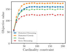
(a) Social graph

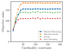
(b) Facebook ego network

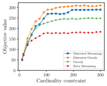
(c) EU Email

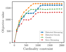
(d) Wikipedia vote

Figure 1: Directed vertex cover: we compare objective values by varying the cardinality constraint $k$.

6.2 Mode Finding of SLC Distributions: Experimental Evaluations

In this section, we compare the performance of Distorted-Streaming with the performance of distorted greedy, vanilla greedy and sieve streaming on the problem of mode finding for an SLR distribution. We consider a distribution $\nu(S)\propto\sqrt{\det\left(L_{S}\right)}\cdot\mathbf{1}\{|S|\leq d\}$, where $L$ is an $n\times n$ PSD matrix. Here, $L_{S}$ corresponds to the submatrix of $L$, where the rows and columns are indexed by elements of $S$ [53]. In the optimization procedure, our goal is to maximize $\rho(S)\triangleq\log(\nu(S))$. To generate the random matrix $L$, we first sample a diagonal matrix $D$ and a random PSD matrix $Q$, and then assign $L=QDQ^{-1}$. Each diagonal element of $D$ is from a log-normal distribution with a probability mass function $p(x)=\frac{1}{\sigma x\sqrt{2\pi}}\exp(-\frac{(\ln(x)-\mu)^{2}}{2\sigma^{2}})$, where $\mu$ and $\sigma$ are the mean and standard deviation of the normally distributed logarithm of the variable, respectively. This log-normal distribution allows us to have a PSD matrix where the eigenvalues have a heavy-tailed distribution. In these experiments, we set $n=1000,d=100,\mu=1.0$ and $\sigma=1.0$.

In Fig. 2, we observe that the outcome of Distorted-Streaming outperforms sieve streaming. This is mainly a result of the fact that Distorted-Streaming estimates the value of $\beta_{\text{{{OPT}}}}$ and uses the best possible value for $r$. Furthermore, we see that vanilla greedy performs better than distorted greedy, and for cardinality constraints larger than $k=20$, the performance of distorted greedy degrades. This observation could be explained by the fact that the linear cost for each element $u$ is comparable to the value of $g(u)$ (or marginal gain of $u$ to any set $S$). Therefore, distorted greedy does not pick any element in the first few iterations when $k$ is large enough, i.e., when $(1-\frac{1}{k})^{k-(i+1)}$ is small. It is worth mentioning that while the performance of the greedy algorithm is the best for this specific application, only Distorted-Streaming and distorted greedy have a theoretical guarantee.

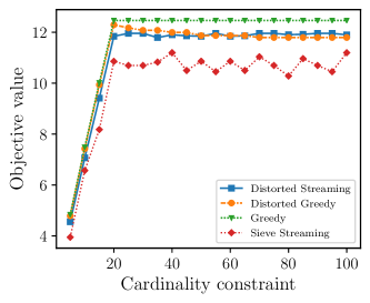
Figure 2: We want to find the mode of a distribution $\nu(S)\propto\sqrt{\det\left(L_{S}\right)}\cdot\mathbf{1}\{|S|\leq d\}$ for a PSD matrix $L$. For the objective value, we report $\log(\nu(S))$.

6.3 Distributed Setting

In this section, we compare Distorted-Distributed-Greedy with the distributed greedy algorithm of Barbosa et al. [5]. We evaluate the performance of these algorithms over several large graphs [38] in the setting of Section 6.1 under a cardinality constraint $k=\numprint{1000}$, where we set $q=50$. For both algorithms, we set the number of computational rounds to 10. The first graph is the Amazon product co-purchasing network with $n=\numprint{334863}$ vertices; the second one is the DBLP collaboration network with $n=\numprint{317080}$ vertices; the third graph is Youtube with $n=\numprint{1134890}$ vertices; and the last graph we consider is the Pokec social network, the most popular online social network in Slovakia, with $n=\numprint{1632803}$ vertices. For each graph, we set the number of machines to $m=\lceil\nicefrac{{n}}{{4000}}\rceil$. From Fig. 3, we can see that the objective values of Distorted-Distributed-Greedy exceed the results of distributed greedy for all four graphs.

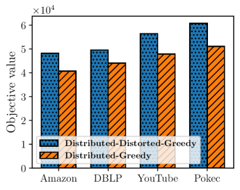
Figure 3: We compare the Distorted-Distributed-Greedy with the distributed greedy algorithm under a cardinality constraint with $k=\numprint{1000}$. The number of computational rounds is set to 10.

6.4 Regularized Data Summarization

In this section, through an extensive set of experiments, we answer the following two questions:

• How does Distorted-Streaming perform with respect to sieve-streaming and distorted greedy on real-world data summarization tasks?

• Is our proposed modeling approach (maximizing diversity while considering costs of items as a regularization term in a single function) favorable to methods which try to maximize a submodular function subject to a knapsack constraint?

We consider three state-of-the-art algorithms for solving the problem of submodular maximization with a cardinality and a knapsack constraint: FANTOM [45], Fast [2] and Vanilla Greedy Dynamic Program [48]. For the sake of fairness of our experiments, we used these three algorithms to maximize the submodular function $g$ under 50 different knapsack capacities $c$ in the interval $0.1\leq c\leq 100$ and reported the solution maximizing $g(S)-\ell(S)$. We note that, for the computational complexities of these algorithms, we report the number of oracle calls used by a single one out of their 50 runs (one for each different knapsack capacity), which gives these offline algorithms a considerable edge in our comparisons.

6.4.1 Online Video Summarization

In this task, we consider the online video summarization application, where a stream of video frames comes, and one needs to provide a set of $k$ representative frames as the summary of the whole video. In this application, the objective is to select a subset of frames in order to maximize a utility function $g(S)$ (which represents the diversity), while minimizing the total entropy of the selection. We use a non-negative modular function $\ell(S)$ to represent the entropy of the set $S$, which could be interpreted as a proxy of the storage size of $S$.

We used the pre-trained ResNet-18 model [29] to extract features from frames of each video. Then, given a set of frames, we defined a matrix $M$ such that $M_{ij}=e^{-\textrm{dist}(x_{i},x_{j})}$, where $\text{dist}(x_{i},x_{j})$ denotes the distance between the feature vectors of the $i$-th and $j$-th frames, respectively. One can think of $M$ as a similarity matrix among different frames of a video. The utility of a set $S\subseteq V$ is defined as a non-negative and monotone submodular objective $g(S)=\log\det(\mathbf{I}+\alpha M_{S})$, where $\mathbf{I}$ is the identity matrix, $\alpha$ is a positive scalar and $M_{S}$ is the principal sub-matrix of the similarity matrix $M$ indexed by $S$. Informally, this function is meant to measure the diversity of the vectors in $S$. To sum-up, we want to maximize the following function under a cardinality constraint $k$: $f(S)\triangleq g(S)-\ell(S)=\log\det(\mathbf{I}+\alpha M_{S})-\sum_{u\in S}\mathrm{H}_{u},$ where $\mathrm{H}_{u}$ represents the entropy of frame $u$.

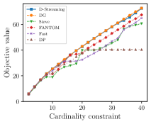
(a) Video number 13

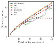
(b) Video number 15

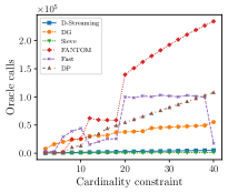
(c) Video number 13

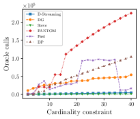
(d) Video number 15

(e) The summaries produced by Distorted-Streaming for video number 14.

Figure 4: Movie frame summarization: For each frame $u$ the linear cost $\ell_{u}$ is the entropy of that frame. (a) and (b) compare the objective values. (c) and (d) compare the computational complexities based on the number of oracle calls. In experiment (e), the input function is $f(S)\triangleq g(S)-\lambda\cdot\ell(S)$ for $\lambda\in\{0,0.5,1.0\}$, where we set the cardinality constraint to $k=6$.

In the first experiment, we summarized the frames of videos 13 and 15 from the VSUMM dataset [12], and compare the above mentioned algorithms based on their objective values and number of oracle values for varying cardinality constraint $k$. From Figs. 4a and 4b we conclude that (i) the quality of the solutions returned by Distorted-Streaming is as good as the quality of the results of distorted greedy, (ii) distorted greedy clearly outperforms sieve-streaming, and (iii) the objective values of Distorted-Streaming and distorted greedy are both larger than the corresponding values produced by Greedy Dynamic Program, Fast and FANTOM. This confirms that directly maximizing the function $f$ provides higher utilities versus maximizing the function $g$ and setting a knapsack constraint over the modular function $\ell$. In Figs. 4c and 4d, we observe that the computational complexity of Distorted-Streaming and sieve streaming is several orders of magnitudes better than the computation complexity of the other algorithms, which is consistent with their need to make only a single pass over the data.

Next, we study the effect of the linear cost function (in the other words, the importance we give to the entropy of frames) on the set of selected frames. For this reason, we run Distorted-Streaming on the frames from video number 14. The objective function is $f(S)\triangleq g(S)-\lambda\cdot\ell(S)$ for $\lambda\in\{0,0.5,1.0\}$. In this experiment, we set the cardinality constraint to $k=6$. In Fig. 4e, we observe that by increasing $\lambda$ the entropy of the selected frames decreases. This is evident from the fact that the color diversity of pixels in each frame reduces for larger values of $\lambda$. Consequently, the representativeness of the selected subset decreases. Indeed, while it is easy to understand the whole story of this animation from the output produced for $\lambda=0$, some parts of the story are definitely missing if we set $\lambda$ to $1.0$.

6.4.2 Yelp Location Summarization

In this summarization task, we want to summarize a dataset of business locations. For this reason, we consider a subset of Yelp’s businesses, reviews and user data [61], referred to as the Yelp Academic dataset [60]. This dataset contains information about local businesses across 11 metropolitan areas. The features for each location are extracted from the description of that location and related user reviews. The extracted features cover information regarding several attributes, including parking options, WiFi access, having vegan menus, delivery options, possibility of outdoor seating, being good for groups.

The goal is to choose a subset of businesses locations, out of a ground set $\cN=\{1,\dots,n\}$, which provides a good summary of all the existing locations. We calculated the similarity matrix $M\in\bR^{n\times n}$ between locations using the same method described in Section 6.4.1. For a selected set $S$, we assume each location $i\in\cN$ is represented by the location from the set $S$ with the highest similarity to $i$. This makes it natural to define the total utility provided by set $S$ using the set function

$$f(S)\triangleq g(S)-\ell(S)=\frac{1}{n}\sum_{i=1}^{n}\max_{j\in S}M_{i,j}-\sum_{u\in S}\ell_{u}\enspace.$$ (6)

Note that $g(S)$ is monotone and submodular [34, 22]. For the linear function $\ell$ we consider two scenarios: (i) in the first one, the cost assigned to each location is defined as its distance to the downtown in the city of that location. ii) in the second scenario, the linear cost of each location $u$ is the distance between $u$ and the closest international airport in that area. The intuitive explanation of the first linear function is that while we look for the most diverse subset of locations as our summary, we want those locations to be also close enough to the down-town in order to make commute and access to other facilities easier. For the second linear function, we want the selected locations to be in the vicinity of airports.

From Eq. 6 it is evident that computing the objective function requires access to the entire dataset $\cN$, which in the streaming setting is not possible. Fortunately, however, this function is additively decomposable [44] over the ground set $\cN$. Therefore, it is possible to estimate Eq. 6 arbitrarily close to its exact value as long as we can sample uniformly at random from the data stream [3, Proposition 6.1]. In this section, to sample randomly from the data stream and to have an accurate estimate of the function, we use the reservoir sampling technique explained in [3, Algortithm 4].

In Fig. 5, we compare algorithms for varying values of $k$ while we consider the two different linear functions $\ell$. We observe that distorted greedy returns the solutions with the highest utilities. The performance of Distorted-Streaming is comparable with that of the offline algorithms, and it clearly surpasses sieve-streaming. In addition, our experiments demonstrate that Distorted-Streaming (and similarly sieve-streaming) requires orders of magnitude fewer oracle evaluations.

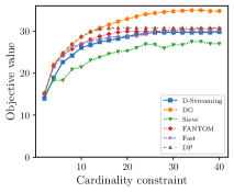
(a) $\ell=$ distance to down-town

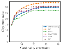
(b) $\ell=$ distance to airport

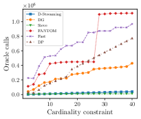
(c) $\ell=$ distance to down-town

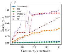
(d) $\ell=$ distance to airport

Figure 5: Yelp location summarization: data points are locations from six different cities. For the linear costs we consider two different cases: 1) distances to the downtown in each city, 2) distances to the airport in each city.

6.4.3 Movie Recommendation

In this application, the goal is to recommend a set of movies to a user, where we know that the user is mainly interested in movies released around 1990. As a matter of fact, we are aware that her all-time favorite movie is Goodfellas (1990). To design our recommender system, we use ratings from MovieLens users [27], and apply the method of Lindgren et al. [40] to generate a set of features for each movie.

For a ground set of movies $\cN$, assume $v_{i}$ represents the feature vector of the $i$-th movie. Following the same approach we used in Section 6.4.1, we define a similarity matrix $M$ such that $M_{ij}=e^{-\text{dist}(v_{i},v_{j})}$, where $\text{dist}(v_{i},v_{j})$ is the euclidean distance between vectors $v_{i},v_{j}\in\cN$. The objective of each algorithm is to select a subset of movies that maximizes $f(S)\triangleq g(S)-\ell(S)=\log\det(\mathbf{I}+\alpha M_{S})-\sum_{v\in S}\ell_{v}$ subject to a cardinality constraint $k$. In this application for $\ell(S)=\sum_{v\in S}\ell_{v}$ we consider two different scenarios: (i) $\ell_{v}=\lvert 1990-\textrm{year}_{v}\rvert$, where $\textrm{year}_{v}$ denote the release year of movie $v$, and (2) $\ell_{v}=10-\textrm{rating}_{v}$, where $\textrm{rating}_{v}$ denotes the IMDb rating of $v$ ($10$ is the maximum possible rating).

From our experimental evaluation in Fig. 6, we observe that both modeling approaches (directly maximizing the function $f$ and maximizing the function $g$ subject to a knapsack constraint for $\ell$) return solutions with similar objective values. Besides, we note that the computational complexity of Distorted-Streaming is better than the complexity of the expensive offline algorithms (as it makes only a single pass over the data), but this difference is not very significant for some offline algorithms. Nevertheless, Distorted-Streaming always provides better utility than sieve streaming.

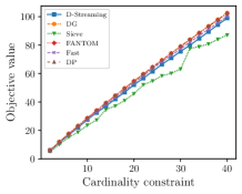
(a) $\ell_{v}=\lvert 1990-\textrm{year}_{v}\rvert$

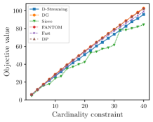
(b) $\ell_{v}=\lvert 10-\textrm{rating}_{v}\rvert$

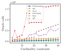
(c) $\ell_{v}=\lvert 1990-\textrm{year}_{v}\rvert$

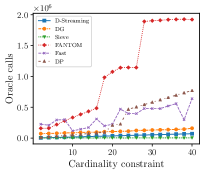
(d) $\ell_{v}=\lvert 10-\textrm{rating}_{v}\rvert$

Figure 6: Movie recommendation: we compare algorithms for varying cardinality constraint $k$. We use two different linear functions: $\lvert 1990-\textrm{year}_{v}\rvert$ and $10-\textrm{rating}_{v}$, where the goal of first one is to recommend movies with a release year closer to 1990 and the goal of the second linear function is to promote movies with higher ratings.

6.4.4 Twitter Text Summarization

There are several news-reporting Twitter accounts with millions of followers. In this section, our goal is to produce real-time summaries for Twitter feeds of a subset of these accounts. In the Twitter stream summarization task, one might be interested in a representative and diverse summary of events that happen around a certain date. For this application, we consider the Twitter dataset provided in [32], where the keywords from each tweet are extracted and weighted proportionally to the number of retweets the post received. Let $\cW$ denote the set of all existing keywords. The function $f$ we want to maximize is defined over a ground set $\cN$ of tweets [32]. Assume each tweet $e\in\cN$ consists of a positive value $\textrm{val}_{e}$ representing the number of retweets it has received (as a measure of the popularity and importance of that tweet) and a set of $l_{e}$ keywords $\cW_{e}=\{w_{e,1},\cdots,w_{e,l_{e}}\}$ from $\cW$. The score of a word $w\in\cW_{e}$ with respect to a given tweet $e$ is calculated by $\text{score}(w,e)=\text{val}_{e}$. If $w\notin\cW_{e}$, we assume $\text{score}(w,e)=0$. Formally, the function $f$ is defined as follows:

$$f(S)\triangleq g(S)-\ell(S)=\sum_{w\in\cW}\sqrt{\sum_{e\in S}\text{score}(w,e)}-\sum_{e\in S}\ell_{e}\enspace,$$

where for the linear function $\ell$ two options are considered: (i) $\ell_{e}=|01/01/2019-\textrm{T}(e)|$ is the absolute difference (in number months) between time of tweet $e$ and the first of January 2019, (ii) $\ell_{e}=|\cW_{e}|$ is the length of each tweet, which enables us to provide shorter summaries. Note that the monotone and submodular function $g$ is designed to cover the important events of the day without redundancy (by encouraging diversity in a selected set of tweets) [32].

The main observation from Fig. 7 is that Distorted-Streaming clearly outperforms the sieve-streaming algorithm and the Greedy Dynamic Program algorithm in terms of objective value, where the gap between their performances grows for larger values of $k$. The utility of other offline algorithms is slightly better than that of our proposed streaming algorithm. We also see that while distorted greedy is by far the fastest offline algorithm, the computational complexities of both streaming algorithms are negligible with respect to the other offline algorithms.

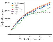
(a) $\ell_{e}=|01/01/2019-\textrm{T}(e)|$

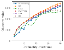
(b) $\ell_{e}=|\cW_{e}|$

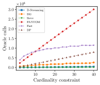
(c) $\ell_{e}=|01/01/2019-\textrm{T}(e)|$

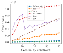
(d) $\ell_{e}=|\cW_{e}|$

Figure 7: Twitter text summarization: We compare algorithms for varying values of the cardinality constraint $k$. In figures (a) and (c) the linear cost is the difference between the time of the tweet and the first of January 2019. In figures (b) and (d) the linear cost is the number of keywords in each tweet.

7 Conclusion

In this paper, we proposed scalable methods for maximizing a regularized submodular function expressed as the difference between a non-negative monotone submodular function $g$ and a modular function $\ell$. We developed the first one-pass streaming algorithm for maximizing a regularized submodular function subject to a $k$-cardinality constraint with a theoretical performance guarantee, and also presented the first distributed algorithm that returns a solution $S$ with the guarantee that $\bE[f(S)]\geq(1-\varepsilon)\left[(1-e^{-1})\cdot g(OPT)-\ell(OPT)\right]$ in $O(1/\varepsilon)$ rounds of MapReduce computation. Moreover, even for the unregularized case, our distributed algorithm improves the memory and communication complexity of the existing work by a factor of $O(1/\varepsilon)$ while providing a simpler distributed algorithm and a unifying analysis. We also empirically studied the performance of our scalable methods on a set of real-life applications, including vertex cover of social networks, finding the mode of strongly log-concave distributions, data summarization, and product recommendation.

Appendix A Guessing $\tau$ in Algorithm 1

In this section we explain how one can guess the value $\tau$ in Algorithm 1, which is a value obeying $k\tau\leq h(r)\cdot g(T)-r\cdot\ell(T)\leq(1+\varepsilon)k\tau$, at the cost of increasing the space complexity of the algorithm by a factor of $O(\varepsilon^{-1}(\log k+\log r^{-1}))$. Like in Section 3.2, we assume that $h(r)\cdot g(T)-r\cdot\ell(T)$—and thus, also $\tau$—is positive.

Observe that

$$\max_{u\in\cN}[h(r)\cdot g(\{u\})-r\cdot\ell(\{u\})]\leq{} h(r)\cdot g(T)-r\cdot\ell(T)\leq\sum_{u\in T}[h(r)\cdot g(\{u\})-r\cdot\ell(\{u\})]$$

$$\leq{} k\cdot\max_{u\in\cN}[h(r)\cdot g(\{u\})-r\cdot\ell(\{u\})]\enspace,$$

where the first inequality holds since $\{u\}$ is a candidate to be $T$ for every $u\in\cN$, and the second inequality follows from the submodularity of $g$. Thus, if we knew the value of $\max_{u\in\cN}[h(r)\cdot g(\{u\})-r\cdot\ell(\{u\})]$ from the very beginning, we could simply run in parallel an independent copy of Algorithm 1 for every value of $\tau$ that has the form $(1+\varepsilon)^{i}$ for some integer $i$ and falls within the range

$$\left[k^{-1}\cdot\max_{u\in\cN}[h(r)\cdot g(\{u\})-r\cdot\ell(\{u\})],(1+\varepsilon)\cdot\max_{u\in\cN}[h(r)\cdot g(\{u\})-r\cdot\ell(\{u\})]\right]\enspace.$$

Clearly, at least one of the values we would have tried obeys $k\tau\leq h(r)\cdot g(T)-r\cdot\ell(T)\leq(1+\varepsilon)k\tau$, and the number of values we would have needed to try is upper bounded by

$$1+\log_{1+\varepsilon}\left(\frac{(1+\varepsilon)\cdot\max_{u\in\cN}[h(r)\cdot g(\{u\})-r\cdot\ell(\{u\})}{k^{-1}\cdot\max_{u\in\cN}[h(r)\cdot g(\{u\})-r\cdot\ell(\{u\})]}\right)=2+\log_{1+\varepsilon}k=O(\varepsilon^{-1}\log k)\enspace.$$

Unfortunately, the value of $\max_{u\in\cN}[h(r)\cdot g(\{u\})-r\cdot\ell(\{u\})]$ is not known to us in advance. To compensate for this, we make the following two observations. The first observation is that $k^{-1}\cdot\max_{u\in\cN^{\prime}}[h(r)\cdot g(\{u\})-r\cdot\ell(\{u\})]$, where $\cN^{\prime}$ is the set of elements viewed so far, is a lower bound on the value of $k^{-1}\cdot\max_{u\in\cN}[h(r)\cdot g(\{u\})-r\cdot\ell(\{u\})]$. Following is the second observation, which shows that copies of Algorithm 1 with $\tau$ values that are much larger than this lower bound cannot accept any element of $\cN^{\prime}$, and thus, need not be maintained explicitly.

Observation 17.

If $\tau>(\alpha(r)/r)\cdot\max_{u\in\cN^{\prime}}[h(r)\cdot g(\{u\})-r\cdot\ell(\{u\})]$, then Algorithm 1 accepts no element of $\cN^{\prime}$.

Proof.

Algorithm 1 accepts an element $u\in\cN^{\prime}$ if $g(u\mid S)-\alpha(r)\cdot\ell(\{u\})\geq\tau$. However, the condition of the observation implies

$$g(u\mid S)-\alpha(r)\cdot\ell(\{u\})\leq{} g(\{u\})-\alpha(r)\cdot\ell(\{u\})=\frac{\alpha(r)}{r}\cdot[h(r)\cdot g(\{u\})-r\cdot\ell(\{u\})]$$

$$\leq{} \frac{\alpha(r)}{r}\cdot\max_{u\in\cN^{\prime}}[h(r)\cdot g(\{u\})-r\cdot\ell(\{u\})]<\tau\enspace,$$

where the first inequality follows from the submodularity of $g$, and the equality follows from the following calculation.

$$\alpha(r)\cdot h(r)=\frac{2r+1+\sqrt{4r^{2}+1}}{2}\cdot\frac{2r+1-\sqrt{4r^{2}+1}}{2}=\frac{(2r+1)^{2}-(4r^{2}+1)}{4}=\frac{4r}{4}=r\enspace.\qed$$

The above observations imply that it suffices to explicitly maintain a copy of Algorithm 1 for values of $\tau$ that are equal to $(1+\varepsilon)^{i}$ for some integer $i$ and fall within the range

$$\left[k^{-1}\cdot\max_{u\in\cN^{\prime}}[h(r)\cdot g(\{u\})-r\cdot\ell(\{u\})],\frac{\alpha(r)}{r}\cdot\max_{u\in\cN^{\prime}}[h(r)\cdot g(\{u\})-r\cdot\ell(\{u\})]\right]\enspace.$$ (7)

In particular, we know that when the value of $\max_{u\in\cN^{\prime}}[h(r)\cdot g(\{u\})-r\cdot\ell(\{u\})]$ increases (due to the arrival of additional elements), we can start a new copy of Algorithm 1 for the values of $\tau$ that have the form $(1+\varepsilon)^{i}$ for some integer $i$ and now enter the range. By Observation 17, these instances will behave in exactly the same way as if they had been created at the very beginning of the stream. A formal description of the algorithm we obtain using this method is given as Algorithm 4. We note that the space complexity of this algorithm is larger than the space complexity of Algorithm 1 only by an $O(\varepsilon^{-1}(\log k+\log r^{-1}))$ factor because the number of values of the form $(1+\varepsilon)^{i}$ that can fall within the range (7) is at most

$$\mspace{-100.0mu}1+\log_{1+\varepsilon}\left(\frac{\frac{\alpha(r)}{r}\cdot\max_{u\in\cN^{\prime}}[h(r)\cdot g(\{u\})-r\cdot\ell(\{u\})]}{k^{-1}\cdot\max_{u\in\cN^{\prime}}[h(r)\cdot g(\{u\})-r\cdot\ell(\{u\})]}\right)=1+\log_{1+\varepsilon}\left(\frac{k\cdot\alpha(r)}{r}\right)$$

$$={} 1+\log_{1+\varepsilon}\left(\frac{k\cdot(2r+1+\sqrt{4r^{2}+1})}{2r}\right)\leq 1+\log_{1+\varepsilon}(k+k/r)$$

$$\leq{} 1+\log_{1+\varepsilon}k+\log_{1+\varepsilon}(k/r)=O(\varepsilon^{-1}(\log k+\log r^{-1}))\enspace.$$

Let $M\leftarrow-\infty$ and $I\leftarrow\varnothing$.

  // $M$ represents $\max_{u\in\cN^{\prime}}[h(r)\cdot g(\{u\})-r\cdot\ell(\{u\})]$ and $I$ is the list of copies of Algorithm 1 currently maintained.

1 while there are more elements in the stream do

2       Let $u$ be the next element of the stream.

3       Update $M\leftarrow\max\{M,h(r)\cdot g(\{u\})-r\cdot\ell(\{u\})\}$.

4       Let $J=\{i\in\bZ\mid k^{-1}M\leq(1+\varepsilon)^{i}\leq r^{-1}M\cdot\alpha(r)\}$.

5       Delete every copy of Algorithm 1 in $I$ corresponding to a value $\tau=(1+\varepsilon)^{i}$ for an integer $i$ that now falls outside the set $J$.

6       Add to $I$ a new copy of Algorithm 1 with $\tau=(1+\varepsilon)^{i}$ for every integer $i\in J$, unless such a copy already exists there.

7       Pass the element $u$ to all the copies of Algorithm 1 in $I$.

return the set $S$ maximizing $g(S)-\ell(S)$ among all the output sets of all the copies of Algorithm 1 in $I$.

Algorithm 4 Distorted-Streaming: Guessing $\tau$

References

- Alaluf and Feldman [2019] Naor Alaluf and Moran Feldman. Making a sieve random: Improved semi-streaming algorithm for submodular maximization under a cardinality constraint. CoRR, abs/1906.11237, 2019. URL http://arxiv.org/abs/1906.11237.
- Badanidiyuru and Vondrák [2014] Ashwinkumar Badanidiyuru and Jan Vondrák. Fast algorithms for maximizing submodular functions. In ACM-SIAM symposium on Discrete algorithms (SODA), pages 1497–1514, 2014.
- Badanidiyuru et al. [2014] Ashwinkumar Badanidiyuru, Baharan Mirzasoleiman, Amin Karbasi, and Andreas Krause. Streaming Submodular Maximization:Massive Data Summarization on the Fly. In International Conference on Knowledge Discovery and Data Mining, KDD, pages 671–680, 2014.
- Barbosa et al. [2015] Rafael da Ponte Barbosa, Alina Ene, Huy Nguyen, and Justin Ward. The power of randomization: Distributed submodular maximization on massive datasets. In International Conference on Machine Learning, pages 1236–1244, 2015.
- Barbosa et al. [2016] Rafael da Ponte Barbosa, Alina Ene, Huy L. Nguyen, and Justin Ward. A New Framework for Distributed Submodular Maximization. In Symposium on Foundations of Computer Science, (FOCS), pages 645–654, 2016.
- Borcea et al. [2009] Julius Borcea, Petter Brändén, and Thomas Liggett. Negative dependence and the geometry of polynomials. Journal of the American Mathematical Society, 22(2):521–567, 2009.
- Buchbinder and Feldman [2018] Niv Buchbinder and Moran Feldman. Submodular Functions Maximization Problems. In Handbook of Approximation Algorithms and Metaheuristics, pages 771–806. Chapman and Hall/CRC, 2018.
- Buchbinder et al. [2015] Niv Buchbinder, Moran Feldman, and Roy Schwartz. Online submodular maximization with preemption. In ACM-SIAM Symposium on Discrete Algorithms, SODA, pages 1202–1216, 2015.
- Chakrabarti and Kale [2015] Amit Chakrabarti and Sagar Kale. Submodular maximization meets streaming: matchings, matroids, and more. Math. Program., 154(1-2):225–247, 2015.
- Chekuri et al. [2015] Chandra Chekuri, Shalmoli Gupta, and Kent Quanrud. Streaming algorithms for submodular function maximization. In International Colloquium on Automata, Languages, and Programming, pages 318–330. Springer, 2015.
- Das and Kempe [2011] Abhimanyu Das and David Kempe. Submodular meets spectral: greedy algorithms for subset selection, sparse approximation and dictionary selection. In International Conference on Machine Learning, pages 1057–1064, 2011.
- De Avila et al. [2011] Sandra Eliza Fontes De Avila, Ana Paula Brandão Lopes, Antonio da Luz Jr, and Arnaldo de Albuquerque Araújo. Vsumm: A mechanism designed to produce static video summaries and a novel evaluation method. Pattern Recognition Letters, 32(1):56–68, 2011.
- Djolonga and Krause [2014] Josip Djolonga and Andreas Krause. From map to marginals: Variational inference in bayesian submodular models. In Advances in Neural Information Processing Systems, pages 244–252, 2014.
- Elenberg et al. [2017] Ethan R. Elenberg, Alexandros G. Dimakis, Moran Feldman, and Amin Karbasi. Streaming Weak Submodularity: Interpreting Neural Networks on the Fly. In Advances in Neural Information Processing Systems, pages 4047–4057, 2017.
- Elenberg et al. [2018] Ethan R Elenberg, Rajiv Khanna, Alexandros G Dimakis, Sahand Negahban, et al. Restricted strong convexity implies weak submodularity. The Annals of Statistics, 46(6B):3539–3568, 2018.
- Ene et al. [2019] Alina Ene, Huy L. Nguyen, and Andrew Suh. An optimal streaming algorithm for non-monotone submodular maximization. CoRR, abs/1911.12959, 2019. URL http://arxiv.org/abs/1911.12959.
- Feige et al. [2011] Uriel Feige, Vahab S. Mirrokni, and Jan Vondrák. Maximizing non-monotone submodular functions. SIAM J. Comput., 40(4):1133–1153, 2011.
- Feldman [2019] Moran Feldman. Guess free maximization of submodular and linear sums. In Algorithms and Data Structures (WADS), pages 380–394, 2019.
- Feldman et al. [2011] Moran Feldman, Joseph Naor, Roy Schwartz, and Justin Ward. Improved approximations for k-exchange systems - (extended abstract). In ESA, pages 784–798, 2011.
- Feldman et al. [2017] Moran Feldman, Christopher Harshaw, and Amin Karbasi. Greed is good: Near-optimal submodular maximization via greedy optimization. In COLT, pages 758–784, 2017.
- Feldman et al. [2018] Moran Feldman, Amin Karbasi, and Ehsan Kazemi. Do Less, Get More: Streaming Submodular Maximization with Subsampling. In Advances in Neural Information Processing Systems, pages 730–740, 2018.
- Frieze [1974] Alan M Frieze. A cost function property for plant location problems. Mathematical Programming, 7(1):245–248, 1974.
- Gotovos [2019] Alkis Gotovos. Strong log-concavity does not imply log-submodularity. arXiv preprint arXiv:1910.11544, 2019.
- Gotovos et al. [2015] Alkis Gotovos, Hamed Hassani, and Andreas Krause. Sampling from probabilistic submodular models. In Advances in Neural Information Processing Systems, pages 1945–1953, 2015.
- Gurvits [2009] Leonid Gurvits. A polynomial-time algorithm to approximate the mixed volume within a simply exponential factor. Discrete & Computational Geometry, 41(4):533–555, 2009.
- Gygli et al. [2015] Michael Gygli, Helmut Grabner, and Luc Van Gool. Video summarization by learning submodular mixtures of objectives. In IEEE conference on computer vision and pattern recognition, pages 3090–3098, 2015.
- Harper and Konstan [2015] F Maxwell Harper and Joseph A Konstan. The movielens datasets: History and context. Acm transactions on interactive intelligent systems (tiis), 5(4):1–19, 2015.
- Harshaw et al. [2019] Chris Harshaw, Moran Feldman, Justin Ward, and Amin Karbasi. Submodular Maximization beyond Non-negativity: Guarantees, Fast Algorithms, and Applications. In International Conference on Machine Learning, pages 2634–2643, 2019.
- He et al. [2016] Kaiming He, Xiangyu Zhang, Shaoqing Ren, and Jian Sun. Deep Residual Learning for Image Recognition. In computer vision and pattern recognition (CVPR), pages 770–778, 2016.
- Iyer and Bilmes [2015] Rishabh Iyer and Jeffrey Bilmes. Submodular point processes with applications to machine learning. In Artificial Intelligence and Statistics, pages 388–397, 2015.
- Kazemi et al. [2018] Ehsan Kazemi, Morteza Zadimoghaddam, and Amin Karbasi. Scalable Deletion-Robust Submodular Maximization: Data Summarization with Privacy and Fairness Constraints. In International Conference on Machine Learning (ICML), pages 2549–2558, 2018.
- Kazemi et al. [2019] Ehsan Kazemi, Marko Mitrovic, Morteza Zadimoghaddam, Silvio Lattanzi, and Amin Karbasi. Submodular Streaming in All Its Glory: Tight Approximation, Minimum Memory and Low Adaptive Complexity. In International Conference on Machine Learning (ICML), pages 3311–3320, 2019.
- Kirchhoff and Bilmes [2014] Katrin Kirchhoff and Jeff Bilmes. Submodularity for data selection in statistical machine translation. In Proceedings of EMNLP, 2014.
- Krause and Golovin [2012] Andreas Krause and Daniel Golovin. Submodular Function Maximization. In Tractability: Practical Approaches to Hard Problems. Cambridge University Press, 2012.
- Kulesza and Taskar [2012] Alex Kulesza and Ben Taskar. Determinantal Point Processes for Machine Learning. Foundations and Trends® in Machine Learning, 5(2–3):123–286, 2012.
- Kumar et al. [2015] Ravi Kumar, Benjamin Moseley, Sergei Vassilvitskii, and Andrea Vattani. Fast Greedy Algorithms in MapReduce and Streaming. TOPC, 2(3):14:1–14:22, 2015.
- Lee et al. [2010] Jon Lee, Vahab S. Mirrokni, Viswanath Nagarajan, and Maxim Sviridenko. Maximizing nonmonotone submodular functions under matroid or knapsack constraints. SIAM J. Discrete Math., 23(4):2053–2078, 2010.
- Leskovec and Krevl [2014] Jure Leskovec and Andrej Krevl. SNAP Datasets: Stanford Large Network Dataset Collection. http://snap.stanford.edu/data, June 2014.
- Lin and Bilmes [2011] Hui Lin and Jeff A. Bilmes. A Class of Submodular Functions for Document Summarization. In HLT, pages 510–520, 2011.
- Lindgren et al. [2015] Erik M Lindgren, Shanshan Wu, and Alexandros G Dimakis. Sparse and greedy: Sparsifying submodular facility location problems. In NeurIPS Workshop on Optimization for Machine Learning, 2015.
- Liu and Vondrák [2018] Paul Liu and Jan Vondrák. Submodular Optimization in the MapReduce Model. CoRR, abs/1810.01489, 2018.
- Lovász [1983] László Lovász. Submodular functions and convexity. In Mathematical Programming The State of the Art, pages 235–257. Springer, 1983.
- Mirrokni and Zadimoghaddam [2015] Vahab Mirrokni and Morteza Zadimoghaddam. Randomized composable core-sets for distributed submodular maximization. In Ssymposium on Theory of Computing (STOC), pages 153–162. ACM, 2015.
- Mirzasoleiman et al. [2013] Baharan Mirzasoleiman, Amin Karbasi, Rik Sarkar, and Andreas Krause. Distributed submodular maximization: Identifying representative elements in massive data. In Advances in Neural Information Processing Systems, pages 2049–2057, 2013.
- Mirzasoleiman et al. [2016a] Baharan Mirzasoleiman, Ashwinkumar Badanidiyuru, and Amin Karbasi. Fast Constrained Submodular Maximization: Personalized Data Summarization. In ICML, pages 1358–1367, 2016a.
- Mirzasoleiman et al. [2016b] Baharan Mirzasoleiman, Amin Karbasi, Rik Sarkar, and Andreas Krause. Distributed Submodular Maximization. Journal of Machine Learning Research (JMLR), 17:1–44, 2016b.
- Mitrovic et al. [2018] Marko Mitrovic, Ehsan Kazemi, Morteza Zadimoghaddam, and Amin Karbasi. Data Summarization at Scale: A Two-Stage Submodular Approach. In International Conference on Machine Learning (ICML), pages 3593–3602, 2018.
- Mizrachi et al. [2019] Eyal Mizrachi, Roy Schwartz, Joachim Spoerhase, and Sumedha Uniyal. A Tight Approximation for Submodular Maximization with Mixed Packing and Covering Constraints. In International Colloquium on Automata, Languages, and Programming, (ICALP), pages 85:1–85:15, 2019.
- Nemhauser and Wolsey [1978] G. L. Nemhauser and L. A. Wolsey. Best Algorithms for Approximating the Maximum of a Submodular Set Function. Mathematics of Operations Research, 3(3):177–188, 1978.
- Nemhauser et al. [1978] George L Nemhauser, Laurence A Wolsey, and Marshall L Fisher. An analysis of approximations for maximizing submodular set functions—i. Mathematical Programming, 14(1):265–294, 1978.
- Norouzi-Fard et al. [2018] Ashkan Norouzi-Fard, Jakub Tarnawski, Slobodan Mitrovic, Amir Zandieh, Aidasadat Mousavifar, and Ola Svensson. Beyond 1/2-Approximation for Submodular Maximization on Massive Data Streams. In International Conference on Machine Learning (ICML), pages 3826–3835, 2018.
- Rebeschini and Karbasi [2015] Patrick Rebeschini and Amin Karbasi. Fast mixing for discrete point processes. In Conference on Learning Theory, pages 1480–1500, 2015.
- Robinson et al. [2019] Joshua Robinson, Suvrit Sra, and Stefanie Jegelka. Flexible Modeling of Diversity with Strongly Log-Concave Distributions. In Advances in Neural Information Processing Systems, pages 15199–15209, 2019.
- Salehi et al. [2017] Mehraveh Salehi, Amin Karbasi, Dustin Scheinost, and R Todd Constable. A submodular approach to create individualized parcellations of the human brain. In International Conference on Medical Image Computing and Computer-Assisted Intervention, pages 478–485. Springer, 2017.
- Sviridenko et al. [2017] Maxim Sviridenko, Jan Vondrák, and Justin Ward. Optimal approximation for submodular and supermodular optimization with bounded curvature. Math. Oper. Res., 42(4):1197–1218, 2017.
- Tschiatschek et al. [2014a] Sebastian Tschiatschek, Rishabh K. Iyer, Haochen Wei, and Jeff A. Bilmes. Learning mixtures of submodular functions for image collection summarization. In NIPS, pages 1413–1421, 2014a.
- Tschiatschek et al. [2014b] Sebastian Tschiatschek, Rishabh K Iyer, Haochen Wei, and Jeff A Bilmes. Learning Mixtures of Submodular Functions for Image Collection Summarization. In Advances in neural information processing systems, pages 1413–1421, 2014b.
- Wei et al. [2015] Kai Wei, Rishabh Iyer, and Jeff Bilmes. Submodularity in data subset selection and active learning. In International Conference on Machine Learning, pages 1954–1963, 2015.
- Wei et al. [2016] Kai Wei, Maxwell W Libbrecht, Jeffrey A Bilmes, and William Stafford Noble. Choosing panels of genomics assays using submodular optimization. Genome biology, 17(1):229, 2016.
- Yelp [a] Yelp. Yelp Academic Dataset. https://www.kaggle.com/yelp-dataset/yelp-dataset, 2019a.
- Yelp [b] Yelp. Yelp Dataset. https://www.yelp.com/dataset, 2019b.