Variational Principle of Action and Group Theory for Bifurcation of Figure-eight solutions

Abstract

Figure-eight solutions are solutions to planar equal mass three-body problem under homogeneous or inhomogeneous potentials. They are known to be invariant under the transformation group $D_{6}$: the dihedral group of regular hexagons. Numerical investigation shows that each figure-eight solution has some bifurcation points. Six bifurcation patterns are known with respect to the symmetry of the bifurcated solution.

In this paper we will show the followings. The variational principle of action and group theory show that the bifurcations of every figure-eight solution are determined by the irreducible representations of $D_{6}$. Each irreducible representation has one to one correspondence to each bifurcation. This explains numerically observed six bifurcation patterns. In general, in Lagrangian mechanics, bifurcations of a periodic solution are determined by irreducible representations of the transformation group that leave this solution invariant.

Keywords: variational principle, action, group theory, bifurcation, figure-eight

1 Introduction

The aim of this paper is to give a theoretical explanation for bifurcations of figure-eight solutions using the variational principle of action and group theory.

The plan of this paper is the following: Section 1.1 and 1.2 are devoted to introduce figure-eight solutions and their symmetry $D_{6}$. Section 1.3 gives a short history for investigation of bifurcations of figure-eight solutions. In section 2, we will give an application of the variational principle of action and group theory for bifurcation. Then, in section 3, it will be shown that how the dihedral group $D_{6}$ determines bifurcation patterns. In section 4, interpretations of these bifurcation patterns for figure-eight solutions are given. This interpretation explains numerical results of bifurcations of figure-eight solutions. Summary and discussions are given in section 5.

1.1 Figure-eight solutions

A figure-eight solution is a periodic solution to planar equal mass three-body problem. In this solution, three masses chase each other around one eight-shaped orbit with equal time delay:

$$r_{k}(t)=r_{0}(t+kT/3),\,r_{0}(t+T)=r_{0}(t).$$ (1)

Here, $r_{k}(t)\in\mathbb{R}^{2}$, $k=0,1,2$ represents position of particle $k$ and $T$ is the period. The first figure-eight solution was numerically found by C. Moore in 1993 [14] under the homogeneous potential (opposite sign of the potential energy)

$$U=U_{h}=\frac{1}{a}\sum_{i<j}\frac{1}{r_{ij}^{a}}\mbox{ for }a>-2,$$ (2)

where $r_{ij}=|r_{i}-r_{j}|$. The total Lagrangian is

$$L=\frac{1}{2}\sum_{k=0,1,2}\left|\frac{dr_{k}}{dt}\right|^{2}+U.$$ (3)

A. Chenciner and R. Montgomery in 2000 [4] proved its existence rigorously. Sometimes, this figure-eight solution is called “the figure-eight” solution.

Soon after that, C. Simó found many planar $N$-body solutions [20] in which $N$ bodies chase each other around a single closed loop with equal time delay. He called such solutions “choreographies”. He also found a non-choreographic orbit near the figure-eight one, that is now called Simó’s H solution [21].

In 2004, L. Sbano found a figure-eight solution under the Lennard-Jones potential

$$U=U_{LJ}=\sum_{i<j}\left(\frac{1}{r_{ij}^{6}}-\frac{1}{r_{ij}^{12}}\right)$$ (4)

for sufficiently large period $T$ [18]. At the same time, he proved that at least one more figure-eight solution exists at the same period [18]. See also Sbano and J. Southall [19] in 2010. However, no one can find the predicted solution until 2016. This is because figure-eight solutions founded at that time, under homogeneous or Lennard-Jones, are local minimizer of the action, while the predicted another figure-eight solution should be a saddle [18, 19].

In 2016, one of the present authors, H. F, developed a method to search figure-eight solutions inspired by a method by M. Šuvakov and V. Dmitrašinović [22, 24]. These methods are free from the action minimizing process. He immediately applied his method to the Lennard-Jones potential and found many figure-eight solutions. He named them $\alpha_{\pm},\ \beta_{\pm},\ \dots,\,\epsilon_{\pm}$ [5]. Here, $\pm$ solutions are connected by fold bifurcation with period $T$ and $+$ solution has greater action than $-$ solution at the same $T$. The figure-eight solution found by Sbano is $\alpha_{-}$, a local minimizer of action, and $\alpha_{+}$ is the predicted saddle.

1.2 Symmetry group for figure-eight solutions: $D_{6}$

A figure-eight solution has many symmetries. Let $\sigma$ and $\tau$ be operators that change the suffix of particles. For $q=(r_{0},r_{1},r_{2})\in\mathbb{R}^{6}$,

$$\sigma(r_{0},r_{1},r_{2})=(r_{1},r_{2},r_{0}),\,\tau(r_{0},r_{1},r_{2})=(r_{0},r_{2},r_{1}).$$ (5)

And let $\mu_{x}$ be the operator representing inversion in the $Y$-axis. For $r_{k}=(r_{kx},r_{ky})$,

$$\mu_{x}(r_{kx},r_{ky})=(-r_{kx},r_{ky}).$$ (6)

Moreover, let $\mathcal{R}^{1/6}$ for time shift of $T/6$, and $\Theta$ for time inversion,

$$\mathcal{R}^{1/6}q(t)=q(t+T/6),\,\Theta q(t)=q(-t).$$ (7)

Finally using these operators, let $\mathcal{B}$ and $\mathcal{S}$ be

$$\mathcal{B}=\sigma\mu_{x}\mathcal{R}^{1/6},\mbox{ and }\mathcal{S}=-\tau\Theta.$$ (8)

Then a figure-eight solution $q_{o}$ is invariant under these operations,

$$\mathcal{B}q_{o}=\mathcal{S}q_{o}=q_{o}.$$ (9)

Inversely, if a solution is invariant for $\mathcal{B}$ and $\mathcal{S}$, the solution is called a figure-eight solution. Especially, the invariance under

$$\mathcal{C}=\mathcal{B}^{2}=\sigma^{-1}\mathcal{R}^{1/3}$$ (10)

represents the choreographic symmetry in (1).

By the definitions, the operators $\mathcal{B}$ and $\mathcal{S}$ satisfy

$$\mathcal{B}^{6}=\mathcal{S}^{2}=1\mbox{ and }\mathcal{B}\mathcal{S}=\mathcal{S}\mathcal{B}^{-1}.$$ (11)

The group generated by $\mathcal{B}$ and $\mathcal{S}$ is the dihedral group $D_{6}$:

$$D_{6}=\{1,\mathcal{B},\mathcal{B}^{2},\dots,\mathcal{B}^{5},\mathcal{S},\mathcal{S}\mathcal{B},\mathcal{S}\mathcal{B}^{2},\dots,\mathcal{S}\mathcal{B}^{5}\}.$$ (12)

For this group, $\{1,\mathcal{B}^{3}\}$ is the centre, and the commutator subgroup is $\{1,\mathcal{C},\mathcal{C}^{2}\}$. In the following, we will write

$$\mathcal{M}=\mathcal{B}^{3}.$$ (13)

We will use the invariance of the action $S$ under $D_{6}$,

$$S[\mathcal{B}q]=S[\mathcal{S}q]=S[q]$$ (14)

for any periodic function $q(t)$ with period $T$. This is true if three masses are equal and the potential has the form $U=\sum_{i<j}u(r_{ij})$, because the action is invariant under the transformation of time shift, time inversion, spacial inversion and exchange of particles.

In this paper, a group $G$ is called a symmetry group for $q_{o}$ and the action $S$ if $gq_{o}=q_{o}$ and $S[gq]=S[q]$ for any periodic function $q$ and every $g\in G$. If $G$ is a symmetry group, then a subgroup of $G$ is also a symmetry group. The above $D_{6}$ is a symmetry group for figure-eight solutions and for the action. Linear operators will be written by calligraphic style such as $\mathcal{B},\,\mathcal{S}$, etc., their eigenvalues by ^′ such as $\mathcal{B}^{\prime},\,\mathcal{S}^{\prime}$, etc., and their representation by tilde such as $\tilde{\mathcal{B}},\,\tilde{\mathcal{S}}$, etc.

1.3 Bifurcations of figure-eight solutions

In 2002, J. Galán, F. J. Muñoz-Almaraz, E. Freire, E. Doedel, and A. Vanderbauwhede pointed out that the figure-eight solution and Simó’s H solution are connected by a fold bifurcation by taking the mass of one particle as a parameter [8]. Namely, the total Lagrangian they use is

$$L=\frac{1}{2}\sum_{k}m_{k}\left|\frac{dr_{k}}{dt}\right|^{2}+\sum_{i<j}\frac{m_{i}m_{j}}{r_{ij}}$$ (15)

with $m_{1}=m_{2}=1$ and $m_{0}$ is the parameter. This was the first observation to connect the figure-eight and Simó’s H solution. See also Muñoz-Almaraz, Galán, and Freire [15] in 2004.

In 2004, one of the present authors, T. F., met Vanderbauwhede and asked him what will happen if we take the potential $U_{h}$ and take $a$ as parameter. This is because the mass parameter $m_{0}\neq 1$ in (15) breaks the $D_{6}$ symmetry of the figure-eight solution down to $D_{2}$. As a result, the solution at $m_{0}\neq 1$ is not choreographic. While, as shown by Moore [14], the potential $U_{h}$ keeps $D_{6}$ symmetry, therefore the solution keeps choreographic figure-eight shape. His team immediately calculated and found bifurcations at $a=0.9966$ and $1.3424$ [16]. The bifurcation at $a=0.9966$ yields Simó’s H solution. T. F. received their notes [16] from Munõz-Almaraz in June 2005.

In 2018 and 2019, the present authors investigated bifurcations of figure-eight solutions under the homogeneous potential $U_{h}$ with parameter $a$ and of $\alpha_{\pm}$ solution under $U_{LJ}$ with period $T$ using Morse index of the action. Here Morse index stands for number of negative eigenvalues of the second derivative of the action. We confirmed the results of Munõz-Almaraz et al. [16] in $U_{h}$, and found many bifurcations for $\alpha_{\pm}$ [6, 7] in $U_{LJ}$.

At that time, by numerical calculations, we noticed that bifurcations occur when Morse index changed, and also noticed that the symmetry of eigenfunction that is responsible to change of Morse index determines the symmetry of bifurcated solutions and bifurcation patterns. The correspondence between symmetry of eigenfunction and symmetry of bifurcated function and bifurcation pattern is one-to-one. We consider the reason and give an answer. These bifurcations are explained by the variational principle of action and group theory. We will show that bifurcation patterns correspond to irreducible representations of $D_{6}$.

Group theoretical method of bifurcation is well known in condensed matter physics and particle physics. We apply this method to bifurcations for periodic solutions. As shown in this paper, we can understand bifurcations of a periodic solution as a zero point of first derivative of the action. This will give an alternative point of view to investigate the bifurcations, other than that based on Poincaré map or Floquet matrix.

2 Variational principle of action for bifurcation

To show the basic idea for the variational principle of action for bifurcation, let us consider a function $f(x)$ whose derivatives are $f^{\prime}(x),\,f^{\prime\prime}(x),\,f^{\prime\prime\prime}(x),\dots$. The Taylor series reveals the function $f$ near an arbitrary point $x_{0}$,

$$f(x_{0}+r)=f(x_{0})+f^{\prime}(x_{0})r+\frac{f^{\prime\prime}(x_{0})}{2}r^{2}+\frac{f^{\prime\prime\prime}(x_{0})}{3!}r^{3}+\dots.$$ (16)

A stationary point is a point that satisfies $f^{\prime}(x_{0})=0$. If two stationary points $x_{o}$ and $x_{b}=x_{o}+r$ exist and $r\to 0$, we have $f^{\prime\prime}(x_{o})\to 0$, because

$$0=\frac{f^{\prime}(x_{o}+r)-f^{\prime}(x_{o})}{r}\to f^{\prime\prime}(x_{o}).$$ (17)

Inversely, for a stationary point $x_{o}$, if $\kappa=f^{\prime\prime}(x_{o})$ crosses zero and $f^{\prime\prime\prime}(x_{o})\neq 0$, the first derivative of the Taylor series at $x_{0}$ is given by

$$\partial_{r}f(x_{o}+r)=\left(\kappa+\frac{f^{\prime\prime\prime}(x_{o})}{2}r+O(r^{2})\right)r.$$ (18)

This has two zeros: $r_{o}=0$ and

$$r_{b}=-2\kappa/f^{\prime\prime\prime}(x_{o})+O(\kappa^{2}),$$ (19)

corresponding to stationary points $x_{o}$ and $x_{b}$. The value of $f(x_{b})$ and $f^{\prime\prime}(x_{b})$ are

$$f(x_{b})=f(x_{o}+r_{b})=f(x_{o})+\frac{2\kappa^{2}}{3(f^{\prime\prime\prime}(x_{o}))^{2}}+O(\kappa^{3}),$$ (20)

$$f^{\prime\prime}(x_{b})=f^{\prime\prime}(x_{o}+r_{b})=-\kappa+O(\kappa^{2}).$$ (21)

Thus, higher derivatives of function $f$ at a stationary point $x_{o}$ can tell us the existence of another stationary point and the values of $x_{b}$, $f(x_{b})$ and $f^{\prime\prime}(x_{b})$ in a series of $\kappa$.

By the variational principle of action, a stationary point of action is a solution of the equations of motion. Almost the same procedure for the action makes a theory of bifurcation for periodic solutions. In section 2.1, the second derivative of the action at a solution $q_{o}$ will define the Hessian operator $\mathcal{H}(q_{o})$ of the action. In section 2.2, the necessary condition for bifurcation will be given. In section 2.3, the action will be expanded by the eigenfunctions of $\mathcal{H}(q_{o})$. Here, the eigenfunctions are characterized by the irreducible representations of the symmetry group $G$ for $q_{o}$ and $S$. Then the action is a function of coefficients of eigenfunctions that are infinitely many. A method, that is called Lyapunov-Schmidt reduction, will be used to reduce the number of variables to the degeneracy number $d$ of an eigenvalue. Lyapunov-Schmidt reduction will be shown in section 2.4. It will be shown that the necessary condition is also a sufficient condition for $d=1$ and $d=2$ in sections 2.5 and 2.6 respectively. In section 2.7, a quite useful method to predict the existence of bifurcation and to predict the symmetry of bifurcated solution utilizing a projection operator is shown. Finally, in section 2.8, two equalities are listed. One is useful to calculate higher derivatives of action, and the other is a symmetry of Lyapunov-Schmidt reduced action.

The methods described here, utilizing irreducible representation, Lyapunov-Schmidt reduction and projection operator, are well known in condensed matter physics, particle physics, etc. to investigate symmetry breaking and bifurcations in material, universe, etc. [17, 9, 10, 11]. However, as far as we know, A. Chenciner, J. Féjoz and R. Montgomery [3] gave only one application of these methods to bifurcations of a periodic solution. In this section, let us shortly summarize these methods in case the readers do not well versed in.

Although the aim of this paper is to describe bifurcations of figure-eight solutions, let us treat bifurcations of a general periodic solution $q_{o}$ with symmetry group $D_{n}$, instead of figure-eight solutions and $D_{6}$.

2.1 Higher derivatives of action and definition of Hessian

Let us consider a system that described by generalized coordinates $q_{i}$, $i=1,2,\dots,N$, with action

$$S[q]=\int_{0}^{T}dt\left(\frac{1}{2}\sum_{i=1,2,\dots,N}m_{i}\left(\frac{dq_{i}}{dt}\right)^{2}+U(q)\right).$$ (22)

We consider the function space with period $T$,

$$q(t+T)=q(t).$$ (23)

The derivatives of the action around a function $q$ are

$$S[q+\delta q]=S[q]+\delta S[q]+\frac{1}{2}\delta^{2}S[q]+\frac{1}{3!}\delta^{3}S[q]+\frac{1}{4!}\delta^{4}S[q]+\dots.$$ (24)

Here, the variation $\delta q(t)$ is also periodic with the same period $T$. The derivatives are,

$$\delta S[q]=\int_{0}^{T}dt\sum_{i}\delta q_{i}\left(-m_{i}\frac{d^{2}q_{i}}{dt^{2}}+\frac{\partial U}{\partial q_{i}}\right),$$ (25)

$$\delta^{2}S[q]=\int_{0}^{T}dt\sum_{i}\delta q_{i}\left(-\delta_{ij}m_{i}\frac{d^{2}}{dt^{2}}+\frac{\partial^{2}U}{\partial q_{i}\partial q_{j}}\right)\delta q_{j},$$ (26)

$$\mbox{and }\delta^{n}S[q]=\braket{(\delta q)^{n}}\mbox{ for }n\geq 3.\dots.$$ (27)

Here, $\delta_{ij}$ is the Kronecker delta, and abbreviated notations $\braket{(\delta q)^{n}}$ are

$$\braket{(\delta q)^{3}}=\int_{0}^{T}dt\sum_{ijk}\frac{\partial^{3}U}{\partial q_{i}\partial q_{j}\partial q_{k}}\delta q_{i}\delta q_{j}\delta q_{k},$$

$$\braket{(\delta q)^{4}}=\int_{0}^{T}dt\sum_{ijk\ell}\frac{\partial^{4}U}{\partial q_{i}\partial q_{j}\partial q_{k}\partial q_{\ell}}\delta q_{i}\delta q_{j}\delta q_{k}\delta q_{\ell},\mbox{ and so on}.$$

In general, we will use abbreviated notations $\braket{fg\dots h}$ for

$$\braket{fg\dots h}=\int_{0}^{T}dt\sum_{ij\dots\ell}\left(\frac{\partial}{\partial q_{i}}\frac{\partial}{\partial q_{j}}\dots\frac{\partial U}{\partial q_{\ell}}\right)f_{i}g_{j}\dots h_{\ell}.$$ (28)

The operator in the second derivative defines the Hessian operator $\mathcal{H}$:

$$\mathcal{H}_{ij}=-\delta_{ij}m_{i}\frac{d^{2}}{dt^{2}}+\frac{\partial^{2}U}{\partial q_{i}\partial q_{j}}.$$ (29)

By the variational principle, a stationary point that satisfies $\delta S[q]=0$ is a solution of the equations of motion:

$$m_{i}\frac{d^{2}q_{i}}{dt^{2}}=\frac{\partial U}{\partial q_{i}}.$$ (30)

2.2 Necessary condition for bifurcation

What will happen at a bifurcation point? Consider a region of a parameter $\xi$ where both original solution $q_{o}$ and a bifurcated solution $q_{b}$ exist and $q_{b}\to q_{o}$ for $\xi\to\xi_{0}$. The point $\xi_{0}$ is a bifurcation point. Let $q_{b}=q_{o}+R\Phi$ with

$$||\Phi||^{2}=\int_{0}^{T}dt\Phi(t)^{2}=1.$$ (31)

Since both $q_{b}$ and $q_{o}$ satisfy the equations of motion (30), the difference satisfies

$$Rm_{i}\frac{d^{2}\Phi_{i}}{dt^{2}}=R\frac{\partial^{2}U}{\partial q_{i}\partial q_{j}}\Phi_{j}+O(R^{2}).$$

Namely,

$$\mathcal{H}_{ij}\Phi_{j}=O(R)\to 0\mbox{ for }\xi\to\xi_{0}.$$ (32)

So, one of the eigenvalue of $\mathcal{H}$ tends to zero for $\xi$ tends to a bifurcation point. This is a necessary condition for bifurcation.

To get more precise condition, let us expand $q_{b}-q_{o}$ by eigenfunctions of $\mathcal{H}$:

$$q_{b}-q_{o}=r\phi+\sum_{\alpha}r\epsilon_{\alpha}\psi_{\alpha},$$ (33)

$$\mathcal{H}\phi=\kappa\phi,\,\mathcal{H}\psi_{\alpha}=\lambda_{\alpha}\psi_{\alpha},$$ (34)

where $\kappa\to 0$ and $\lambda_{\alpha}$ remain finite for $\xi\to\xi_{0}$. The functions $\phi$ and $\psi_{\alpha}$ are normalized orthogonal functions. Following the same arguments from (30) to (32), we get

$$r\mathcal{H}\left(\phi+\sum_{\alpha}\epsilon_{\alpha}\psi_{\alpha}\right)=r\kappa\phi+\sum_{\alpha}\lambda_{\alpha}r\epsilon_{\alpha}\psi_{\alpha}=O(r^{2}).$$ (35)

Dividing it by $r\neq 0$,

$$\kappa\phi+\sum_{\alpha}\lambda_{\alpha}\epsilon_{\alpha}\psi_{\alpha}=O(r).$$ (36)

Therefore,

$$\kappa=O(r)\mbox{ and }\epsilon_{\alpha}=O(r).$$ (37)

So, the function $\phi$ contributes the difference $q_{b}-q_{o}$ in $O(r)$, whereas $\psi_{\alpha}$ in $r\epsilon_{\alpha}=O(r^{2})$.

2.3 Expression for higher derivatives in terms of eigenfunctions of $\mathcal{H}$

Now, we expand an arbitrary variation $\delta q$ in terms of eigenfunctions of $\mathcal{H}$:

$$\delta q=r\phi+\sum_{\alpha}r\epsilon_{\alpha}\psi_{\alpha}.$$ (38)

In this expansion, we exclude eigenfunctions that always belong to zero eigenvalue independent from the parameter. Because these eigenfunctions are connected to conservation laws, they are irrelevant to bifurcation. For example, eigenfunction $dq_{o}/dt$ belongs to zero eigenvalue of $\mathcal{H}$ that is connected to the energy conservation law. Actually, $q_{o}(t)+\epsilon dq_{o}/dt+O(\epsilon^{2})$ is just a time shift of $q_{o}(t+\epsilon)$. So, the eigenfunction $dq_{o}/dt$ is irrelevant to bifurcation. Therefore, all of the eigenfunctions in (38) should be understood to have non-zero eigenvalue in general. Then, for $\xi\to\xi_{0}$, only $\kappa$, the eigenvalue of $\phi$, tends to 0. In the following, we consider a sufficiently small region of parameter $\xi$ where only $\kappa\to 0$ for $\xi\to\xi_{0}$ and the absolute value of all $\lambda_{\alpha}$ are greater than a positive value.

The eigenvalue $\kappa$ may have degeneracy $d=2$. (The irreducible representations of $D_{n}$ has degeneracy at most $d=2$.) In this case, there are two linearly independent eigenfunctions for $\mathcal{H}\phi_{\gamma}=\kappa\phi_{\gamma}$, $\gamma=1,2$. In this case, we use polar coordinates $(r,\theta)$. Namely, $r\phi(\theta)=r(\cos(\theta)\phi_{1}+\sin(\theta)\phi_{2})$ if $d=2$. If $d=1$, $\phi(\theta)$ should be understood as $\phi$.

Now consider the expansion for $S[q_{o}+\delta q]-S[q_{o}]$ for (38) for $q_{o}$ that is a solution of the equation of motion. By the variational principle of action, the first derivative vanishes: $\delta S[q_{o}]=0$. The higher derivatives are

$$\delta^{2}S[q_{o}]=r^{2}\left(\kappa+\sum_{\alpha}\lambda_{\alpha}\epsilon_{\alpha}^{2}\right),$$ (39)

$$\delta^{n}S[q_{o}]=r^{n}\Braket{\Big{(}\phi(\theta)+\sum_{\alpha}\epsilon_{\alpha}\psi_{\alpha}\Big{)}^{n}}\mbox{ for }n\geq 3.$$ (40)

Thus, using the expressions (39) and (40), the difference of the action is written by the infinitely many variables $r,\theta,\epsilon$:

$$S(r,\theta,\epsilon)=S[q_{o}+\delta q]-S[q_{o}]=\frac{1}{2}\delta^{2}S[q_{o}]+\sum_{n\geq 3}\frac{1}{n!}\delta^{n}S[q_{o}].$$ (41)

2.4 Lyapunov-Schmidt reduction

To find a bifurcated solution $q_{b}$, we solve the stationary conditions

$$\partial_{r}S(r,\theta,\epsilon)=\partial_{\theta}S(r,\theta,\epsilon)=\partial_{\epsilon}S(r,\theta,\epsilon)=0.$$ (42)

Instead of solving these equations at once, we first solve the equations for $\epsilon$ for arbitrary $r,\,\theta$. Namely,

$$\frac{\partial}{\partial\epsilon_{\alpha}}S(r,\theta,\epsilon)=r^{2}\lambda_{\alpha}\epsilon_{\alpha}+\sum_{n\geq 3}\frac{r^{n}}{(n-1)!}\Braket{\Big{(}\phi(\theta)+\sum_{\beta}\epsilon_{\beta}\psi_{\beta}\Big{)}^{n-1}\psi_{\alpha}}=0.$$ (43)

Dividing it by $r^{2}\lambda_{\alpha}$, we obtain a recursive equation for $\epsilon$:

$$\epsilon_{\alpha}=-\frac{1}{\lambda_{\alpha}}\sum_{n\geq 3}\frac{r^{n-2}}{(n-1)!}\Braket{\Big{(}\phi(\theta)+\sum_{\beta}\epsilon_{\beta}\psi_{\beta}\Big{)}^{n-1}\psi_{\alpha}}.$$ (44)

Solving this equation, we get $\epsilon_{\alpha}$ in a series of $r$ uniquely:

$$\epsilon_{\alpha}(r,\theta)=-\frac{r}{2\lambda_{\alpha}}\Braket{\phi(\theta)^{2}\psi_{\alpha}}+O(r^{2}).$$ (45)

Substituting this solution into $S(r,\theta,\epsilon)$, we obtain a reduced action

$$S_{LS}(r,\theta)=S(r,\theta,\epsilon(r,\theta)).$$ (46)

This procedure is known as Lyapunov-Schmidt reduction. The reduced action is a function of $r,\theta$:

$$S_{LS}(r,\theta)=\frac{\kappa}{2}r^{2}+\sum_{n\geq 3}\frac{A_{n}(\theta)}{n!}r^{n}.$$ (47)

Explicit expressions for lower $A_{n}$ are

$$\frac{A_{3}(\theta)}{3!}=\frac{1}{3!}\braket{\phi(\theta)^{3}}$$ , (48)

$$\frac{A_{4}(\theta)}{4!}=\frac{1}{4!}\braket{\phi(\theta)^{4}} -\frac{1}{(2!)^{3}}\sum_{\alpha}\frac{\Braket{\phi(\theta)^{2}\psi_{\alpha}}^{2}}{\lambda_{\alpha}},$$ (49)

$$\frac{A_{5}(\theta)}{5!}=\frac{1}{5!}\braket{\phi(\theta)^{5}} -\frac{1}{2!3!}\sum\frac{\braket{\phi(\theta)^{2}\psi_{\alpha}}\braket{\phi^{3}\psi_{\alpha}}}{\lambda_{\alpha}}$$ (50)

$$+\frac{1}{(2!)^{3}}\sum\frac{\braket{\phi(\theta)^{2}\psi_{\alpha}}\braket{\phi\psi_{\alpha}\psi_{\beta}}\braket{\phi(\theta)^{2}\psi_{\beta}}}{\lambda_{\alpha}\lambda_{\beta}},$$

and so on.

2.5 Bifurcations for non-degenerate case

If the eigenvalue $\kappa$ is not degenerate, the reduced action is a function of single variable $r$:

$$S_{LS}(r)=\frac{\kappa}{2}r^{2}+\sum_{n\geq 3}\frac{A_{n}}{n!}r^{n}.$$ (51)

Then the first derivative

$$S^{\prime}_{LS}(r)=\left(\kappa+\sum_{n\geq 3}\frac{A_{n}}{(n-1)!}r^{n-2}\right)r$$ (52)

has two zeros, $r=0$ for the original solution and

$$\kappa+\sum_{n\geq 3}\frac{A_{n}}{(n-1)!}r^{n-2}=\kappa+\frac{A_{3}}{2}r+\frac{A_{4}}{3!}r^{2}+\dots=0$$ (53)

for the bifurcated solution.

If $A_{3}\neq 0$, the equation (53) has the solution

$$r_{b}=-\frac{2}{A_{3}}\kappa-\frac{4A_{4}}{3A_{3}^{3}}\kappa^{2}+O(\kappa^{3}).$$ (54)

Bifurcated solution exists in both negative and positive side of $\kappa$. For this case, we have

$$S_{LS}(r_{b})=S[q_{b}]-S[q_{o}]=\frac{2}{3A_{3}^{2}}\kappa^{3}+\frac{2A_{4}}{3A_{3}^{4}}\kappa^{4}+O(\kappa^{5}),$$ (55)

$$S^{\prime\prime}_{LS}(r_{b})=-\kappa+\frac{2A_{4}}{3A_{3}^{2}}\kappa^{2}+O(\kappa^{3}).$$ (56)

Therefore, for sufficiently small $\kappa$, the difference of action $S[q_{b}]-S[q_{o}]$ is proportional to $\kappa^{3}$ and the coefficient must be positive. And the second derivative must have opposite sign and the same magnitude for the original solution for small $\kappa$. In D, we will show that $S^{\prime\prime}_{LS}(r_{b})$ gives correct value of the eigenvalue of the Hessian $\mathcal{H}$ for the bifurcated solution to the order in (56).

Although this is the simplest bifurcation, this case describes “both-side” bifurcation or fold one depending on the relation between the parameter $\xi$ and the eigenvalue $\kappa$:

$$\xi-\xi_{0}=a_{1}\kappa+a_{2}\kappa^{2}+\dots.$$ (57)

If $a_{1}\neq 0$, where correspondence between $\xi$ and $\kappa$ is one to one, (54) describes “both-side” bifurcation. The bifurcated solution exists for both sides of $\xi-\xi_{0}$.

While if $a_{1}=0$ and $a_{2}\neq 0$, where the correspondence between $\xi$ and $\kappa$ is one to two, (54) describes fold bifurcation. The bifurcated solution exists only one side of $\xi$: $\xi-\xi_{0}>0$ if $a_{2}>0$ or $\xi-\xi_{0}<0$ if $a_{2}<0$. From the point of view of $\xi$, two solutions are created or annihilated at $\xi_{0}$.

Now, let us proceed to the case $A_{3}=0$ and $A_{4}\neq 0$. This is order $2$ bifurcation because $\kappa=O(r^{2})$. In general, the solution of (53) is

$$r_{b}=\pm\sqrt{\frac{-6\kappa}{A_{4}}}+\frac{3A_{5}}{4A_{4}^{2}}\kappa+O(\kappa^{3/2}).$$ (58)

This describes “one-side” bifurcation. The bifurcated solutions exist at one side of $\kappa$. Two bifurcated solutions emerge for $\kappa>0$ if $A_{4}<0$, or $\kappa<0$ if $A_{4}>0$. The terms $A_{2n+1}$, $n\geq 2$ breaks $r\to-r$ symmetry of $S_{LS}$.

Although these general cases will be interesting, sometimes a symmetry makes $S_{LS}(-r)=S_{LS}(r)$. This symmetry makes $A_{2n+1}=0$ for all $n\geq 1$. In this case, the solution of (53) is

$$r_{b}=\pm\left(\frac{-6\kappa}{A_{4}}\right)^{1/2}\left(1+\frac{3A_{6}}{20A_{4}^{2}}\kappa+O(\kappa^{2})\right).$$ (59)

The two solutions have exactly equal $|r_{b}|$, $S_{LS}$ and $S^{\prime\prime}_{LS}$,

$$S_{LS}(r_{b})=-\frac{3}{2A_{4}}\kappa^{2}-\frac{3A_{6}}{10A_{4}^{3}}\kappa^{3}+O(\kappa^{4}),$$ (60)

$$S^{\prime\prime}_{LS}(r_{b})=-2\kappa+\frac{3A_{6}}{5A_{4}^{2}}\kappa^{2}+O(\kappa^{3}).$$ (61)

Since $A_{4}$ and $\kappa$ have opposite signs, the sign of $S_{LS}(r_{b})$ is the same as $\kappa$.

In general, if $A_{3}=A_{4}=\dots=A_{n-1}=0$ and $A_{n}\neq 0$ for odd $n$

$$r_{b}=\left(-\frac{(n-1)!}{A_{n}}\kappa\right)^{1/(n-2)}$$ (62)

for both side of $\kappa$, while for even $n$

$$r_{b}=\pm\left(-\frac{(n-1)!}{A_{n}}\kappa\right)^{1/(n-2)}$$ (63)

for one side of $\kappa$: $\kappa/A_{n}<0$.

What will happen if $A_{n}=0$ for all $n$? In this case, however, the reduced action is exactly $S_{LS}(r)=S(q_{o})+\kappa r^{2}/2$. This action behaves badly. Consider the behaviour of this reduced action at sufficiently large $r=M$. For the small interval of $-1/M<\kappa<1/M$, the change of action is huge, since $-M/2<\kappa r^{2}/2<M/2$. Although, we didn’t find a logic to exclude this case, this case unlikely exists. We simply neglect this case in this paper. Actually, as far as we know, there are no symmetry that makes $A_{4}=0$.

As shown in this subsection, for non-degenerate case, the condition $\kappa\to 0$ is a sufficient condition for bifurcation, except for the case in the last paragraph that unlikely exists.

2.6 Bifurcations for degenerate case

If the eigenvalue $\kappa$ has degeneracy $d=2$, the reduced action has $\theta$ dependence:

$$S_{LS}(r,\theta)=\frac{\kappa}{2}r^{2}+\sum_{n\geq 3}\frac{A_{n}(\theta)}{n!}r^{n}.$$ (64)

Then the condition for stationary point for $\theta$ is

$$\partial_{\theta}S_{LS}(r,\theta)=0.$$ (65)

Solving this equation, and substituting the solution $\theta(r)$ into $S_{LS}(r,\theta)$ yields one variable function $S_{LS}(r,\theta(r))$. Then the same arguments for non-degenerate case will be used to describe the sufficient condition for bifurcation.

There may several solutions $\theta(r)$ of equation (65). In such case, each solution yields each $S_{LS}(r,\theta(r))$. As a result, multiple bifurcated solutions corresponds to each solution $\theta(r)$ will emerge from the original at $\kappa=0$.

Can we tell what $\theta$ will give stationary point(s)? The information must be in the behaviour of $S_{LS}(r,\theta)$ that is determined by the symmetry group $G$. In the next subsection, we will show that the group structure of $G$ surely determines the direction $\theta$ for bifurcation.

2.7 Projection operator

An idempotent operator defined by $\mathcal{P}^{2}=\mathcal{P}$ is a projection operator. We are interested in projection operators that leave $q_{o}$ invariant: $\mathcal{P}q_{o}=q_{o}$. Let $G$ be a symmetry group for $q_{o}$ and the action. Then average of elements of $G$ defines a projection operator

$$\mathcal{P}_{G}=\frac{1}{|G|}\sum_{g\in G}g,$$ (66)

where $|G|$ is the number of the elements in $G$. Since $G$ is a group, $gG=G$ then $g\mathcal{P}_{G}=\mathcal{P}_{G}$ and $\mathcal{P}_{G}^{2}=\mathcal{P}_{G}$. So $\mathcal{P}_{G}$ is a projection operator that satisfies $\mathcal{P}_{G}q_{o}=q_{o}$. It is obvious if $gf=f$ for every $g\in G$ then $\mathcal{P}_{G}f=f$. The inverse is also true: if $\mathcal{P}_{G}f=f$ then $gf=g(\mathcal{P}_{G}f)=(g\mathcal{P}_{G})f=\mathcal{P}_{G}f=f$ for every $g\in G$.

There is another way to make projection operator. An arbitrary $g\in G$ defines the cyclic subgroup

$$\{1,g,g^{2},\dots,g^{n_{g}-1}\}$$ (67)

with an integer $n_{g}$ that is the smallest natural number of $g^{n_{g}}=1$. This $n_{g}$ is called the order of the element $g$. If there is no confusions, let us write this projection operator $\mathcal{P}_{g}$ for brevity:

$$\mathcal{P}_{g}=\frac{1}{n_{g}}\sum_{n=0,1,2,\dots,n_{g}-1}g^{n}.$$ (68)

For $G=D_{6}$,

$$\mathcal{P_{C}}=\frac{1}{3}(1+\mathcal{C}+\mathcal{C}^{2}),\,\mathcal{P_{M}}=\frac{1}{2}(1+\mathcal{M}),\,\mathcal{P_{S}}=\frac{1}{2}(1+\mathcal{S}),\mathcal{P_{MS}}=\frac{1}{2}(1+\mathcal{MS})$$ (69)

and

$$\mathcal{P}_{D_{6}}=\mathcal{P_{C}}\mathcal{P_{M}}\mathcal{P_{S}}.$$ (70)

A projection operator $\mathcal{P}$ decomposes any function $f$ into two parts $f=\mathcal{P}f+(1-\mathcal{P})f$, where $\mathcal{P}f$ belongs to the eigenvalue $\mathcal{P}^{\prime}=1$ and $(1-\mathcal{P})f$ belongs to $\mathcal{P}^{\prime}=0$.

For a symmetry group $G$ for $q_{o}$ and $S$, the projection operator $\mathcal{P}_{G}$ splits eigenfunctions of $\mathcal{H}$ into two sets: one set that belong to $\mathcal{P}_{G}^{\prime}=1$ and the other set that belong to $\mathcal{P}_{G}^{\prime}=0$. We write set of eigenfunctions $\{e_{1},e_{2},e_{3},\dots\}=\{\phi_{1},\dots,\phi_{d},\psi_{1},\psi_{2},\psi_{2},\dots\}$ and

$$r\phi(\theta)+r\sum\epsilon_{\alpha}\psi_{\alpha}=\sum_{\mathcal{P}_{G}e_{\beta}=e_{\beta}}\zeta_{\beta}e_{\beta}+\sum_{\mathcal{P}_{G}e_{\gamma}=0}\eta_{\gamma}e_{\gamma}.$$ (71)

Expansion of function around $q_{o}$ by eigenfunctions $e_{\alpha}$ defines action in terms of $\zeta,\eta$:

$$S(\zeta,\eta)=S\left[q_{o}+\sum_{\mathcal{P}_{G}e_{\beta}=e_{\beta}}\zeta_{\beta}e_{\beta}+\sum_{\mathcal{P}_{G}e_{\gamma}=0}\eta_{\gamma}e_{\gamma}\right].$$ (72)

The invariance $S[gq]=S[q]$ for arbitrary $q$ and $gq_{o}=q_{o}$ yields another expression for the action:

$$S(\zeta,\eta)=S{\left[q_{o}+\sum_{\mathcal{P}_{G}e_{\beta}=e_{\beta}}\zeta_{\beta}e_{\beta}+\sum_{\mathcal{P}_{G}e_{\gamma}=0}\eta_{\gamma}\,ge_{\gamma}\right]}.$$ (73)

The following well known theorem holds:

Theorem 1.

If a group $G$ is a symmetry group for $q_{o}$ and the action, a stationary point in subspace $\mathcal{P}^{\prime}_{G}=1$ is a stationary point in whole space, namely, a solution of the equations of motion.

Proof.

Let $f=\sum_{\mathcal{P}_{G}\,e_{\beta}=e_{\beta}}\zeta_{\beta}e_{\beta}$, then expansion of the action in (73) yields

$$S(\zeta,\eta) =S[q_{o}]+\sum\frac{\lambda_{\beta}}{2}\zeta_{\beta}^{2}+\sum\frac{\lambda_{\gamma}}{2}\eta_{\gamma}^{2}+\sum_{n\geq 3}\frac{1}{n!}\Braket{\Big{(}f+\sum_{\mathcal{P}_{G}e_{\gamma}=0}\eta_{\gamma}ge_{\gamma}\Big{)}^{n}}.$$ (74)

Since the eigenvalue and the inner product of eigenfunctions are invariant of $g$, the second order terms in (74) are unchanged. See A for detail. Then the first derivative of action for $\eta_{\gamma}$ at all $\eta=0$ yields

$$\left.\frac{\partial}{\partial\eta_{\gamma}}S[\zeta,\eta]\right|_{\eta=0}=\sum_{n\geq 3}\frac{1}{(n-1)!}\Braket{f^{n-1}\,(1-\mathcal{P}_{G})ge_{\gamma}}.$$ (75)

Here we use the expression $e_{\gamma}=(1-\mathcal{P}_{G})e_{\gamma}$ for $\mathcal{P}_{G}e_{\gamma}=0$. Then the average for $g\in G$ yields

$$\left.\frac{\partial}{\partial\eta_{\gamma}}S(\zeta,\eta)\right|_{\eta=0}=\sum_{n\geq 3}\frac{1}{(n-1)!}\Braket{f^{n-1}\,(1-\mathcal{P}_{G})\mathcal{P}_{G}e_{\gamma}}=0.$$ (76)

Therefore, a stationary point in $\eta=0$ subspace (namely $\mathcal{P}^{\prime}_{G}=1$ subspace) is a stationary point in whole space. ∎

Now, the following corollary is quite useful [17, 9, 10].

Corollary 1.

If a symmetry group $G$ for $q_{o}$ and $S$ exists such that the solution $\mathcal{P}_{G}\phi(\theta)=\phi(\theta)$ is one dimension, a bifurcation occurs in this dimension and the bifurcated solution has symmetry of $\mathcal{P}_{G}q_{b}=q_{b}$.

The statement “the solution $\mathcal{P}_{G}\phi(\theta)=\phi(\theta)$ is one dimension” means that there are only two solutions $\theta=\theta_{0}$ and $\theta_{0}+\pi$ for this equation.

Proof.

Since $\mathcal{P}_{G}\phi(\theta)=\phi(\theta)$ is one dimension, the eigenvalue $\kappa$ is not degenerate in $\mathcal{P}^{\prime}_{G}=1$ subspace. Then, Lyapunov-Schmidt reduction yields one variable function $S_{LS}(r)$ for this subspace,

$$S_{LS}(r)=S\left[q_{o}+r\mathcal{P}_{G}\phi(\theta)+r\sum_{\mathcal{P}_{G}\psi_{\alpha}=\psi_{\alpha}}\epsilon_{\alpha}\psi_{\alpha}\right].$$ (77)

As shown in section 2.5, a non-trivial stationary point $q_{b}$ exists in this subspace. Then, by the theorem 1, $q_{b}$ is a bifurcated solution. Obviously, $\mathcal{P}_{G}q_{b}=q_{b}$ follows. ∎

For degenerate case, the projection operator $\mathcal{P}_{G}$ picks up one direction $\theta_{0}$ by $\mathcal{P}_{G}\phi(\theta_{0})=\phi(\theta_{0})$. This is the answer to the question in subsection 2.6. Examples will be shown in the following subsections.

2.8 Inheritance of symmetry

The invariance of $q_{o}$ and action $S$ under the symmetry group $G$ is inherited by integrals $\braket{\dots}$ and reduced action $S_{LS}$. Here we list two useful equalities.

Lemma 1.

For any element $g$ of a symmetry group $G$ for $q_{o}$ and the action $S$, the following equality holds,

$$\braket{e_{i}\vphantom{)}^{n_{i}}e_{j}\vphantom{)}^{n_{j}}\dots}=\braket{(ge_{i})^{n_{i}}(ge_{j})^{n_{j}}\dots},$$ (78)

where $e_{i}$ are any eigenfunctions of $\mathcal{H}$, and $n_{i}$ are any natural numbers.

Theorem 2.

For any element $g$ of a symmetry group $G$ for $q_{o}$ and the action $S$, the reduced action $S_{LS}(r,\theta)$ inherits the invariance of the action. Namely

$$\mbox{if }g\,r\phi(\theta)=r^{\prime}\phi(\theta^{\prime}),\mbox{ then }S_{LS}(r,\theta)=S_{LS}(r^{\prime},\theta^{\prime}).$$ (79)

In this theorem, $r^{\prime}$ is one of $\pm r$. For one dimensional case, the theorem means that “if $g\phi=-\phi$ then $S_{LS}(r)=S_{LS}(-r)$”. For two dimensional case, this theorem may mean that “if $g\phi(\theta)=\phi(\theta^{\prime})$ then $S_{LS}(r,\theta)=S_{LS}(r,\theta^{\prime})$”. However, when $g\phi(\theta)=-\phi(\theta)$, it is convenient to allow $r<0$ and read this theorem “if $g\phi(\theta)=-\phi(\theta)$ then $S_{LS}(r,\theta)=S_{LS}(-r,\theta)$”. Since $(r,\theta)$ and $(-r,\theta+\pi)$ represent the same function $r(\cos(\theta)\phi_{1}+\sin(\theta)\phi_{2})$, the following identity is satisfied:

$$S_{LS}(r,\theta)=S_{LS}(-r,\theta+\pi).$$ (80)

Proofs are given in A, because the meaning of these equalities are clear while proofs are long.

3 Bifurcations of $D_{6}$

Since a figure-eight solution is invariant under the $D_{6}$ transformations that is defined by (11), the Hessian $\mathcal{H}$ is also invariant under $D_{6}$. Then the eigenvalues and eigenfunctions are classified by irreducible representations of $D_{6}$. It is well known that group $D_{6}$ has six irreducible representations, 4 one-dimensional representations and 2 two-dimensional ones. Each representation is specified by the eigenvalues $\mathcal{P}_{C}^{\prime},\,\mathcal{M}^{\prime}$ and $\mathcal{S}^{\prime}$ of operators $\mathcal{P}_{C},\,\mathcal{M}$ and $\mathcal{S}$. Since $\mathcal{P_{C}}^{2}=\mathcal{P_{C}}$ and $\mathcal{M}^{2}=\mathcal{S}^{2}=1$, the eigenvalues are $\mathcal{P_{C}}^{\prime}=1$ or $0$, $\mathcal{M}^{\prime}=\pm 1$ and $\mathcal{S}^{\prime}=\pm 1$. The original solution $q_{o}$ has $\mathcal{P_{C}}^{\prime}=\mathcal{M}^{\prime}=\mathcal{S}^{\prime}=1$ by definition. Table 1 shows the six irreducible representations. In the following sections 3.1 to 3.6, bifurcation patterns for each irreducible representation will be described. The results are summarized in the table 1 and the figure 1.

In this section, we treat bifurcations of $D_{6}$. Therefore, a symmetry group $G$ is always a subgroup of $D_{6}$. The condition $gq_{o}=q_{o}$ and $S[gq]=S[q]$ is always satisfied by $g\in G$. Moreover, for an eigenfunction $e$, a symmetry for $\{e,q_{o},S\}$ represents a group element $g$ of $G$ with $ge=e$, $gq_{o}=q_{o}$ and $S[gq]=S[q]$.

Table 1: Six irreducible representations of group $D_{6}$ characterized by $\mathcal{P_{C}}^{\prime}$, $\mathcal{M}^{\prime}$, and $\mathcal{S}^{\prime}$. The column $d$ represents dimension for the representation. The last four columns will be shown in each subsections 3.1 to 3.6. Columns $\mathcal{P}$ and $G$ represent the projection operator $\mathcal{P}$ and symmetry group $G$ for the bifurcated solution, respectively. The “Order” represents order $n$ of the bifurcation: $\kappa=-A_{n+2}\,r^{n}/(n+1)!+O(r^{n+1}),\,A_{n+2}\neq 0$. Column “Type” represents type of bifurcation.

Representation	$\mathcal{P_{C}}^{\prime}$	$\mathcal{M}^{\prime}$	$\mathcal{S}^{\prime}$	$d$	$\mathcal{P}$	$G$	Order	Type
I	1	1	1	1	$\mathcal{P_{C}}\mathcal{P_{M}}\mathcal{P_{S}}$	$D_{6}$	1	foldb
II	1	1	$-1$	1	$\mathcal{P_{C}}\mathcal{P_{M}}$	$C_{6}$	2	one-side
III	1	$-1$	1	1	$\mathcal{P_{C}}\mathcal{P_{S}}$	$D_{3}$	2	one-side
IV	1	$-1$	$-1$	1	$\mathcal{P_{C}}\mathcal{P_{MS}}$	$D_{3}^{\prime}$	2	one-side
V	0	1	$\pm 1$	2	$\mathcal{P_{M}}\mathcal{P_{S}}$	$D_{2}$	1	both-sides
VI	0	$-1$	$\pm 1$	2	$\mathcal{P_{S}}$ ora $\mathcal{P_{MS}}$	$D_{1}$ ora $D_{1}^{\prime}$	2	doublea one-side

^aIn the representation VI, bifurcation yields two different kind of bifurcated solutions: $\mathcal{P_{S}}$ invariant solution and $\mathcal{P_{MS}}$ invariant one.
^bFold bifurcation is suitable, although both-sides is still possible.

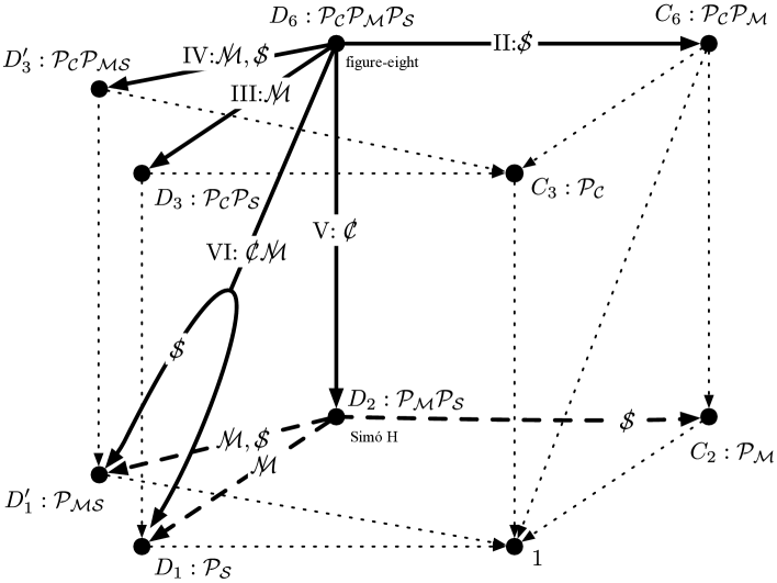
Figure 1: Bifurcations and symmetry breaking of $D_{6}$ and $D_{2}$. Bifurcations of $D_{6}$ and $D_{2}$ are represented by thick arrows and dashed thick arrows respectively. Each vertex represents the solution of the equations of motion. The symbol “$G:\mathcal{P}$” at each vertex represents symmetry group $G$ and projection operator $\mathcal{P}$ for the solution. The symbol “No:$\not{\mathcal{O}}$” on the arrows represents the number of irreducible representation in table 1 and broken symmetry $\mathcal{O}$. The fork in VI shows that this bifurcation yields two bifurcated solutions, one with symmetry group $D_{1}$ and the other with $D^{\prime}_{1}$. The bifurcation I in table 1 is bifurcation of $D_{6}\to D_{6}$ which is omitted in this figure.

3.1 Representation I: $\mathcal{P_{C}}^{\prime}=\mathcal{M}^{\prime}=\mathcal{S}^{\prime}=1$

Irreducible representation I is characterized by $\mathcal{P_{C}}^{\prime}=\mathcal{M}^{\prime}=\mathcal{S}^{\prime}=1$, namely, eigenfunction $\phi$ has these eigenvalues that is the same as $q_{o}$. The representation for group elements are $\tilde{\mathcal{B}}=\tilde{\mathcal{S}}=1$. This representation is called identity representation or trivial representation.

Since all $\mathcal{C},\,\mathcal{M},\mathcal{S}$ are the symmetry for $\{\phi,q_{o},S\}$, the projection operator is

$$\mathcal{P}_{I}=\mathcal{P_{C}}\mathcal{P_{M}}\mathcal{P_{S}}.$$ (81)

Then by the corollary 1, a bifurcation occurs and the bifurcated solution $q_{b}$ has the same invariance $D_{6}$ as the original $q_{o}$. The bifurcation pattern by this representation is

$$D_{6}\to D_{6}.$$ (82)

Since there is no reason for $\braket{\phi^{3}}=0$, we can safely assume $A_{3}=\braket{\phi^{3}}\neq 0$. Then order 1 bifurcation described in (54), (55) and (56) occurs.

As stated in section 2.5, order $1$ bifurcation can describe a fold bifurcation or “both-sides” bifurcation. Since symmetry group for $q_{o}$ and $q_{b}$ is the same in this bifurcation, a fold bifurcation is suitable.

3.2 Representation II: $\mathcal{P_{C}}^{\prime}=\mathcal{M}^{\prime}=1$ and $\mathcal{S}^{\prime}=-1$

Irreducible representation II is characterized by $\mathcal{P_{C}}^{\prime}=\mathcal{M}^{\prime}=1$ and $\mathcal{S}^{\prime}=-1$, namely, $\phi$ has these eigenvalues. In this representation $\tilde{\mathcal{B}}=1$, and $\tilde{\mathcal{S}}=-1$. Since the symmetry for $\{\phi,q_{o},S\}$ are $\mathcal{C}$ and $\mathcal{M}$, the projection operator is

$$\mathcal{P}_{II}=\mathcal{P_{C}}\mathcal{P_{M}}.$$ (83)

By the corollary 1, a bifurcation occurs and the invariance of the bifurcated solution is $\mathcal{P}_{II}q_{b}=q_{b}$. Namely, the invariance of $q_{b}$ is

$$C_{6}=\{1,\mathcal{B},\mathcal{B}^{2},\dots,\mathcal{B}^{5}\}.$$ (84)

The symmetry for $\mathcal{S}$ is broken. Bifurcation pattern by this representation is

$$D_{6}\to C_{6}.$$ (85)

By $\mathcal{S}\phi=-\phi$ and the theorem 2, the reduced action is even function of $r$: $S_{LS}(-r)=S_{LS}(r)$. Therefore, $A_{2n+1}=0$ for $n\geq 1$. There is no reason for $A_{4}=0$, we assume $A_{4}\neq 0$. Therefore order 2 bifurcation described by (59), (60) and (61) occurs.

3.3 Representation III: $\mathcal{P_{C}}^{\prime}=1,\,\mathcal{M}^{\prime}=-1,\,\mathcal{S}^{\prime}=1$

Irreducible representation III is characterized by $\mathcal{P_{C}}^{\prime}=\mathcal{S}^{\prime}=1$ and $\mathcal{M}^{\prime}=-1$. In this representation $\tilde{\mathcal{B}}=-1$ and $\tilde{\mathcal{S}}=1$. Since the symmetry for $\{\phi,q_{o},S\}$ are $\mathcal{C}$ and $\mathcal{S}$, the projection operator is

$$\mathcal{P}_{III}=\mathcal{P_{C}}\mathcal{P_{S}}.$$ (86)

By the corollary 1, a bifurcation occurs and the invariance of $q_{b}$ is

$$D_{3}=\{1,\mathcal{C},\mathcal{C}^{2},\mathcal{S},\mathcal{S}\mathcal{C},\mathcal{S}\mathcal{C}^{2}\}.$$ (87)

The symmetry for $\mathcal{M}$ is broken. The bifurcation pattern is

$$D_{6}\to D_{3}.$$ (88)

Since $\mathcal{M}\phi=-\phi$, $S_{LS}(-r)=S_{LS}(r)$ and $A_{2n+1}=0$ for $n\geq 1$. Assuming $A_{4}\neq 0$, order 2 bifurcation described by (59), (60) and (61) occurs.

3.4 Representation IV: $\mathcal{P_{C}}^{\prime}=1,\,\mathcal{M}^{\prime}=\mathcal{S}^{\prime}=-1$

Irreducible representation IV is characterized by $\mathcal{P_{C}}^{\prime}=1,\,\mathcal{M}^{\prime}=\mathcal{S}^{\prime}=-1$. In this representation $\tilde{\mathcal{B}}=\tilde{\mathcal{S}}=-1$. Since the symmetry for $\{\phi,q_{o},S\}$ are $\mathcal{C}$ and $\mathcal{MS}$, the projection operator is

$$\mathcal{P}_{IV}=\mathcal{P_{C}}\mathcal{P_{MS}}.$$ (89)

By the corollary 1, a bifurcation occurs and invariance of $q_{b}$ is

$$D_{3}^{\prime}=\{1,\mathcal{C},\mathcal{C}^{2},\mathcal{MS},\mathcal{MS}\mathcal{C},\mathcal{MS}\mathcal{C}^{2}\}.$$ (90)

Here, ^′ is added to distinguish this dihedral group of 6 elements from $D_{3}$ in (87). The symmetry of both $\mathcal{M}$ and $\mathcal{S}$ are broken, while the symmetry of $\mathcal{MS}$ is unbroken.

Since $\mathcal{M}\phi=\mathcal{S}\phi=-\phi$, $S_{LS}(-r)=S_{LS}(r)$ and $A_{2n+1}=0$ for $n\geq 1$. Assuming $A_{4}\neq 0$, order 2 bifurcation described by (59), (60) and (61) occurs.

3.5 Representation V: $\mathcal{P_{C}}^{\prime}=0,\,\mathcal{M}^{\prime}=1$ and $\mathcal{S}^{\prime}=\pm 1$

Irreducible representation V is characterized by $\mathcal{P_{C}}^{\prime}=0,\,\mathcal{M}^{\prime}=1$ and $\mathcal{S}^{\prime}=\pm 1$. This is two dimensional representation with

$$\tilde{\mathcal{B}}=\left(\begin{array}[]{rr}\cos(2\pi/3)&-\sin(2\pi/3)\\ \sin(2\pi/3)&\cos(2\pi/3)\end{array}\right)\mbox{ and }\tilde{\mathcal{S}}=\left(\begin{array}[]{cc}1&0\\ 0&-1\end{array}\right).$$ (91)

Eigenvalue $\kappa$ has degeneracy $d=2$. Let the eigenfunction $\phi_{\pm}$ be the eigenfunction of $\mathcal{S}\phi_{\pm}=\pm\phi_{\pm}$. They have $\mathcal{P_{C}}^{\prime}=0$ and $\mathcal{M}^{\prime}=1$.

Since the symmetry for $\{\phi_{+},q_{o},S\}$ are $\mathcal{M}$ and $\mathcal{S}$, the projection operator for $\phi_{+}$ is

$$\mathcal{P}_{V+}=\mathcal{P_{M}}\mathcal{P_{S}}.$$ (92)

Note that this projection operator chooses $\phi_{+}$ and discards $\phi_{-}$: $\mathcal{P}_{V+}\phi_{+}=\phi_{+}$, $\mathcal{P}_{V+}\phi_{-}=0$. Therefore by the corollary 1, a bifurcation in subspace of $\mathcal{P}_{V+}=\mathcal{P_{M}}\mathcal{P_{S}}$ occurs. The broken symmetry is $\mathcal{C}$ and invariance of the bifurcated solution is

$$D_{2}=\{1,\mathcal{M},\mathcal{S},\mathcal{SM}\}.$$ (93)

The bifurcation pattern is

$$D_{6}\to D_{2}.$$ (94)

On the other hand, the symmetry for $\{\phi_{-},q_{o},S\}$ is only $\mathcal{M}$. Therefore, the projection operator is $\mathcal{P_{M}}$. Since $\mathcal{P_{M}}$ does not exclude $\phi_{+}$, subspace of $\mathcal{P_{M}}$ remains two-dimensional. So the corollary 1 doesn’t ensure a bifurcation in the direction of $\phi_{-}$. Indeed we can show that there is bifurcated solution in $\phi_{+}$ direction, whereas no bifurcated solution in $\phi_{-}$ direction, by explicitly calculating the reduced action $S_{LS}$.

Let $\phi(\theta)=\cos(\theta)\phi_{+}+\sin(\theta)\phi_{-}$, then as shown in B, the the reduced action is given by

$$S_{LS}(r,\theta)=\frac{\kappa}{2}r^{2}+\frac{A_{3}(0)}{3!}r^{3}\cos(3\theta)+\frac{A_{4}(0)}{4!}r^{4}+O(r^{5}),$$ (95)

$$\frac{A_{3}(0)}{3!}=\frac{1}{3!}\braket{\phi_{+}^{3}},$$ (96)

$$\frac{A_{4}(0)}{4!}=\frac{1}{4!}\braket{\phi_{+}^{4}}-\frac{1}{(2!)^{3}}\sum_{\alpha}\frac{\braket{\phi_{+}^{2}\psi_{\alpha+}}^{2}}{\lambda_{\alpha}},$$ (97)

where $\mathcal{S}\psi_{\alpha+}=\psi_{\alpha+}$. The reduced action $S_{LS}$ in $(x,y)$ plane is shown in figure 2, where $(x,y)$ are orthogonal coordinates defined by $x=r\cos(\theta)$ and $y=r\sin(\theta)$ as usual. Then $r\phi(\theta)=x\phi_{+}+y\phi_{-}$.

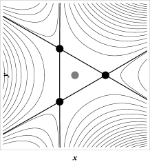
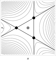
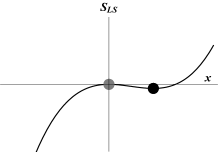
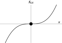
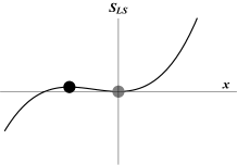
Figure 2: Reduced action $S_{LS}$ of representation V for $A_{3},A_{4}>0$. Upper: Contour plot of $S_{LS}$ in orthogonal coordinates $(x,y)$. Lower: $S_{LS}$ for $y=0$. From left to right $\kappa<0,\kappa=0$ and $\kappa>0$. Gray circle and black circles represent $q_{o}$ and $q_{b},\mathcal{C}q_{b},\mathcal{C}^{2}q_{b}$ respectively. For sufficiently small $\kappa$ and short range of $r$, terms of $O(r^{4})$ have no effect.

Note that $S_{LS}$ has the symmetry of regular triangle $D_{3}$, instead of $D_{6}$. The reason is $\mathcal{M}\phi(\theta)=\phi(\theta)$. By this invariance, the theorem 2 gives an identity: $S_{LS}(r,\theta)=S_{LS}(r,\theta)$. Therefore, $\mathcal{M}$ invariance is invisible in $S_{LS}$. On the other hand, $\mathcal{S}\phi(\theta)=\phi(-\theta)$, $\mathcal{C}\phi(\theta)=\phi(\theta+2\pi/3)$ and the theorem 2 give $S_{LS}(r,-\theta)=S_{LS}(r,\theta)$ and $S_{LS}(r,\theta\pm 2\pi/3)=S_{LS}(r,\theta)$ that show apparent invariance of $S_{LS}$ in $D_{3}$.

In other words, since quotient groups of $D_{6}$ and $D_{2}$ by the centre $\{1,\mathcal{M}\}$ are

$$D_{6}/\{1,\mathcal{M}\}\cong\{1,\mathcal{C},\mathcal{C}^{2},\mathcal{S},\mathcal{S}\mathcal{C},\mathcal{S}\mathcal{C}^{2}\}=D_{3}$$ (98)

$$D_{2}/\{1,\mathcal{M}\}\cong\{1,\mathcal{S}\}=D_{1},$$ (99)

this bifurcation pattern $D_{6}\to D_{2}$ that keeps $\mathcal{M}$ symmetry is equivalent to the bifurcation

$$D_{3}\to D_{1}.$$ (100)

This is the reason why the reduced action $S_{LS}$ has $D_{3}$ symmetry. The $D_{3}$ symmetry determines the form of $S_{LS}$ in (95).

The equations for stationary points are

$$\partial_{r}S_{LS}(r,\theta)=r\left(\kappa+\frac{A_{3}(0)}{2}r\cos(3\theta)+\frac{A_{4}(0)}{6}r^{2}+O(r^{3})\right)=0,$$ (101)

$$\partial_{\theta}S_{LS}=-\frac{A_{3}(0)}{2}r^{3}\sin(3\theta)+O(r^{5})=0.$$ (102)

The solutions are $r_{o}=0$ and

$$r_{b}=-\frac{2}{A_{3}(0)}\kappa-\frac{4A_{4}(0)}{3A_{3}(0)^{3}}\kappa^{2}+O(\kappa^{3}),\,\theta_{k}=\frac{2\pi}{3}k,\,k=0,1,2.$$ (103)

This is order 1 bifurcation. Let $q_{b}$ be the solution at $\theta=0$. Then

$$q_{b}=q_{o}+r_{b}\phi_{+}+r_{b}\sum_{\alpha}\epsilon_{\alpha}\psi_{\alpha},$$ (104)

with $\mathcal{P}_{V+}q_{b}=q_{b}$. Note that the solutions for $\theta$ in (103) are exact, namely, $O(r^{5})$ term in (102) does not change the solution $\theta$. Because of the $D_{3}$ symmetry of the reduced action, $\theta=0$ is exactly fixed. This is expected by the condition $\mathcal{P}_{V+}q_{b}=q_{b}$ in (92).

The solutions corresponds to $k=1,2$ are just copies of $q_{b}$: $\mathcal{C}^{k}q_{b}$. This is a direct result of $D_{3}$ symmetry of $S_{LS}(r,\theta)$. The symmetry by $\mathcal{S}$ does not make new solution, because $\mathcal{S}q_{b}=q_{b}$.

The action at the bifurcated solutions is

$$S_{LS}(r_{b},0)=S[q_{b}]-S[q_{o}]=\frac{2}{3A_{3}(0)^{2}}\kappa^{3}+\frac{2A_{4}}{3A_{3}(0)^{4}}\kappa^{4}+O(\kappa^{5})$$ (105)

and the second derivatives at the bifurcated solutions are $\left.r^{-1}\partial_{r}\partial_{\theta}S_{LS}\right|_{r=r_{b},\theta=0}=0$ and

$$\left.\partial_{r}^{2}S_{LS}(r,\theta)\right|_{r=r_{b},\theta=0}=\kappa+A_{3}(0)r_{b}+\frac{A_{4}(0)}{2}r_{b}^{2}+O(r_{b}^{3})=-\kappa+\frac{2A_{4}(0)}{3A_{3}(0)^{2}}\kappa^{2}+O(\kappa^{3}),$$ (106)

$$\left.r^{-2}\partial_{\theta}^{2}S_{LS}(r,\theta)\right|_{r=r_{b},\theta=0}=-\frac{3}{2}A_{3}(0)r_{b}+O(r_{b}^{3})=3\kappa+\frac{2A_{4}(0)}{A_{3}(0)}\kappa^{2}+O(\kappa^{3}).$$ (107)

Namely, the Hessian of the bifurcated solution has non-degenerate eigenvalues $-\kappa+O(\kappa^{2})$ and $3\kappa+O(\kappa^{2})$. Since $-\kappa$ and $3\kappa$ has opposite sign, the bifurcated solutions are saddle.

As stated in section 2.5, order $1$ bifurcation can describe fold bifurcation or “both-sides” bifurcation. Since, symmetry group for $q_{o}$ and $q_{b}$ are different and three copies $q_{b}$, $\mathcal{C}q_{b}$, $\mathcal{C}^{2}q_{b}$ exist, this bifurcation should be “both-sides”.

3.6 Representation VI: $\mathcal{P_{C}}^{\prime}=0,\,\mathcal{M}^{\prime}=-1$ and $\mathcal{S}^{\prime}=\pm 1$

This is another two dimensional representation with

$$\tilde{\mathcal{B}}=\left(\begin{array}[]{rr}\cos(\pi/3)&-\sin(\pi/3)\\ \sin(\pi/3)&\cos(\pi/3)\end{array}\right)\mbox{ and }\tilde{\mathcal{S}}=\left(\begin{array}[]{cc}1&0\\ 0&-1\end{array}\right).$$ (108)

This is the faithful representation of $D_{6}$. Let $\phi_{+}$ and $\phi_{-}$ be the eigenfunctions with $\mathcal{S}\phi_{\pm}=\pm\phi_{\pm}$. Then $\mathcal{P_{S}}\phi_{+}=\phi_{+}$ and $\mathcal{P_{S}}\phi_{-}=0$. Moreover, $\mathcal{P_{C}}\phi_{\pm}=\mathcal{P_{M}}\phi_{\pm}=0$. Note that the function $\phi_{-}$ has invariance $\mathcal{P_{MS}}\phi_{-}=\phi_{-}$, while $\mathcal{P_{MS}}\phi_{+}=0$.

The symmetry for $\{\phi_{+},q_{o},S\}$ is $\mathcal{S}$. Therefore, the projection operator is

$$\mathcal{P}_{VI+}=\mathcal{P_{S}}.$$ (109)

$\mathcal{P}_{VI+}$ excludes $\phi_{-}$: $\mathcal{P}_{VI+}\phi_{-}=0$. Therefore by the corollary 1, a bifurcation occurs for the direction of $\phi_{+}$ and invariance of $q_{b}$ is $\mathcal{P}_{VI+}=\mathcal{P_{S}}$. The broken symmetries are $\mathcal{C}$ and $\mathcal{M}$. Since $\braket{\phi_{+}^{3}}=0$ by $\mathcal{M}\phi_{+}=-\phi_{+}$, this bifurcation is order 2. The bifurcation pattern in this direction is

$$D_{6}\to D_{1}=\{1,\mathcal{S}\}.$$ (110)

We usually don’t say $D_{1}$, however, this notation is convenient for our purpose. See 5.2.3.

On the other hand, since the symmetry for $\{\phi_{-},q_{o},S\}$ is $\mathcal{MS}$, the projection operator for them is

$$\mathcal{P}_{VI-}=\mathcal{P_{MS}}.$$ (111)

Since $\mathcal{P}_{VI-}$ excludes $\phi_{+}$, by the corollary 1 a bifurcation occurs for the direction of $\phi_{-}$ and $q_{b}$ has invariance $\mathcal{P}_{VI-}=\mathcal{P_{MS}}$. The symmetry for $\mathcal{C}$, $\mathcal{M}$, and $\mathcal{S}$ are all broken, whereas the symmetry for $\mathcal{MS}$ remains. The bifurcation pattern in this direction is

$$D_{6}\to D_{1}^{\prime}=\{1,\mathcal{MS}\}.$$ (112)

Here, ^′ is used again to distinguish it from $D_{1}$ in (110). Since $\braket{\phi_{-}^{3}}=0$ by $\mathcal{M}\phi_{-}=-\phi_{-}$, this bifurcation is also order 2.

Therefore, at this bifurcation point, two order 2 bifurcations occur: one for $\phi_{+}$ direction with $\mathcal{P_{S}}$ invariance and another for $\phi_{-}$ direction with $\mathcal{P_{MS}}$ invariance. Let us denote them by $q_{b\pm}$:

$$q_{b\pm}=q_{o}+r_{b\pm}\phi_{\pm}+r_{b\pm}\sum_{\mathcal{P}_{VI\pm}\psi_{\alpha}=\psi_{\alpha}}\epsilon_{\alpha}(r_{b\pm},\theta_{\pm})\psi_{\alpha}.$$ (113)

Then a question arises. What is the relation between actions or second derivatives for one and another? To see this relation, let us calculate $S_{LS}$ in this subspace.

Let $\phi(\theta)=\cos(\theta)\phi_{+}+\sin(\theta)\phi_{-}$. Then the reduced action should be apparently invariant under the symmetry group $D_{6}$, because any element of $D_{6}$ change $\phi(\theta)$. Namely, $S_{LS}(r,\theta)$ is invariant under the transformations $\theta\to\theta+2\pi k/6$, $k=0,1,2,\dots,5$ and $\theta\to-\theta$. The $D_{6}$ invariance determines the form of $S_{LS}$ in the following:

$$S_{LS}(r,\theta)=\frac{\kappa}{2}r^{2}+\frac{A_{4}(0)}{4!}r^{4}+\frac{A_{6}(\theta)}{6!}r^{6}+O(r^{8}),$$ (114)

$$A_{6}(\theta)=A_{6+}\cos(3\theta)^{2}+A_{6-}\sin(3\theta)^{2},$$ (115)

where $A_{4}(0)$, $A_{6_{\pm}}$ are independent from $\theta$. The $\theta$ dependence of $S_{LS}(r,\theta)$ is very small because it appears in $r^{6}$ term. Parts of direct derivation for (114) are shortly shown in C. Figure 3 shows a typical behaviour of $S_{LS}$ in orthogonal coordinates $(x,y)=r(\cos\theta,\sin\theta)$.

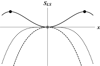
Figure 3: Reduced action $S_{LS}$ of representation VI for $A_{4}(0)<0,A_{6+}>A_{6-}>0$. Left: Contour plot of $S_{LS}$ for $\kappa>0$ in orthogonal coordinates $(x,y)$. Gray circle at the centre is $q_{0}$ and black circles and black stars are $\mathcal{B}^{k}q_{b+}$ and $\mathcal{B}^{k}q_{b-}$ with $k=0,1,2,\dots,5$ respectively. For this assignment of $A_{4}(0)$ and $A_{6\pm}$, $\mathcal{B}^{k}q_{b+}$ are local maximum and $\mathcal{B}^{k}q_{b-}$ are saddle. Right: $S_{LS}$ for $y=0$. Three curves represent $\kappa$ negative (dashed), zero (dotted) and positive(solid curve) respectively. For $A_{4}(0)<0$, bifurcated solutions $q_{b+}$ and $-q_{b+}$ (black circles) exist for $\kappa>0$. Gray circle at the origin is $q_{0}$.

The stationary points for $\theta$ are exactly given by

$$\theta_{+k}=\frac{2\pi}{6}k,\mbox{ and }\theta_{-k}=\frac{\pi}{2}+\frac{2\pi}{6}k\mbox{ with }k=0,1,2,\dots,5.$$ (116)

Let us write the solutions of $k=0$ as $\theta_{\pm}$ and $q_{b\pm}$, then the other solutions are copies of them: $\{q_{b+},\mathcal{B}q_{b+},\dots,\mathcal{B}^{5}q_{b+}\}$ and $\{q_{b-},\mathcal{B}q_{b-},\dots,\mathcal{B}^{5}q_{b-}\}$. For $\theta_{\pm}$, the reduced actions are

$$S_{LS}(r,\theta_{\pm})=\frac{\kappa}{2}r^{2}+\frac{A_{4}(0)}{4!}r^{4}+\frac{A_{6\pm}}{6!}r^{6}+O(r^{8}).$$ (117)

Then the stationary points in $r$ are $r=0$ and

$$r_{b+}=\pm\left(\frac{-6\kappa}{A_{4}(0)}\right)^{1/2}\left(1+\frac{3A_{6+}}{20A_{4}(0)^{2}}\kappa+O(\kappa^{2})\right),$$ (118)

$$r_{b-}=\pm\left(\frac{-6\kappa}{A_{4}(0)}\right)^{1/2}\left(1+\frac{3A_{6-}}{20A_{4}(0)^{2}}\kappa+O(\kappa^{2})\right).$$ (119)

Bifurcated solutions appear one-side, namely $\kappa>0$ if $A_{4}(0)<0$, or $\kappa<0$ if $A_{4}(0)>0$. They are order 2 bifurcations. The values of action at the bifurcated solutions are

$$S_{LS}(r_{b\pm},\theta_{\pm})=-\frac{3}{2A_{4}(0)}\kappa^{2}-\frac{3A_{6\pm}}{10A_{4}(0)^{3}}\kappa^{3}+O(\kappa^{4}).$$ (120)

The sign of the first term is the same as $\kappa$ because $\kappa$ and $A_{4}(0)$ have opposite signs. The difference of action between bifurcated solutions are small, because it appears in $\kappa^{3}$ term:

$$S_{LS}(r_{b+},\theta_{+})-S_{LS}(r_{b-},\theta_{-})=-\frac{3(A_{6+}-A_{6-})}{10A_{4}(0)^{3}}\kappa^{3}+O(\kappa^{4}).$$ (121)

Since $-\kappa^{3}/A_{4}(0)^{3}>0$, the sign of the difference is the same of that of $A_{6\pm}$. The second derivatives at bifurcated solutions are $r^{-1}\partial_{r}\partial_{\theta}S(r,\theta)|_{r_{b\pm},\theta_{\pm}}=0$ and

$$\partial_{r}^{2}S(r,\theta)|_{r_{b\pm},\theta_{\pm}}=-2\kappa+\frac{3A_{6\pm}}{5A_{4}(0)^{2}}\kappa^{2}+O(\kappa^{3}),$$ (122)

$$r^{-2}\partial_{\theta}^{2}S(r,\theta)|_{r_{b\pm},\theta_{\pm}}=\frac{9(A_{6\mp}-A_{6\pm})}{10A_{4}(0)^{2}}\kappa^{2}+O(\kappa^{3}).$$ (123)

The $\pm$ symbol in the last equation should be read $A_{6-}-A_{6+}$ for $\theta+$ and $A_{6+}-A_{6-}$ for $\theta-$. Namely $A_{6}$ for other minus $A_{6}$ for here. Since the main term of $\partial_{r}^{2}S_{LS}$ for $q_{b\pm}$ are common, while the main term of $r^{-2}\partial_{\theta}^{2}S_{LS}$ has opposite sign, one solution is a local minimum (if $A_{4}(0)>0$) or maximum (if $A_{4}(0)<0$), while the other is saddle.

4 Bifurcations of figure-eight solutions

A figure-eight solution has $D_{6}$ symmetry and bifurcation patterns of $D_{6}$ are already described in section 3 based only on the algebraic structure of the group, where the underlying symmetries for $\mathcal{B}$ and $\mathcal{S}$ have no meanings. In this section, we describe the contents of the symmetry of bifurcated solutions for figure-eight solutions.

Obviously, the symmetry $\mathcal{C}=\sigma^{-1}R^{1/3}$ describes choreographic symmetry. Other symmetry described by $\mathcal{M}$, $\mathcal{S}$ and $\mathcal{MS}$ is connected to geometric symmetries of locus of solutions. Here, locus is defined by neglecting time and exchange of particles. Then, $\mathcal{M}=\mu_{x}R^{1/2}$ is connected to $Y$-axis symmetry, $\mathcal{S}=-\tau\Theta$ to point symmetry around the origin, and $\mathcal{MS}=-\mu_{x}\tau R^{1/2}\Theta$ to $X$-axis symmetry.

Based on bifurcation patterns of $D_{6}$ described in section 3, bifurcations of figure-eight solutions are summarized in the table 2. The orbit of solution bifurcated at $a=-0.2142$ under $U_{h}$ is shown in figure 4. All other orbits are shown in [7]. Each bifurcation pattern yields each bifurcated solution with different choreographic and geometrical symmetry. The bifurcated solution by bifurcation V is Simó’s H solution [21]. The bifurcation V and VI was found by Muñoz-Almaraz et al. in 2006 [16] and confirmed by the present authors [7]. Bifurcations I to IV are found by the present authors [7]. Numerical calculations show that correspondence between parameter $\xi$ and $\kappa$ is one to two for I, while one to one for II to VI bifurcations. Therefore, order 1 bifurcation in I is surely fold while in V is “both-sides”, and order 2 bifurcations in II, III, IV and VI are “one-side” as expected.

Table 2: Bifurcation patterns of figure-eight solutions characterized by $\mathcal{P_{C}}^{\prime}$, $\mathcal{M}^{\prime}$, and $\mathcal{S}^{\prime}$ of the eigenfunction of Hessian $\mathcal{H}$. The column $d$ represents degeneracy number or dimensions for the representation. Symmetry represents the symmetry of the bifurcated solution. The last column describes the type of bifurcation, fold, one-side, or both-sides. The bifurcated solution in I to IV are choreographic, and V to VI are non-choreographic.

Pattern	$\mathcal{P_{C}}^{\prime}$	$\mathcal{M}^{\prime}$	$\mathcal{S}^{\prime}$	$d$	$a$ for $U_{h}$	$T$ for $U_{LJ}$		Symmetry	Type
						$\alpha_{-}$	$\alpha_{+}$
I	1	1	1	1		14.479	14.479	$X$- and $Y$-axis	fold
II	1	1	$-1$	1			17.132	$Y$-axis	one-side
III	1	$-1$	1	1			18.615	$O^{\rm b}$	one-side
IV	1	$-1$	$-1$	1	$-0.2142$	14.595		$X$-axis	one-side
V	0	1	$\pm 1$	2	0.9966	14.836	16.878	$X$- and $Y$-axis	both-sides
VI	0	$-1$	$\pm 1$	2	1.3424	14.861	16.111	$O^{\rm b}$ ora $X$-axis	doublea one-side

^a The bifurcation VI yields two kind of bifurcated solutions with different symmetry: $O$ symmetric one or $X$-axis symmetric one.
^b Symbol $O$ represents point symmetry around the origin.

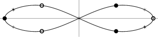
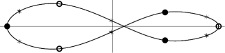
Figure 4: The figure-eight (left) and bifurcated solution for IV (right) under $U_{h}$ at $a=-0.2$. Points represent position of particles at $t=-T/12$ (solid circles), $0$ (black stars), $T/12$ (hollow circles), and $2T/12$ (grey stars).

Bifurcation in I is fold bifurcation between $\alpha_{\pm}$ solutions in $U_{LJ}$.

Bifurcations in II to IV are “one-side” bifurcations that yields “less symmetric eights”, namely choreographic solutions with less symmetry. Existence of “less symmetric eights” were predicted by Alain Chenciner [1, 2]. They surely exist in $U_{h}$ and $U_{LJ}$. The bifurcation at $a=-0.2142$ in $U_{h}$ is a bifurcation of pattern IV that yields choreographic solution that looses $Y$-axis symmetry and keeps $X$-axis symmetry. However, this branch does not reach $a=1$. The orbit of the bifurcated solution at $a=-0.2$ is shown in figure 4.

Bifurcated solution in IV has projection operator $\mathcal{P}_{IV}=\mathcal{P_{C}}\mathcal{P_{MS}}$, and one of the bifurcated solution in VI has $\mathcal{P}_{VI-}=\mathcal{P_{MS}}$. They have non-vanishing angular momentum. The reason is the following. In these bifurcations both $\mathcal{M}$ symmetry and $\mathcal{S}$ symmetry are broken. As a result, the bifurcated solution looses both $Y$-axis symmetry and the point symmetry around the origin. Then the total signed area has non-vanishing value which is equal to $T$ times of angular momentum $c$:

$$cT=\int_{0}^{T}dt\sum_{k=0,1,2}r_{k}\times\frac{dr_{k}}{dt}\neq 0.$$ (124)

Therefore, these bifurcated solutions have non-vanishing angular momentum. See figure 4.

Note that there are no direct paths $D_{6}\to C_{2}=\{1,\mathcal{M}\}$ that would produce non-choreographic solution with $Y$-axis symmetry and without $X$-axis symmetry. One possible path is cascading bifurcation via Simó’s H: $D_{6}\to D_{2}\to C_{2}$. Another one is $D_{6}\to C_{6}\to C_{2}$. See figure 1.

5 Summary and discussions

We applied group theoretical method in bifurcation to investigate bifurcations of periodic solutions in Lagrangian system. The results are summarized in the table 1, 2, 3 and the figure 1. In this method, bifurcated solution is a stationary point of the action. The second derivative of the action, Hessian $\mathcal{H}$, has important role. A non-trivial zero of the eigenvalue of Hessian yields bifurcation. Since eigenvalues and eigenfunctions are classified by irreducible representations of the symmetry of the Hessian, group theories have important role in bifurcations. In this method, symmetry breaking pattern and symmetry of bifurcated solution for each bifurcation is clear. Symmetry of Lyapunov-Schmidt reduced action apparently shows existence of the bifurcated solutions. This method will give an alternative method to analyse bifurcations of periodic solutions, although this method will be mathematically equivalent to methods based on Poincaré map or Floquet matrix.

5.1 Bifurcations of figure-eight solutions and Simó’s H

This method gives theoretical explanations to numerically obtained bifurcations of figure-eight solutions under $U_{h}$ with parameter $a$ and $U_{LJ}$ with parameter $T$ in the unified way. The results are summarized in table 2.

This method also predicts patterns for bifurcations of Simó’s H that has symmetry group $D_{2}$. Since $D_{2}$ is Abelian, it has 4 one-dimensional irreducible representations, which are characterized by $\mathcal{M}^{\prime}=\pm 1$ and $\mathcal{S}^{\prime}=\pm 1$. The bifurcation patterns are obvious that are summarized in table 3 and figure 1.

Table 3: Four irreducible representations of Group $D_{2}$ characterized by $\mathcal{M}^{\prime}$ and $\mathcal{S}^{\prime}$. All representations are one-dimensional ($d=1$). The next two columns represent projection operators $\mathcal{P}$ and symmetry group $G$ for the bifurcated solution. The order represents order $n$ of the bifurcation: $\kappa=-A_{n+2}\,r^{n}/(n+1)!+O(r^{n+1}),\,A_{n+2}\neq 0$. The last column describes the type of bifurcation.

• Representation	$\mathcal{M}^{\prime}$	$\mathcal{S}^{\prime}$	$d$	$\mathcal{P}$	$G$	Order	Type
  I′	1	1	1	$\mathcal{P_{M}}\mathcal{P_{S}}$	$D_{2}$	1	folda
  II′	1	$-1$	1	$\mathcal{P_{M}}$	$C_{2}$	2	one-side
  III′	$-1$	1	1	$\mathcal{P_{S}}$	$D_{1}$	2	one-side
  IV′	$-1$	$-1$	1	$\mathcal{P_{MS}}$	$D_{1}^{\prime}$	2	one-side

• ^aFold bifurcation is suitable, although both-sides is still possible.

Galán et al. [8] takes $m_{0}$ as a parameter. In this case, $m_{0}\neq 1$ breaks $\sigma$ symmetry $\sigma(r_{0},r_{1},r_{2})=(r_{1},r_{2},r_{0})$, while $\tau$ symmetry $\tau(r_{0},r_{1},r_{2})=(r_{0},r_{2},r_{2})$ is preserved. Then, the symmetry group for the figure-eight solution is reduced into $D_{2}$. This is the symmetry group for Simó’s H solution. Therefore, $D_{2}\to D_{2}$ bifurcation in table 3 connects the figure-eight solution and Simó’s H by fold bifurcation [8].

5.2 Group theoretical bifurcation theory

5.2.1 Existence of at least one bifurcated solution in each irreducible representation in $D_{n}$.

The arguments in section 2.6 show that at least one bifurcated solution exists in each irreducible representations. Actually, as shown above, each irreducible representations of $D_{6}$ has at least one projection operator that picks up one direction of corollary 1. Therefore, each irreducible representation has at least one bifurcated solution. This is also true for $D_{n}$, namely, there is at least one projection operator such that $\mathcal{P}q_{o}=q_{o}$ and $\mathcal{P}\phi(\theta)=\phi(\theta)$ (one dimension) for each irreducible representation. A proof is the following: It is known that the dimension of each irreducible representation of $D_{n}$ is one or two. (For odd $n$: 2 one-dimensional representations and $(n-1)/2$ two-dimensional ones. For even $n$: 4 one-dimensional and $n/2-1$ two-dimensional ones.) In two-dimensional representation, the degeneracy comes from two eigenfunctions $\mathcal{S}\phi_{\pm}=\pm\phi_{\pm}$ with definition $\mathcal{S}q_{o}=q_{o}$. Therefore the projection operator in corollary 1 that has the form $\mathcal{P}=\mathcal{P}\mathcal{P_{S}}\neq 0$ always exists, which picks up $\phi_{+}$ and excludes $\phi_{-}$. This is the projection operator we are looking for.

5.2.2 Similarity of bifurcation patterns.

As shown in this paper, the bifurcation patterns depend only on the group structure of symmetry group $G$ for the original solution $q_{o}$ and the action $S$. Therefore, if two different systems have symmetry groups $G$ and $G^{\prime}$, and $G$ and $G^{\prime}$ are isomorphic or homomorphic, the bifurcation patterns of the two systems are the same or similar.

For example. the bifurcation patterns I to IV of $D_{6}$ in table 1 and I^′ to IV^′ of $D_{2}$ in table 3 is similar if we neglect $\mathcal{P_{C}}$ in column $\mathcal{P}$ in the former table. The reason is the following. In bifurcation patterns I to IV of $D_{6}$, the symmetry of $\mathcal{C}$ is kept. Since $\{1,\mathcal{C},\mathcal{C}^{2}\}$ is a normal subgroup of $D_{6}$, we can make quotient group:

$$D_{6}/\{1,\mathcal{C},\mathcal{C}^{2}\}\cong\{1,\mathcal{M},\mathcal{S},\mathcal{S}\mathcal{M}\}=D_{2}.$$ (125)

Therefore, bifurcations of $D_{6}$ keeping $\mathcal{C}$ symmetry are equivalent to bifurcations of $D_{2}$.

In the next sub-subsection, we consider cases where two completely different system having isomorphic symmetry groups.

5.2.3 Period $k$ bifurcation.

Consider period $k$ bifurcations of a figure-eight solution. For this case, the periodic condition for an variation $\delta q(t)$ should be

$$\delta q(t+kT)=\delta q(t),$$ (126)

where $T$ is the period of this figure-eight solution. That means $\mathcal{B}^{6k}=\mathcal{R}^{k}=1$, instead of $\mathcal{B}^{6}=\mathcal{R}=1$. Therefore, the symmetry group is

$$D_{6k}=\{1,\mathcal{B},\dots,\mathcal{B}^{6k-1},\mathcal{S},\mathcal{S}\mathcal{B},\dots,\mathcal{S}\mathcal{B}^{6k-1}\},\,\mathcal{B}\mathcal{S}=\mathcal{S}\mathcal{B}^{-1}.$$ (127)

For example, period $k=5$ bifurcation will be determined by irreducible representations of $D_{30}$. Some of $k=5$ slalom solutions by M. Šuvakov and V. Dmitrašinović [22, 24], and M. Šuvakov and M. Shibayama [23] will turn out to be bifurcated solutions of the figure-eight by period 5 bifurcation.

Similarly, period $3$ bifurcations of Simó’s H ($D_{2}=\{1,\mathcal{M},\mathcal{S},\mathcal{S}\mathcal{M}\}$) will be described as bifurcation of

$$D_{6}^{\prime}=\{1,\mathcal{M},\mathcal{M}^{2},\dots,\mathcal{M}^{5},\mathcal{S},\mathcal{S}\mathcal{M},\mathcal{S}\mathcal{M}^{2},\dots,\mathcal{S}\mathcal{M}^{5}\}\cong D_{6},$$ (128)

because $\mathcal{M}^{6}=\mathcal{R}^{3}=1$ for period 3 bifurcation. Namely, it must have the same bifurcation patterns in table 1 and figure 1. Moreover, period $2$ of $D_{3}$ or period $6$ of $D_{1}$ bifurcation will be described by $D_{6}$.

Consider a periodic solution that is invariant under an operator $\mathcal{S}=\mathcal{O}\Theta$ where $\Theta$ is the time reversal and $\mathcal{O}$ satisfies $(\mathcal{O}\Theta)^{2}=1$, $\mathcal{O}\mathcal{R}=\mathcal{R}\mathcal{O}$. A simple example for $\mathcal{O}$ is $\mathcal{O}=-1$. In this case, $\mathcal{S}q_{o}=q_{o}$ means $q_{o}(-t)=-q_{o}(t)$. In general, assuming $q_{o}$ has no other invariance, the symmetry group for $q_{o}$ and $S$ is $D_{1}=\{1,\mathcal{S}\}$. Then, period $k$ bifurcation of this solution will be described by the dihedral group of regular $k$-gon,

$$D_{k}^{\prime}=\{1,\mathcal{R},\dots,\mathcal{R}^{k-1},\mathcal{S},\mathcal{S}\mathcal{R},\dots,\mathcal{S}\mathcal{R}^{k-1}\},\,\mathcal{R}\mathcal{S}=\mathcal{S}\mathcal{R}^{-1}.$$ (129)

For example, period doubling bifurcation of this system should be described by bifurcation of $D_{2}$, and period 3 bifurcation by $D_{3}$, and period 6 bifurcation by $D_{6}$. Indeed, in the book of K. R. Meyer and G. R. Hall [12] or Meyer and D. C. Offin [13], they describe period doubling, period 3 and period 6 bifurcations for Hamiltonian system that are exactly expected for bifurcations in faithful representation of $D_{2}$ (pattern IV or IV^′ in this paper), $D_{3}$ (pattern V) and $D_{6}$ (pattern VI), although we don’t consider the stability of original and bifurcated solution(s) here. See sections “Period doubling” and “$k$-bifurcation points” in [12] or [13].

For $k=2$, $D_{2}^{\prime}$ is

$$D_{2}^{\prime}=\{1,\mathcal{R},\mathcal{S},\mathcal{SR}\}.$$ (130)

The faithful representation is $\tilde{\mathcal{R}}=\tilde{\mathcal{S}}=-1$. Therefore bifurcation pattern is

$$D_{2}^{\prime}\to\{1,\mathcal{RS}\}=D_{1}^{\prime\prime}.$$ (131)

Therefore, period doubling bifurcation should be order 2 bifurcation with bifurcated solution that satisfies $\mathcal{RS}q_{b}=q_{b}$ on one side of parameter. Two solutions $\{q_{b},\mathcal{S}q_{b}=\mathcal{R}q_{b}\}$ exist at one side of the bifurcation point.

The faithful representation of $D_{3}$ is

$$\mathcal{R}=\left(\begin{array}[]{rr}\cos(2\pi/3)&-\sin(2\pi/3)\\ \sin(2\pi/3)&\cos(2\pi/3)\end{array}\right),\,\mathcal{S}=\left(\begin{array}[]{cc}1&0\\ 0&-1\end{array}\right).$$ (132)

This is the same as the irreducible representation in pattern V. The symmetry breaking pattern in this bifurcation is

$$D_{3}^{\prime\prime}=\{1,\mathcal{R},\mathcal{R}^{2},\mathcal{S},\mathcal{S}\mathcal{R},\mathcal{S}\mathcal{R}^{2}\}\to D_{1}=\{1,\mathcal{S}\}.$$ (133)

Therefore, period 3 bifurcation should be order 1 with $\mathcal{S}q_{b}=q_{b}$. Three bifurcated solutions $\{q_{b},\mathcal{R}q_{b},\mathcal{R}^{2}q_{b}\}$ exist for both side of parameter.

The faithful representations of $D_{6}$ produce $D_{6}\to D_{1}\mbox{ or }D_{1}^{\prime}$ as shown in bifurcation pattern VI in this paper. Therefore period 6 bifurcation should be order 2 with two kinds of bifurcated solutions for one side of parameter. One satisfies $\mathcal{S}q_{1}=q_{1}$, and other satisfies $\mathcal{R}^{3}\mathcal{S}q_{2}=q_{2}$. Each of them has 6 copies $\{q_{1},\mathcal{R}q_{1},\dots,\mathcal{R}^{5}q_{1}\}$ and $\{q_{2},\mathcal{R}q_{2},\dots,\mathcal{R}^{5}q_{2}\}$.

5.2.4 Symmetry breaking of bifurcation and preserving of the action.

As shown in section 3, bifurcation in II to VI breaks a symmetry or symmetries. While, symmetry of action $S$ is always preserved. The Lyapunov-Schmidt reduced action $S_{LS}$ inherits this invariance. As a result, multiple copies of a bifurcated solution by the broken symmetry will emerge from the bifurcation point: $\{q_{b},gq_{b},g^{2}q_{b},\dots,g^{n_{g}-1}q_{b}\}$ where $g$ is a broken symmetry and $n_{g}$ is the order of $g$. The locus of copies are congruent.

For example, in bifurcation V, the bifurcated solution $q_{b}$ breaks $\mathcal{C}$ invariance, therefore the invariance of the action under the transformation $\mathcal{C}$ yields three solutions $\{q_{b},\mathcal{C}q_{b},\mathcal{C}^{2}q_{b}\}$ that have congruent locus. Similarly, the breaking of $\mathcal{M}$ yields two bifurcated solutions $\{q_{b},\mathcal{M}q_{b}\}$. It is the same for $\mathcal{S}$. Note that in the case both $\mathcal{M}$ and $\mathcal{S}$ are broken while $\mathcal{MS}$ is preserved, we still have two bifurcated solutions $\{q_{b},\mathcal{S}q_{b}=\mathcal{M}q_{b}\}$ with congruent locus, since the invariance $\mathcal{MS}q_{b}=q_{b}$ ensures $\mathcal{S}q_{b}=\mathcal{M}q_{b}$. Thus bifurcations in II to IV yield two bifurcated solutions with congruent locus. Similarly, bifurcation VI yields solutions in two congruent classes $\{q_{b+},\mathcal{B}q_{b+},\dots,\mathcal{B}^{5}q_{b+}\}$ and $\{q_{b-},\mathcal{B}q_{b-},\dots,\mathcal{B}^{5}q_{b-}\}$.

On the other hand, any unbroken symmetry is invisible. This is because if $g\phi(\theta)=\phi(\theta)$, the symmetry for the reduced action yields identity $S_{LS}(r,\theta)=S_{LS}(r,\theta)$ that has no information. Similarly, if $gq_{b}=q_{b}$, $g$ does not produce new solution.

5.3 Further investigations

5.3.1 Stability.

Until now, relations between the behaviour of the action around a solution and the stability of the solution is unclear. For this reason, we used terms “both-sides” or “one-side” instead of “trans-critical” or “pitchfork”. Actually, the bifurcation at $a=0.9966$ and $a=1.3424$ for $U_{h}$ does not change the stability of the figure-eight solution [16]. We confirmed their results. The stability change/unchanged at $a=-0.2142$ still needs careful investigations. As shown in 5.2.3, bifurcations of the figure-eight solution at $a=-0.2142,\,0.9966$ and $1.3424$ is equivalent, in a group theoretical point of view, to period 2, 3, and 6 bifurcations. We suspect this might be an origin of exotic behaviour of stability change at these points. So, further systematic and careful numerical investigations and theoretical developments for changing stability at bifurcation points with a group theoretical point of view are required.

5.3.2 Stationary point at finite distance.

To describe bifurcations, it is enough to consider infinitesimally small distance from the original periodic solution. Then the first non-zero $A_{n}$ in (53) determines the properties of each bifurcation. Can we predict the existence of other periodic solutions at finite distance from the derivatives at original?

To make the argument clear, take the figure-eight solution as an original one and consider the subspace selected by projection operator $\mathcal{P}=\mathcal{P_{M}}\mathcal{P_{S}}$, which is the subspace where Simó’s H solution lives. The reduced action is a function of one variable $r$:

$$S_{LS}(r)=\frac{\kappa}{2}r^{2}+\sum_{n\geq 3}\frac{A_{n}}{n!}r^{n}=\frac{\kappa}{2}r^{2}+\frac{A_{3}}{3!}r^{3}+\frac{A_{4}}{4!}r^{4}+\dots.$$ (134)

The term $A_{3}r^{3}/3!$ goes to $-\infty$ for either $r\to+\infty$ or $-\infty$. Now, consider what will happen if $A_{4}$ is positive or simply if $S_{LS}(r)$ goes to sufficiently large positive for a finite value of $r$. Then, there must be at least one more stationary point at a finite distance. By the theorem 1, any stationary point in this subspace is a solution of the equations of motion and the solution has the symmetry of Simó’s H: $\mathcal{P}=\mathcal{P_{M}}\mathcal{P_{S}}$. Such solution surely exists near the figure-eight and Simó’s H solutions. Munõz-Almaraz et al. [16] showed numerically that Simó’s H solution has fold bifurcations at the both end of a interval of $a$. Therefore, near the end of this interval, the figure-eight, Simó’s H and one other solution exist. Then at the end of the interval, Simó’s H and the other solution are pair-annihilated by fold bifurcation. The present authors confirmed their results numerically.

Similar question also arises for bifurcation pattern VI. Numerical calculations for $U_{h}$ show that the bifurcated solutions emerge in $\kappa>0$ side. This means $A_{4}(0)<0$. Then if $A_{6\pm}>0$ or if $S_{LS}$ becomes sufficiently large positive for a finite value of $r$, then at least another solution exists at finite distance.

Can we theoretically treat the figure-eight solution, bifurcated solution(s) and solution(s) at finite distance at once, and can describe the observed fold bifurcations? It will be very interesting if we can do it by considering the behaviour of action around the figure-eight solution.

5.3.3 Equality of the second derivatives of $S_{LS}(r,\theta)$ and the eigenvalues of Hessian at $q_{b}$.

We have shown in appendix D that the second derivative of the reduced action at $q_{b}$ is equal to corresponding eigenvalues of Hessian at $q_{b}$ to order $r^{2}$ using ordinary perturbation method for the eigenvalues. However, the interesting term in (123) is of order $r^{4}$. So, equality to order $r^{2}$ is not enough for bifurcation VI. Since ordinary perturbation methods are tedious and inefficient, we need to find efficient methods to show equality or inequality of them.

Appendix A Proof of inheritance of symmetry

In this section, we will prove the equalities in section 2.8.

A proof of lemma 1 is the followings;

Proof.

Since $G$ is a symmetry group for $q_{o}$ and $S$, for arbitrary variation $\delta q$, we have

$$S[q_{o}+\delta q]=S[q_{o}+g\delta q].$$ (135)

Expansions of the action around $q_{o}$ yields

$$\frac{1}{2}\int dt\,\delta q\mathcal{H}\delta q+\sum_{n\geq 3}\frac{1}{n!}\braket{\delta q^{n}}=\frac{1}{2}\int dt\,(g\delta q)\mathcal{H}(g\delta q)+\sum_{n\geq 3}\frac{1}{n!}\braket{(g\delta q)^{n}}.$$ (136)

Since, $\delta q$ is arbitrary function, this equation holds for order by order:

$$\int dt\,\delta q\mathcal{H}\delta q=\int dt\,(g\delta q)\mathcal{H}(g\delta q),$$ (137)

$$\braket{\delta q^{n}}=\braket{(g\delta q)^{n}}.$$ (138)

So, if we take $\delta q=a_{i}e_{i}+a_{j}e_{j}$, we get

$$\int dt\,(ge_{i})\mathcal{H}(ge_{j})=\int dt\,e_{i}\mathcal{H}e_{j}=\lambda_{i}\delta_{ij}.$$ (139)

Where $\lambda_{i}$ is the eigenvalue of $\mathcal{H}$ for $e_{i}$. Moreover, if we put $\delta q=a_{i}e_{i}+a_{j}e_{j}+\dots$ into (138) and compare the corresponding term $a_{i}\vphantom{)}^{n_{i}}a_{j}\vphantom{)}^{n_{j}}\dots$ of left and right side, we get the lemma 1. ∎

Next, let us prove the theorem 2.

Proof.

The definition of $S_{LS}(r,\theta)$ and the invariance of action under $g$ yields

$$S_{LS}(r,\theta) =S\left[q_{o}+r\phi(\theta)+r\sum_{\alpha}\epsilon_{\alpha}(r,\theta)\psi_{\alpha})\right]$$ (140)

$$=S\left[q_{o}+r^{\prime}\phi(\theta^{\prime})+r\sum_{\alpha}\epsilon_{\alpha}(r,\theta)g\psi_{\alpha})\right].$$ (141)

So, if

$$r\epsilon_{\alpha}(r,\theta)g\psi_{\alpha}=r^{\prime}\epsilon_{\alpha}(r^{\prime},\theta^{\prime})\psi_{\alpha}$$ (142)

is satisfied, (79) is satisfied. Where $r^{\prime}\epsilon_{\alpha}(r^{\prime},\theta^{\prime})$ is the solution of (44) for $r^{\prime}\phi(\theta^{\prime})$. Therefore our goal is to show that $r^{\prime}\epsilon_{\alpha}(r^{\prime},\theta^{\prime})$ in (142) surely satisfies (44) for $r^{\prime}\phi(\theta^{\prime})$. This is true, because $\epsilon_{\alpha}$ in (44) is the unique solution for $r$ and $\phi(\theta)$ including the sign. However, a direct proof will be interesting.

Now, let us show this. For each $\psi_{\alpha}$, there is an orthogonal matrix representation $\tilde{g}_{\alpha}$ of $g$,

$$g\psi_{\alpha}=\psi_{\alpha}\tilde{g}_{\alpha}.$$ (143)

If $\psi_{\alpha}$ belongs one-dimensional representation, $\tilde{g}_{\alpha}=\pm 1$. If $\psi_{\alpha}$ belongs two-dimensional representation, $\tilde{g}_{\alpha}$ is a 2 by 2 matrix: for $s=\pm$,

$$g\psi_{\alpha s}=\sum_{s^{\prime}=\pm 1}\psi_{\alpha s^{\prime}}\tilde{g}_{\alpha s^{\prime},\alpha s},\mbox{ and }\sum_{s=\pm}\tilde{g}_{\alpha s^{\prime},\alpha s}\tilde{g}_{\alpha s^{\prime\prime},\alpha s}=\delta_{s^{\prime},s^{\prime\prime}}.$$ (144)

Let us start from the definition (44) of $\epsilon_{\alpha}(r,\theta)$. Then the invariance of integrals under $g$ yields

$$r\epsilon_{\alpha s}(r,\theta)=-\frac{1}{\lambda_{\alpha}}\sum_{n\geq 3}\frac{1}{(n-1)!}\Braket{\left(rg\phi(\theta)+r\sum_{\beta}\epsilon_{\beta}(r,\theta)g\psi_{\beta}\right)^{n-1}g\psi_{\alpha s}}$$

$$=-\frac{1}{\lambda_{\alpha}}\sum_{n\geq 3}\frac{1}{(n-1)!}\Braket{\left(r^{\prime}\phi(\theta^{\prime})+r\sum_{\beta}\psi_{\beta}\tilde{g}_{\beta}\epsilon_{\beta}(r,\theta)\right)^{n-1}\sum_{s^{\prime}=\pm}\psi_{\alpha s^{\prime}}\tilde{g}_{\alpha s^{\prime},\alpha s}},$$ (145)

where $\psi_{\beta}\tilde{g}\epsilon_{\beta}$ is the matrix notation for

$$\psi_{\beta}\tilde{g}_{\beta}\epsilon_{\beta}=\sum_{s^{\prime},s^{\prime\prime}=\pm}\psi_{\beta s^{\prime}}\tilde{g}_{\beta s^{\prime},\beta s^{\prime\prime}}\epsilon_{\beta s^{\prime\prime}}.$$ (146)

Therefore,

$$r(\tilde{g}_{\alpha}\epsilon_{\alpha}(r,\theta))_{s^{\prime\prime}}=r\sum_{s=\pm}\tilde{g}_{\alpha s^{\prime\prime},\alpha s}\epsilon(r,\theta)_{\alpha s}$$

$$=-\frac{1}{\lambda_{\alpha}}\sum_{n\geq 3}\frac{1}{(n-1)!}\Braket{\left(r^{\prime}\phi(\theta^{\prime})+r\sum_{\beta}\psi_{\beta}\tilde{g}_{\beta}\epsilon_{\beta}(r,\theta)\right)^{n-1}\sum_{s}\tilde{g}_{\alpha s^{\prime\prime},\alpha s}\sum_{s^{\prime}}\psi_{\alpha s^{\prime}}\tilde{g}_{\alpha s^{\prime},\alpha s}}$$

$$=-\frac{1}{\lambda_{\alpha}}\sum_{n\geq 3}\frac{1}{(n-1)!}\Braket{\left(r^{\prime}\phi(\theta^{\prime})+r\sum_{\beta}\psi_{\beta}\tilde{g}_{\beta}\epsilon_{\beta}(r,\theta)\right)^{n-1}\psi_{\alpha s^{\prime\prime}}}.$$ (147)

So, $r\tilde{g}_{\alpha}\epsilon_{\alpha}(r,\theta)$ satisfies the definition for $r^{\prime}\epsilon_{\alpha}(r^{\prime},\theta^{\prime})$. This is what we wanted to show. ∎

Appendix B $A_{k}(\theta)$, $k=3,4$ for V

In this section, we calculate $A_{k}(\theta)$, $k=3,4$ for bifurcation V. We use notation $\mathcal{S}\phi_{\pm}=\pm\phi_{\pm}$ and $\phi(\theta)=\cos(\theta)\phi_{+}+\sin(\theta)\phi_{-}$. We don’t need $\mathcal{M}$ operator for calculations in this section.

B.1 $A_{3}(\theta)$ for V

Expansion of $\phi(\theta)^{3}$ yields

$$\braket{\phi(\theta)^{3}}=\cos(\theta)^{3}\braket{\phi_{+}^{3}}+3\cos(\theta)\sin(\theta)^{2}\braket{\phi_{+}\phi_{-}^{2}},$$ (148)

because $\braket{\phi_{+}^{2}\phi_{-}}=\braket{\phi_{-}^{3}}=0$ by $\mathcal{S}\phi_{\pm}=\pm\phi_{\pm}$. Using the invariance of the lemma 1 for $g=\mathcal{B}$, we have $\braket{\phi_{+}^{3}}=\braket{(\mathcal{B}\phi_{+})^{3}}$ and $\braket{\phi_{+}\phi_{-}^{2}}=\braket{(\mathcal{B}\phi_{+})(\mathcal{B}\phi_{-})^{2}}$. On the other hand, $\phi_{\pm}$ are mixed by $\mathcal{B}$. Using the expression $\tilde{\mathcal{B}}$,

$$(\mathcal{B}\phi_{+},\mathcal{B}\phi_{-})=(\phi_{+},\phi_{-})\tilde{\mathcal{B}}=(\phi_{+},\phi_{-})\left(\begin{array}[]{rr}-1/2&-\sqrt{3}/2\\ \sqrt{3}/2&-1/2\end{array}\right)$$ (149)

Then, we have

$$\braket{\phi_{+}^{3}}=\braket{(\mathcal{B}\phi_{+})^{3}}=\Braket{\left(-\frac{1}{2}\phi_{+}+\frac{\sqrt{3}}{2}\phi_{-}\right)^{3}}=-\frac{1}{8}\braket{\phi_{+}^{3}}-\frac{9}{8}\braket{\phi_{+}\phi_{-}^{2}}.$$ (150)

Here we have used $\braket{\phi_{+}^{2}\phi_{-}}=\braket{\phi_{-}^{3}}=0$ again. Similar equation holds for $\braket{\phi_{+}\phi_{-}^{2}}=\braket{(\mathcal{B}\phi_{+})(\mathcal{B}\phi_{-})^{2}}$. Assembling two equations, we get the following equation:

$$\left(\begin{array}[]{l}\braket{\phi_{+}^{3}}\\ \braket{\phi_{+}\phi_{-}^{2}}\end{array}\right)=\left(\begin{array}[]{l}\braket{(\mathcal{B}\phi_{+})^{3}}\\ \braket{(\mathcal{B}\phi_{+})(\mathcal{B}\phi_{-})^{2}}\end{array}\right)=\left(\begin{array}[]{rr}-1/8&-9/8\\ -3/8&5/8\end{array}\right)\left(\begin{array}[]{l}\braket{\phi_{+}^{3}}\\ \braket{\phi_{+}\phi_{-}^{2}}\end{array}\right).$$ (151)

Namely, $(\braket{\phi_{+}^{3}},\braket{\phi_{+}\phi_{-}^{2}})$ must be an eigenvector of the matrix in the right side for eigenvalue 1. The solution is

$$\left(\begin{array}[]{l}\braket{\phi_{+}^{3}}\\ \braket{\phi_{+}\phi_{-}^{2}}\end{array}\right)=\left(\begin{array}[]{r}1\\ -1\end{array}\right)\braket{\phi_{+}^{3}}.$$ (152)

Substituting this solution into (148), we get

$$\braket{\phi(\theta)^{3}}=\left(\cos(\theta)^{3}-3\cos(\theta)\sin(\theta)^{2}\right)\braket{\phi_{+}^{3}}=\cos(3\theta)\braket{\phi_{+}^{3}}.$$ (153)

B.2 $A_{4}(\theta)$ for V

The invariance of integrals by $\phi_{\pm}\to\mathcal{B}\phi_{\pm}$ yields

$${\left(\begin{array}[]{l}\braket{\phi_{+}^{4}}\\ \braket{\phi_{+}^{2}\phi_{-}^{2}}\\ \braket{\phi_{-}^{4}}\end{array}\right)}={\left(\begin{array}[]{rrr}1/16&9/8&9/16\\ 3/16&-1/8&3/16\\ 9/16&9/8&1/16\end{array}\right)}{\left(\begin{array}[]{l}\braket{\phi_{+}^{4}}\\ \braket{\phi_{+}^{2}\phi_{-}^{2}}\\ \braket{\phi_{-}}^{4}\end{array}\right)}={\left({\begin{array}[]{c}1\\ 1/3\\ 1\end{array}}\right)}\braket{\phi_{+}^{4}}.$$ (154)

$$\therefore\braket{\phi(\theta)^{4}}=\cos(\theta)^{4}\braket{\phi_{+}^{4}}+6\cos(\theta)^{4}\sin(\theta)^{2}\braket{\phi_{+}^{2}\phi_{-}^{2}}+\sin(\theta)^{4}\braket{\phi_{-}^{4}}=\braket{\phi_{+}^{4}}.$$ (155)

Now, we proceed to calculate $\sum_{\alpha}\lambda_{\alpha}^{-1}\braket{\phi(\theta)^{2}\psi_{\alpha}}^{2}$;

$$\mbox{For }\mathcal{P_{C}}\psi_{\alpha+}=\psi_{\alpha+}\mbox{: }\left(\begin{array}[]{c}\braket{\phi_{+}^{2}\psi_{\alpha_{+}}}\\ \braket{\phi_{-}^{2}\psi_{\alpha_{+}}}\end{array}\right)=\left(\begin{array}[]{cc}1/4&3/4\\ 3/4&1/4\end{array}\right)\left(\begin{array}[]{c}\braket{\phi_{+}^{2}\psi_{\alpha_{+}}}\\ \braket{\phi_{-}^{2}\psi_{\alpha_{+}}}\end{array}\right)=\left(\begin{array}[]{c}1\\ 1\end{array}\right)\braket{\phi_{+}^{2}\psi_{\alpha_{+}}}.$$ (156)

$$\therefore\braket{\phi(\theta)^{2}\psi_{\alpha+}}=\cos(\theta)^{2}\braket{\phi_{+}^{2}\psi_{+}}+\sin(\theta)^{2}\braket{\phi_{-}^{2}\psi_{+}}=\braket{\phi_{+}^{2}\psi_{\alpha+}}.$$ (157)

$$\mbox{For }\mathcal{P_{C}}\psi_{\beta-}=\psi_{\beta-}\mbox{: }\braket{\phi_{+}\phi_{-}\psi_{\beta-}}=-\frac{1}{2}\braket{\phi_{+}\phi_{-}\psi_{\beta-}}=0.$$ (158)

$$\therefore\braket{\phi(\theta)^{2}\psi_{\beta-}}=2\cos(\theta)\sin(\theta)\braket{\phi_{+}\phi_{-}\psi_{\beta-}}=0.$$ (159)

$$\mbox{For }\mathcal{P_{C}}\psi_{\gamma\pm}=0\mbox{: }\left(\begin{array}[]{l}\braket{\phi_{+}^{2}\psi_{\gamma+}}\\ \braket{\phi_{-}^{2}\psi_{\gamma+}}\\ \braket{\phi_{+}\phi_{-}\psi_{\gamma-}}\end{array}\right) =\left(\begin{array}[]{rrr}-1/8&-3/8&\mp 3/4\\ -3/4&-1/8&\pm 3/4\\ \mp 3/8&\pm 3/8&1/4\end{array}\right)\left(\begin{array}[]{l}\braket{\phi_{+}^{2}\psi_{\gamma+}}\\ \braket{\phi_{-}^{2}\psi_{\gamma+}}\\ \braket{\phi_{+}\psi_{-}\psi_{\gamma-}}\end{array}\right)$$ (169)

$$=\left(\begin{array}[]{r}1\\ -1\\ -1\end{array}\right)\braket{\phi_{+}^{2}\psi_{\gamma+}},$$ (173)

where upper and lower sign represent the sign for $\psi_{\gamma}$ in representation V and in VI respectively. Therefore,

$$\braket{\phi(\theta)^{2}\psi_{\gamma+}}=\cos(\theta)^{2}\braket{\phi_{+}^{2}\psi_{\gamma+}}+\sin(\theta)^{2}\braket{\phi_{-}^{2}\psi_{\gamma+}}=\cos(2\theta)\braket{\phi_{+}^{2}\psi_{\gamma+}},$$ (174)

$$\braket{\phi(\theta)^{2}\psi_{\gamma-}}=2\cos(\theta)\sin(\theta)\braket{\phi_{+}\phi_{-}\psi_{\gamma-}}=-\sin(2\theta)\braket{\phi_{+}^{2}\psi_{\gamma+}},$$ (175)

$$\sum_{\mathcal{P_{C}}\psi_{\gamma}=0}\frac{1}{\lambda_{\gamma}}\left(\braket{\phi(\theta)^{2}\psi_{\gamma+}}^{2}+\braket{\phi(\theta)^{2}\psi_{\gamma-}}^{2}\right)=\sum_{\mathcal{P_{C}}\psi_{\gamma}=0}\frac{1}{\lambda_{\gamma}}\braket{\phi_{+}^{2}\psi_{\gamma+}}^{2}.$$ (176)

Assembling these terms, we get

$$\sum_{\alpha}\frac{1}{\lambda_{\alpha}}\braket{\phi(\theta)^{2}\psi_{\alpha}}^{2}=\sum_{\alpha}\frac{1}{\lambda_{\alpha}}\braket{\phi_{+}^{2}\psi_{\alpha+}}^{2}.$$ (177)

So, we get,

$$A_{4}(\theta)=\braket{\phi_{+}^{4}}-\sum_{\alpha}\frac{3}{\lambda_{\alpha}}\braket{\phi_{+}^{2}\psi_{\alpha+}}^{2}=A_{4}(0).$$ (178)

Appendix C $A_{k}(\theta)$, $k=3,4,5,6$ for VI

In this section, we calculate $A_{k}(\theta)$, $k=3,4,5,6$ for bifurcation VI.

C.1 $A_{3}(\theta),A_{5}(\theta),\dots$ for VI

By $\mathcal{M}\phi(\theta)=-\phi(\theta)$ and the theorem 2, The reduced action is an even function of $r$: $S_{LS}(r,\theta)=S_{LS}(-r,\theta)$. Therefore all $A_{2n+1}(r,\theta)=0$ for $n=1,2,\dots$. However, direct check will be interesting.

$A_{3}(\theta)=\braket{\phi(\theta)^{3}}=0$ is obvious by $\mathcal{M}\phi(\theta)=-\phi(\theta)$.

Three terms contribute to $A_{5}(\theta)$:

$$\braket{\phi(\theta)^{5}},\,\sum_{\alpha}\frac{\braket{\phi(\theta)^{2}\psi_{\alpha}}\braket{\phi(\theta)^{3}\psi_{\alpha}}}{\lambda_{\alpha}},\,\sum_{\alpha,\beta}\frac{\braket{\phi(\theta)^{2}\psi_{\alpha}}\braket{\phi(\theta)\psi_{\alpha}\psi_{\beta}}\braket{\phi(\theta)^{2}\psi_{\beta}}}{\lambda_{\alpha}\lambda_{\beta}}.$$ (179)

The first term is zero, because $\mathcal{M}\phi(\theta)=-\phi(\theta)$. The second term is zero, because $\braket{\phi^{2}\psi_{\alpha}}=0$ if $\mathcal{M}\psi_{\alpha}=-\psi_{\alpha}$, and $\braket{\phi^{3}\psi_{\alpha}}=0$ if $\mathcal{M}\psi_{\alpha}=\psi_{\alpha}$. For the last term, $\psi_{\alpha}$ and $\psi_{\beta}$ should belongs to $\mathcal{M}^{\prime}=1$ to give non-zero values to $\braket{\phi(\theta)^{2}\psi_{\alpha}}$ and $\braket{\phi(\theta)^{2}\psi_{\beta}}$. However, it gives $\braket{\phi(\theta)\psi_{\alpha}\psi_{\beta}}=0$. Therefore, the last term is also zero. So we get $A_{5}(r,\theta)=0$.

Therefore $\mathcal{M}\phi(\theta)=-\phi(\theta)$ surely ensure $A_{3}(\theta)=A_{5}(\theta)=0$ as predicted by the theorem 2.

C.2 $A_{4}(\theta)$ for VI

The term $A_{4}(\theta)$ has the same expression as in (178).

$$A_{4}(\theta)=\braket{\phi_{+}^{4}}-\sum_{\alpha}\frac{3}{\lambda_{\alpha}}\braket{\phi_{+}^{2}\psi_{\alpha+}}^{2}=A_{4}(0).$$ (180)

Because we can use $\mathcal{C}$ to calculate the relations between $\braket{\phi_{+}^{4}}$, $\braket{\phi_{+}^{2}\phi_{-}^{2}}$ and $\braket{\phi_{-}^{4}}$, etc., for example $\braket{\phi_{+}^{4}}=\braket{(\mathcal{C}\phi_{+})^{4}}$. Since the representation of $\mathcal{C}$ in VI is the same as that of $\mathcal{B}$ in V, we get the same relations in V.

C.3 $A_{6}(\theta)$ for VI

Seven terms contribute to $A_{6}(\theta)$: Here we pick up two simpler terms $\braket{\phi(\theta)^{6}}$ and $\sum\braket{\phi(\theta)^{3}\psi_{\alpha}}^{2}/\lambda_{\alpha}$. The invariance of integrals under $\phi_{\pm}\to\mathcal{C}\phi_{\pm}$ yields

$$\left(\begin{array}[]{l}\braket{\phi_{+}^{6}}\\ \braket{\phi_{+}^{4}\phi_{-}^{2}}\\ \braket{\phi_{+}^{2}\phi_{-}^{4}}\\ \braket{\phi_{-}^{6}}\end{array}\right)=\frac{1}{64}\left(\begin{array}[]{rrrr}1&45&135&27\\ 3&31&-27&9\\ 9&-27&31&3\\ 27&135&45&1\end{array}\right)\left(\begin{array}[]{l}\braket{\phi_{+}^{6}}\\ \braket{\phi_{+}^{4}\phi_{-}^{2}}\\ \braket{\phi_{+}^{2}\phi_{-}^{4}}\\ \braket{\phi_{-}^{6}}\end{array}\right).$$ (181)

There are two independent solutions

$$\left(\begin{array}[]{l}\braket{\phi_{+}^{6}}\\ \braket{\phi_{+}^{4}\phi_{-}^{2}}\\ \braket{\phi_{+}^{2}\phi_{-}^{4}}\\ \braket{\phi_{-}^{6}}\end{array}\right)=\left(\begin{array}[]{r}1\\ -2/5\\ 3/5\\ 0\end{array}\right)\braket{\phi_{+}^{6}}+\left(\begin{array}[]{r}0\\ 3/5\\ -2/5\\ 1\end{array}\right)\braket{\phi_{-}^{6}}.$$ (182)

$$\therefore\braket{\phi(\theta)^{6}} =\cos(\theta)^{6}\braket{\phi_{+}^{6}}+15\cos(\theta)^{4}\sin(\theta)^{2}\braket{\phi_{+}^{4}\phi_{-}^{2}}+15\cos(\theta)^{2}\sin(\theta)^{4}\braket{\phi_{+}^{2}\phi_{-}^{4}}\sin(\theta)^{6}\braket{\phi_{-}^{6}}$$ (183)

$$=\cos(3\theta)^{2}\braket{\phi_{+}^{6}}+\sin(3\theta)^{2}\braket{\phi_{-}^{6}}.$$

Now, let us proceed to calculate $\sum\braket{\phi(\theta)^{3}\psi_{\alpha}}^{2}/\lambda_{\alpha}$.

$$\mbox{For }\mathcal{P_{C}}\psi_{\alpha}=\psi_{\alpha}\mbox{: }\left(\begin{array}[]{r}\braket{\phi_{+}^{3}\psi_{\alpha+}}\\ \braket{\phi_{+}\phi_{-}^{2}\psi_{\alpha+}}\end{array}\right)=\left(\begin{array}[]{r}1\\ -1\end{array}\right)\braket{\phi_{+}^{3}\psi_{\alpha+}},$$ (188)

$$\left(\begin{array}[]{r}\braket{\phi_{+}^{2}\phi_{-}\psi_{\alpha-}}\\ \braket{\phi_{-}^{3}\psi_{\alpha-}}\end{array}\right)=\left(\begin{array}[]{rr}5/8&-3/8\\ -9/8&-1/8\end{array}\right)\left(\begin{array}[]{r}\braket{\phi_{+}^{2}\phi_{-}\psi_{\alpha-}}\\ \braket{\phi_{-}^{3}\psi_{\alpha-}}\end{array}\right)=\left(\begin{array}[]{c}-1\\ 1\end{array}\right)\braket{\phi_{-}^{3}\psi_{\alpha-}}.$$ (197)

$$\therefore\sum_{\mathcal{P_{C}}\psi_{\alpha}=\psi_{\alpha}}\!\!\!\!\!\!\frac{\braket{\phi(\theta)^{3}\psi_{\alpha}}^{2}}{\lambda_{\alpha}}={\left(\sum_{\mathcal{P_{C}}\psi_{\alpha+}=\psi_{\alpha+}}\!\!\!\!\!\!\frac{\braket{\phi_{+}^{3}\psi_{\alpha+}}^{2}}{\lambda_{\alpha}}\right)}\cos(3\theta)^{2}+{\left(\sum_{\mathcal{P_{C}}\psi_{\beta-}=\psi_{\beta-}}\!\!\!\!\!\!\frac{\braket{\phi_{-}^{3}\psi_{\beta-}}^{2}}{\lambda_{\beta}}\right)}\sin(3\theta)^{2}.$$ (198)

$$\mbox{For }\mathcal{P_{C}}\psi_{\alpha}=0\mbox{: }\left(\begin{array}[]{r}\braket{\phi_{+}^{3}\psi_{\alpha+}}\\ \braket{\phi_{+}\phi_{-}^{2}\psi_{\alpha+}}\\ \braket{\phi_{+}^{2}\phi_{-}\psi_{\alpha-}}\\ \braket{\phi_{-}^{3}\psi_{\alpha-}}\end{array}\right) =\frac{1}{16}\left(\begin{array}[]{rrrr}1&9&\pm 9&\pm 9\\ 3&-5&\pm 3&\pm 3\\ \pm 3&\pm 3&-5&3\\ \pm 9&\pm 9&9&1\end{array}\right)\left(\begin{array}[]{r}\braket{\phi_{+}^{3}\psi_{\alpha+}}\\ \braket{\phi_{+}\phi_{-}^{2}\psi_{\alpha+}}\\ \braket{\phi_{+}^{2}\phi_{-}\psi_{\alpha-}}\\ \braket{\phi_{-}^{3}\psi_{\alpha-}}\end{array}\right)$$ (211)

$$=\left(\begin{array}[]{c}1\\ 1/3\\ \pm 1/3\\ \pm 1\end{array}\right)\braket{\phi_{+}^{3}\psi_{\alpha+}},$$ (216)

where $\pm$ stands for the sign for $\psi_{\alpha}$ in representation VI and V respectively

$$\therefore\sum_{\mathcal{P_{C}}\psi_{\alpha}=0}\frac{\braket{\phi(\theta)^{3}\psi_{\alpha}}}{\lambda_{\alpha}}^{2}=\sum_{\mathcal{P_{C}}\psi_{\alpha}=0}\frac{1}{\lambda_{\alpha}}\left(\braket{\phi(\theta)^{3}\psi_{\alpha+}}^{2}+\braket{\phi(\theta)^{3}\psi_{\alpha-}}^{2}\right)=\sum_{\mathcal{P_{C}}\psi_{\alpha+}=0}\frac{\braket{\phi_{+}^{3}\psi_{\alpha+}}^{2}}{\lambda_{\alpha}},$$ (217)

which is $\theta$ independent.

Similarly, all terms in $A_{6}(\theta)$ contribute in the form $A_{6+}\cos(3\theta)^{2}+A_{6-}\sin(3\theta)^{2}$.

Appendix D The eigenvalue of Hessian at bifurcated solution

In this section, we calculate the eigenvalue of Hessian $\mathcal{H}$ at bifurcated solutions,

$$\mathcal{H}(q_{b})=\mathcal{H}(q_{o}+r\phi(\theta)+r\epsilon\psi)$$ (218)

by ordinary perturbation methods using the term $r\phi(\theta)+r\epsilon\psi$ for the perturbation term. Here, we used abbreviated notation $\epsilon\psi$ for

$$\epsilon\psi=\sum_{\alpha}\epsilon_{\alpha}\psi_{\alpha}.$$ (219)

Since we are considering a bifurcated solution $q_{b}=q_{o}+r\phi(\theta)+r\epsilon\psi$, $\phi(\theta)$ and $\epsilon\psi$ are filtered by a projection operator for this solution: $\mathcal{P}q_{b}=q_{b}$.

The zero order Hessian and the perturbation term are

$$\mathcal{H}(q_{o}+r\phi(\theta)+r\epsilon\psi)=\mathcal{H}(q_{o})+\Delta U,$$ (220)

$$\mathcal{H}(q_{o})=-\frac{d^{2}}{dt^{2}}+\frac{\partial^{2}U}{\partial q^{2}},$$ (221)

$$\Delta U=\mathcal{H}(q_{o}+r\phi(\theta)+r\epsilon\psi)-\mathcal{H}(q_{o})=\sum_{n\geq 1}\frac{r^{n}}{n!}(\phi(\theta)+\epsilon\psi)^{n}\frac{\partial^{n+2}U}{\partial q^{n+2}}.$$ (222)

For arbitrary functions $f$ and $g$,

$$\int dt\Delta Ufg=\sum_{n\geq 1}\frac{r^{n}}{n!}\braket{(\phi(\theta)+\epsilon\psi)^{n}fg}.$$ (223)

The aim of this section is to calculate the eigenvalue to order $r^{2}$. Since $\Delta U$ is order $r$, calculations to second order perturbation are enough.

D.1 Non-degenerate cases

For $\kappa$ is not degenerate, the ordinary perturbation method yields the eigenvalue of Hessian,

$$K =\kappa+\int dt\,\Delta U\phi^{2}-\sum_{\alpha}\frac{1}{\lambda_{\alpha}-\kappa}\left(\int dt\,\Delta U\phi\psi_{\alpha}\right)^{2}+O(\Delta U^{3})$$ (224)

$$=\kappa+r\braket{(\phi+\epsilon\psi)\phi^{2}}+\frac{r^{2}}{2}\braket{\phi^{4}}-\sum_{\alpha}\frac{r^{2}}{\lambda_{\alpha}}\braket{\phi^{2}\psi_{\alpha}}^{2}+O(r^{3}),$$

where we have used $O(\Delta U)=O(r)$, $\kappa=O(r)$ and $\epsilon=O(r)$. Using

$$\epsilon_{\alpha}=-\frac{1}{\lambda_{\alpha}}\sum_{n\geq 3}\frac{r^{n-2}}{(n-1)!}\braket{(\phi+\epsilon\psi)^{n-1}\psi_{\alpha}}=-\frac{r}{2\lambda_{\alpha}}\braket{\phi^{2}\psi_{\alpha}}+O(r^{2}),$$

we get

$$K=\kappa+r\braket{\phi^{3}}+\frac{r^{2}}{2}\left(\braket{\phi^{4}}-\sum_{\alpha}\frac{3}{\lambda_{\alpha}}\braket{\phi^{2}\psi_{\alpha}}^{2}\right)+O(r^{3}).$$ (225)

This is equal to $d^{2}S_{LS}(r)/dr^{2}$ of $S_{LS}(r)$ in (47).

D.2 Doubly degenerate cases

For bifurcations V and VI, the eigenvalue $\kappa$ is doubly degenerate. Let $\phi_{1}$ and $\phi_{2}$ be eigenfunctions for $\kappa$, $\phi_{1}$ be the function that contributes to the bifurcated function $q_{b}=q_{o}+\phi_{1}+\epsilon\psi$, and $\phi_{2}$ be another. Let $\mathcal{P}$ be the projection operator for $\mathcal{P}q_{b}=q_{b}$, then $\mathcal{P}\phi_{1}=\phi_{1}$ and $\mathcal{P}\phi_{2}=0$ follows. Here $\mathcal{P}$ is one of $\mathcal{P_{M}}\mathcal{P_{S}}$, $\mathcal{P_{S}}$, and $\mathcal{P_{MS}}$. Note that $\Delta U$ is diagonalised by $\phi_{1}$ and $\phi_{2}$:

$$\int dt\,\Delta U\phi_{1}\phi_{2}=\sum_{n}\frac{r^{n}}{n!}\braket{(\phi_{1}+\epsilon\psi)^{n}\phi_{1}\phi_{2}}=\sum_{n}\frac{r^{n}}{n!}\braket{(\phi_{1}+\epsilon\psi)^{n}\phi_{1}\mathcal{P}\phi_{2}}=0.$$ (226)

Here, we used the same arguments for the theorem 1. Then, the perturvative calculations are similar to that of non-degenerate cases to the second order:

$$K_{1}=\kappa+\int dt\Delta U\phi_{1}^{2}-\sum_{\alpha}\frac{1}{\lambda_{\alpha}-\kappa}\left(\int dt\,\Delta U\phi_{1}\psi_{\alpha}\right)^{2}+O(\Delta U^{3}),$$ (227)

$$K_{2}=\kappa+\int dt\Delta U\phi_{2}^{2}-\sum_{\alpha}\frac{1}{\lambda_{\alpha}-\kappa}\left(\int dt\,\Delta U\phi_{2}\psi_{\alpha}\right)^{2}+O(\Delta U^{3}).$$ (228)

Note that $\psi_{\alpha}$ in the second term of $K_{2}$ satisfies $\mathcal{P}\psi_{\alpha}=0$ because $\mathcal{P}\phi_{2}=0$ and $\Delta U$ is invariant.

D.2.1 For bifurcated solution in V.

For this case, $\mathcal{P}=\mathcal{P_{M}}\mathcal{P_{S}}$. Then $\phi_{1}=\phi_{+}$ and $\phi_{2}=\phi_{-}$, and $\epsilon\psi=\sum_{\alpha}\epsilon_{\alpha}\psi_{\alpha+}$ where $\mathcal{S}\phi_{\pm}=\pm\phi_{\pm}$ and $\mathcal{P_{S}}\psi_{\alpha+}=\psi_{\alpha+}$. Then,

$$\epsilon_{\alpha}=-\frac{r}{2\lambda_{\alpha}}\braket{\phi_{+}^{2}\psi_{\alpha+}}+O(r^{2}),$$ (229)

and

$$K_{1} =\kappa+\int dt\,\Delta U\phi_{+}^{2}-\sum_{\alpha}\frac{1}{\lambda_{\alpha}-\kappa}\left(\int dt\,\Delta U\phi_{+}\psi_{\alpha+}\right)^{2}$$ (230)

$$=\kappa+r\braket{\phi_{+}^{3}}+\frac{r^{2}}{2}\left(\braket{\phi_{+}^{4}}-\sum_{\alpha}\frac{3}{\lambda_{\alpha}}\braket{\phi_{+}^{2}\psi_{\alpha+}}^{2}\right)+O(r^{3}).$$

This is equal to $d^{2}S_{LS}(r)/dr^{2}$ of $S_{LS}(r)$ in (47). For $K_{2}$,

$$\int dt\,\Delta U\phi_{-}^{2}$$

$$=r\braket{\phi_{+}\phi_{-}^{2}}-\sum_{\alpha}\frac{r^{2}}{2\lambda_{\alpha}}\braket{\phi_{+}^{2}\psi_{\alpha+}}\braket{\phi_{-}^{2}\psi_{\alpha+}}+\frac{r^{2}}{2}\braket{\phi_{+}^{2}\phi_{-}^{2}}$$

$$=-r\braket{\phi_{+}^{3}}-\!\!\!\sum_{\mathcal{P_{C}}\psi_{\alpha+}=\psi_{\alpha+}}\frac{r^{2}}{2\lambda_{\alpha}}\braket{\phi_{+}^{2}\psi_{\alpha+}}^{2}+\!\!\!\sum_{\mathcal{P_{C}}\psi_{\beta+}=0}\frac{r^{2}}{2\lambda_{\beta}}\braket{\phi_{+}^{2}\psi_{\beta+}}^{2}+\frac{r^{2}}{6}\braket{\phi_{+}^{4}}+O(r^{3}).$$ (231)

Here we have used the relations in B.1 and B.2. On the other hand,

$$-\sum_{\alpha}\frac{1}{\lambda_{\alpha}-\kappa}\left(\int dt\,\Delta U\phi_{-}\psi_{\alpha-}\right)^{2}=-\sum_{\alpha}\frac{r^{2}}{\lambda_{\alpha}}\braket{\phi_{+}\phi_{-}\psi_{\alpha-}}^{2}+O(r^{3})$$

$$=-\sum_{\mathcal{P_{C}}\psi_{\alpha-}=0}\frac{r^{2}}{\lambda_{\alpha}}\braket{\phi_{+}^{2}\psi_{\alpha+}}^{2}+O(r^{3}).$$ (232)

Here, we have used (159) and (169). So, we get

$$K_{2} =\kappa-r\braket{\phi_{+}^{3}}-\!\!\!\!\!\sum_{\mathcal{P_{C}}\psi_{\alpha+}=\psi_{\alpha+}}\frac{r^{2}}{2\lambda_{\alpha}}\braket{\phi_{+}^{2}\psi_{\alpha+}}^{2}-\!\!\!\!\!\sum_{\mathcal{P_{C}}\psi_{\beta+}=0}\frac{r^{2}}{2\lambda_{\beta}}\braket{\phi_{+}^{2}\psi_{\beta+}}^{2}+\frac{r^{2}}{6}\braket{\phi_{+}^{4}}+O(r^{3})$$ (233)

$$=\kappa-r\braket{\phi_{+}^{3}}-\sum_{\alpha}\frac{r^{2}}{2\lambda_{\alpha}}\braket{\phi_{+}^{2}\psi_{\alpha+}}^{2}+\frac{r^{2}}{6}\braket{\phi_{+}^{4}}+O(r^{3})$$

$$=\kappa-A_{3}(0)r+\frac{A_{4}(0)}{3!}r^{2}+O(r^{3}).$$

Here we have used the relations in B.1 and B.2. Substituting $r=r_{b}$ in (103), we get the same expression as in (107).

D.2.2 For bifurcated solution in VI with $\mathcal{P}=\mathcal{P_{S}}$.

For this solution,

$$\phi_{1}=\phi_{+},\,\phi_{2}=\phi_{-},\,\epsilon\psi=\sum_{\alpha}\epsilon_{\alpha}\psi_{\alpha+},$$ (234)

$$\mathcal{P_{M}}\phi_{\pm}=0,$$ (235)

$$\epsilon_{\alpha}=-\frac{r}{2\lambda_{\alpha}}\braket{\phi_{+}^{2}\psi_{\alpha+}}.$$ (236)

Since, $\braket{\phi_{+}^{3}}=0$ by $\mathcal{M}\phi_{+}=-\phi_{+}$,

$$K_{1}=\kappa+\int dt\,\Delta U\phi_{+}^{2}-\sum_{\alpha}\frac{1}{\lambda_{\alpha}-\kappa}\left(\int dt\,\Delta U\phi_{+}\psi_{\alpha+}\right)^{2}+O(\Delta U^{3})$$

$$=\kappa+\frac{A_{4}(0)}{2}r^{2}+O(r^{3}).$$ (237)

This is equal to $\partial_{r}^{2}S_{LS}(r,\theta)$ to $r^{2}$ in (117). On the other hand,

$$K_{2}=\kappa+\int dt\,\Delta U\phi_{-}^{2}-\sum_{\alpha}\frac{1}{\lambda_{\alpha}-\kappa}\left(\int dt\,\Delta U\phi_{-}\psi_{\alpha-}\right)^{2}+O(\Delta U^{3})$$

$$=\kappa+\frac{r^{2}}{6}\braket{\phi_{+}^{4}}-\sum_{\alpha}\frac{r^{2}}{2\lambda_{\alpha}}\braket{\phi_{+}^{2}\psi_{\alpha+}}^{2}+O(r^{3})$$

$$=\kappa+\frac{r^{2}}{3!}A_{4}(0)+O(r^{3}).$$ (238)

Here we have used the relations in B.1 and B.2. Substituting $r=r_{b}$ in (118),

$$K_{2}=0+O(\kappa^{2})$$ (239)

that is equal to $r^{-2}\partial_{\theta}^{2}S_{LS}(r,\theta)$ in (123) to $\kappa$.

D.2.3 For bifurcated solution for VI with $\mathcal{P}=\mathcal{P_{MS}}$.

For this solution,

$$\phi_{1}=\phi_{-},\,\phi_{2}=\phi_{+},$$ (240)

$$\mathcal{P_{M}}\phi_{\pm}=0,$$ (241)

$$\Delta U=\sum_{n\geq 1}\frac{r^{n}}{n!}(\phi_{-}+\mathcal{P_{MS}}\,\epsilon\psi)^{n}\frac{\partial^{n+2}U}{\partial q^{n+2}}.$$ (242)

For $\epsilon_{\alpha}=-r\braket{\phi_{-}^{2}\psi_{\alpha}}/(2\lambda_{\alpha})+O(r^{2})$, only terms of $\psi_{\alpha+}$ survive by $\mathcal{S}$ symmetry,

$$\epsilon_{\alpha}=-\frac{r}{2\lambda_{\alpha}}\braket{\phi_{-}^{2}\psi_{\alpha+}}.$$ (243)

$$K_{1}=\kappa+\int dt\,\Delta U\phi_{-}^{2}-\sum_{\alpha}\frac{1}{\lambda_{\alpha}-\kappa}\left(\int dt\,\Delta U\phi_{-}\psi_{\alpha}\right)^{2}+O(\Delta U^{3})$$

$$=\kappa+\frac{1}{2}\braket{\phi_{-}^{4}}-\sum_{\alpha}\frac{3r^{2}}{2\lambda_{\alpha}}\braket{\phi_{-}^{2}\psi_{+}}^{2}+O(r^{3})$$

$$=\kappa+\frac{A_{4}(0)}{2}r^{2}+O(r^{3}).$$ (244)

This is equal to $\partial_{r}^{2}S_{LS}(r,\theta)$ to $r^{2}$ in (117). On the other hand,

$$K_{2}=\kappa+\int dt\,\Delta U\phi_{+}^{2}-\sum_{\alpha}\frac{1}{\lambda_{\alpha}-\kappa}\left(\int dt\,\Delta U\phi_{+}\psi_{\alpha}\right)^{2}+O(\Delta U^{3})$$

$$=\frac{r^{2}}{2}\braket{\phi_{-}^{2}\phi_{+}^{2}}-\frac{r^{2}}{2\lambda_{\alpha}}\braket{\phi_{+}^{2}\psi_{\alpha+}}\braket{\phi_{-}^{2}\psi_{\alpha+}}-\sum\frac{r^{2}}{\lambda_{\alpha}}\braket{\phi_{-}\phi_{+}\psi_{\alpha}}^{2}$$

$$=\kappa+\frac{r^{2}}{3!}A_{4}(0)+O(r^{3})$$ (245)

This is the same expression for $K_{2}$ in (238) to $r^{2}$ term, and is equal to $r^{-2}\partial_{\theta}^{2}S_{LS}(r,\theta)$ in (123) to $\kappa$.

ORCID iDs
Toshiaki Fujiwara: https://orcid.org/0000-0002-6396-3037
Hiroshi Fukuda: https://orcid.org/0000-0003-4682-9482
Hiroshi Ozaki: https://orcid.org/0000-0002-8744-3968

References

References

- [1] Alain Chenciner. Action minimizing solutions of the newtonian n-body problem: From homology to symmetry. In Proceedings of the ICM 2002, Beijing, 2002.
- [2] Alain Chenciner. Some facts and more questions about the eight. In Topological Methods, Variational Methods and Their Applications, volume ICM 2002 satellite conference on nonlinear analysis, pages 77–88. World Scientific, 2002.
- [3] Alain Chenciner, Jacques Féjoz, and Richard Montgomery. Rotating Eights: I. The three families. Nonlinearity, 18:1407, 03 2005.
- [4] Alain Chenciner and Richard Montgomery. A remarkable periodic solution of the three-body problem in the case of equal masses. Annals of Mathematics, 152(3):881–901, 11 2000.
- [5] Hiroshi Fukuda, Toshiaki Fujiwara, and Hiroshi Ozaki. Figure-eight choreographies of the equal mass three-body problem with Lennard-Jones-type potentials. Journal of Physics A: Mathematical and Theoretical, 50(10):105202, Feb 2017.
- [6] Hiroshi Fukuda, Toshiaki Fujiwara, and Hiroshi Ozaki. Morse index for figure-eight choreographies of the planar equal mass three-body problem. Journal of Physics A: Mathematical and Theoretical, 51(14):145201, Mar 2018.
- [7] Hiroshi Fukuda, Toshiaki Fujiwara, and Hiroshi Ozaki. Morse index and bifurcation for figure-eight choreographies of the equal mass three-body problem. Journal of Physics A: Mathematical and Theoretical, 52(18):185201, Apr 2019.
- [8] J. Galán, F. J. Muñoz Almaraz, E. Freire, E. Doedel, and A. Vanderbauwhede. Stability and bifurcations of the figure-8 solution of the three-body problem. Phys. Rev. Lett., 88:241101, May 2002.
- [9] Martin Golubitsky and David G. Schaeffer. Singularities and Groups in Bifurcation Theory I. Applied Mathematical Sciences. Springer.
- [10] Martin Golubitsky, Ian Steart, and David G. Schaeffer. Singularities and Groups in Bifurcation Theory II. Applied Mathematical Sciences. Springer.
- [11] Kiyohiro Ikeda and Kazuo Murota. Imperfect Bifurcation in Structures and Materials. Number 149 in Applied Mathematical Sciences. Springer.
- [12] Kenneth R. Meyer and Glen R. Hall. Introduction to Hamiltonian Dynamical Systems and the N-body Problem, volume 90 of Applied Mathematical Sciences. Springer Science + Business Media New York, 1992.
- [13] Kenneth R. Meyer and Daniel C. Offin. Introduction to Hamiltonian Dynamical Systems and the N-body Problem, Third Edition, volume 90 of Applied Mathematical Sciences. Springer, 2017.
- [14] Cristopher Moore. Braids in classical dynamics. Phys. Rev. Lett., 70:3675–3679, Jun 1993.
- [15] Francisco Javier Muñoz-Almaraz, Jorge Galán, and Emilio Freire. Families of symmetric periodic orbits in the three body problem and the figure eight. In Monografias de la Real Academia de Ciencias de Zaragoza, volume 25, pages 229–240, 2004.
- [16] Francisco Javier Muñoz-Almaraz, Jorge Galán-Vioque, Emilio Freire, and Andre Vanderbauwhede. Numerical explorations in a modified potential of the TBP. https://doi.org/10.5281/zenodo.1500051, November 2018.
- [17] D. H. Sattinger. Group Theoretic Methods in Bifurcation Theory. Lecture Notes in Mathematics. Springer, 1979.
- [18] Luca Sbano. Symmetric solutions in molecular potentials. In Proc. Int. Conf. SPT2004, Symmetry and Perturbation Theory, pages 291–299. World Scientific, 2004.
- [19] Luca Sbano and John Southall. Periodic solutions of the n-body problem with lennard-jones-type potentials. Dynamical Systems, 25(1):53–73, 2010.
- [20] Carles Simó. New families of solutions in n-body problems. In Carles Casacuberta, Rosa Maria Miró-Roig, Joan Verdera, and Sebastià Xambó-Descamps, editors, European Congress of Mathematics, pages 101–115, Basel, 2001. Birkhäuser Basel.
- [21] Carles Simó. Dynamical properties of the figure eight solution of the three body problem. Contemporary mathematics, 292:209–228, 2002.
- [22] Milovan Šuvakov and V. Dmitrašinović. Three classes of newtonian three-body planar periodic orbits. Phys. Rev. Lett., 110:114301, Mar 2013.
- [23] Milovan Šuvakov and Mitsuru Shibayama. Three topologically nontrivial choreographic motions of three bodies. Celestial Mechanics and Dynamical Astronomy, 124(2):155–162, Feb 2016.
- [24] Milovan Šuvakov. Numerical search for periodic solutions in the vicinity of the figure-eight orbit: slaloming around singularities on the shape sphere. Celest Mech Dyn Astr, 119(3–4):369–377, August 2014.