Reward Tweaking: Maximizing the Total Reward While Planning for Short Horizons
Abstract
In reinforcement learning, the discount factor controls the agent’s effective planning horizon. Traditionally, this parameter was considered part of the MDP; however, as deep reinforcement learning algorithms tend to become unstable when the effective planning horizon is long, recent works refer to as a hyper-parameter – thus changing the underlying MDP and potentially leading the agent towards sub-optimal behavior on the original task. In this work, we introduce reward tweaking. Reward tweaking learns a surrogate reward function for the discounted setting that induces optimal behavior on the original finite-horizon total reward task. Theoretically, we show that there exists a surrogate reward that leads to optimality in the original task and discuss the robustness of our approach. Additionally, we perform experiments in high-dimensional continuous control tasks and show that reward tweaking guides the agent towards better long-horizon returns although it plans for short horizons.
1 Introduction
Traditionally, the goal of a reinforcement learning (RL) agent is to maximize the reward it can obtain. While there exist a plethora of settings (discounted, average, constrained, etc…), in this work we focus on the finite horizon setting with known horizon and a total reward objective . Although the agent is evaluated on the total reward, motivated by recent practical trends, we consider an agent which is trained within the -discounted setting.
The discount factor has an important property when training agents using function approximation schemes (neural networks) – the discount factor acts as a low-pass filter (regularizer (Amit et al., 2020)), effectively reducing the noise in the learning process. Hence, our work focuses on this gap between training and evaluation metrics. Although in most settings, agents are evaluated on the undiscounted total reward, in practice, due to algorithmic limitations, state-of-the-art methods train the agent on a different objective – the discounted sum (Mnih et al., 2015; Tessler et al., 2017; Schulman et al., 2017; Haarnoja et al., 2018).
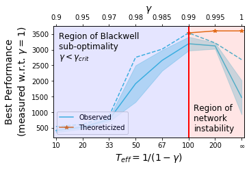
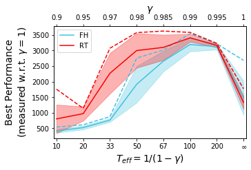
While Blackwell optimality (Blackwell, 1962) guarantees that there exists some such that solving for results in a policy optimal for the total reward; in practice, finding and solving for it, isn’t a simple task. As we show in Fig. 1, in practice, the performance of the agent can be characterized by two regions (the location of the border between both regions depends both on the environment and the algorithm):
-
1.
() The well known region of Blackwell sub-optimality . Here the planning horizon is insufficient. Long term rewards are discounted and thus have minuscule effect on the policy, resulting in myopic and sub-optimal behavior.
-
2.
() The region of network instability. While, in theory, one would expect behavior as presented in the ‘theoreticized’ line (performance improves with the increase of ), as conjectured above, the noise apparent in the learning process is too large and thus as continues to increase, the performance continues to degrade.
Previous work has highlighted the sub-optimality of the training regime and those attempting to overcome these issues are commonly referred to as Meta-RL algorithms. The term “Meta" refers to the algorithm adaptively changing the objective to improve performance. However, these methods commonly operate in an end-to-end scheme and are thus confined to optimizing the -discounted objective. For instance, Meta-gradients (Xu et al., 2018) optimize the policy on the inner-loss with respect to (w.r.t.) a learned whereas is optimized w.r.t. the outer-loss (the original objective). An additional work is LIRPG (Zheng et al., 2018), which learns an intrinsic reward function that, when combined with the extrinsic reward, guides the policy towards better performance in the -discounted task.
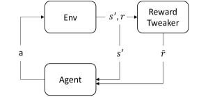
In this work, we take a different path. Our method, reward tweaking, learns a surrogate reward function . The surrogate reward is learned such that an agent maximizing in the -discounted setting, will be optimal w.r.t. the cumulative undiscounted reward . Fig. 2 illustrates our proposed framework. Thus reward tweaking enables the agent to find optimal policies even while optimizing over short horizons.
We formalize the task of learning as a classification problem and analyze it both theoretically and empirically. Specifically, we construct it in the form of finding the max-margin separator between trajectories, a supervised learning problem. We evaluate reward tweaking on both a tabular domain and a high dimensional continuous control task (Hopper-v2 (Todorov et al., 2012)). While our method does not mitigate the issues in the region of network instability, it improves the performance of the agent in the region of Blackwell sub-optimality, for all discount values (including at which is observed to perform best within the stable region).
2 Related Work
Reward Shaping: Reward shaping has been thoroughly researched from multiple directions. As the policy is a by-product of the reward, previous works defined classes of reward transformations that preserve the optimality of the policies. For instance, potential-based reward shaping that was proposed by Ng et al. (1999) and extended by Devlin and Kudenko (2012) that provided a dynamic method for learning such transformations online. While such methods aim to preserve the policy, others aim to shift it towards better exploration (Pathak et al., 2017) or attempt to improve the learning process (Chentanez et al., 2005; Zheng et al., 2018). However, while the general theme in reward shaping is that the underlying reward function is unknown, in reward tweaking we have access to the real returns and attempt to tweak the reward such that it enables overcoming the pitfalls of learning with small discount factors.
Direct Optimization: While practical RL methods typically solve the wrong task, i.e., the -discounted, there exist methods that can directly optimize the total reward. For instance, evolution strategies (Salimans et al., 2017) and augmented random search (Mania et al., 2018) perform a finite difference estimation of . This optimization scheme does not suffer from stability issues and can thus optimize the real objective directly. As these methods can be seen as a form of finite differences, they require complete evaluation of the newly suggested policies at each iteration, thus, in the general case, these procedures are sample inefficient.
Inverse RL and Trajectory Ranking: In Inverse RL (Ng et al., 2000; Abbeel and Ng, 2004; Syed and Schapire, 2008), the goal is to infer a reward function which explains the behavior of an expert demonstrator; or in other words, a reward function such that the optimal solution results in a similar performance to that of the expert. The goal in Trajectory Ranking (Wirth et al., 2017) is similar, however instead of expert demonstrations, we are provided with a ranking between trajectories. While previous work Brown et al. (2019) considered trajectory ranking to perform IRL; they focused on a set of trajectories, possibly strictly sub-optimal, which are provided apriori and a relative ranking between them. In this work, the trajectories are collected on-line using the behavior policy and the ranking is performed by evaluating the total reward provided by the environment.
3 Preliminaries
We consider a Markov Decision Process (Puterman, 1994, MDP) defined by the Tuple , where are the states, the actions, the reward function and is the transition kernel. The goal in RL is to learn a policy . While one may consider the set of stochastic policies, it is well known that there exists an optimal deterministic policy. In addition to the policy, we define the value function to be the expected reward-to-go of the policy and the quality function the utility of initially playing action and then acting based on policy afterwards.
In this work we focus on the episodic setting, where each episode is up to length (where is known and defined either by the user or the environment), and consider two objectives. (1) The discounted return where is the initial state distribution and the discount factor controls the effective planning horizon. (2) The total return
As we focus on the episodic setting, it is important to note that the optimal policy may not necessarily be stationary. This can easily be solved by appending the remaining horizon to the state (Dann and Brunskill, 2015).
When considering the discounted-episodic return, a well known result (Blackwell, 1962) is that there exists a critical discount factor , such that . In other words, there exists some high enough discount factor that induces optimality on the total-reward undiscounted objective ().
4 Maximizing the Total Reward when
Although the total reward is often the objective of interest, due to numerical optimization issues, empirical methods solve an alternative problem – the -discounted objective (Mnih et al., 2015; Hessel et al., 2017; Kapturowski et al., 2018; Badia et al., 2020). This re-definition of the task enables deep RL methods to solve complex high dimensional problems. However, in the general case, this may converge to a sub-optimal solution (Blackwell, 1962). We present such an example in Fig. 3, where taking the action left provides a reward and taking right . For rewards such as and the critical discount is . Here, results in the policy going to the right (maximizing the total reward in the process) and results in sub-optimal behavior, as the agent will prefer to go to the left.
We define a policy as the optimal policy for the -discounted task, and the value of this policy on the total undiscounted reward as .
The focus of this work is on learning with infeasible discount factors, which we define as the set of discount factors where is the minimal such that . Simply put, is the minimal discount factor where we can still solve the discounted task and remain optimal w.r.t. the total reward. This is motivated by the limitation imposed by current state-of-the-art algorithms (see Fig. 1), which typically do not work well for discount factors close to 1.


While previous methods attempted to overcome this issue through algorithmic improvements, e.g., attempting to increase the maximal supported by the algorithm (Kapturowski et al., 2018), we take a different approach. Our goal is to learn a surrogate reward function such that for any two trajectories , where , which induce returns then .
In layman’s terms, for a given discount we aim to find a new reward function . The agents objective will be to maximize the -discounted reward w.r.t. the new reward , however, we will continue to evaluate it on the original undiscounted reward . The goal of is to guide the agent towards better behavior on the original objective. Finally, it’s important to state that this problem is ill-defined. Similar to the results from Inverse RL, there exist an infinite number of reward functions which satisfy these conditions; our goal is to find one of them.
4.1 Existence of the Solution
We begin by proving existence of the solution. All proofs are provided in the appendix.
Theorem 1.
For any there exists a reward such that
Hence, by finding an optimal policy for the surrogate reward function in the -discounted case, we recover a policy that is optimal for the total reward.
Remark 1.
An important observation is that while the common theme in RL is to analyze MDPs with stationary reward functions; in our setting, as seen in Eq. 4, the surrogate reward function is not necessarily stationary. Hence, in the general case, must be time dependent.
Although there exists a reward for which (i.e., optimal w.r.t. the total reward), as the agent is not necessarily provided with this reward apriori, it raises a question as to can this reward be found. The following result tells us that indeed, in the finite horizon setting, such a reward can be found.
Theorem 2.
For any , there exists a mapping such that for any two trajectories and then .
While the above result motivates the online learning procedure, our focus in this work, it holds only for strictly bigger than . Thus, it many not be possible to reduce all RL tasks to a series of bandit problems (e.g., results in a myopic agent – a multi-stage bandit).
Proposition 1.
Theorem 2 does not hold for .
4.2 Robustness
In addition to analyzing the existence of the solution, we analyze the robustness gained by learning with an optimal surrogate reward function in the -discounted setting. Here, we assume that the reward is given and the agent solves the finite horizon -discounted reward , yet is evaluated on the undiscounted reward .
Kearns and Singh (1998) proposed the Simulation Lemma, which enables analysis of the value error when using an empirically estimated MDP. By extending their results to the finite horizon -discounted case, we show that in addition to improving rates of convergence, the optimal surrogate reward increases the robustness of the MDP to uncertainty in the transition matrix.
Proposition 2.
If enables recovering the optimal policy (e.g., Eq. 4), , where is the empirical probability transition estimates, and , then
As we are analyzing the finite-horizon objective, it is natural to consider a scenario where the uncertainty in the transitions is concentrated at the end of the trajectories. This setting is motivated by practical observations – the agent commonly starts in the same set of states, hence, most of the data it observes (higher confidence) is concentrated in those regions.
The following proposition presents how the bounds improve by a factor of when the uncertainty is concentrated near the end of the trajectories, as a factor of both the discount and the size of the uncertainty region defined by .
Proposition 3.
We assume the MDP can be factorized, such that all states that can be reached within steps are unreachable for , . We denote the reachable states by .
If and then
5 Learning the Surrogate Objective
Previously, we have discussed the existence and benefits provided by a reward function, which enables learning with smaller discount factors. In this section, we focus on how to learn the surrogate reward function .
With a slight abuse of notation, we define the set of previously seen trajectories and a sub-trajectory by . Our goal is to find a reward function that satisfies the ranking problem, for any and . That is, assuming , learning is done by solving:
| (1) |
Remark 2.
For a tabular state space, we may represent a trajectory by , and as a linear mapping. This is a logistic regression (Soudry et al., 2018), where the goal is to find the max-margin separator between trajectories
| (2) |
As we are concerned with maximizing the margin between all trajectories, the task becomes
| (3) |
As opposed to Brown et al. (2019, T-REX), we are not provided with apriori demonstrations and a ranking between them, instead, we follow an online scheme (Algorithm 1 and Fig. 2). As a part of the training phase, the trajectories observed by the policy are provided to the reward learner. The reward learner provides the most recent learned reward to the policy. As shown in Theorem 2, this ranking problem (Eq. 3) has a solution; thus (informally), assuming the policy has a non-zero support on each trajectory (i.e., each trajectory is observed infinitely often), Algorithm 1 will converge (in the limit) to the optimal policy.
6 Experiments
6.1 Tabular Reinforcement Learning
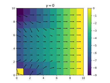
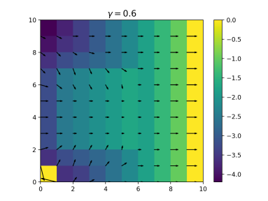
To understand how reward tweaking behaves, we analyze a grid-world, depicted in Fig. 4. Here, the agent starts at the bottom left corner and is required to navigate towards the goal (the wall on the right). Each step, the agent receives a reward of , whereas the goal, an absorbing state, provides . Clearly, the optimal solution is the stochastic shortest path. However, at the center resides a puddle where . The puddle serves as a distractor for the agent, creating a critical point at . While the optimal total reward is , an agent trained without reward tweaking for prefers to reside in the puddle and obtains a total reward of .
For analysis of plausible surrogate rewards, obtained by reward tweaking, we present the heatmap of a reward in each state, based on Eq. 4. As the reward is non-stationary, we plot the reward at the minimal reaching time, e.g., where is the Manhattan distance in the grid. The arrows represent the gradient of the surrogate reward , i.e., the policy of a myopic agent. Notice that when , the default reward signal is sufficient. However, in this domain, when the discount declines below the critical point, the 1-step surrogate reward (e.g., ) becomes informative enough for the myopic agent to find the optimal policy (the arrows represent the myopic policy). In other words, reward tweaking with small discount factors leads to denser rewards, resulting in an easier training phase for the policy.

6.2 Deep Reinforcement Learning
In addition to analyzing reward tweaking in the tabular domain, we evaluate it on a complex task, using approximation schemes (deep neural networks). We focus on Hopper (Todorov et al., 2012), a finite-horizon () robotic control task where the agent controls the torque applied to each motor. We build upon the TD3 algorithm (Fujimoto et al., 2018), a deterministic off-policy policy-gradient method (Silver et al., 2014; Lillicrap et al., 2015), that combines two major components – an actor and a critic. The actor maps from state to action , i.e., the policy; and the critic is trained to predict the expected return. Our implementation is based on the original code provided by Fujimoto et al. (2018), including their original hyper-parameters. For each value of , we compare 5 randomly sampled seeds, showing the mean and confidence interval of the mean. This results in a total of 40 seeds.
6.2.1 Experimental Details
We compare reward tweaking with the baseline TD3 model, adapted to the finite horizon setting. We provide additional experiments details in the supplementary material, in addition to numerical results. Graphical results are provided in Fig. 5.
As we are interested in a finite-horizon task, the reward tweaking experiments are performed on a non-stationary version of TD3, i.e., we concatenate the normalized remaining time to the state. In our experiments111Code accompanying this paper is provided in bit.ly/2O1klVu, and are learned in parallel (Fig. 2). In order to learn , we sample trajectories up to length of steps. This is a computational consideration – a larger will lead to better performance, but will result in a longer run-time. Experimentally, we found to suffice. As is trained on , the model is required to extrapolate for (a similar trade-off exists in standard back-propagation through time (Sutskever, 2013)).
6.2.2 Results
We present the results in Fig. 5 and the numerical values in the supplementary material. For each discount and model, we run a simulation using 5 random seeds. For each seed, at the end of training, we re-evaluate (over episodes) the policy that is believed to be best. The results we report are the average, STD and the max of these values (over the simulations performed).
Baseline analysis: The baseline behaves best at . This leads to two important observations. (1) Although the model is fit for a finite-horizon task, and the horizon is indeed finite, it fails when the effective planning horizon increases above (). This suggests that practical algorithms have a maximal feasible discount value, such that for larger values they suffer from performance degradation. (2) As decreases, the agent becomes myopic leading to sub-optimal behavior.
These results motivate the use of reward tweaking. While reward tweaking is incapable of overcoming the first problem, it is designed to mitigate the second – the failure which occurs due to not satisfying the Blackwell optimality criteria (Blackwell, 1962).
Reward Tweaking: (1) As hypothesised, reward tweaking improves the performance across all feasible discount values, i.e., values where TD3 is capable of learning (). (2) Learning the reward becomes harder as decreases, hence the variance across seeds grows as the planning horizon decreases. Finally, (3) focusing on the maximal performance across seeds, we see that while this is a hard task, reward tweaking improves the performance in terms of average and maximal score – and even improves the average performance at (the maximal feasible discount for the TD3 baseline on this task) from to ( performance improvement).
7 Conclusions
In this work we tackled the problem of learning with Blackwell sub-optimality; the algorithm aims to maximize the total reward, yet is limited to learning with sub-optimal discount factors. We proposed reward tweaking, a method for learning a reward function which induces better behavior on the original task. Our proposed method enables the learning algorithm to find optimal policies, by learning a new reward function . We showed, in the tabular case, that there indeed exists such a reward function. In addition, we proposed an objective to solving this task, which is equivalent to finding the max-margin separator between trajectories.
We evaluated reward tweaking in a tabular setting, where the reward is ensured to be recoverable, and in a high dimensional continuous control task. In the tabular case, visualization enables us to analyze the structure of the learned rewards, suggesting that reward tweaking learns dense reward signals – these are easier for the learning algorithm to learn from. In the Hopper domain, our results show that reward tweaking is capable of outperforming the baseline across most planning horizons. Finally, we observe that while learning a good reward function is hard for short planning horizons, in some seeds, reward tweaking is capable of finding good reward functions. This suggests that further improvement in stability and parallelism of the reward learning procedure may further benefit this method.
Although in terms of performance reward tweaking has many benefits, this method has a computational cost. Even though learning the surrogate reward does not require additional interactions with the environment (sample complexity), it does require a significant increase in computation power (wallclock time). As we sample partial trajectories and compute the loss over the entirety of them, this requires many more computations when compared to the standard TD3 scheme. Thus, it is beneficial to use reward tweaking when the performance degradation, due to the use of infeasible discount factors, is large, or when sample efficiency is of utmost importance.
We focused on scenarios where the algorithm is incapable of solving for the correct . Future work can extend reward tweaking to additional capabilities. For instance, to stabilize learning, many works clip the reward to (Mnih et al., 2015). However, these changes, like the discount factor, change the underlying task the agent is solving. Reward tweaking can be used to find rewards which satisfy these constraints, yet still induce optimal behavior on the total original reward.
Finally, while reward tweaking has a computational overhead, it comes with significant benefits. Once an optimal surrogate reward has been found, it can be re-used in future training procedures. As it enables the agent to solve the task using smaller discount factors, given a learned , the policy training procedure is potentially faster.
8 Broader Impact
Reward tweaking tackles a fundamental problem in applied reinforcement learning. As reinforcement learning algorithms commonly optimize the discounted infinite horizon objective, they underperform on the required metric – the undiscounted total reward.
Reward tweaking bridges the gap between the objective we want to solve and that which our algorithms are capable of solving. As such, reward tweaking has the potential to impact reinforcement learning on a broad scale across almost all application levels. These applications range from physical applications (e.g., robotics, autonomous vehicles, warehouse automation, and more) and digital applications (e.g., marketing, recommendation systems, and more).
References
- Abbeel and Ng [2004] Pieter Abbeel and Andrew Y Ng. Apprenticeship learning via inverse reinforcement learning. In Proceedings of the twenty-first international conference on Machine learning, page 1. ACM, 2004.
- Amit et al. [2020] Ron Amit, Kamil Ciosek, and Ron Meir. Discount factor as a regularizer in reinforcement learning. In International Conference on Machine Learning, 2020.
- Badia et al. [2020] Adrià Puigdomènech Badia, Bilal Piot, Steven Kapturowski, Pablo Sprechmann, Alex Vitvitskyi, Daniel Guo, and Charles Blundell. Agent57: Outperforming the atari human benchmark. arXiv preprint arXiv:2003.13350, 2020.
- Blackwell [1962] David Blackwell. Discrete dynamic programming. The Annals of Mathematical Statistics, pages 719–726, 1962.
- Brown et al. [2019] Daniel Brown, Wonjoon Goo, Prabhat Nagarajan, and Scott Niekum. Extrapolating beyond suboptimal demonstrations via inverse reinforcement learning from observations. In International Conference on Machine Learning, pages 783–792, 2019.
- Chentanez et al. [2005] Nuttapong Chentanez, Andrew G Barto, and Satinder P Singh. Intrinsically motivated reinforcement learning. In Advances in neural information processing systems, pages 1281–1288, 2005.
- Dann and Brunskill [2015] Christoph Dann and Emma Brunskill. Sample complexity of episodic fixed-horizon reinforcement learning. In Advances in Neural Information Processing Systems, pages 2818–2826, 2015.
- Devlin and Kudenko [2012] Sam Michael Devlin and Daniel Kudenko. Dynamic potential-based reward shaping. In Proceedings of the 11th International Conference on Autonomous Agents and Multiagent Systems, pages 433–440. IFAAMAS, 2012.
- Efroni et al. [2018] Yonathan Efroni, Gal Dalal, Bruno Scherrer, and Shie Mannor. Beyond the one-step greedy approach in reinforcement learning. In International Conference on Machine Learning, pages 1386–1395, 2018.
- Fujimoto et al. [2018] Scott Fujimoto, Herke Hoof, and David Meger. Addressing function approximation error in actor-critic methods. In International Conference on Machine Learning, pages 1582–1591, 2018.
- Haarnoja et al. [2018] Tuomas Haarnoja, Aurick Zhou, Pieter Abbeel, and Sergey Levine. Soft actor-critic: Off-policy maximum entropy deep reinforcement learning with a stochastic actor. arXiv preprint arXiv:1801.01290, 2018.
- Hessel et al. [2017] Matteo Hessel, Joseph Modayil, Hado Van Hasselt, Tom Schaul, Georg Ostrovski, Will Dabney, Dan Horgan, Bilal Piot, Mohammad Azar, and David Silver. Rainbow: Combining improvements in deep reinforcement learning. arXiv preprint arXiv:1710.02298, 2017.
- Kapturowski et al. [2018] Steven Kapturowski, Georg Ostrovski, John Quan, Remi Munos, and Will Dabney. Recurrent experience replay in distributed reinforcement learning. 2018.
- Kearns and Singh [1998] Michael J Kearns and Satinder P Singh. Near-optimal reinforcement learning in polynominal time. In Proceedings of the Fifteenth International Conference on Machine Learning, pages 260–268. Morgan Kaufmann Publishers Inc., 1998.
- Lillicrap et al. [2015] Timothy P Lillicrap, Jonathan J Hunt, Alexander Pritzel, Nicolas Heess, Tom Erez, Yuval Tassa, David Silver, and Daan Wierstra. Continuous control with deep reinforcement learning. arXiv preprint arXiv:1509.02971, 2015.
- Mania et al. [2018] Horia Mania, Aurelia Guy, and Benjamin Recht. Simple random search provides a competitive approach to reinforcement learning. arXiv preprint arXiv:1803.07055, 2018.
- Mnih et al. [2015] Volodymyr Mnih, Koray Kavukcuoglu, David Silver, Andrei A Rusu, Joel Veness, Marc G Bellemare, Alex Graves, Martin Riedmiller, Andreas K Fidjeland, Georg Ostrovski, et al. Human-level control through deep reinforcement learning. Nature, 518(7540):529, 2015.
- Ng et al. [1999] Andrew Y Ng, Daishi Harada, and Stuart Russell. Policy invariance under reward transformations: Theory and application to reward shaping. In ICML, volume 99, pages 278–287, 1999.
- Ng et al. [2000] Andrew Y Ng, Stuart J Russell, et al. Algorithms for inverse reinforcement learning. In Icml, volume 1, page 2, 2000.
- Pathak et al. [2017] Deepak Pathak, Pulkit Agrawal, Alexei A Efros, and Trevor Darrell. Curiosity-driven exploration by self-supervised prediction. In International Conference on Machine Learning, pages 2778–2787, 2017.
- Puterman [1994] Martin L Puterman. Markov decision processes: discrete stochastic dynamic programming. John Wiley & Sons, 1994.
- Salimans et al. [2017] Tim Salimans, Jonathan Ho, Xi Chen, Szymon Sidor, and Ilya Sutskever. Evolution strategies as a scalable alternative to reinforcement learning. arXiv preprint arXiv:1703.03864, 2017.
- Schulman et al. [2017] John Schulman, Filip Wolski, Prafulla Dhariwal, Alec Radford, and Oleg Klimov. Proximal policy optimization algorithms. arXiv preprint arXiv:1707.06347, 2017.
- Silver et al. [2014] David Silver, Guy Lever, Nicolas Heess, Thomas Degris, Daan Wierstra, and Martin Riedmiller. Deterministic policy gradient algorithms. In International Conference on Machine Learning, pages 387–395, 2014.
- Soudry et al. [2018] Daniel Soudry, Elad Hoffer, Mor Shpigel Nacson, Suriya Gunasekar, and Nathan Srebro. The implicit bias of gradient descent on separable data. The Journal of Machine Learning Research, 19(1):2822–2878, 2018.
- Sutskever [2013] Ilya Sutskever. Training recurrent neural networks. University of Toronto Toronto, Ontario, Canada, 2013.
- Syed and Schapire [2008] Umar Syed and Robert E Schapire. A game-theoretic approach to apprenticeship learning. In Advances in neural information processing systems, pages 1449–1456, 2008.
- Tessler et al. [2017] Chen Tessler, Shahar Givony, Tom Zahavy, Daniel J Mankowitz, and Shie Mannor. A deep hierarchical approach to lifelong learning in minecraft. In AAAI, volume 3, page 6, 2017.
- Todorov et al. [2012] Emanuel Todorov, Tom Erez, and Yuval Tassa. Mujoco: A physics engine for model-based control. In Intelligent Robots and Systems (IROS), 2012 IEEE/RSJ International Conference on, pages 5026–5033. IEEE, 2012.
- Wirth et al. [2017] Christian Wirth, Riad Akrour, Gerhard Neumann, and Johannes Fürnkranz. A survey of preference-based reinforcement learning methods. The Journal of Machine Learning Research, 18(1):4945–4990, 2017.
- Xu et al. [2018] Zhongwen Xu, Hado P van Hasselt, and David Silver. Meta-gradient reinforcement learning. In Advances in neural information processing systems, pages 2396–2407, 2018.
- Zheng et al. [2018] Zeyu Zheng, Junhyuk Oh, and Satinder Singh. On learning intrinsic rewards for policy gradient methods. In Advances in Neural Information Processing Systems, pages 4644–4654, 2018.
Appendix A Proofs
Theorem 3.
For any there exists such that
Where is the original reward and is the horizon.
Proof.
We define the optimal value function for the finite-horizon total reward by , the optimal policy and the value of the surrogate objective with discount by . Thus, extending the result shown in Efroni et al. [2018, -PI], we may define the surrogate reward as
| (4) |
Applying the Bellman operator, we get
As we only added a fixed term to the reward, trivially, under the optimal Bellman operator we have that . Also, this has a single fixed-point :
| (5) | ||||
the above holds for any . ∎
Theorem 4.
For any , there exists a mapping such that for any two trajectories and then .
Proof.
While the problem is ill-defined, e.g., there exists many reward signals which satisfy this condition, finding one such reward is sufficient for existence.
Consider the reward . For any two trajectories the following holds:
| (6) |
hence, if then . ∎
Proposition 4.
Theorem 2 does not hold for .
Proof.
Consider 3 trajectories:
where the rewards are
thus the following ordering holds .
However, by setting the utility of each trajectory in the -discounted setting is defined as
thus, and the ordering can not be maintained. ∎
Lemma 1.
For any MDP , the surrogate reward for the -discounted problem is not unique.
Proof.
This can be shown trivially, by observing that any multiplication of the rewards by a positive (non-zero) scalar, is identical. Meaning that, :
∎
Proposition 5.
If enables recovering the optimal policy, e.g., Eq. 4, and , where is the empirical probability transition estimates, then
where .
Proof.
The proof follows that of the Simulation Lemma, with a slight adaptation for the finite horizon discounted scenario with zero reward error.
where . Moreover, in order to recover the bounds for the original problem, plugging in Theorem 1 we retrieve the original value and thus ; in which the robustness is improved by a factor of . ∎
As we are analyzing the finite-horizon objective, it is natural to consider a scenario where the uncertainty in the transitions is concentrated at the end of the trajectories. This setting is motivated by practical observations – the agent commonly starts in the same set of states, hence, most of the data it observes is concentrated in those regions leading to larger errors at advanced stages.
The following proposition presents how the bounds improve when the uncertainty is concentrated near the end of the trajectories, as a factor of both the discount and the size of the uncertainty region defined by .
Proposition 6.
We assume the MDP can be factorized, such that all states that can be reached within steps are unreachable for , . We denote the reachable states by .
If and then
Proof.
Notice that this formulation defines a factorized MDP, in which we can analyze each portion independently.
The sub-optimality of for can be bounded similarly to Proposition 2
where the horizon is due to the factorization of the MDP.
For , clearly as the estimation error is for states near the initial position, then the overall error in these states is bounded by where is due to the steps it takes to reach the uncertainty region. ∎
Appendix B Extended Results
B.1 Experimental Details
We compare reward tweaking with the baseline TD3 model, adapted to the finite horizon setting. The results are presented graphically in Fig. 5 and numerically in the supplementary material. Our implementations are based on the original code by Fujimoto et al. [2018]. In their work, as they considered stationary models, they converted the task into an infinite horizon setting, by considering “termination signals due to timeout" as non-terminal. However, they still evaluate the policies on the total reward achieved over steps.
Although this works well in the MuJoCo control suite, it is not clear if this should work in the general case, and whether or not the algorithm designer has access to this knowledge (that termination occurred due to timeout). Hence, we opt for a finite-horizon non-stationary actor and critic scheme. To achieve this, we concatenate the normalized remaining time to the state.
As we are interested in a finite-horizon task, the reward tweaking experiments are performed on this non-stationary version of TD3. In our experiments, and are learned in parallel (Fig. 2). The reward tweaker , is represented using 4 fully-connected layers () with ReLU activations. Training is performed on trajectories, which are sampled from the replay buffer, every time-steps. Each time, the loss is computed using trajectories, each up to a length of steps. Due to the structure of the environment, timeout can occur at any state. Hence, given a sampled sub-trajectory, we update the normalized remaining time of the sampled states, based on the length of the sub-trajectory, i.e., as if timeout occurred in the last sampled state. This enables to train using partial trajectories, while the model is required to extrapolate the rest. Our computing infrastructure consists of two machines with two GTX 1080 GPUs, each.
| Baseline | Avg. | ||||
|---|---|---|---|---|---|
| Max | |||||
| Reward Tweaking | Avg. | ||||
| Max |
| Baseline | Avg. | ||||
|---|---|---|---|---|---|
| Max | |||||
| Reward Tweaking | Avg. | ||||
| Max |