Pulsar timing array signals induced by black hole binaries in relativistic eccentric orbits

Abstract

Individual supermassive black hole binaries in non-circular orbits are possible nanohertz gravitational wave sources for the rapidly maturing Pulsar Timing Array experiments. We develop an accurate and efficient approach to compute Pulsar Timing Array signals due to gravitational waves from inspiraling supermassive black hole binaries in relativistic eccentric orbits. Our approach employs a Keplerian-type parametric solution to model third post-Newtonian accurate precessing eccentric orbits while a novel semi-analytic prescription is provided to model the effects of quadrupolar order gravitational wave emission. These inputs lead to a semi-analytic prescription to model such signals, induced by non-spinning black hole binaries inspiralling along arbitrary eccentricity orbits. Additionally, we provide a fully analytic prescription to model Pulsar Timing Array signals from black hole binaries inspiraling along moderately eccentric orbits, influenced by Boetzel et al. [Phys. Rev. D 96,044011(2017)]. These approaches are being incorporated into Enterprise and TEMPO2 for searching the presence of such binaries in Pulsar Timing Array datasets.

I Introduction

Pulsar Timing Array (PTA) experiments are expected to inaugurate the field of nanohertz gravitational wave (GW) astronomy during the next decade (Kelley et al., 2017). This will augment the ground-based GW astronomy, established by the LIGO Scientific Collaboration and the Virgo collaboration during the present decade, operating mainly in the hectohertz to kilohertz frequency regime (The LIGO Scientific Collaboration and the Virgo Collaboration, 2018). A PTA experiment monitors an ensemble of millisecond pulsars (MSPs) to search for correlated deviations to their pulse times of arrival (TOAs) to infer the presence of GWs (Foster and Backer, 1990). These efforts are sensitive to long-wavelength ($\sim$1 nHz – 100 nHz) GWs, where the lower and upper limits of the frequency range are respectively set by the total span and cadence of the PTA observations (Lommen, 2015). Therefore, PTAs are expected to detect GWs from supermassive black hole (SMBH) binaries with milliparsec orbital separations (Detweiler, 1979). At present, there exist three matured PTA efforts, namely the Parkes Pulsar Timing Array (PPTA) (Hobbs, 2013), the European Pulsar Timing Array (EPTA) (Kramer and Champion, 2013), and the North American Nanohertz Observatory for Gravitational Waves (NANOGrav) (McLaughlin, 2013; Brazier et al., 2019). Additionally, there are emerging PTA efforts from India, China, and South Africa (Joshi et al., 2018; Bailes et al., 2018; Lee, 2016). The International Pulsar Timing Array (IPTA) consortium combines data and resources to achieve more quickly the first detection of nanohertz GWs (Hobbs et al., 2010; Verbiest et al., 2016; Perera et al., 2019).

There are a number of promising astrophysical and cosmological GW sources in the nanohertz frequency window (Hobbs and Dai, 2017; Burke-Spolaor et al., 2019). We expect the first detected signal to be the ensemble of GWs from many SMBH binaries, producing a stochastic GW background (SGWB). This should be followed by the detection of bright individual SMBH binaries that resound above this background Rosado et al. (2015); Kelley et al. (2018). Stringent observational constraints are being placed on both types of PTA sources due to the absence of any firm detections in the PTA datasets (Arzoumanian et al., 2018; Aggarwal et al., 2019; Babak et al., 2015; Lentati et al., 2015; Feng et al., 2019; Porayko et al., 2018). In the case of SMBH binaries in circular orbits, the present sky-averaged upper limit on GW strain is below $7.3\times 10^{-15}$ at $8$ nHz (Aggarwal et al., 2019).

Such constraints on SMBH binaries can be invoked to restrict their astrophysical formation and evolution scenarios (Middleton et al., 2018; Chen et al., 2019, 2017; Taylor et al., 2019, 2017). It will be desirable to extend the above bounds to eccentric binaries since SMBH binaries emitting nanohertz GWs can have non-negligible orbital eccentricities (Burke-Spolaor et al., 2019). It was noted that SMBH binaries originating from gas-rich galaxy mergers may have non-negligible eccentricities even during their late inspiral phase (Armitage and Natarajan, 2005; Cuadra et al., 2009). Additionally, realistic N-body simulations of massive galaxy mergers result in SMBH binaries in eccentric orbits due to stellar interactions (Berentzen et al., 2009; Khan et al., 2012, 2013; Roedig and Sesana, 2012). Therefore, it will be interesting to probe the presence of such binaries in the existing PTA datasets. This demands general relativistic constructs that can be implemented in the popular pulsar timing software packages like TEMPO2 and Enterprise (Edwards et al., 2006; Hobbs et al., 2006; Ellis et al., 2017).

In the present paper, we develop an accurate and efficient prescription to obtain PTA signals induced by isolated SMBH binaries inspiraling along general relativistic eccentric orbits. Our approach employs the post-Newtonian (PN) approximation which allows us to model black holes (BHs) as point particles (Blanchet, 2014). Recall that PN approximation provides general relativistic corrections to Newtonian dynamics in powers of $({v}/{c})^{2}\sim{GM}/{c^{2}r}$, where $v$, $M$, and $r$ are respectively the relative velocity, total mass, and relative separation of a BH binary. We let BH binaries move in 3PN-accurate precessing eccentric orbits with the help of generalized quasi-Keplerian parametrization (Memmesheimer et al., 2004), where the 3PN-accurate description incorporates $(\frac{v}{c})^{6}$-order general relativistic corrections to Newtonian motion. Additionally, we incorporate the effects of GW emission at the dominant quadrupolar order with the help of a GW phasing formalism, detailed in Damour2006,KonigsdorfferGopakumar2006,Refs. Ref. Damour et al. (2004); Königsdörffer and Gopakumar (2006), while adapting recent results from Moore2018,Refs. Ref. Moore et al. (2018). This allows us to model PTA signals due to non-spinning SMBH binaries inspiraling along 3PN-accurate eccentric orbits in a semi-analytic manner. The numerical treatments are required only to solve the PN-accurate Kepler equation and to integrate the resulting fractional pulsar frequency shift induced by passing GWs. These considerations ensure that the prescription is general relativistically accurate and computationally efficient. It turns out that the PN description is quite appropriate to model such PTA signals as the SMBH binaries are expected to merge at orbital frequencies outside the PTA frequency window (Burke-Spolaor et al., 2019). Additionally, we provide a fully-analytic prescription to compute PTA signals induced by isolated SMBH binaries inspiraling along moderately eccentric orbits. This result heavily depends on a fully analytic approach to compute temporally evolving GW polarization states for compact binaries moving in PN-accurate moderately eccentric orbits (Boetzel et al., 2017). We note in passing that the present effort extends and improves efforts to compute PTA signals due to GWs from compact binaries inspiraling along Newtonian accurate eccentric orbits (Jenet et al., 2004; Taylor et al., 2016).

In what follows, we list below the salient features of the present paper.

• A brief description of our approach for computing quadrupolar-order PTA signals due to inspiral GWs from non-spinning massive BH binaries in PN-accurate precessing eccentric orbits while employing the PN-accurate Keplerian-type parametric solution and the GW phasing approach of Ref. Damour et al. (2004) is presented in Sec. II.1 and II.2.

• An accurate and computationally efficient way to incorporate the effects of GW emission on the parametrized conservative PN-accurate orbital dynamics and its salient features are presented in Sec. II.3. This subsection explains why we require a one-time numerical solution of a differential equation to incorporate the effects of quadrupolar GW emission in our approach. Plots displaying PTA signals that arise from our semi-analytical approach and their various facets are provided in Sec. II.4. The computational costs associated with our modeling of the PTA signals, induced by GWs from massive BH binaries in PN-accurate arbitrary eccentricity orbits are provided in Sec. II.5.

• A fully analytic way of computing PTA signals for moderate eccentricities ($e\lesssim 0.3$) is presented in Sec. III where we employed crucial inputs from Ref. Boetzel et al. (2017). This approach provides a powerful check on our detailed semi-analytic prescription and this is demonstrated by comparing PTA signals computed using our semi-analytic and fully analytic methods in the low-eccentricity regime.

In brief, we developed an accurate and efficient prescription to compute PTA signals induced by isolated SMBH binaries inspiraling along general relativistic eccentric orbits, employing for the first time an accurate semi-analytic solution to describe PN-accurate orbital evolution of BH binaries. An implementation of the PTA signals derived in this work is available at https://github.com/abhisrkckl/GWecc.

II PTA signals from BH binaries in quasi-Keplerian eccentric orbits

We begin by deriving expressions for the dominant quadrupolar order $+/\times$ residuals in Sec. II.1. How we describe temporal evolution of various dynamical variables that appear in these expressions is described in Sec. II.2 and Sec. II.3, which is followed by a pictorial exploration of our main results in Sec. II.4 and an exploration of the associated computational costs in Sec. II.5. The present paper explores the effects of far-zone GWs on the pulsar TOAs, and this is realistic as our GW sources are extra-galactic while the pulsars exist within our Galaxy.

II.1 Timing residual expressions at the dominant quadrupolar order

When a GW signal passes across the line of sight between a pulsar and the observer along a direction $\hat{n}$, it perturbs the underlying space-time metric. This induces temporally evolving changes in the measured pulsar rotational frequency $\nu$ (Book and Flanagan, 2011)

$$\frac{\Delta\nu(t_{E})}{\nu}\equiv z_{\text{GW}}(t_{E})=h(t_{E})-h(t_{P})\,,$$ (1)

where $h$ stands for the dimensionless GW strain, $t_{E}$ and $t_{P}$ denote respectively the instances when a GW passes the solar system barycenter (SSB) and the pulsar, and the rotational frequency $\nu$ is measured in the SSB frame. These two time instances differ by the usual geometric delay such that

$$t_{P} =t_{E}-\frac{D_{P}}{c}\left(1+\hat{n}\cdot\hat{p}\right)$$

$$=t_{E}-\frac{D_{P}}{c}(1-\cos\mu)\,,$$ (2)

where $D_{P}$ is the distance to the pulsar while $\hat{p}$ specifies its direction with respect to the SSB, and $\mu$ provides the angle between $\hat{n}$ and $\hat{p}$. Influenced by Wahlquist1987,Refs. Ref. Wahlquist (1987), the GW strain $h$ can be written in terms of the two GW polarization states $h_{+,\times}$ as

$$h(t)=\begin{bmatrix}F_{+}&F_{\times}\end{bmatrix}\begin{bmatrix}\cos 2\psi&-\sin 2\psi\\ \sin 2\psi&\cos 2\psi\end{bmatrix}\begin{bmatrix}h_{+}(t)\\ h_{\times}(t)\end{bmatrix}\,,$$ (3)

where $F_{+,\times}$ are the antenna pattern functions that depend on the sky locations of the pulsar and the GW source, and $\psi$ is the polarization angle of the GW. The explicit expressions for $F_{+,\times}$ involve angles that specify the directions $\hat{n}$ and $\hat{p}$ (namely, the right ascension (RA) and declination (DEC) of the GW source and the pulsar), and are available in Lee2011,Refs. Ref. Lee et al. (2011).

The temporally evolving GW-induced redshift causes differences between the expected and the observed TOAs of pulses. This is given by

$$R(t_{E}) =\int_{0}^{t_{E}}z_{\text{GW}}(t^{\prime})\,dt^{\prime}=s(t_{E})-s(t_{P})\,,$$ (4)

where $s(t)$ is given by

$$s(t) =\int_{0}^{t}h(t^{\prime})dt^{\prime}=F_{+}s_{+}(t)+F_{\times}s_{\times}(t)\,,$$ (5)

and we have defined

$$s_{+,\times}(t)=\int_{0}^{t}h_{+,\times}(t^{\prime})\,dt^{\prime}\,.$$ (6)

This quantity $R(t_{E})$ is usually referred to as the GW-induced (pre-fit) pulsar timing residual or the PTA signal, and is essentially prescribed by the values of $s_{+,\times}$ at the SSB and the pulsar positions. It is customary to refer to $s(t_{E})$ and $s(t_{P})$ as the Earth and pulsar terms, and $s_{+,\times}$ as the plus/cross residuals, respectively.

The leading quadrupolar order $h_{+,\times}$ expressions for a non-spinning eccentric binary, available in Boetzel2017,Refs. Ref. Boetzel et al. (2017), read

$$h_{+}^{Q} =\frac{GM\eta}{D_{L}\,c^{2}}x\frac{1}{(1-\chi)^{2}}\left(-2\left(c_{i}^{2}+1\right)\sqrt{1-e_{t}^{2}}\xi\sin(2\phi)+\left(c_{i}^{2}+1\right)\left(2e_{t}^{2}-\chi^{2}+\chi-2\right)\cos(2\phi)+s_{i}^{2}(1-\chi)\chi\right)\,,$$ (7a)

$$h_{\times}^{Q} =\frac{GM\eta}{D_{L}\,c^{2}}x\frac{1}{(1-\chi)^{2}}2c_{i}\left(2\sqrt{1-e_{t}^{2}}\,\xi\cos(2\phi)+\left(2e_{t}^{2}-\chi^{2}+\chi-2\right)\sin(2\phi)\right)\,,$$ (7b)

where $\phi$ denotes the angular coordinate in the orbital plane, called the orbital phase (see Eqs. 9b and 14 below for the definition of $\phi$ for Newtonian and PN-accurate orbits) while the superscript $Q$ indicates the quadrupolar order contributions to $h_{+,\times}$. The total mass, symmetric mass ratio and luminosity distance to the binary are represented by $M=m_{1}+m_{2}$, $\eta=\frac{m_{1}m_{2}}{M^{2}}$, and $D_{L}$ respectively. Further, we use shorthand notations to denote trigonometric functions of the orbital inclination $i$, namely $c_{i}=\cos i$ and $s_{i}=\sin i$, while $\chi=e_{t}\cos u$ and $\xi=e_{t}\sin u$, where $u$ is the eccentric anomaly. The orbital eccentricity is specified by $e_{t}$ and it is associated with the PN-accurate Kepler equation (Memmesheimer et al., 2004). The dimensionless PN parameter $x=(GMn/c^{3})^{2/3}$ employs the mean motion $n$ associated with the Kepler equation, which is related to the orbital period $P_{b}$ by $n=2\pi/P_{b}$. In addition, the polarization angle $\psi$ present in Eq. (3) provides a measure of the longitude of the ascending node in the case of non-spinning binaries.

To obtain Eqs. (7), we begin from the quadrupolar order $h_{+,\times}$ expressions that are valid for compact binaries in non-circular orbits Damour et al. (2004)

$$h_{+}^{Q}(r,\phi,\dot{r},\dot{\phi}) =-\frac{GM\eta}{D_{L}c^{4}}\left[\left(1+c_{i}^{2}\right)\left[\left(\frac{GM}{r}+r^{2}\dot{\phi}^{2}-\dot{r}^{2}\right)\cos 2\phi+2r\dot{r}\dot{\phi}\sin 2\phi\right]+s_{i}^{2}\left(\frac{GM}{r}-r^{2}\dot{\phi}^{2}-\dot{r}^{2}\right)\right]\,,$$ (8a)

$$h_{\times}^{Q}(r,\phi,\dot{r},\dot{\phi}) =-\frac{GM\eta}{D_{L}c^{4}}2c_{i}\left[\left(\frac{GM}{r}+r^{2}\dot{\phi}^{2}-\dot{r}^{2}\right)\sin 2\phi-2r\dot{r}\dot{\phi}\cos 2\phi\right]\,,$$ (8b)

where $r$ and $\phi$ provide the radial and angular coordinates that specify the position of the reduced mass $m_{1}m_{2}/M$ around the total mass $M$ in the center of mass frame of the binary, while $\dot{r}=dr/dt$ and $\dot{\phi}=d\phi/dt$. We employ the Keplerian parametric solution for eccentric orbits to provide parametric expressions for these dynamical variables. The classical Keplerian parametric solution, neatly summarized in DamourDeruelle1985,Refs. Ref. Damour and Deruelle (1985), provides the following parametric expressions for $r$ and $\phi$:

$$r =a\,\left(1-e\,\cos u\right)\,,$$ (9a)

$$\phi-\phi_{0} =f\,,$$ (9b)

where $a$ and $e$ specify respectively the orbital semi-major axis and the Newtonian orbital eccentricity such that $0\leq e<1$, while $\phi_{0}$ is some initial orbital phase. The true anomaly $f$ is related to the eccentric anomaly $u$ by the relation

$$f=2\arctan\left[\left(\frac{1+e}{1-e}\right)^{1/2}\tan\frac{u}{2}\right]\,.$$ (10)

This approach provides temporal evolution for $r$ and $\phi$ in a semi-analytic manner as $u$ is related to the coordinate time $t$ by the transcendental Kepler equation (Damour and Deruelle, 1985)

$$l\equiv n(t-t_{0})=u-e\sin u\,,$$ (11)

where $l$ is called the mean anomaly and $t_{0}$ denotes the epoch of periapsis passage.

With the help of the such a parametric solution, it is fairly easy to obtain expressions for $r$, $\dot{r}$, and $\dot{\phi}$ in terms of $u$, $e$ and $x$. This essentially leads to Eqs. (7) from Eqs. (8) for $h_{+,\times}^{Q}$. Note that we need an accurate and efficient method to tackle the above transcendental Eq. (11) to obtain the actual temporal evolution for the two polarization states. We note in passing that Eqs. (7) and (8) are also invoked to obtain inspiral templates for stellar mass compact binaries in eccentric binaries Tanay et al. (2016); Tiwari et al. (2019).

In the next subsection, we summarize our approach to provide fully 3PN-accurate temporal evolution for our $h_{+,\times}^{Q}$ expressions.

II.2 Accurate description for the evolution of non-spinning BH binaries inspiraling along precessing eccentric orbits

We begin by outlining our approach to describe the orbital evolution of non-spinning BH binaries inspiraling along 3PN-accurate quasi-Keplerian eccentric orbits. This prescription is crucial to specify how the angular variables ($\phi,u$) and the orbital elements ($n,e_{t}$) vary in time while computing $R(t)$ as evident from Eqs. (7). First, we adapt the GW phasing formalism, detailed in Damour2006,KonigsdorfferGopakumar2006,Refs. Ref. Damour et al. (2004); Königsdörffer and Gopakumar (2006), for computing temporally evolving $h_{+,\times}(t)$. This approach involves splitting the orbital dynamics of compact binaries into certain conservative and reactive parts. In the PN terminology, the conservative dynamics usually provides PN corrections that are even powers of $(v/c)$, while reactive dynamics involves odd powers of $(v/c)$ beginning with ${\cal O}((v/c)^{5})$ contributions. Such a split is justified as the reactive effects due to GW emission first enter the orbital dynamics only at the $(v/c)^{5}$ (2.5PN) order and act in timescales much longer than the orbital period when the binary is not close to its merger. This split also allows us to employ PN-accurate Keplerian-type parametric solution for describing the 3PN-accurate conservative orbital dynamics, detailed in Memmesheimer2004,Refs. Ref. Memmesheimer et al. (2004). Extending Eq. (9b) to 3PN order, we write the 3PN-accurate orbital phase as

$$\phi-\phi_{0} =(1+k)\,l+W(u(l),n,e_{t})\,,$$ (12)

where the angular variable $W(u)$ is $2\pi$ periodic in $u$, and $k$ represents the advance of periapsis per orbit Damour et al. (2004); Königsdörffer and Gopakumar (2006). We do not display here the explicit 3PN-accurate expressions for $k$ and $W(u)$ in terms of $n$, $e_{t}$, $M$, and $\eta$. However, these expressions in the modified harmonic gauge are available as Eqs. (11b) and (25a-25h) in KonigsdorfferGopakumar2006,Refs. Ref. Königsdörffer and Gopakumar (2006). Clearly, we need to specify how $u$ varies with time to obtain 3PN-accurate temporal orbital phase evolution. The following 3PN-accurate Kepler Equation, which extends Eq. (11), provides the required ingredient

$$l=u-e_{t}\sin u+\mathfrak{F}_{t}(u)\,,$$ (13)

where the explicit 3PN-accurate expression for $\mathfrak{F}_{t}(u)$ in terms of $u$, $n$, $e_{t}$, $M$, and $\eta$ is given by Eq. (27) in KonigsdorfferGopakumar2006,Refs. Ref. Königsdörffer and Gopakumar (2006). It is helpful to solve the above equation by invoking an improved version of Mikkola’s method to obtain 3PN-accurate temporal phase evolution Tanay et al. (2016). Recall that Mikkola’s method provides most accurate and efficient method to solve classical Kepler Equation and determine $u(l)$ Mikkola (1987). For the present effort, it is rather convenient to re-write the above expression for the orbital phase as

$$\phi =l+\gamma+(1+k)(f-l)+\mathfrak{F}_{\phi}(u)\,,$$ (14)

where $\gamma-\gamma_{0}=k\,n\,(t-t_{0})$ tracks the evolution of the periapsis, and the true anomaly $f$ is given by

$$f=2\arctan\left[\left(\frac{1+e_{\phi}}{1-e_{\phi}}\right)^{1/2}\tan\frac{u}{2}\right]\,,$$ (15)

where $e_{\phi}$ is some angular eccentricity such that $0\leq e_{\phi}<1$. The explicit 3PN-accurate expression for $e_{\phi}$ in terms of $e_{t}$, $n$, $M$ and $\eta$ is available in Damour2006,Refs. Ref. Damour et al. (2004). We note that the angular variable $\gamma$ is not identical to the argument of periapsis $\omega$, usually defined for Keplerian orbits as $\phi-\omega=f$. This angular variable is termed as the angle of periapsis and evolves as $\gamma-\gamma_{0}=k\,n\,(t-t_{0})$ for conservative PN orbits. Further, the definition of the mean anomaly $l$, namely $l=n(t-t_{0})$, ensures that both $l$ and $\gamma$ are linear-in-time varying angular variables. Note that the use of Eqs. (13) and (14) in our expressions for $h_{+,\times}^{Q}$, given by Eqs. (7), leads to an essentially analytic way for modeling temporally evolving quadrupolar GW polarization states. The resulting waveforms are displayed as the dashed line plots in Fig. 1 and we clearly see the periapsis advance-induced amplitude modulations in moderate to high eccentricity plots. It is important to note that these dashed line plots provide $h_{+,\times}^{Q}$ associated with compact binaries moving in conservative 3PN-accurate precessing eccentric orbits.

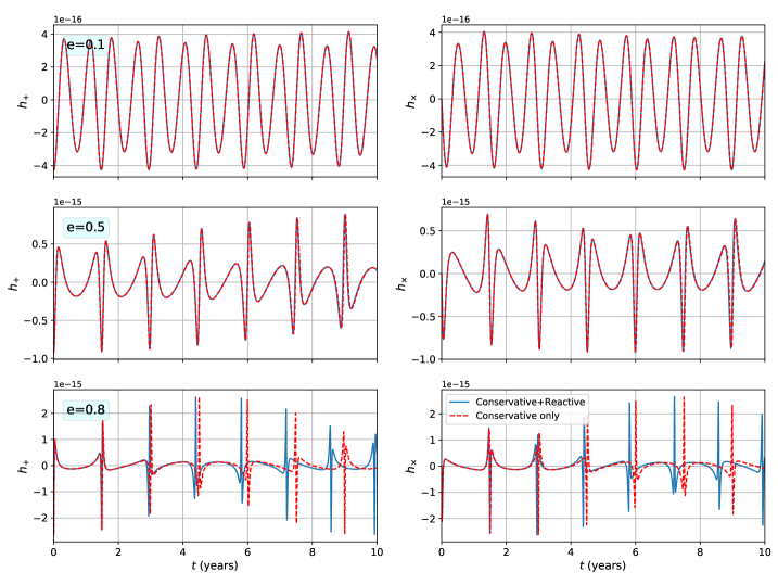
Figure 1: Temporally evolving $h_{+,\times}^{Q}$, namely quadrupolar order GW polarization states, associated with massive BH binaries in 3PN-accurate eccentric orbits. The sold line plots incorporate the effects of GW emission that enter the binary BH dynamics at the 2.5PN order and we ignore the effects of gravitational radiation reaction in the dashed line plots. We let $M=10^{9}M_{\astrosun}$, $\eta=0.25$, $D_{L}=1$ Gpc, $P_{b}=1.5$ years, $i=0$ and $\psi=0$ while selecting three $e_{t}$ values (the listed $e_{t}$ values provide orbital eccentricities at $t_{E}=0$ epoch in all our figures). The periapsis advance-induced amplitude modulations are clearly visible in the plots for moderately high to high eccentric binaries while GW emission-induced chirping is apparent in the $e=0.8$ plots.

Clearly, we need a prescription to include the effects of GW emission to model $h_{+,\times}(t)$ for compact binaries inspiraling along PN-accurate eccentric orbits. This is pursued by adapting the GW phasing formalism of Damour2006,KonigsdorfferGopakumar2006,Refs. Ref. Damour et al. (2004); Königsdörffer and Gopakumar (2006). This formalism demonstrated that GW emission forces $n$ and $e_{t}$ to change with time and it is possible to split their temporal evolution into two parts Damour et al. (2004). The first part leads to the secular or orbital-averaged evolution equations for $n$ and $e_{t}$ which ensure that both $n$ and $e_{t}$ can change substantially over the gravitational radiation reaction timescale. The second part essentially provides periodic variations to $n$ and $e_{t}$ in the orbital timescale, which remain tiny during the early inspiral phase of compact binary evolution Damour et al. (2004). Therefore, we ignore such periodic variations to $n$ and $e_{t}$ for the present investigation as our focus is indeed on the early part of the BH binary inspiral. The secular evolution of $n$ and $e_{t}$ ensures that $l$ and $\gamma$ no longer follow linear-in-time variations as noted earlier. With the inclusion of gravitation radiation reaction effects, the explicit temporal evolution for $l$ and $\gamma$ becomes

$$l-l_{0} =\int_{t_{0}}^{t}n(t^{\prime})\,dt^{\prime}\,,$$ (16a)

$$\gamma-\gamma_{0} =\int_{t_{0}}^{t}k(t^{\prime})n(t^{\prime})\,dt^{\prime}\,,$$ (16b)

where we have ignored orbital timescale variations in these angular variables Damour et al. (2004). These considerations imply that the GW phasing formalism provides a set of coupled differential equations for $n$, $e_{t}$, $\gamma$, and $l$. The resulting set of four coupled ordinary differential equations (ODEs) that incorporate secular effects of quadrupolar order GW emission read Damour et al. (2004),

$$\frac{dn}{dt} =\frac{1}{5}\left(\frac{GM_{\text{ch}}n}{c^{3}}\right)^{\frac{5}{3}}n^{2}\frac{\left(96+292e_{t}^{2}+37e_{t}^{4}\right)}{\left(1-e_{t}^{2}\right)^{7/2}}\,,$$ (17a)

$$\frac{de_{t}}{dt} =\frac{-1}{15}\left(\frac{GM_{\text{ch}}n}{c^{3}}\right)^{\frac{5}{3}}ne_{t}\frac{\left(304+121e_{t}^{2}\right)}{\left(1-e_{t}^{2}\right)^{5/2}}\,,$$ (17b)

$$\frac{d\gamma}{dt} =k\,n\,,$$ (17c)

$$\frac{dl}{dt} =n\,,$$ (17d)

where $M_{\text{ch}}=\eta^{3/5}M$ is the chirp mass of the binary. Note that we are required to solve the above set of four differential equations along with 3PN-accurate expressions for $u$ and $\phi$, given by Eqs. (13) and (14) to describe the orbital phase evolution of compact binaries inspiraling along 3PN-accurate eccentric orbits. In the next subsection, we develop a method to tackle these coupled differential equations in an essentially semi-analytic way.

II.3 Semi-analytic description for $n(t)$, $e_{t}(t)$, $\gamma(t)$, and $l(t)$

We begin by describing our computationally efficient way to obtain $n(t)$ and $e_{t}(t)$, influenced by Damour2006,Moore2018,Refs. Ref. Damour et al. (2004); Moore et al. (2018). Our approach involves deriving certain analytic expressions for $n(e_{t})$ and $t(e_{t})$ and appropriately treating them numerically to obtain an accurate and efficient way to track the temporal evolution in $n(t)$ and $e_{t}(t)$. To obtain an analytic expression for $n(e_{t})$, we divide Eq. (17a) by Eq. (17b), and this leads to

$$\frac{dn}{de_{t}}=-3\frac{n}{e_{t}}\frac{1}{\left(1-e_{t}^{2}\right)}\frac{\left(96+292e_{t}^{2}+37e_{t}^{4}\right)}{\left(304+121e_{t}^{2}\right)}\,.$$ (18)

It is easy to integrate the above equation to obtain

$$n(e_{t})=n_{0}\left(\frac{e_{t0}}{e_{t}}\right)^{\frac{18}{19}}\left(\frac{1-e_{t}^{2}}{1-e_{t0}^{2}}\right)^{\frac{3}{2}}\left(\frac{304+121e_{t0}^{2}}{304+121e_{t}^{2}}\right)^{\frac{1305}{2299}}\,,$$ (19)

where $n_{0}$ and $e_{t0}$ are the values of $n$ and $e_{t}$ at some initial epoch $t=t_{0}$ Damour et al. (2004). Unfortunately, it is not easy to obtain such a compact expression for $e_{t}(t)$. To obtain an equation that can be analytically tackled, we substitute the above equation for $n(e_{t})$ in Eq. (17b). The resulting equation may be written as

$$\frac{de_{t}}{dt}=-\kappa\,\frac{\left(1-e_{t}^{2}\right)^{3/2}}{e_{t}^{29/19}\left(121e_{t}^{2}+304\right)^{1181/2299}}\,,$$ (20a)

where

$$\kappa=\frac{1}{15}\left(\frac{GM_{\text{ch}}n_{0}}{c^{3}}\right)^{\frac{5}{3}}\frac{n_{0}e_{t0}^{\frac{48}{19}}\left(121e_{t0}^{2}+304\right)^{\frac{3480}{2299}}}{\left(1-e_{t0}^{2}\right)^{4}}\,.$$ (20b)

Note that the coefficient $\kappa$ is only a function of certain intrinsic binary BH parameters like the chirp mass, initial values of the mean motion and orbital eccentricity. Further, it is not difficult to infer that $\kappa$ has the dimensions of frequency and is non-zero for eccentric binaries. These considerations influenced us to introduce a dimensionless temporal parameter $\tau$ such that $\tau=\tau_{0}-\kappa\left(t-t_{0}\right)$, and Eq. (20a) in terms of $\tau$ becomes

$$\frac{de_{t}}{d\tau}=\frac{\left(1-e_{t}^{2}\right)^{3/2}}{e_{t}^{29/19}\left(121e_{t}^{2}+304\right)^{1181/2299}}\,,$$ (21)

and we will clarify the significance of the constant $\tau_{0}$ later. Interestingly, this equation does not contain any intrinsic (and constant) binary BH parameters. In other words, the above equation is valid for all eccentric compact binaries while restricting the GW emission effects to the leading quadrupolar order. It turns out that it is possible to obtain an analytical solution for Eq. (21), as noted in Moore2018,Refs. Ref. Moore et al. (2018), and it reads

$$\tau(e)=\frac{e^{\frac{48}{19}}}{768}\,\text{F}_{1}^{\text{A}}\left(\frac{24}{19};\frac{-1181}{2299},\frac{3}{2};\frac{43}{19};\frac{-121e^{2}}{304},e^{2}\right)\,,$$ (22)

where $\text{F}_{1}^{\text{A}}$ represents Appell’s 2D hypergeometric function Colavecchia et al. (2001), and we have chosen the initial condition $\tau(0)=0$ so that the constant of integration vanishes. It is indeed computationally very expensive to invert the above expression to get $e_{t}(\tau)$, mainly due to the difficulty in computing $\text{F}_{1}^{\text{A}}$ numerically. Therefore, we pre-compute $e_{t}(\tau)$ at a sufficiently dense set of points and interpolate between those points to get $e_{t}(\tau)$ for arbitrary values of $\tau$. Such a look-up table of $e_{t}(\tau)$ may be obtained either by numerically solving Eq. (21) or by inverting Eq. (22). The resulting $e_{t}(\tau)$ plot is displayed in Fig. 2 and it is important to note that GW emission forces $e_{t}$ to advance from right to left in our $e_{t}(\tau)$ plot. This is essentially due to the way $\tau$ is related to the coordinate time $t$, namely $\tau=\tau_{0}-\kappa\left(t-t_{0}\right)$. We have verified that our $e_{t}(\tau)$ evolution is consistent with Eq. (51) of Moore2018,Refs. Ref. Moore et al. (2018).

We note here that the frequency $n\rightarrow\infty$ as $e_{t}\rightarrow 0$ as evident from Eq. (19) and it influenced us to define certain merger time in our 2.5PN approximation as the instant when $e_{t}\rightarrow 0$. We are now in a position to explain the meaning of $\tau_{0}$ and for this purpose, we define certain dimensionless merger time by invoking the initial condition $\tau(0)=0$. This allows us to specify the above undetermined constant as $\tau_{0}=\tau(e_{t0})$, where $\tau(e_{t})$ is given by Eq. (22). We identify $\tau_{0}$ as certain dimensionless merger time because it is possible to compute certain ‘Newtonian’ merger time for compact binaries with its help. The relevant expression for such a merger time is given by

$$t_{\text{merg}}^{\text{2.5PN}}=\frac{\tau_{0}}{\kappa}\,,$$ (23)

and we have verified that this expression, in the small eccentricity limit, is indeed consistent with Eq. (50) of Krolak1995,Refs. Ref. Królak et al. (1995). Recall that Krolak1995,Refs. Ref. Królak et al. (1995) computed the ‘Newtonian merger time’ for compact binaries that incorporates the leading order eccentricity contributions as

$$\lim_{e_{0}\rightarrow 0}t_{\text{merg}}^{\text{2.5PN}}\sim\frac{5}{n_{0}}\left(\frac{GM_{\text{ch}}n_{0}}{c^{3}}\right)^{-\frac{5}{3}}\left(\frac{1}{256}-\frac{157e_{0}^{2}}{11008}\right)\,.$$ (24)

Additionally, we have computed an equivalent expression for such a merger time in Appendix B while clarifying our way to treat the $\kappa\rightarrow 0$ scenario.

Note that as a binary BH approaches the $\tau=0$ epoch, its orbital dynamics becomes more relativistic and this eventually leads to the breakdown of the present quadrupolar (or 2.5PN) order description of the binary BH reactive dynamics. Therefore, our prescription should only be used for an observational duration $t-t_{0}$ which is substantially smaller than $t_{\text{merge}}^{\text{2.5PN}}$. It turns out that our fully 3PN-accurate orbital description that incorporates the effects of quadrupolar order GW emission is quite appropriate while dealing with the expected isolated SMBH binary PTA sources.

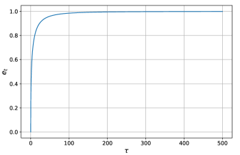
Figure 2: Numerical solution of Eq. (21) that provides $e_{t}(\tau)$ . Note that the dimensionless temporal variable $\tau$ is defined as $\tau\equiv\tau_{0}-\kappa(t-t_{0})$ and this is why a compact binary evolves from right to left along the $\tau$ axis. Let us emphasize that this curve defines the orbital eccentricity evolution for all compact binaries and the origin provides certain Newtonian merger epoch.

We now turn our attention to the evolution equations for $\gamma$ and $l$, given by Eqs. (17c) and (17d). The plan is to express both $n$ and $k\,n$ in terms of $e_{t}$, $n_{0}$ and $e_{0}$ with the help of our $n(e_{t})$ expression. Further, we employ our $\tau$ variable rather than its coordinate time ($t$) counterpart. This leads to

$$\frac{dl}{d\tau} =-\alpha\frac{\left(1-e_{t}^{2}\right)^{\frac{3}{2}}}{e_{t}^{\frac{18}{19}}\left(304+121e_{t}^{2}\right)^{\frac{1305}{2299}}}\,,$$ (25a)

$$\frac{d\gamma}{d\tau} =-\beta\frac{\left(1-e_{t}^{2}\right)^{\frac{3}{2}}}{e_{t}^{\frac{30}{19}}\left(304+121e_{t}^{2}\right)^{\frac{2175}{2299}}}\,,$$ (25b)

where the dimensionless coefficients $\alpha$ and $\beta$ are given by

$$\alpha =\left(\frac{GM_{\text{ch}}n_{0}}{c^{3}}\right)^{-\frac{5}{3}}\frac{15\left(1-e_{t0}^{2}\right){}^{5/2}}{e_{t0}^{\frac{30}{19}}\left(121e_{t0}^{2}+304\right)^{\frac{2175}{2299}}}\,,$$ (26a)

$$\beta =\left(\frac{GM_{\text{ch}}n_{0}}{c^{3}}\right)^{-\frac{5}{3}}\left(\frac{GMn_{0}}{c^{3}}\right)^{\frac{2}{3}}\frac{45\left(1-e_{t0}^{2}\right){}^{3/2}}{e_{t0}^{\frac{18}{19}}\left(121e_{t0}^{2}+304\right)^{\frac{1305}{2299}}}\,.$$ (26b)

It should be noted that we have only used the dominant order contributions to $k$, namely $k=3\,x/(1-e_{t}^{2})$, while obtaining the above equation for $d\gamma/dt$. Its 3PN extension is provided in Appendix A.

The next step is to obtain differential equations for $l$ and $\gamma$ that are independent of binary BH intrinsic (and constant) parameters. To this end, we define two scaled and shifted variables $\bar{l}=L_{0}-l/\alpha$ and $\bar{\gamma}=\Gamma_{0}-\gamma/\beta$. Invoking Eqs. (25a) and (25b), it is fairly straightforward to obtain the following differential equations for $\bar{l}$ and $\bar{\gamma}$

$$\frac{d\bar{l}}{d\tau} =\frac{\left(1-e_{t}^{2}\right)^{\frac{3}{2}}}{e_{t}^{\frac{18}{19}}\left(304+121e_{t}^{2}\right)^{\frac{1305}{2299}}}\,,$$ (27a)

$$\frac{d\bar{\gamma}}{d\tau} =\frac{\left(1-e_{t}^{2}\right)^{\frac{3}{2}}}{e_{t}^{\frac{30}{19}}\left(304+121e_{t}^{2}\right)^{\frac{2175}{2299}}}\,,$$ (27b)

with the following initial conditions ${l}(\tau_{0})=l_{0}$ and ${\gamma}(\tau_{0})=\gamma_{0}$. These initial conditions imply that the shifts $L_{0}$ and $\Gamma_{0}$ are given by

$$L_{0} =\bar{l}(\tau_{0})+\frac{l_{0}}{\alpha}\,,$$ (28a)

$$\Gamma_{0} =\bar{\gamma}(\tau_{0})+\frac{\gamma_{0}}{\beta}\,.$$ (28b)

The structure of the above two differential equations support analytic solutions if we compute $d\bar{l}/de_{t}$ and $d\bar{\gamma}/de_{t}$ versions of Eqs. (27a) and (27b) with the help of Eq. (21) for $de_{t}/d\tau$. This results in

$$\frac{d\bar{l}}{de_{t}} =\frac{e_{t}^{11/19}}{\left(121e_{t}^{2}+304\right)^{124/2299}}\,,$$ (29a)

$$\frac{d\bar{\gamma}}{de_{t}} =\frac{e_{t}^{-1/19}}{\left(121e_{t}^{2}+304\right)^{994/2299}}\,.$$ (29b)

The fact that the RHS of these equations depend only on $e_{t}$ allows us to obtain the following expressions for $\bar{l}$ and $\bar{\gamma}$

$$\bar{l}(e_{t}) =\frac{19^{\frac{2175}{2299}}}{30\times 2^{\frac{496}{2299}}}e_{t}^{\frac{30}{19}}\,{}_{2}\text{F}_{1}\left(\frac{124}{2299},\frac{15}{19};\frac{34}{19};\frac{-121e_{t}^{2}}{304}\right),$$ (30a)

$$\bar{\gamma}(e_{t}) =\frac{19^{\frac{1305}{2299}}}{36\times 2^{\frac{1677}{2299}}}e_{t}^{\frac{18}{19}}\,{}_{2}\text{F}_{1}\left(\frac{994}{2299},\frac{9}{19};\frac{28}{19};\frac{-121e_{t}^{2}}{304}\right),$$ (30b)

where ${}_{2}\text{F}_{1}$ is the Gaussian hypergeometric function, and we have verified that the above expression for $\bar{l}$ is consistent with Eq. (52) of Moore2018,Refs. Ref. Moore et al. (2018). In Figure 3, we plot these variables against $e_{t}$ and find the expected sharp rise in $\bar{l}$ for higher orbital eccentricities. It is important to note that these plots are independent of the intrinsic (and constant) binary BH parameters like the total mass, mass ratio, and initial orbital eccentricity and period.

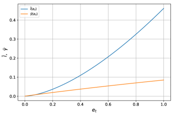
Figure 3: The non-linear variation of our two scaled angular variables $\bar{l}$ and $\bar{\gamma}$ as function of $e_{t}$. The use of these variables ensures that such variations are system independent at the quadrupolar order GW emission.

To obtain the actual temporal evolution for the above set of variables, namely $n$, $e_{t}$, $l$ and $\gamma$, we proceed as follows. First, we compute a look-up table for $e_{t}(\tau)$ by solving the the differential equation for $de_{t}/d\tau$ as described earlier. We emphasize here that this is a one-time computation since the differential equation (21) does not contain any system-dependent parameters, which implies that the look-up table, once computed, may be saved and re-used for later computations. (Details of this computation are given in subsection II.3.1.) Thereafter, we determine $n(\tau)$, $l(\tau)$, and $\gamma(\tau)$ with the help of Eqs. (19), (30a), and (30b) that involve hypergeometric functions. Using the explicit expressions for $\tau_{0}$, $\kappa$, $\alpha$, and $\beta$ and specific relations that connect $\tau$ to $t$, $\bar{l}$ to $l$, and $\bar{\gamma}$ to $\gamma$, it is straightforward to obtain binary BH system-dependent temporal evolution for $n$, $e_{t}$, $l$, and $\gamma$ in terms of the regular coordinate time $t$. Let us emphasize that these variable changes are easy to implement as they essentially involve analytic expressions. To ascertain the accuracy of this procedure, we compared $n(t)$, $e_{t}(t)$, $\gamma(t)$ and $l(t)$ computed using this method to results obtained by numerically solving the system of ODEs (17) for different initial conditions, masses and mass ratios. We find that the results agree up to the numerical precision of the ODE solver as expected.

The variables $u$ and $\phi$ which appear in the waveform (7) may be computed using Eqs. (13-14). Finally, the PTA signal $R(t)$ can be computed by numerically integrating the waveform as given by Eqs. (3-6). We are forced to perform this integral numerically owing to the fact that the waveform (7) is a function of $u$ and $\phi$ which are not simple functions of the coordinate time.

II.3.1 Computation of $e_{t}(\tau)$

Clearly, an accurate and efficient prescription to obtain $e_{t}(\tau)$ is crucial for describing the temporal evolution of ($n,e_{t},\gamma,l$) in terms of the coordinate time $t$. The fact that an explicit expression is available only for $\tau(e_{t})$ and not for $e_{t}(\tau)$ forced us to obtain $e_{t}(\tau)$ either by numerically integrating Eq. (21) or by numerically inverting the analytic expression for $\tau(e_{t})$ given by Eq. (22). However, we pursued the relatively computationally inexpensive approach of computing a look-up table for $e_{t}(\tau)$ at a sufficiently dense sample of $\tau$ values for one time. Thereafter, we obtain values of $e_{t}(\tau)$ at arbitrary $\tau$ values by interpolating between the pre-computed values and this is heavily influenced by the universal nature of Eq. (21). In practice, we solve Eq. (21) using an adaptive ODE solver, which adjusts the step size to ensure an optimal accuracy of the solution while constructing the look-up table. This is important as the curvature of the function $e_{t}(\tau)$ is highly variable, as evident from Fig. (2). Therefore, the look-up table must be computed at a non-uniform sample of points such that the regions of high curvature are sampled at sufficiently high density for ensuring high accuracy.

This approach poses a new challenge since our $de_{t}/d\tau$ equation diverges at $e_{t}=0$ as evident from Eq. (21). This implies that the numerical integration cannot start with the expected initial condition, namely $e_{t}(0)=0$. We avoid this issue by starting the numerical integration at a small non-zero value of $\tau$, say certain $\tau_{\min}$. To compute such an initial condition $e_{t}(\tau_{\min})$, we explore the asymptotic $(\tau,e_{t})\rightarrow(0,0)$ behaviour of Eq. (21). In this limit, Eq. (21) becomes

$$\lim_{\tau,e_{t}\rightarrow 0}\frac{de_{t}}{d\tau} \sim\frac{1}{304^{\frac{1181}{2299}}e_{t}^{\frac{29}{19}}}\,,$$ (31)

where we have expanded the R.H.S. of Eq. (21) to the leading order contributions in $e_{t}$. This equation can be integrated to obtain

$$\lim_{\tau\rightarrow 0}e_{t}(\tau) \sim\frac{2^{559/726}3^{19/48}}{19^{145/242}}\tau^{19/48}\,.$$ (32)

Therefore, the new initial condition becomes

$$e_{t,\min}=\frac{2^{559/726}3^{19/48}}{19^{145/242}}\tau_{\min}^{19/48}\,,$$ (33)

for some sufficiently small $\tau_{\min}$. The look-up table for $\tau(e)$ can now be computed by integrating Eq. (21) from $\tau_{\min}$ to some $\tau_{\max}$ such that it covers all eccentricity values of interest.

It is also possible to provide an estimate for $\tau_{\max}$ where we can stop the numerical integration. Using the fact that $\lim_{\tau\rightarrow\infty}e_{t}=1$, we write Eq. (21) in the $\tau\rightarrow\infty$ limit as

$$\lim_{\tau\rightarrow\infty}\frac{d\epsilon}{d\tau} \sim\frac{2\sqrt{2}\,\epsilon^{3/2}}{5\ 5^{63/2299}17^{1181/2299}}\,,$$ (34)

where we have substituted $\epsilon=1-e_{t}$ in Eq. (21) and expanded the R.H.S. of the resulting equation to the leading order in $\epsilon$. This equation can be solved fairly easily to obtain

$$\lim_{\tau\rightarrow\infty}e_{t} \sim 1-\frac{4}{(a\tau+b)^{2}}\,,$$ (35)

where we have defined the coefficient

$$a =\frac{2\sqrt{2}}{5\times 5^{63/2299}17^{1181/2299}}\,.$$ (36)

In contrast, the coefficient $b$ may be computed by imposing the initial condition $e_{t}(\tau_{\max})=e_{t,\max}$ to be

$$b =\frac{2}{\sqrt{1-e_{t,\max}}}-a\tau_{\max}\,.$$ (37)

In our approach, we provide these limits to obtain an accurate and efficient prescription to evaluate $e_{t}(\tau)$.  

We are now in a position to obtain the PTA signals due to massive BH binaries inspiraling along 3PN-accurate eccentric orbits, and this is what we explore in the next subsection.

II.4 Pictorial exploration of $R(t)$ due to BH binaries in relativistic eccentric orbits

We begin by displaying temporally evolving quadrupolar order $h_{+,\times}^{Q}(t)$, specified by Eqs. (7), while employing our semi-analytic prescription for evolving $n$, $e_{t}$, $\gamma$, and $l$ in Fig. 1. It should be noted that our explicit expressions for $h_{+,\times}^{Q}$ involve $u$ and therefore, we additionally need to invert the 3PN-accurate Kepler Equation, given by Eq. (13), at every $l$ value to obtain the temporal evolution of our dominant order GW polarization states. The treatment of PN-accurate Kepler Equation, as noted earlier, is performed by adapting and extending the Mikkola’s method Mikkola (1987); Tessmer and Gopakumar (2007). The resulting $h_{+,\times}(t)$ associated with massive BH binaries inspiraling along fully 3PN-accurate eccentric orbits are displayed in Fig. 1, and are labelled “Conservative+Reactive”. The effects of GW emission are clearly visible in $e=0.8$ plots and it causes certain waveform dephasing while comparing with plots that do not include the effects of GW emission. Let us emphasize that our semi-analytic approach is capable of treating orbital eccentricities that are $\leq 1$ as we explicitly employ the eccentric anomaly $u$ to trace the PN-accurate eccentric orbit.

We now have all the ingredients to obtain ready-to-use PTA signals associated with non-spinning SMBH binaries inspiraling along PN-accurate eccentric orbits. As mentioned earlier, the fact that $h_{+,\times}^{Q}$ expressions given by Eqs. (7) explicitly contain $u$ and $\phi$ prevents us from evaluating analytically the integrals that appear in the expression for $R(t)$ as evident from Eqs. (4-6). Therefore, we employ an adaptive numerical integration routine, namely the QAG routine Zwillinger (1992) to evaluate Eqs. (4-6) while computing pulsar timing residuals. We first provide a pictorial depiction of $R(t)$ and explain its various features with the help of $+/\times$ residual plots.

We display in Fig. 4 PTA signals induced on PSR J0437$-$4715 by a fiducial equal mass BH binary having $M=10^{9}\,M_{\astrosun}$ with face-on orbit ($i=0$) at a luminosity distance of $1$ Gpc, for three different eccentricities and two different orbital periods. We let the sky location of the GW source to be RA $08^{h}00^{m}00^{s}$, DEC $-20^{\circ}00^{\prime}00^{\prime\prime}$, with $\psi=0$. Each panel in Fig. 4 corresponds to a particular combination of orbital eccentricity and orbital period at the $t_{E}=0$ epoch. Additionally, we choose two estimates for the pulsar distance, namely 156.79 pc and 157.04 pc, which are consistent with the $1\sigma$ uncertainty for its measurement, available in Reardon2016,Refs. Ref. Reardon et al. (2016). These choices lead to two plots each in six panels of Fig. 4. Amplitude modulations, visible in the moderate to high eccentricity cases for $P_{b}=1.5$ yrs, are due to the fact that the pulsar term contributions can have substantially different orbital eccentricity and period for such high eccentric systems. Interestingly, temporal evolution of $R(t)$ is pulsar distance-dependent especially for the lower and moderate $e$ values as evident from the first two panels for $P_{b}$=1.5 yrs. Prominent dephasing in the $P_{b}$=1.5 yrs case may be due to the fact that the change in pulsar distance is roughly equivalent to half of the orbital period. Such changes in the $R(t)$ evolution is less pronounced for the high $e$ case as the underlying frequencies of the Earth and pulsar terms are significantly different. In contrast, such strong dependence of $R(t)$ on the pulsar distance is not observed in the $P_{b}$=5 yrs case due to the fact that the pulsar distance difference is not tuned to the orbital period. Interestingly, the epochs of the sharp features, visible in Fig. 4, are very sensitive to the pulsar distance in the $P_{b}$=1.5 yrs case, and its implications are being investigated.

To get a pulsar-independent view of these timing residuals, we plot in Fig. 5 the associated $+/\times$ residuals while separating the Earth and the Pulsar term contributions using identical parameters to Fig. 4, with $P_{b}=5$ yrs. These plots confirm our earlier statement that the pulsar term, which provides a snapshot of the orbital configuration of our GW source at an earlier epoch, can have substantially different orbital eccentricity and period, especially for highly eccentric BH binaries. It is clearly the mixing of the two contributions with very different evolution timescales that produces various features present in our $R(t)$ plots.

We now proceed to display the quadrupolar nature of our PTA signal in Fig. 6. Specifically, we plot certain strength of the Earth term as a function of the sky location of the pulsar for a given GW source. This strength of the Earth term is defined as the difference between the maximum and minimum of $s(t_{E})$ within a given time span. The top and bottom panels show such $s(t_{E})$ strength for $\psi=0$ and $\psi=45^{\circ}$ values, respectively. For these plots, we let the orbital eccentricity of the GW source to be 0.5 and the all other parameters are same as in Fig. 4 and Fig. 5. Our plots clearly show the quadrupolar pattern of the expected PTA signal, and the comparison between the top and bottom panels reveals the $45^{\circ}$ rotation that is expected from the $\psi$ values. Additionally, these plots essentially confirm that we are employing appropriate expressions for $F_{\times}$ and $F_{+}$.

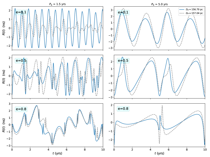
Figure 4: PTA signals induced on PSR J0437$-$4715 by a fiducial massive BH binary at $1$ Gpc away with two different $P_{b}$ values and three $e_{t}$ values at $t_{E}=0$ epoch. The location of this pulsar is given by RA $04^{h}37^{m}16^{s}$, DEC $-47^{\circ}15^{\prime}09^{\prime\prime}$ and is at a distance of 156.79 pc Reardon et al. (2016). The sky location of the binary is arbitrarily chosen to be RA $08^{h}00^{m}00^{s}$, DEC $-20^{\circ}00^{\prime}00^{\prime\prime}$ and other binary parameters are the same as in Fig. 5. The dashed plots correspond to a pulsar distance of 157.04 pc, which is off from the measured distance by its $1\sigma$ uncertainty Reardon et al. (2016). It is very clear that the features of $R(t)$ for $P_{b}=1.5$ yrs are very sensitive to the pulsar distance, especially for low and moderate eccentricities. This may be attributed to the frequencies of the Earth and pulsar terms being similar for low and moderate eccentricities and the pulsar distance difference being roughly equivalent to half the orbital period. In contrast, the features of the $P_{b}=5$ yrs case are much less sensitive to the pulsar distance as the pulsar distance difference is not tuned to the orbital period.

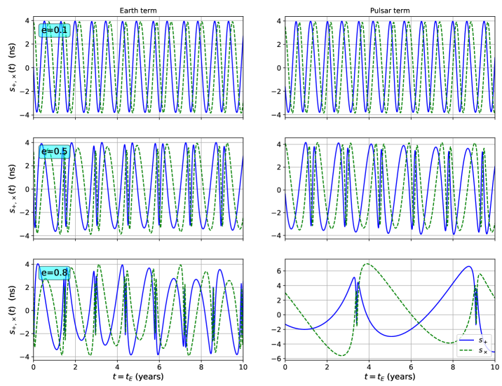
Figure 5: Plots of $s_{+,\times}(t)$, namely the plus/cross residuals, for a $1$ Gpc away equal mass binary BH having different orbital eccentricities at the initial Earth epoch while all other binary parameters are similar to those in Fig. 1 with $P_{b}=1.5$ yrs at $t_{E}=0$. We plot both the Earth and the Pulsar term contributions while assuming a geometric delay of $1000$ years between these two locations. The GW emission ensures that fiducial pulsar contributions to $s_{+,\times}(t)$ have higher orbital eccentricities and periods. This is very prominent for the large initial eccentricity ($e=0.8$) binary BH configuration.

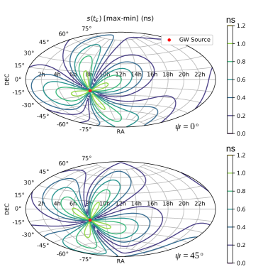
Figure 6: Graphical display of the ‘strength’ of the Earth term $s(t_{E})$ as a function of pulsar’s sky location. The two panels are for two specific values of GW polarization angle and the rest of the parameters are identical to those employed in Fig. 4 with $P_{b}=1.5$ yrs at $t_{E}=0$. In these plots, the red dot represents the sky location of the GW source and the expected quadrupolar pattern is clearly visible. We rotate the bottom panel plot by $45^{\circ}$ w.r.t the top panel plot in accordance with the $\psi$ values used.

We now turn our attention towards the numerical costs of our approach to obtain the temporal evolution of $n$, $e_{t}$, $\gamma$, and $l$ as well as the computation of the PTA signal $R(t)$, and this is what we explore in the next subsection.

II.5 The cost of computing the orbital evolution and the PTA signal

We begin by comparing the computational cost of our semi-analytic approach against numerically solving Eqs. (17) to obtain the orbital evolution. Excluding the one-time cost of computing the look-up table for $e(\tau)$, the execution time $t^{\text{exec}}$ taken to compute the state of the orbit $(n,e_{t},\gamma,l)$ at a given set of TOAs should depend on the number of TOAs ($N_{\text{TOA}}$) as well as their total observation span/integration span (specified by some $t_{0}$ and $t_{1}$). This is illustrated in the top panel of Fig. 7 where we plot the execution time per TOA ($t^{\text{exec}}/N_{\text{TOA}}$) required to compute our variables $(n,e,\gamma,l)$ as a function of $N_{\text{TOA}}$ for different integration spans ($t_{1}-t_{0}$) in our semi-analytic approach. This panel shows that the computational time required for evaluating $(n,e,\gamma,l)$ at a given TOA is independent of both the integration span as well as the number of TOAs when the number of TOAs is sufficiently large. This impressive feature may be contrasted with the fact that the execution time, when TOA numbers are small, is dominated by the one-time evaluation of various coefficients like $\kappa$, $\alpha$ and $\beta$.

The bottom panel of Fig. 7 compares the performance gain of our semi-analytic method with respect to the usual approach of solving numerically Eqs. (17) by employing the ratio of execution times ($t_{\text{num}}^{\text{exec}}/t_{\text{anl}}^{\text{exec}}$). The associated plots reveal that this ratio increases substantially as one increases the integration span, especially for low $N_{\text{TOA}}$ values. However, the ratio eventually decreases and essentially converges to a value close to $5$ when $N_{\text{TOA}}$ is a large number. This behavior is expected, since a numerical ODE solver is required to compute the right hand side of Eqs. (17) at many points between the TOAs where the solutions are required while evolving the binary over time. In contrast, our semi-analytic approach only computes the solutions at the required TOAs. However, as the number of TOAs within an integration span increases, the number of intermediate points required by the numerical solver decreases too. This leads to the behavior displayed in the bottom panel of Fig. 7, and we infer that the semi-analytic solution usually outperforms the numerical one.

Fig. 8 shows the time taken to compute the PTA signal $R(t)$ per TOA ($t^{\text{exec}}_{\text{signal}}/N_{\text{TOA}}$) as a function of $N_{\text{TOA}}$ for different integration spans. Once again, we see that the execution time is dominated by the one-time computations when $N_{\text{TOA}}$ is small, but is independent of $N_{\text{TOA}}$ when $N_{\text{TOA}}$ is large. A comparison of Fig. 8 with the top panel of Fig. 7 reveals that the execution time of computing $R(t)$ is dominated by the cost of numerically integrating $h(t)$ to get $R(t)$.

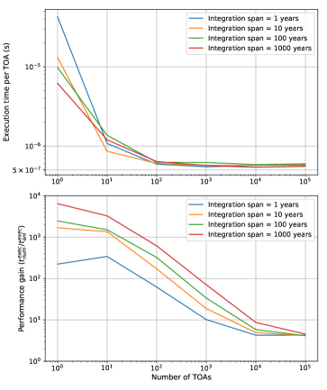
Figure 7: Plots that compare execution times associated with the evolution of an eccentric binary using two approaches. The numerical approach (num) solves the set of four differential equations, given by Eqs. (17), by employing the gsl_odeiv2_step_rkf45 adaptive integration method of the GNU Scientific Library (GSL). The special functions, required by our analytic approach, are also evaluated with the help of GSL. We consider equal mass BH binaries with $M=10^{9}\,M_{\astrosun}$, $P_{b0}=1.5$ years, $e_{t0}=0.5$, and let $l_{0}=\gamma_{0}=0$. These computations were performed in C++ in an Intel Core i7 machine using a single core. These plots reveal that our semi-analytic approach is more efficient that the regular numerical approach.

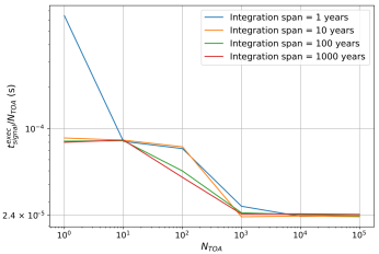
Figure 8: The execution time per TOA for computing $R(t)$. For small $N_{\text{TOA}}$ the execution time is dominated by one-time computations whereas for large $N_{\text{TOA}}$ it is essentially independent of $N_{\text{TOA}}$. A comparison with the top panel of Fig. 7 also reveals that the execution time is dominated by the numerical integration of $h(t)$ to compute $R(t)$.

Clearly, it is desirable to provide appropriate checks to verify the correctness of our detailed prescription for computing pulsar timing residuals, induced by relativistic eccentric binaries as it involves many numerical ingredients and detailed and lengthy analytic expressions. This is pursued in the next section where we provide a fully analytic way to compute $+/\times$ residuals for non-spinning BH binaries moving in PN-accurate moderately eccentric orbits.

III Fully analytic $+/\times$ residuals for binaries in Post-Keplerian small-eccentricity orbits

This section provides a fully analytic way of computing pulsar timing residuals due to BH binaries moving in quasi-Keplerian orbits of moderate eccentricities. This effort invokes explicit analytic expressions for $h_{+,\times}^{Q}(t)$ that are associated with non-spinning compact binaries moving in conservative 3PN-accurate small eccentricity orbits, derived in Boetzel2017,Refs. Ref. Boetzel et al. (2017). The main motivation, as noted earlier, is to provide a powerful check on the results, originating from our semi-analytic approach, for computing $s_{+,\times}(t)$ associated with quasi-Keplerian orbits of arbitrary eccentricities. The present section is also influenced by Taylor2016,Refs. Ref. Taylor et al. (2016) that provided explicit analytic expressions for the quadrupolar order $+,\times$ residuals from BH binaries in Newtonian eccentric orbits.

The effort, detailed in Taylor2016,Refs. Ref. Taylor et al. (2016) , employs various results from the Fourier analysis of the classical Kepler equation in terms of the Bessel functions, available in Colwell1993,Refs. Ref. Colwell (1993) and apply them in the quadrupolar order $h_{+,\times}^{Q}$ expressions, given by Eqs. (7) Peters and Mathews (1963). The resulting fully analytic Newtonian GW polarization states may be symbolically written as Taylor et al. (2016)

$$h_{+}(t) =\sum_{p=0}^{\infty}\left(a_{p}^{+}\cos\left(pl\right)\cos\left(2\omega\right)\right.$$

$$\quad\quad\quad\left.+b_{p}^{+}\sin\left(pl\right)\sin\left(2\omega\right)+c_{p}^{+}\cos\left(pl\right)\right)\,,$$ (38a)

$$h_{\times}(t) =\sum_{p=0}^{\infty}\left(a_{p}^{\times}\cos\left(pl\right)\sin\left(2\omega\right)\right.$$

$$\quad\quad\quad\left.+b_{p}^{\times}\sin\left(pl\right)\cos\left(2\omega\right)\right)\,,$$ (38b)

where the coefficients $a_{p}^{+,\times}$, $b_{p}^{+,\times}$ and $c_{p}^{+}$ contain trigonometric functions of the orbital inclination $i$, while the orbital eccentricity $e_{t}$ enters in terms of Bessel functions of the first kind Moreno-Garrido et al. (1995). Recall that $\omega$ provides the argument of periapsis, which remains a constant for Newtonian orbits. This ensures that such Newtonian compact binaries emit GWs at frequencies that are integer harmonics of $n$. It is also possible to incorporate in an ad-hoc manner the linear-in-time evolution of $\omega$ to the above Newtonian order $h_{+,\times}$ expressions Seto (2001); Barack and Cutler (2004). Employing the above Newtonian order expressions for the two GW polarizations states, Taylor2016,Refs. Ref. Taylor et al. (2016) computed analytically the $+/\times$ residuals which may be written symbolically as

$$s_{+}(t) =\sum_{p=0}^{\infty}\frac{1}{np}\left(a_{p}^{+}\sin\left(pl\right)\cos\left(2\omega\right)\right.$$

$$\quad\quad\quad\left.-b_{p}^{+}\cos\left(pl\right)\sin\left(2\omega\right)+c_{p}^{+}\sin\left(pl\right)\right)\,,$$ (39a)

$$s_{\times}(t) =\sum_{p=0}^{\infty}\frac{1}{np}\left(a_{p}^{\times}\sin\left(pl\right)\sin\left(2\omega\right)\right.$$

$$\quad\quad\quad\quad\left.-b_{p}^{\times}\cos\left(pl\right)\cos\left(2\omega\right)\right)\,.$$ (39b)

The explicit form of these coefficients may be easily extracted with the help of Eqs. (21) and (22) of Taylor2016,Refs. Ref. Taylor et al. (2016). In what follows, we provide a fully post-Newtonian accurate version of these results.

Recall that fully analytic $h_{+,\times}^{Q}(l)$ expressions for compact binaries moving in conservative 3PN-accurate quasi-Keplerian small eccentric orbits were derived in Boetzel2017,Refs. Ref. Boetzel et al. (2017). This derivation employed Eqs. (7) for $h_{+,\times}^{Q}$ and an analytic treatment of the PN-accurate Kepler equation. The detailed analysis of Boetzel2017,Refs. Ref. Boetzel et al. (2017) provided PN-accurate expressions for both eccentric and true anomalies in terms of infinite series expressions involving $l$ and $e_{t}$. We write symbolically the resulting quadrupolar order $h_{+,\times}(l)$ expressions as

$$h_{+,\times}(t) =\sum_{p=0}^{\infty}\sum_{q=0}^{\infty}\left\{a_{p,q}^{+,\times}\cos\left(pl\right)\cos\left(q\lambda\right)\right.$$

$$\quad\quad\left.+b_{p,q}^{+,\times}\sin\left(pl\right)\cos\left(q\lambda\right)\right.$$

$$\quad\quad\left.+c_{p,q}^{+,\times}\cos\left(pl\right)\sin\left(q\lambda\right)\right.$$

$$\quad\quad\left.+d_{p,q}^{+,\times}\sin\left(pl\right)\sin\left(q\lambda\right)\,\right\}\,,$$ (40)

where we have defined $\lambda=l+\gamma$ Boetzel et al. (2017). A straightforward integration of the above expression leads to

$$s_{+,\times}(t) =\frac{1}{n}\sum_{p,q=0}^{\infty}{\vphantom{\sum}}^{\prime}\left\{A_{p,q}^{+,\times}\cos\left(pl\right)\cos\left(q\lambda\right)\right.$$

$$\qquad\left.+B_{p,q}^{+,\times}\sin\left(pl\right)\cos\left(q\lambda\right)\right.$$

$$\qquad\left.+C_{p,q}^{+,\times}\cos\left(pl\right)\sin\left(q\lambda\right)\right.$$

$$\qquad\left.+D_{p,q}^{+,\times}\sin\left(pl\right)\sin\left(q\lambda\right)\,\right\}\,,$$ (41)

where we have ignored the effects of GW emission while performing various integrations. This is justified as the radiation reaction timescale is substantially larger than the orbital and advance of periapsis timescales. Further, the primed sum excludes the $p=q=0$ term in the above expressions. These multi-index $A$, $B$, $C$, $D$ coefficients involve $x$, $\eta$, trigonometric functions of $i$, and $e_{t}$ contributions via infinite series of Bessel functions. They may be expressed as

$$A_{p,q}^{+,\times} =\frac{-p\,b_{p,q}^{+,\times}+(1+k)q\,c_{p,q}^{+,\times}}{p^{2}-(1+k)^{2}q^{2}}\,,$$ (42a)

$$B_{p,q}^{+,\times} =\frac{p\,a_{p,q}^{+,\times}+(1+k)q\,d_{p,q}^{+,\times}}{p^{2}-(1+k)^{2}q^{2}}\,,$$ (42b)

$$C_{p,q}^{+,\times} =\frac{-p\,d_{p,q}^{+,\times}-(1+k)q\,a_{p,q}^{+,\times}}{p^{2}-(1+k)^{2}q^{2}}\,,$$ (42c)

$$D_{p,q}^{+,\times} =\frac{p\,c_{p,q}^{+,\times}-(1+k)q\,b_{p,q}^{+,\times}}{p^{2}-(1+k)^{2}q^{2}}\,.$$ (42d)

Clearly, it is neither advisable nor feasible to evaluate these coefficients for arbitrarily high $p$ and $q$ values to high precision. This is because the underlying Bessel function evaluations are computationally very expensive. However, it is straightforward to obtain Taylor expansions of these coefficients around $e_{t}=0$. The resulting expansions, accurate up to some $\mathcal{O}(e_{t}^{m})$, ensure that the Fourier coefficients beyond a certain $p_{\max}$ and $q_{\max}$ vanish for any given $m$. This is essentially due to the following property of the Bessel functions of the first kind

$$\lim_{x\rightarrow 0}\text{J}_{m}(x)\sim\mathcal{O}(x^{m})\,.$$

Unfortunately, both the Fourier series, given by Eqs. (42) and the associated power series expansions for the involved $A$, $B$, $C$, $D$ coefficients converge slowly for moderately large $e_{t}$ values. This might signal the breaking down of the approximation and may be associated with the celebrated Laplace limit Watson (1966). Detailed comparisons of various Bessel function contributions, computed numerically and analytically, reveal that such an expansion accurate up to $\mathcal{O}(e_{t}^{8})$ can be used to compute timing residuals for eccentricities less than $0.3$. In what follows, we display the explicit expressions for the quadrupolar order $h^{Q}_{+}(l)$ that includes all the eccentricity corrections up to $\mathcal{O}(e_{t}^{4})$, and the associated $+$ residual:

$$h_{+}^{Q} ={\cal H}_{0}\Bigg{[}\left(e_{t}s_{i}^{2}-\frac{1}{8}e_{t}^{3}s_{i}^{2}\right)\cos(l)+\left(e_{t}^{2}s_{i}^{2}-\frac{1}{3}e_{t}^{4}s_{i}^{2}\right)\cos(2l)$$

$$\quad+\left(-\frac{1}{8}23e_{t}^{4}c_{i}^{2}+5e_{t}^{2}c_{i}^{2}-2c_{i}^{2}-\frac{23e_{t}^{4}}{8}+5e_{t}^{2}-2\right)\cos(2\lambda)$$

$$\quad+\left(\frac{1}{8}e_{t}^{4}c_{i}^{2}+\frac{e_{t}^{4}}{8}\right)\cos(4l-2\lambda)+\left(-\frac{1}{4}81e_{t}^{4}c_{i}^{2}-\frac{81e_{t}^{4}}{4}\right)\cos(2\lambda+4l)$$

$$\quad+\left(\frac{171}{16}e_{t}^{3}c_{i}^{2}-\frac{9e_{t}c_{i}^{2}}{2}+\frac{171e_{t}^{3}}{16}-\frac{9e_{t}}{2}\right)\cos(2\lambda+l)+\left(\frac{7}{48}e_{t}^{3}c_{i}^{2}+\frac{7e_{t}^{3}}{48}\right)\cos(3l-2\lambda)$$

$$\quad+\left(-\frac{1}{48}625e_{t}^{3}c_{i}^{2}-\frac{625e_{t}^{3}}{48}\right)\cos(2\lambda+3l)+\left(20e_{t}^{4}c_{i}^{2}-8e_{t}^{2}c_{i}^{2}+20e_{t}^{4}-8e_{t}^{2}\right)\cos(2\lambda+2l)$$

$$\quad+\left(-\frac{1}{16}13e_{t}^{3}c_{i}^{2}+\frac{3e_{t}c_{i}^{2}}{2}-\frac{13e_{t}^{3}}{16}+\frac{3e_{t}}{2}\right)\cos(l-2\lambda)+\frac{9}{8}e_{t}^{3}s_{i}^{2}\cos(3l)+\frac{4}{3}e_{t}^{4}s_{i}^{2}\cos(4l)\Bigg{]}\,,$$ (43a)

$$s_{+}^{Q} =\frac{{\cal H}_{0}}{n}\Bigg{[}\;\left(e_{t}s_{i}^{2}-\frac{1}{8}e_{t}^{3}s_{i}^{2}\right)\sin(l)+\left(\frac{1}{2}e_{t}^{2}s_{i}^{2}-\frac{1}{6}e_{t}^{4}s_{i}^{2}\right)\sin(2l)$$

$$\quad+\left(-\frac{1}{16}23e_{t}^{4}c_{i}^{2}+\frac{5}{2}e_{t}^{2}c_{i}^{2}-c_{i}^{2}-\frac{23e_{t}^{4}}{16}+\frac{5e_{t}^{2}}{2}-1\right)\sin(2\lambda)$$

$$\quad+\left(\frac{13}{16}e_{t}^{3}c_{i}^{2}-\frac{3e_{t}c_{i}^{2}}{2}+\frac{13e_{t}^{3}}{16}-\frac{3e_{t}}{2}\right)\sin(l-2\lambda)+\left(\frac{57}{16}e_{t}^{3}c_{i}^{2}-\frac{3e_{t}c_{i}^{2}}{2}+\frac{57e_{t}^{3}}{16}-\frac{3e_{t}}{2}\right)\sin(2\lambda+l)$$

$$\quad+\left(\frac{1}{16}e_{t}^{4}c_{i}^{2}+\frac{e_{t}^{4}}{16}\right)\sin(4l-2\lambda)+\left(-\frac{1}{8}27e_{t}^{4}c_{i}^{2}-\frac{27e_{t}^{4}}{8}\right)\sin(2\lambda+4l)$$

$$\quad+\left(\frac{7}{48}e_{t}^{3}c_{i}^{2}+\frac{7e_{t}^{3}}{48}\right)\sin(3l-2\lambda)+\left(-\frac{1}{48}125e_{t}^{3}c_{i}^{2}-\frac{125e_{t}^{3}}{48}\right)\sin(2\lambda+3l)$$

$$\quad+\left(5e_{t}^{4}c_{i}^{2}-2e_{t}^{2}c_{i}^{2}+5e_{t}^{4}-2e_{t}^{2}\right)\sin(2\lambda+2l)+\frac{1}{3}e_{t}^{4}s_{i}^{2}\sin(4l)+\frac{3}{8}e_{t}^{3}s_{i}^{2}\sin(3l)\;\Bigg{]}\,,$$ (43b)

where we have defined ${\mathcal{H}}_{0}=\frac{GM\eta}{D_{L}c^{2}}x$. We note in passing that we have explicitly computed the quadrupolar order $h_{+,\times}(l)$ and its temporally evolving $+/\times$ residuals that include all the $\mathcal{O}(e_{t}^{8})$ corrections. Additionally, these expressions were employed while making comparisons of our analytic and semi-analytic approaches to compute $s_{+,\times}(t)$, displayed in Fig. 9.

We are now in a position to use these expressions to test our involved semi-analytical approach to obtain $+/\times$ residuals valid for arbitrary eccentricities. In Fig. 9, we overlay plots of $s_{+,\times}^{Q}(t)$ that arise from the above mentioned analytic approach and our semi-analytic approach while focusing only on the Earth term for three initial values of $e_{t}$. Additionally, we let the orbital elements and angles to vary according to our improvised GW phasing approach, detailed in Sec. II.3, in both the approaches. We observe excellent agreement between the two approaches for initial $e_{t}$ values up to $0.3$ and it is difficult to distinguish the dashed line plots in the first two panels. Therefore, these plots give us the confidence about the correctness of our semi-analytic approach to obtain $R(t)$ for BH binaries inspiraling along relativistic eccentric orbits. However, our analytic post-circular approach becomes progressively worse for a larger initial $e$ value as evident from the bottom panel plots. We quantify the deviation between our semi-analytic and fully analytic temporally evolving plus/cross residuals with the help of the following normalized integrated error defined as

$$\varepsilon(e_{0})=\frac{\sum_{i}\left[\left(s_{+}^{\text{num}}(t_{i})-s_{+}^{\text{anl}}(t_{i})\right)^{2}+\left(s_{\times}^{\text{num}}(t_{i})-s_{\times}^{\text{anl}}(t_{i})\right)^{2}\right]}{\sum_{i}\left[\left(s_{+}^{\text{num}}(t_{i})\right)^{2}+\left(s_{\times}^{\text{num}}(t_{i})\right)^{2}\right]}\,.$$ (44)

In Fig. 10, we plot $\varepsilon$ as a function of initial orbital eccentricity for different combinations of $P_{b}$, $M$ and $\eta$. This plot reinforces our conclusion that our post-circular approximation shows good agreement with the numerical approach for $e<0.3$ values. The accuracy of the post-circular approximation is also seen to degrade for shorter orbital periods and for higher masses (i.e., more relativistic). This behaviour is reflective of the truncation error arising from the analytic Fourier series solution for the 3PN Kepler equation and it is discussed in detail in Boetzel2017,Refs. Ref. Boetzel et al. (2017). We note in passing that substantial differences between our two approaches for higher $e_{0}$ values may be related to the Laplace limit associated with the analytic solution to the classical Kepler equation.

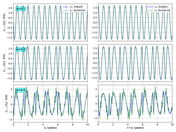
Figure 9: We overlay $s_{+,\times}(t)$ plots for an equal mass binary with different eccentricities that arise from our fully analytic post-circular approximation and the earlier described semi-analytic apporach. The binary parameters are the same as in Figure 5 with $P_{b}=1.5$ yrs at $t_{E}=0$ and the post-circular approximation includes all terms accurate up to $\mathcal{O}(e_{t}^{8})$. We observe that the quality of the post-circular approximation degrades as the eccentricity increases, as expected.

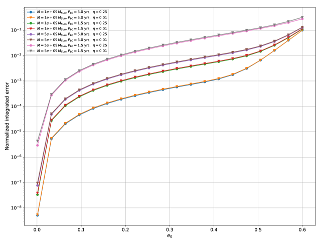
Figure 10: The normalized integrated error in the post-circular approximation as a function of the initial eccentricity for different combinations of $P_{b}$, $M$ and $\eta$. Rest of the binary parameters are identical to those used in Fig. 9 and the normalized integrated error is defined using Eq. (44). Clearly, the approximation gets progressively worse as we increase initial eccentricity values. In addition, the accuracy of the approximation decreases with shorter orbital periods and with higher masses. However, error is only weakly dependent on the mass ratio.

IV Summary and Discussions

The present work provides a computationally efficient way to compute pulsar timing residuals induced by GWs from isolated massive BH binaries inspiraling along general relativistic eccentric orbits. The use of an improvised version of the GW phasing approach, detailed in Damour2006,KonigsdorfferGopakumar2006,Refs. Ref. Damour et al. (2004); Königsdörffer and Gopakumar (2006), and the PN-accurate quasi-Keplerian parametrization allowed us to model binary BH orbits that inspiral due to the emission of quadrupolar GWs along 3PN-accurate eccentric orbits in an essentially analytic manner. This leads to analytic solutions for the mean motion $n$, mean anomaly $l$ and the periapsis angle $\gamma$ in terms of PN-accurate time eccentricity $e_{t}$ as well as system-dependent constants and initial conditions. This is augmented by using a computationally efficient way to obtain certain scaled temporal evolution for $e_{t}$ imposed by the quadrupolar order GW emission. These inputs allowed us to obtain the quadrupolar order temporally evolving GW polarization states, the associated $+/{\times}$ residuals and the resulting pulsar timing residuals $R(t)$ due to PN-accurate eccentric inspirals in a computationally inexpensive way. Additionally, we provided a fully analytic prescription to compute anaytic $+/{\times}$ residuals due to BH binaries moving in 3PN-accurate small eccentricity orbits. The excellent agreement between these two approaches provided a powerful check for our very involved semi-analytic approach, appropriate for arbitrary orbital eccentricities.

We have implemented our prescription to compute pulsar timing residuals induced by GWs from arbitrary eccentricity BH binaries, developed in Sec. II, as well as our fully analytic prescription to compute timing residuals for low-eccentricity binaries developed in Sec. III, in a C++ package called GWecc . We are working to integrate these codes into the popular PTA-relevant packages like TEMPO2 and Enterprise. This should allow us to constrain the presence of isolated eccentric BH binaries in the latest Parkes Pulsar Timing Array (PPTA) dataset Susobhanan et al. (prep). Further, efforts are on-going to tackle the IPTA DR2 and Nanograv 12.5 year datasets by employing the present prescription Cheeseboro et al. (prep). Clearly, it will be interesting to explore the effects of higher order GW radiation reaction effects in the equations for $\dot{n}$ and $\dot{e}_{t}$. It is reasonable to expect that such contributions will be more relevant for the pulsar contributions to $R(t)$ due to the lengthy temporal separation between the Earth and the Pulsar epochs and this is currently under investigation. Moreover, we are also pursuing detailed investigations on the implementation of certain Generalized Likelihood Ratio Test for the PTA detection of eccentric precessing BH binaries, influenced by Wang2015,Refs. Ref. Wang et al. (2015).

It turns out that the spin-orbit coupling can influence the nature of PTA signals from non-spinning massive BH binaries as this contribution enters the dynamics at the 1.5PN order. Therefore, we are extending the present approach by incorporating the spin effects, influenced by Mingarelli2012,ChenYang2018,Refs. Ref. Mingarelli et al. (2012); Chen and Zhang (2018). This effort relies on the availability of a Keplerian-type parametric solution for the dynamics of compact binaries that incorporates the effects of dominant order spin-orbit interactions Königsdörffer and Gopakumar (2005).

Appendix A Higher order PN corrections to $\gamma(t)$

This appendix details our approach to integrate 3PN-accurate expression for $d\gamma/dt$ which may be written symbolically as

$$\frac{d\gamma}{dt}=(k_{1}+k_{2}+k_{3})n\,,$$ (45)

Recall that we have tackled 1PN version of above equation, namely $d\gamma/dt=k_{1}\,n$ in subsection II.3. This appendix extends such a solution while incorporating 2PN and 3PN contributions to the rate of periapsis advance. The fact that this rate is independent of $\gamma$ allows us to express our Eq. (45) as

$$\frac{d\gamma_{j}}{dt}=k_{j}n\,,$$ (46)

where

$$\gamma=\sum_{j=1}^{\infty}\gamma_{j}\,.$$ (47)

At the 2PN order, we have Königsdörffer and Gopakumar (2006)

$$k_{2}=\left(\frac{GMn}{c^{3}}\right)^{4/3}\frac{\left((51-26\eta)e_{t}^{2}-28\eta+78\right)}{4\left(1-e_{t}^{2}\right)^{2}}\,.$$ (48)

This leads to

$$\frac{d\gamma_{2}}{dt}=\frac{1}{4}\left(\frac{GMn}{c^{3}}\right)^{4/3}n\frac{\left((51-26\eta)e_{t}^{2}-28\eta+78\right)}{\left(1-e_{t}^{2}\right)^{2}}\,.$$ (49)

Introducing $\tau$ variable with the help of Eqs. (19), (20b) and (21) allow us to write

$$\frac{d\gamma_{2}}{d\tau}=-\beta_{2}\frac{\left(1-e_{t}^{2}\right)^{\frac{3}{2}}}{e_{t}^{\frac{42}{19}}}\frac{\left((51-26\eta)e_{t}^{2}-28\eta+78\right)}{\left(304+121e_{t}^{2}\right)^{\frac{3045}{2299}}}\,,$$ (50)

where

$$\beta_{2}=\frac{15}{4}\left(\frac{GM_{\text{ch}}n_{0}}{c^{3}}\right)^{-5/3}\left(\frac{GMn_{0}}{c^{3}}\right)^{4/3}\frac{\sqrt{1-e_{t0}^{2}}}{e_{t0}^{6/19}\left(121e_{t0}^{2}+304\right)^{435/2299}}\,.$$ (51)

We now introduce $\bar{\gamma}_{2}=\Gamma_{20}-\frac{\gamma_{2}}{\beta_{2}}$, where $\Gamma_{20}$ is a constant. The above equation then becomes

$$\frac{d\bar{\gamma}_{2}}{d\tau}=\frac{\left(1-e_{t}^{2}\right)^{\frac{3}{2}}}{e_{t}^{\frac{42}{19}}}\frac{\left((51-26\eta)e_{t}^{2}-28\eta+78\right)}{\left(304+121e_{t}^{2}\right)^{\frac{3045}{2299}}}\,.$$ (52)

We define ${\gamma}_{2}$ such that $\gamma_{2}(\tau_{0})=0$. This allows us to fix $\Gamma_{20}$ to be $\Gamma_{20}=\bar{\gamma}_{2}(\tau_{0})$. We move on to obtain $d\bar{\gamma}_{2}/de_{t}$ by dividing Eq. (52) by Eq. (21), which gives us

$$\frac{d\bar{\gamma}_{2}}{de_{t}}=\frac{e_{t}^{2}(51-26\eta)-28\eta+78}{e_{t}^{13/19}\left(121e_{t}^{2}+304\right)^{\frac{1864}{2299}}}\,.$$ (53)

This can be integrated to obtain

$$\bar{\gamma}_{2}(e_{t})=\frac{e_{t}^{6/19}}{336}\left(4\left(121e_{t}^{2}+304\right)^{\frac{435}{2299}}(51-26\eta)+3\times 2^{\frac{1740}{2299}}19^{\frac{435}{2299}}(2\eta+23)\,_{2}\text{F}_{1}\left(\frac{3}{19},\frac{1864}{2299};\frac{22}{19};\frac{-121e_{t}^{2}}{304}\right)\right)\,.$$ (54)

Few comments are in order at this point. It should be obvious that we are splitting the GW emission-induced temporal evolution for $\gamma$ in parts. This is mainly because we assume that the GW emission is fully prescribed by Eqs. (17). And, it explains why we divided $d\bar{\gamma}_{1}/d\tau$ and $d\bar{\gamma}_{2}/d\tau$ equations the same equation, namely Eq. (21) for $de_{t}/d\tau$. In other words, the above split and our division of the resulting equations by Eq. (21) is rather inconsistent if there are higher order contributions to GW emission.

With the help of these considerations, we move on to write 3PN contributions to $d\gamma/dt$ as $d\gamma_{3}/dt=k_{3}\,n$ where

$$k_{3} =\left(\frac{GMn}{c^{3}}\right)^{2}\frac{1}{128(1-e_{t}^{2})^{3}}\left(18240-25376\eta+492\pi^{2}\eta+896\eta^{2}+(28128-27840\eta+123\pi^{2}\eta+5120\eta^{2})e_{t}^{2}\vphantom{\sqrt{1-e_{t}^{2}}}\right.$$

$$\quad\left.+(2496-1760\eta+1040\eta^{2})e_{t}^{4}+\left(1920-768\eta+(3840-1536\eta)e_{t}^{2}\right)\sqrt{1-e_{t}^{2}}\right)\,.$$ (55)

Following the steps that we pursued at the 2PN order lead us to

$$\frac{d\bar{\gamma}_{3}}{de_{t}} =\frac{1}{e_{t}^{\frac{25}{19}}\left(121e_{t}^{2}+304\right)^{\frac{2734}{2299}}}\left(18240-25376\eta+492\pi^{2}\eta+896\eta^{2}+(28128-27840\eta+123\pi^{2}\eta+5120\eta^{2})e_{t}^{2}\vphantom{\sqrt{1-e_{t}^{2}}}\right.$$

$$\quad\left.+(2496-1760\eta+1040\eta^{2})e_{t}^{4}+\left(1920-768\eta+(3840-1536\eta)e_{t}^{2}\right)\sqrt{1-e_{t}^{2}}\right)\,,$$ (56)

where we have defined $\bar{\gamma}_{3}=\Gamma_{30}-\frac{\gamma_{3}}{\beta_{3}}$, $\Gamma_{30}=\bar{\gamma}_{3}(\tau_{0})$. Further, the coefficient $\beta_{3}$ is given by

$$\beta_{3}=\frac{15}{128}\left(\frac{GM_{\text{ch}}n_{0}}{c^{3}}\right)^{-5/3}\left(\frac{GMn_{0}}{c^{3}}\right)^{2}\frac{e_{t0}^{6/19}\left(121e_{t0}^{2}+304\right){}^{435/2299}}{\sqrt{1-e_{t0}^{2}}}\;.$$ (57)

The equation for $\bar{\gamma}_{3}$ can be solved to get

$$\bar{\gamma}_{3}(e_{t})= -\frac{2957312\sqrt{1-e_{t}^{2}}(2\eta-5)\,\text{F}_{1}^{\text{A}}\left(\frac{-3}{19};\frac{-1}{2},\frac{2734}{2299};\frac{16}{19};e_{t}^{2},\frac{-121e_{t}^{2}}{304}\right)}{e_{t}^{6/19}\left(121e_{t}^{2}+304\right)^{\frac{2734}{2299}}}$$

$$\qquad\times\Bigg{[}e_{t}^{2}\left(1444\,\text{F}_{1}^{\text{A}}\left(\frac{16}{19};\frac{1}{2},\frac{2734}{2299};\frac{35}{19};e_{t}^{2},\frac{-121e_{t}^{2}}{304}\right)+1367\,\text{F}_{1}^{\text{A}}\left(\frac{16}{19};\frac{-1}{2},\frac{5033}{2299};\frac{35}{19};e_{t}^{2},\frac{-121e_{t}^{2}}{304}\right)\right)$$

$$\qquad\qquad-2432\,\text{F}_{1}^{\text{A}}\left(\frac{-3}{19};\frac{-1}{2},\frac{2734}{2299};\frac{16}{19};e_{t}^{2},\frac{-121e_{t}^{2}}{304}\right)\Bigg{]}^{-1}$$

$$+\frac{2425920e_{t}^{32/19}\sqrt{1-e_{t}^{2}}(2\eta-5)\,\text{F}_{1}^{\text{A}}\left(\frac{16}{19};\frac{-1}{2},\frac{2734}{2299};\frac{35}{19};e_{t}^{2},\frac{-121e_{t}^{2}}{304}\right)}{\left(121e_{t}^{2}+304\right)^{2734/2299}}$$

$$\qquad\times\Bigg{[}e_{t}^{2}\left(1444\,\text{F}_{1}^{\text{A}}\left(\frac{35}{19};\frac{1}{2},\frac{2734}{2299};\frac{54}{19};e_{t}^{2},\frac{-121e_{t}^{2}}{304}\right)+1367\,\text{F}_{1}^{\text{A}}\left(\frac{35}{19};\frac{-1}{2},\frac{5033}{2299};\frac{54}{19};e_{t}^{2},\frac{-121e_{t}^{2}}{304}\right)\right)$$

$$\qquad\qquad-5320\,\text{F}_{1}^{\text{A}}\left(\frac{16}{19};\frac{-1}{2},\frac{2734}{2299};\frac{35}{19};e_{t}^{2},\frac{-121e_{t}^{2}}{304}\right)\Bigg{]}^{-1}$$

$$+\frac{1}{53760\times 2^{1740/2299}19^{435/2299}e_{t}^{6/19}}$$

$$\qquad\times\Bigg{[}105e_{t}^{2}\left(5120\eta^{2}+3\left(41\pi^{2}-9280\right)\eta+28128\right)\,_{2}\text{F}_{1}\left(\frac{16}{19},\frac{2734}{2299};\frac{35}{19};\frac{-121e_{t}^{2}}{304}\right)$$

$$\qquad\qquad-2240\left(224\eta^{2}+\left(123\pi^{2}-6344\right)\eta+4560\right)\,_{2}\text{F}_{1}\left(\frac{-3}{19},\frac{2734}{2299};\frac{16}{19};\frac{-121e_{t}^{2}}{304}\right)$$

$$\qquad\qquad+768e_{t}^{4}\left(65\eta^{2}-110\eta+156\right)\,_{2}\text{F}_{1}\left(\frac{2734}{2299},\frac{35}{19};\frac{54}{19};\frac{-121e_{t}^{2}}{304}\right)\Bigg{]}\,.$$ (58)

Let us note again that we write

$$\gamma(e_{t})=\gamma_{0}-\beta_{1}\left(\bar{\gamma}_{1}(e_{t})-\bar{\gamma}_{1}(e_{t0})\right)-\beta_{2}\left(\bar{\gamma}_{2}(e_{t})-\bar{\gamma}_{2}(e_{t0})\right)-\beta_{3}\left(\bar{\gamma}_{3}(e_{t})-\bar{\gamma}_{3}(e_{t0})\right)\,.$$ (59)

as we strictly assume that the GW emission is fully characterised by our quadrupolar order equations.

Appendix B Reactive Evolution of Circular Orbits

This appendix lists the circular limit of GW phasing equations, detailed in Sec. II.3. A careful treatment is required as $\kappa\rightarrow 0$ for circular orbits. However, we may obtain $e_{t}\rightarrow 0$ limit of Eqs. (17) and it reads

$$\frac{dn}{dt} =\frac{96}{5}\left(\frac{GM_{\text{ch}}n}{c^{3}}\right)^{\frac{5}{3}}n^{2}\,,$$ (60a)

$$\frac{de_{t}}{dt} =0\,,$$ (60b)

$$\frac{dl}{dt} =n\,,$$ (60c)

$$\frac{d\gamma}{dt} =3\left(\frac{GMn}{c^{3}}\right)^{2/3}n+\frac{(78-28\eta)}{4}\left(\frac{GMn}{c^{3}}\right)^{4/3}n+\frac{\left(896\eta^{2}+492\pi^{2}\eta-26144\eta+20160\right)}{128}\left(\frac{GMn}{c^{3}}\right)^{2}n\,,$$ (60d)

where we have included the 2PN and 3PN contributions to $d\gamma/dt$, using the circular limits of Eqs. (48) and (55). Since the periapsis is not well-defined for a circular orbit, it is advisable to define the angular variable $\lambda=l+\gamma$ and the sidereal orbital frequency $n_{s}=(1+k)n$. It is straightforward to see that, in terms of $\lambda$ and $n_{s}$, the orbital evolution can be written as

$$\frac{dn_{s}}{dt} =\frac{96}{5}\left(\frac{GM_{\text{ch}}n_{s}}{c^{3}}\right)^{\frac{5}{3}}n_{s}^{2}\,,$$ (61a)

$$\frac{d\lambda}{dt} =n_{s}\,,$$ (61b)

where we have restricted the reactive evolution to the leading order in the PN expansion.

These equations lead to the following analytic expressions for $n_{s}(t)$ and $\lambda(t)$

$$n_{s}(t) =\frac{n_{s0}}{\left(1-\frac{256}{5}\left(\frac{GM_{\text{ch}}n_{s0}}{c^{3}}\right)^{\frac{5}{3}}n_{s0}(t-t_{0})\right)^{3/8}}\,,$$ (62a)

$$\lambda(t) =\lambda_{0}+\frac{1}{32}\left(\frac{GM_{\text{ch}}n_{s0}}{c^{3}}\right)^{-\frac{5}{3}}\left(1-\left(\frac{n_{s0}}{n_{s}}\right)^{5/3}\right)\,,$$ (62b)

where $n_{s0}$ and $\lambda_{0}$ are the values of these variables at some initial epoch $t=t_{0}$. The orbital eccentricity does not vary in time and its value is chosen to be zero.

The GW emission-induced merger time is obtained by demanding that $n\rightarrow\infty$ and this allows us to write

$$t_{\text{merg}}=t_{0}+\frac{5}{256n_{0}}\left(\frac{GM_{\text{ch}}n_{0}}{c^{3}}\right)^{-\frac{5}{3}}\,.$$ (63)

We have verified that our eccentric version of the merger time, given by Eq. (24), reduces to Eq. (63) in the circular limit.

References

- Kelley et al. (2017) L. Z. Kelley, L. Blecha, L. Hernquist, A. Sesana, and S. R. Taylor, Monthly Notices of the Royal Astronomical Society 471, 4508 (2017), http://oup.prod.sis.lan/mnras/article-pdf/471/4/4508/19609079/stx1638.pdf .
- The LIGO Scientific Collaboration and the Virgo Collaboration (2018) The LIGO Scientific Collaboration and the Virgo Collaboration, arXiv e-prints , arXiv:1811.12907 (2018), arXiv:1811.12907 [astro-ph.HE] .
- Foster and Backer (1990) R. S. Foster and D. C. Backer, Astrophys. J. 361, 300 (1990).
- Lommen (2015) A. N. Lommen, Reports on Progress in Physics 78, 124901 (2015).
- Detweiler (1979) S. Detweiler, Astrophys. J. 234, 1100 (1979).
- Hobbs (2013) G. Hobbs, Classical and Quantum Gravity 30, 224007 (2013), arXiv:1307.2629 [astro-ph.IM] .
- Kramer and Champion (2013) M. Kramer and D. J. Champion, Classical and Quantum Gravity 30, 224009 (2013).
- McLaughlin (2013) M. A. McLaughlin, Classical and Quantum Gravity 30, 224008 (2013), arXiv:1310.0758 [astro-ph.IM] .
- Brazier et al. (2019) A. Brazier, S. Chatterjee, T. Cohen, J. M. Cordes, M. E. DeCesar, P. B. Demorest, J. S. Hazboun, M. T. Lam, R. S. Lynch, M. A. McLaughlin, S. M. Ransom, X. Siemens, S. R. Taylor, and S. J. Vigeland , arXiv e-prints , arXiv:1908.05356 (2019), arXiv:1908.05356 [astro-ph.IM] .
- Joshi et al. (2018) B. C. Joshi, P. Arumugasamy, M. Bagchi, D. Bandyopadhyay, A. Basu, N. Dhanda Batra, S. Bethapudi, A. Choudhary, K. De, L. Dey, A. Gopakumar, Y. Gupta, M. A. Krishnakumar, Y. Maan, P. K. Manoharan, A. Naidu, R. Nandi, D. Pathak, M. Surnis, and A. Susobhanan, Journal of Astrophysics and Astronomy 39, 51 (2018).
- Bailes et al. (2018) M. Bailes, E. Barr, N. D. R. Bhat, J. Brink, S. Buchner, M. Burgay, F. Camilo, D. J. Champion, J. Hessels, G. H. Janssen, A. Jameson, S. Johnston, A. Karastergiou, R. Karuppusamy, V. Kaspi, M. J. Keith, M. Kramer, M. A. McLaughlin, K. Moodley, S. Oslowski, A. Possenti, S. M. Ransom, F. A. Rasio, J. Sievers, M. Serylak, B. W. Stappers, I. H. Stairs, G. Theureau, W. van Straten, P. Weltevrede, and N. Wex, arXiv e-prints , arXiv:1803.07424 (2018), arXiv:1803.07424 [astro-ph.IM] .
- Lee (2016) K. J. Lee, “Prospects of Gravitational Wave Detection Using Pulsar Timing Array for Chinese Future Telescopes,” in Frontiers in Radio Astronomy and FAST Early Sciences Symposium 2015, Astronomical Society of the Pacific Conference Series, Vol. 502, edited by L. Qain and D. Li (2016) p. 19.
- Hobbs et al. (2010) G. Hobbs, A. Archibald, Z. Arzoumanian, D. Backer, M. Bailes, N. D. R. Bhat, M. Burgay, S. Burke-Spolaor, D. Champion, I. Cognard, W. Coles, J. Cordes, P. Demorest, G. Desvignes, R. D. Ferdman, L. Finn, P. Freire, M. Gonzalez, J. Hessels, A. Hotan, G. Janssen, F. Jenet, A. Jessner, C. Jordan, V. Kaspi, M. Kramer, V. Kondratiev, J. Lazio, K. Lazaridis, K. J. Lee, Y. Levin, A. Lommen, D. Lorimer, R. Lynch, A. Lyne, R. Manchester, M. McLaughlin, D. Nice, S. Oslowski, M. Pilia, A. Possenti, M. Purver, S. Ransom, J. Reynolds, S. Sanidas, J. Sarkissian, A. Sesana, R. Shannon, X. Siemens, I. Stairs, B. Stappers, D. Stinebring, G. Theureau, R. van Haasteren, W. van Straten, J. P. W. Verbiest, D. R. B. Yardley, and X. P. You, Classical and Quantum Gravity 27, 084013 (2010), arXiv:0911.5206 [astro-ph.SR] .
- Verbiest et al. (2016) J. P. W. Verbiest, L. Lentati, G. Hobbs, R. van Haasteren, P. B. Demorest, G. H. Janssen, J.-B. Wang, G. Desvignes, R. N. Caballero, M. J. Keith, D. J. Champion, Z. Arzoumanian, S. Babak, C. G. Bassa, N. D. R. Bhat, A. Brazier, P. Brem, M. Burgay, S. Burke-Spolaor, S. J. Chamberlin, S. Chatterjee, B. Christy, I. Cognard, J. M. Cordes, S. Dai, T. Dolch, J. A. Ellis, R. D. Ferdman, E. Fonseca, J. R. Gair, N. E. Garver-Daniels, P. Gentile, M. E. Gonzalez, E. Graikou, L. Guillemot, J. W. T. Hessels, G. Jones, R. Karuppusamy, M. Kerr, M. Kramer, M. T. Lam, P. D. Lasky, A. Lassus, P. Lazarus, T. J. W. Lazio, K. J. Lee, L. Levin, K. Liu, R. S. Lynch, A. G. Lyne, J. Mckee, M. A. McLaughlin, S. T. McWilliams, D. R. Madison, R. N. Manchester, C. M. F. Mingarelli, D. J. Nice, S. Osłowski, N. T. Palliyaguru, T. T. Pennucci, B. B. P. Perera, D. Perrodin, A. Possenti, A. Petiteau, S. M. Ransom, D. Reardon, P. A. Rosado, S. A. Sanidas, A. Sesana, G. Shaifullah, R. M. Shannon, X. Siemens, J. Simon, R. Smits, R. Spiewak, I. H. Stairs, B. W. Stappers, D. R. Stinebring, K. Stovall, J. K. Swiggum, S. R. Taylor, G. Theureau, C. Tiburzi, L. Toomey, M. Vallisneri, W. van Straten, A. Vecchio, Y. Wang, L. Wen, X. P. You, W. W. Zhu, and X.-J. Zhu, Monthly Notices of the Royal Astronomical Society 458, 1267 (2016), arXiv:1602.03640 [astro-ph.IM] .
- Perera et al. (2019) B. B. P. Perera, M. E. DeCesar, P. B. Demorest, M. Kerr, L. Lentati, D. J. Nice, S. Oslowski, S. M. Ransom, M. J. Keith, Z. Arzoumanian, M. Bailes, P. T. Baker, C. G. Bassa, N. D. R. Bhat, A. Brazier, M. Burgay, S. Burke-Spolaor, R. N. Caballero, D. J. Champion, S. Chatterjee, S. Chen, I. Cognard, J. M. Cordes, K. Crowter, S. Dai, G. Desvignes, T. Dolch, R. D. Ferdman, E. C. Ferrara, E. Fonseca, J. M. Goldstein, E. Graikou, L. Guillemot, J. S. Hazboun, G. Hobbs, H. Hu, K. Islo, G. H. Janssen, R. Karuppusamy, M. Kramer, M. T. Lam, K. J. Lee, K. Liu, J. Luo, A. G. Lyne, R. N. Manchester, J. W. McKee, M. A. McLaughlin, C. M. F. Mingarelli, A. P. Parthasarathy, T. T. Pennucci, D. Perrodin, A. Possenti, D. J. Reardon, C. J. Russell, S. A. Sanidas, A. Sesana, G. Shaifullah, R. M. Shannon, X. Siemens, J. Simon, R. Spiewak, I. H. Stairs, B. W. Stappers, J. K. Swiggum, S. R. Taylor, G. Theureau, C. Tiburzi, M. Vallisneri, A. Vecchio, J. B. Wang, S. B. Zhang, L. Zhang, W. W. Zhu, and X. J. Zhu, arXiv e-prints , arXiv:1909.04534 (2019), arXiv:1909.04534 [astro-ph.HE] .
- Hobbs and Dai (2017) G. Hobbs and S. Dai, arXiv e-prints , arXiv:1707.01615 (2017), arXiv:1707.01615 [astro-ph.IM] .
- Burke-Spolaor et al. (2019) S. Burke-Spolaor, S. R. Taylor, M. Charisi, T. Dolch, J. S. Hazboun, A. M. Holgado, L. Z. Kelley, T. J. W. Lazio, D. R. Madison, N. McMann, C. M. F. Mingarelli, A. Rasskazov, X. Siemens, J. J. Simon, and T. L. Smith, Astronomy and Astrophysics Reviews 27, 5 (2019), arXiv:1811.08826 [astro-ph.HE] .
- Rosado et al. (2015) P. A. Rosado, A. Sesana, and J. Gair, Monthly Notices of the Royal Astronomical Society 451, 2417 (2015), http://oup.prod.sis.lan/mnras/article-pdf/451/3/2417/4008151/stv1098.pdf .
- Kelley et al. (2018) L. Z. Kelley, L. Blecha, L. Hernquist, A. Sesana, and S. R. Taylor, Monthly Notices of the Royal Astronomical Society 477, 964 (2018), arXiv:1711.00075 [astro-ph.HE] .
- Arzoumanian et al. (2018) Z. Arzoumanian, P. T. Baker, A. Brazier, S. Burke-Spolaor, S. J. Chamberlin, S. Chatterjee, B. Christy, J. M. Cordes, N. J. Cornish, F. Crawford, H. Thankful Cromartie, K. Crowter, M. DeCesar, P. B. Demorest, T. Dolch, J. A. Ellis, R. D. Ferdman, E. Ferrara, W. M. Folkner, E. Fonseca, N. Garver-Daniels, P. A. Gentile, R. Haas, J. S. Hazboun, E. A. Huerta, K. Islo, G. Jones, M. L. Jones, D. L. Kaplan, V. M. Kaspi, M. T. Lam, T. J. W. Lazio, L. Levin, A. N. Lommen, D. R. Lorimer, J. Luo, R. S. Lynch, D. R. Madison, M. A. McLaughlin, S. T. McWilliams, C. M. F. Mingarelli, C. Ng, D. J. Nice, R. S. Park, T. T. Pennucci, N. S. Pol, S. M. Ransom, P. S. Ray, A. Rasskazov, X. Siemens, J. Simon, R. Spiewak, I. H. Stairs, D. R. Stinebring, K. Stovall, J. Swiggum, S. R. Taylor, M. Vallisneri, R. van Haasteren, S. Vigeland , W. W. Zhu, and NANOGrav Collaboration, Astrophys. J. 859, 47 (2018), arXiv:1801.02617 [astro-ph.HE] .
- Aggarwal et al. (2019) K. Aggarwal, Z. Arzoumanian, P. T. Baker, A. Brazier, M. R. Brinson, P. R. Brook, S. Burke-Spolaor, S. Chatterjee, J. M. Cordes, N. J. Cornish, F. Crawford, K. Crowter, H. T. Cromartie, M. DeCesar, P. B. Demorest, T. Dolch, J. A. Ellis, R. D. Ferdman, E. Ferrara, E. Fonseca, N. Garver-Daniels, P. Gentile, J. S. Hazboun, A. M. Holgado, E. A. Huerta, K. Islo, R. Jennings, G. Jones, M. L. Jones, A. R. Kaiser, D. L. Kaplan, L. Z. Kelley, J. S. Key, M. T. Lam, T. J. W. Lazio, L. Levin, D. R. Lorimer, J. Luo, R. S. Lynch, D. R. Madison, M. A. McLaughlin, S. T. McWilliams, C. M. F. Mingarelli, C. Ng, D. J. Nice, T. T. Pennucci, N. S. Pol, S. M. Ransom, P. S. Ray, X. Siemens, J. Simon, R. Spiewak, I. H. Stairs, D. R. Stinebring, K. Stovall, J. Swiggum, S. R. Taylor, J. E. Turner, M. Vallisneri, R. van Haasteren, S. J. Vigeland , C. A. Witt, W. W. Zhu, and (The NANOGrav Collaboration, Astrophys. J. 880, 116 (2019), arXiv:1812.11585 [astro-ph.GA] .
- Babak et al. (2015) S. Babak, A. Petiteau, A. Sesana, P. Brem, P. A. Rosado, S. R. Taylor, A. Lassus, J. W. T. Hessels, C. G. Bassa, M. Burgay, R. N. Caballero, D. J. Champion, I. Cognard, G. Desvignes, J. R. Gair, L. Guillemot, G. H. Janssen, R. Karuppusamy, M. Kramer, P. Lazarus, K. J. Lee, L. Lentati, K. Liu, C. M. F. Mingarelli, S. Osłowski, D. Perrodin, A. Possenti, M. B. Purver, S. Sanidas, R. Smits, B. Stappers, G. Theureau, C. Tiburzi, R. van Haasteren, A. Vecchio, and J. P. W. Verbiest, Monthly Notices of the Royal Astronomical Society 455, 1665 (2015), http://oup.prod.sis.lan/mnras/article-pdf/455/2/1665/18509657/stv2092.pdf .
- Lentati et al. (2015) L. Lentati, S. R. Taylor, C. M. F. Mingarelli, A. Sesana, S. A. Sanidas, A. Vecchio, R. N. Caballero, K. J. Lee, R. van Haasteren, S. Babak, C. G. Bassa, P. Brem, M. Burgay, D. J. Champion, I. Cognard, G. Desvignes, J. R. Gair, L. Guillemot, J. W. T. Hessels, G. H. Janssen, R. Karuppusamy, M. Kramer, A. Lassus, P. Lazarus, K. Liu, S. Osłowski, D. Perrodin, A. Petiteau, A. Possenti, M. B. Purver, P. A. Rosado, R. Smits, B. Stappers, G. Theureau, C. Tiburzi, and J. P. W. Verbiest, Monthly Notices of the Royal Astronomical Society 453, 2576 (2015), arXiv:1504.03692 [astro-ph.CO] .
- Feng et al. (2019) Y. Feng, D. Li, Y.-R. Li, and J.-M. Wang, arXiv e-prints , arXiv:1907.03460 (2019), arXiv:1907.03460 [astro-ph.IM] .
- Porayko et al. (2018) N. K. Porayko, X. Zhu, Y. Levin, L. Hui, G. Hobbs, A. Grudskaya, K. Postnov, M. Bailes, N. D. R. Bhat, W. Coles, S. Dai, J. Dempsey, M. J. Keith, M. Kerr, M. Kramer, P. D. Lasky, R. N. Manchester, S. Osłowski, A. Parthasarathy, V. Ravi, D. J. Reardon, P. A. Rosado, C. J. Russell, R. M. Shannon, R. Spiewak, W. van Straten, L. Toomey, J. Wang, L. Wen, X. You, and PPTA Collaboration, Phys. Rev. D 98, 102002 (2018), arXiv:1810.03227 [astro-ph.CO] .
- Middleton et al. (2018) H. Middleton, S. Chen, W. Del Pozzo, A. Sesana, and A. Vecchio, Nature Communications 9, 573 (2018), arXiv:1707.00623 [astro-ph.GA] .
- Chen et al. (2019) S. Chen, A. Sesana, and C. J. Conselice, Monthly Notices of the Royal Astronomical Society 488, 401 (2019), arXiv:1810.04184 [astro-ph.GA] .
- Chen et al. (2017) S. Chen, H. Middleton, A. Sesana, W. Del Pozzo, and A. Vecchio, Monthly Notices of the Royal Astronomical Society 468, 404 (2017), arXiv:1612.02826 [astro-ph.HE] .
- Taylor et al. (2019) S. Taylor, S. Burke-Spolaor, P. T. Baker, M. Charisi, K. Islo, L. Z. Kelley, D. R. Madison, J. Simon, S. Vigeland, and Nanograv Collaboration, Bulletin of the AAS 51, 336 (2019), arXiv:1903.08183 [astro-ph.GA] .
- Taylor et al. (2017) S. R. Taylor, J. Simon, and L. Sampson, Phys. Rev. Lett. 118, 181102 (2017), arXiv:1612.02817 [astro-ph.GA] .
- Armitage and Natarajan (2005) P. J. Armitage and P. Natarajan, Astrophys. J. 634, 921 (2005), arXiv:astro-ph/0508493 [astro-ph] .
- Cuadra et al. (2009) J. Cuadra, P. J. Armitage, R. D. Alexander, and M. C. Begelman, Monthly Notices of the Royal Astronomical Society 393, 1423 (2009), https://academic.oup.com/mnras/article-pdf/393/4/1423/3254986/mnras0393-1423.pdf .
- Berentzen et al. (2009) I. Berentzen, M. Preto, P. Berczik, D. Merritt, and R. Spurzem, Astrophys. J. 695, 455 (2009), arXiv:0812.2756 [astro-ph] .
- Khan et al. (2012) F. M. Khan, M. Preto, P. Berczik, I. Berentzen, A. Just, and R. Spurzem, Astrophys. J. 749, 147 (2012), arXiv:1202.2124 [astro-ph.CO] .
- Khan et al. (2013) F. M. Khan, K. Holley-Bockelmann, P. Berczik, and A. Just, Astrophys. J. 773, 100 (2013), arXiv:1302.1871 [astro-ph.GA] .
- Roedig and Sesana (2012) C. Roedig and A. Sesana, in Journal of Physics Conference Series, Journal of Physics Conference Series, Vol. 363 (2012) p. 012035, arXiv:1111.3742 [astro-ph.CO] .
- Edwards et al. (2006) R. T. Edwards, G. B. Hobbs, and R. N. Manchester, Monthly Notices of the Royal Astronomical Society 372, 1549 (2006), http://oup.prod.sis.lan/mnras/article-pdf/372/4/1549/4012423/mnras0372-1549.pdf .
- Hobbs et al. (2006) G. B. Hobbs, R. T. Edwards, and R. N. Manchester, Monthly Notices of the Royal Astronomical Society 369, 655 (2006), astro-ph/0603381 .
- Ellis et al. (2017) J. A. Ellis, S. R. Taylor, P. T. Baker, and M. Vallisneri, “nanograv/enterprise,” (2017).
- Blanchet (2014) L. Blanchet, Living Reviews in Relativity 17, 2 (2014), arXiv:1310.1528 [gr-qc] .
- Memmesheimer et al. (2004) R.-M. Memmesheimer, A. Gopakumar, and G. Schäfer, Phys. Rev. D 70, 104011 (2004).
- Damour et al. (2004) T. Damour, A. Gopakumar, and B. R. Iyer, Phys. Rev. D 70, 064028 (2004).
- Königsdörffer and Gopakumar (2006) C. Königsdörffer and A. Gopakumar, Phys. Rev. D 73, 124012 (2006).
- Moore et al. (2018) B. Moore, T. Robson, N. Loutrel, and N. Yunes, Classical and Quantum Gravity 35, 235006 (2018).
- Boetzel et al. (2017) Y. Boetzel, A. Susobhanan, A. Gopakumar, A. Klein, and P. Jetzer, Phys. Rev. D 96, 044011 (2017).
- Jenet et al. (2004) F. A. Jenet, A. Lommen, S. L. Larson, and L. Wen, The Astrophysical Journal 606, 799 (2004).
- Taylor et al. (2016) S. R. Taylor, E. A. Huerta, J. R. Gair, and S. T. McWilliams, The Astrophysical Journal 817, 70 (2016).
- Book and Flanagan (2011) L. G. Book and É. Flanagan, Phys. Rev. D 83, 024024 (2011), arXiv:1009.4192 [astro-ph.CO] .
- Wahlquist (1987) H. Wahlquist, General Relativity and Gravitation 19, 1101 (1987).
- Lee et al. (2011) K. J. Lee, N. Wex, M. Kramer, B. W. Stappers, C. G. Bassa, G. H. Janssen, R. Karuppusamy, and R. Smits, Monthly Notices of the Royal Astronomical Society 414, 3251 (2011), http://oup.prod.sis.lan/mnras/article-pdf/414/4/3251/18708099/mnras0414-3251.pdf .
- Damour and Deruelle (1985) T. Damour and N. Deruelle, Ann. Inst. Henri Poincaré Phys. Théor., Vol. 43, No. 1, p. 107 - 132 43, 107 (1985).
- Tanay et al. (2016) S. Tanay, M. Haney, and A. Gopakumar, Phys. Rev. D 93, 064031 (2016), arXiv:1602.03081 [gr-qc] .
- Tiwari et al. (2019) S. Tiwari, A. Gopakumar, M. Haney, and P. Hemantakumar, Phys. Rev. D 99, 124008 (2019), arXiv:1905.07956 [gr-qc] .
- Mikkola (1987) S. Mikkola, Celest. Mech. 40, 329 (1987).
- Colavecchia et al. (2001) F. Colavecchia, G. Gasaneo, and J. Miraglia, Computer Physics Communications 138, 29 (2001).
- Królak et al. (1995) A. Królak, K. D. Kokkotas, and G. Schäfer, Phys. Rev. D 52, 2089 (1995).
- Tessmer and Gopakumar (2007) M. Tessmer and A. Gopakumar, Monthly Notices of the Royal Astronomical Society 374, 721 (2007), gr-qc/0610139 .
- Zwillinger (1992) D. Zwillinger, The Handbook of Integration, 1st ed. (Jones and Bartlett, 1992).
- Reardon et al. (2016) D. J. Reardon, G. Hobbs, W. Coles, Y. Levin, M. J. Keith, M. Bailes, N. D. R. Bhat, S. Burke-Spolaor, S. Dai, M. Kerr, P. D. Lasky, R. N. Manchester, S. Osłowski, V. Ravi, R. M. Shannon, W. van Straten, L. Toomey, J. Wang, L. Wen, X. P. You, and X. J. Zhu, Monthly Notices of the Royal Astronomical Society 455, 1751 (2016), arXiv:1510.04434 [astro-ph.HE] .
- Colwell (1993) P. Colwell, Solving Kepler’s equation over three centuries (Willmann-Bell, 1993).
- Peters and Mathews (1963) P. C. Peters and J. Mathews, Phys. Rev. 131, 435 (1963).
- Moreno-Garrido et al. (1995) C. Moreno-Garrido, E. Mediavilla, and J. Buitrago, Monthly Notices of the Royal Astronomical Society 274, 115 (1995).
- Seto (2001) N. Seto, Phys. Rev. Lett. 87, 251101 (2001).
- Barack and Cutler (2004) L. Barack and C. Cutler, Phys. Rev. D 69, 082005 (2004), gr-qc/0310125 .
- Watson (1966) G. N. Watson, A Treatise on the Theory of Bessel Functions, 2nd ed. (Cambridge University Press, 1966).
- Note (1) GWecc, together with a Python wrapper, are available at https://github.com/abhisrkckl/GWecc.
- Susobhanan et al. (prep) A. Susobhanan, X. J. Zhu, G. Hobbs, A. Gopakumar, and et al., (In prep.).
- Cheeseboro et al. (prep) B. Cheeseboro, L. Dey, A. Susobhanan, S. Burke-Spolaor, A. Gopakumar, and et al., (In prep.).
- Wang et al. (2015) Y. Wang, S. D. Mohanty, and F. A. Jenet, Astrophys. J. 815, 125 (2015), arXiv:1506.01526 [astro-ph.IM] .
- Mingarelli et al. (2012) C. M. F. Mingarelli, K. Grover, T. Sidery, R. J. E. Smith, and A. Vecchio, Phys. Rev. Lett. 109, 081104 (2012).
- Chen and Zhang (2018) J.-W. Chen and Y. Zhang, Monthly Notices of the Royal Astronomical Society 481, 2249 (2018), http://oup.prod.sis.lan/mnras/article-pdf/481/2/2249/25791934/sty2268.pdf .
- Königsdörffer and Gopakumar (2005) C. Königsdörffer and A. Gopakumar, Phys. Rev. D 71, 024039 (2005).