Abstract

It is a challenging issue to analyze complex dynamics from observed and simulated data. An advantage of extracting dynamic behaviors from data is that this approach enables the investigation of nonlinear phenomena whose mathematical models are unavailable. The purpose of this present work is to extract information about transition phenomena (e.g., mean exit time and escape probability), from data of stochastic differential equations with non-Gaussian Lévy noise. As a tool in describing dynamical systems, the Koopman semigroup transforms a nonlinear system into a linear system, but at the cost of elevating a finite dimensional problem into an infinite dimensional one. In spite of this, using the relation between the stochastic Koopman semigroup and the infinitesimal generator of a stochastic differential equation, we learn the mean exit time and escape probability from data. Specifically, we first obtain a finite dimensional approximation of the infinitesimal generator by an extended dynamic mode decomposition algorithm. Then we identify the drift coefficient, diffusion coefficient and anomalous diffusion coefficient for the stochastic differential equation. Finally, we compute the mean exit time and escape probability by finite difference discretization of the associated nonlocal partial differential equations. This approach is applicable in extracting transition information from data of stochastic differential equations with either (Gaussian) Brownian motion or (non-Gaussian) Lévy motion. We present one - and two-dimensional examples to demonstrate the effectiveness of our approach.

Key Words and Phrases: Transition phenomena, Koopman operator, nonlocal generator, Lévy motion, non-Gaussian noise, stochastic differential equations.

The transition behavior in stochastic dynamical systems is often quantified in terms of deterministic indexes (e.g., mean exit time, escape probability), leading to simple and effective prediction. However, the discovery of such indexes usually relies on a deep understanding and priori knowledge of the system, as well as extensive and time-consuming mathematical justification. Recent developments in data-driven computational approaches suggest alternative ways toward discovering deterministic indexes directly from data. It is intriguing to note that obtaining such deterministic indexes for stochastic dynamical systems accurately and efficiently is still a significant challenge. In this paper, we extract deterministic indexes from data of a stochastic dynamical system with Lévy noise, after identifying the system by adapting a method to learn the associated Koopman semigroup and its generator.

1 Introduction

Stochastic differential equations are widely used to model complex phenomena in climate dynamics, molecular dynamics, biophysical dynamics, and other engineering systems, under random fluctuations. Usually, we build a mathematical model for such a system based on available governing laws, and then analyze or simulate the model to gain insights about its nonlinear phenomena (e.g., transition phenomena [20]). However, sometimes it is difficult to build a model for a complex phenomenon due to lack of scientific understanding. At some other times, a mathematical model based on governing laws may be too complicated for analysis. Fortunately, with the development of observing techniques and computing power, there are a lot of valuable observation data when a model is unavailable, or simulated data when a model is too complicated yet computable. Therefore, it is desirable to discover dynamical quantities and gain insights about stochastic phenomena directly from these data sets.

Data-driven analysis of complex dynamic behavior has recently attracted increasing attention. Many authors have proposed various methods to analyze complex dynamic behaviors from data. These include, for example, stochastic parametrization [1], parameters estimation of stochastic differential equations using Gaussian process [2, 3], Sparse Identification of Nonlinear Dynamics [4, 5], Kramers-Moyal expansion [6], the Koopman operator analysis, for analyzing complex dynamic behaviors [7, 8, 9, 10, 11, 12], and transfer operators for analyzing stochastic dynamic behaviors [13, 14, 15, 16, 17, 18, 19], among others. However, most of these authors focused on deterministic dynamical systems, or stochastic dynamical systems with Gaussian noise.

In this present work, we devise a method to extract the mean exit time and escape probability from data, for a stochastic dynamical system with non-Gaussian stable Lévy noise. These two quantities provide insights about transition phenomena under the interaction of nonlinearity and uncertainty [20]. We first infer the generator for this non-Gaussian stochastic dynamical system, with help of the Koopman operator, which fortunately also deals with dynamical systems with noise. Then we identify the coefficients in this stochastic system, and finally we discretize nonlocal partial differential equations to obtain the mean exit time and escape probability. The main contribution of this present work is an algorithm to estimate the coefficient of the non-Gaussian Levy noise from dynamical data, and thus further enable to extract transition information from the same data.

The remainder of this paper is arranged as follows: In Section 2, we present the theoretical background, including the definition of Koopman operator and infinitesimal generator, and then the mean exit time and escape probability. In Section 3, we will introduce the adapted EDMD algorithm and the method of system identification. In Section 4, we will conduct numerical experiments, including stochastic differential equations with Brownian motion and Lévy motion, in one-dimensional and two-dimensional cases. We leave the discussion in the final section.

2 Theory

We recall the Koopman semigroup of operators and its generator in Section 2.1, and then introduce deterministic quantities, mean exit time and escape probability, for stochastic dynamics in Section 2.2.

2.1 The Koopman operator and the generator

Let $\mathcal{M}$ be the state space in $\mathbb{R}^{d}$. Consider a stochastic differential equation in $\mathcal{M}$

$$dX_{t}=b(X_{t})dt+\sigma_{1}(X_{t})dW_{t}+\sigma_{2}d\tilde{L}_{t}^{\alpha},$$ (2.1)

with the drift coefficient (or vector field) $b$ in $\mathbb{R}^{d}$, diffusion coefficient $d\times d$ diagonal matrix $\sigma_{1}$, $d-$dimensional Brownian motion $W_{t}$ and $d-$dimensional Lévy motion $\tilde{L}_{t}^{\alpha}$. The components of $\tilde{L}_{t}^{\alpha}$ are one-dimensional mutually independent and symmetric with the same triple $(0,0,\tilde{\nu})$ Lévy motion, where $\tilde{\nu}(dx)=C_{\alpha}I_{\{\|x\|<c\}}(x)\frac{dx}{|x|^{1+\alpha}}$ for $x\in\mathbb{R}\setminus\{0\}$. Here $c$ is a positive constant (usually we take $c=1$), $I$ is a indicator function and

$$C_{\alpha}=\frac{\alpha\Gamma(\frac{1+\alpha}{2})}{2^{1-\alpha}\pi^{\frac{1}{2}}\Gamma(1-\frac{\alpha}{2})}.$$

Moreover, the anomalous diffusion coefficient $\sigma_{2}$ is a constant $d\times d$ diagonal matrix. Since Lévy motion is symmetric, without loss of generality, we can set $\sigma_{2}\geq 0$. In this paper we assume that the stability index $\alpha$ is known. More details about Lévy motion are in Appendix.
The associated Koopman semigroup of operators $\{\mathcal{K}^{t}\}$ is defined as

$$(\mathcal{K}^{t}f)(x)=\mathbb{E}[f(\Phi^{t}(x,\omega))],$$ (2.2)

where $f:\mathbb{R}^{d}\rightarrow\mathbb{R}$ a real-valued measurable function, $\Phi^{t}(x,\omega)$ is the solution of (2.1) with initial value $x$ and $\mathbb{E}[\cdot]$ denotes the expected value. The infinitesimal generator $\mathcal{L}$ of this Koopman semigroup is the derivative of $\mathcal{K}^{t}$ at $t=0$.

$$\mathcal{L}f=\lim\limits_{t\to 0}\frac{1}{t}(\mathcal{K}^{t}f-f).$$ (2.3)

Thus, if $f\in Dom(\mathcal{L})$, the infinitesimal generator is a nonlocal partial differential operator

$$\mathcal{L}f =\sum_{i=1}^{d}b_{i}\frac{\partial{f}}{\partial{x_{i}}}+\frac{1}{2}\sum_{i=1}^{d}\sum_{j=1}^{d}a_{ij}\frac{\partial^{2}f}{\partial{x_{i}}\partial{x_{j}}}$$

$$+C_{\alpha}\sum_{i=1}^{d}\int_{\mathbb{R}\backslash\{0\}}[f(x_{i}+(\sigma_{2})_{ii}y_{i})-f(x_{i})]I_{\{\|y_{i}\|<c\}}(y_{i})\,\frac{dy_{i}}{|y_{i}|^{1+\alpha}},$$ (2.4)

where the coefficient $a=\sigma_{1}\mathbf{\sigma}_{1}^{\top}$ is sometimes also called diffusion coefficient. For more details see [24, 25].

When the Lévy motion is absent, the third term in this generator is absent (because Brownian motion has no jumps) and the generator becomes a local partial differential operator

$$\mathcal{L_{B}}f =\sum_{i=1}^{d}b_{i}\frac{\partial{f}}{\partial{x_{i}}}+\frac{1}{2}\sum_{i=1}^{d}\sum_{j=1}^{d}a_{ij}\frac{\partial^{2}f}{\partial{x_{i}}\partial{x_{j}}}.$$ (2.5)

2.2 Deterministic quantities for transition phenomena

We mainly discuss mean exit time and escape probability with non-Gaussian noise, as deterministic quantities that carry dynamical information for solution orbits of (2.1). In what follows, we assume that $D$ is a regular bounded open domain in $\mathbb{R}^{d}$.

Mean Exit Time

We first consider the mean exit time. Define the first exit time $\tau_{x}$ of a solution path starting at $x$ from domain $D$ as

$$\tau_{x}(\omega)=inf\{t\geq 0,X_{0}=x,X_{t}(\omega,x)\not\in D\}.$$ (2.6)

The mean exit time is then denoted by

$$u(x)=\mathbb{E}^{x}[\tau_{x}(\omega)],$$ (2.7)

for $x\in D$.
As usual, we assume that the drift coefficient and diffusion coefficient satisfy an appropriate local Lipschitz condition. Moreover, we assume that the generator operator of this system is uniformly elliptic. For more details, see [20, 21]. Under these conditions, the mean exit time $u(x)$, for a solution path starting at $x\in D$, satisfies the following nonlocal partial differential equation

$$\mathcal{L}u=-1,$$ (2.8)

with “an external” Dirichlet boundary condition

$$u\mid_{D^{c}}=0,$$ (2.9)

where $\mathcal{L}$ is the generator (2.1), and $D^{c}$ is the complement of the domain $D$ in $\mathbb{R}^{d}$.

Escape Probability

Here we just recall the escape probability for stochastic system with Lévy motion. Assume that $X_{t}(\omega)$ is the solution of (2.1). Now we consider the escape probability of $X_{t}(\omega)$. Define the first exit time

$$\tau_{D^{c}}(\omega)\triangleq\inf\{t>0:X_{t}(\omega)\in D^{c}\}.$$ (2.10)

We take a subset $U$ of $D^{c}$, and define the likelihood that $X_{t}(\omega)$ exits firstly from $D$ by landing in the target set $U$ as the escape probability from $D$ to $U$, denoted by $p(x)$. That is

$$p(x)=\mathbb{P}\{X_{\tau_{D^{c}}}(\omega)\in U\}.$$ (2.11)

Then the escape probability $p$, for the dynamical system driven by Lévy motion (2.1), from $D$ to $U$, is the solution of the following nonlocal partial differential equations with Balayage-Dirichlet external boundary conditions

$$\mathcal{L}p=0,$$

$$p\mid_{U}=1,$$

$$p\mid_{D^{c}\setminus U}=0,$$ (2.12)

where $\mathcal{L}$ is the generator (2.1).

For a system with only Brownian motion, the sample paths are continuous and thus can only exit domain $D$ by passing its boundary $\partial D$, or escape through a portion $U$ of the boundary. Therefore, the mean exit time $u$ satisfies

$$\mathcal{L_{B}}\;u=-1,\;\;\;u\mid_{\partial D}=0.$$ (2.13)

Moreover, the escape probability $p$, through a portion $U$ of the boundary, satisfies

$$\mathcal{L_{B}}\;p=0,$$

$$p\mid_{U}=1,$$

$$p\mid_{\partial D\setminus U}=0.$$ (2.14)

For more details see [20].

3 Numerical schemes

In this section, we will review briefly the extended dynamic mode decomposition in Section 3.1, and then identify system in Section 3.2. Finally, we will propose a algorithm for discovering transition phenomena from data in Section 3.3.

3.1 Extended Dynamic Mode Decomposition

In this subsection, we review breifly extended dynamic mode decomposition(EDMD), which can approximate Koopman operators. Of course, EDMD can also approximate Koopman eigenvalue, eigenfunction and mode tuples as described by [8], but we will not consider them here.

We adopt the notations from [8]. There are two prerequisites in the EDMD procedure:
(a) A data set of snapshot pairs, i.e., $\{(x_{m},y_{m})\}_{m=1}^{M}$ that we will organize as a pair of data sets,

$$X=[x_{1},x_{2},\ldots,x_{M}],$$

$$Y=[y_{1},y_{2},\ldots,y_{M}],$$ (3.1)

where $x_{i}\in\mathcal{M}$ and $y_{i}\in\mathcal{M}$ satisfy $y_{i}=\Phi^{t}(x_{i},\omega)$.
(b) Assume that $\mathcal{F}=L^{2}(\mathcal{M})$. A dictionary of observables $\mathcal{D}=\{\psi_{1},\psi_{2},\ldots,\psi_{N_{k}}\}$, where $\psi_{i}\in\mathcal{F}$, whose span we denote as $\mathcal{F}_{\mathcal{D}}\subset\mathcal{F}$; for the sake of simplicity, we also denote it by a vector-valued function $\Psi:\mathcal{M}\rightarrow\mathbb{C}^{1\times N_{K}}$ as follows

$$\Psi(x)=[\psi_{1}(x),\psi_{2}(x),\ldots,\psi_{N_{k}}(x)].$$ (3.2)

A function $f\in\mathcal{F}_{\mathcal{D}}$ can be written as $f=B^{\top}\Psi^{\top}$, where $B$ is a weight vector. Because $\mathcal{F}_{\mathcal{D}}$ is not an invariant subspace of $\mathcal{K}$, we obtain the follow relation with a residual term $r(x)$:

$$(\mathcal{K}^{\Delta t}f)(x) =\mathbb{E}[f\circ\Phi^{\Delta t}(x,\omega)]$$

$$=B^{\top}\mathbb{E}[\Psi^{\top}\circ\Phi^{\Delta t}(x,\omega)]+r(x)$$

$$=(KB)^{\top}\Psi^{\top}(x)+r(x).$$ (3.3)

Then we will minimize the residual term $r(x)$ to obtain the matrix $K=G^{+}A$, where $+$ denotes the pseudoinverse and

$$G=\frac{1}{M}\sum_{m=1}^{M}\Psi(x_{m})^{*}\Psi(x_{m}),$$ (3.4)

$$A=\frac{1}{M}\sum_{m=1}^{M}\Psi(x_{m})^{*}\Psi(y_{m}).$$ (3.5)

Here matrices $K,G,A\in\mathbb{C}^{N_{K}\times N_{K}}$.
Therefore, we have a matrix $K$ such that

$$(\mathcal{K}^{\Delta t}f)(x)\approx(KB)^{\top}\Psi^{\top},$$ (3.6)

where $\Delta t$ is small enough.
Using the definition for the generator $\mathcal{L}f=\lim\limits_{t\to 0}\frac{1}{t}(\mathcal{K}^{t}f-f)$, we can get a finite-dimensional approximation of generator $\mathcal{L}$ by finite-dimensional approximation $K$ of the stochastic Koopman operator $\mathcal{K}$. This approximated generator is denoted by $L$.

This approximated generator $L$ can not be directly used in solving partial differential equations for mean exit time and escape probability, as these two dynamical quantities satisfy special boundary conditions as in Section 2.2. So we next need to identify coefficients in the stochastic differential equation (2.1), and use these coefficients in discretizing partial differential equations to obtain mean exit time and escape probability.

3.2 System identification

In this subsection, we will state the method for identifying system parameters using generator operator. Assume that the drift coefficient and diffusion coefficients of a stochastic differential equation can be expanded by basis functions $\Psi(x)$. We assume that the diffusion coefficients $\sigma_{1}$ and $\sigma_{2}$ are diagonal matrices. Indeed, $\sigma_{1}$ does not need to be a diagonal matrix, but our method requires that $\sigma_{2}$ to be diagonal; See Remark 3.5.
Given the full-state observable

$$f_{1i}(x)=x_{i},i=1,2,\ldots,d,$$

where $x=(x_{1},x_{2},\ldots,x_{d})\in\mathbb{R}^{d}$.
With the aid of generator operator $\mathcal{L}$ and its finite-dimensional approximation $L$, described in previous section, it is possible to discover the governing equations. Assume that $B_{1i}\in\mathbb{R}^{N_{K}\times 1}$ is the vector such that $f_{1i}(x)=B_{1i}^{\top}\Psi(x)^{\top}$. We can express the drift coefficient in terms of the basis functions, i.e.,

$$(\mathcal{L}f_{1})(x)=b(x)\approx(LB_{1i})^{\top}\Psi(x)^{\top}.$$ (3.7)

Similarity, let $f_{2i}(x)=x_{i}^{2}$, we can get the diffusion coefficients by finding another matrix $B_{2i}\in\mathbb{R}^{N_{K}\times 1}$ such that $f_{2i}(x)=B_{2i}^{\top}\Psi(x)^{\top}$

$$(\mathcal{L}f_{2i})(x) =2b_{i}(x)x_{i}+a_{ii}(x)$$

$$+C_{\alpha}\int_{\mathbb{R}\backslash\{0\}}\frac{[(x_{i}+(\sigma_{2})_{ii}y_{i})^{2}-x_{i}^{2}]I_{\{\|y_{i}\|<c\}}(y_{i})}{|y_{i}|^{1+\alpha}}\,dy_{i}\approx(LB_{2i})^{\top}\Psi(x)^{\top},$$ (3.8)

Note that, in order to make sure the integral in (3.2) exists, we assume that the Lévy motion has bounded jump size with bound $c$ (a positive constant). Moreover, using the properties of odd functions, the integral term can be represented by

$$\int_{\mathbb{R}\backslash\{0\}}\frac{[(x_{i}+(\sigma_{2})_{ii}y_{i})^{2}-x_{i}^{2}]I_{\{\|y_{i}\|<c\}}(y_{i})}{|y_{i}|^{1+\alpha}}\,dy_{i}=(\sigma_{2})_{ii}^{2}\int_{\mathbb{R}\backslash\{0\}}\frac{y_{i}^{2}I_{\{\|y_{i}\|<c\}}(y_{i})}{|y_{i}|^{1+\alpha}}\,dy_{i}.$$ (3.9)

Therefore we can rewrite (3.2) as follows

$$(\mathcal{L}f_{2i})(x) =2b_{i}(x)x_{i}+a_{ii}(x)$$

$$+(\sigma_{2})_{ii}^{2}C_{\alpha}\int_{\mathbb{R}\backslash\{0\}}\frac{y_{i}^{2}}{|y_{i}|^{1+\alpha}}I_{\{\|y_{i}\|<c\}}(y_{i})\,dy_{i}.$$ (3.10)

Note that there are two unknown coefficients in (3.2), i.e., diffusion coefficient $a$ and anomalous diffusion coefficient $\sigma_{2}$. In general, one equation can not determine two unknown coefficients. However, we will explain this can actually be done in our particular setting. We present this for a scalar system in the following proposition.

Proposition 3.1

Consider a scalar stochastic differential equation

$$dX_{t}=b(X_{t})dt+\sigma_{1}(X_{t})dW_{t}+\sigma_{2}d\tilde{L}_{t}^{\alpha},$$ (3.11)

where the drift coefficient $b(x)=\sum_{i=0}^{p_{1}}\xi_{i}x^{i}$, diffusion coefficient $\sigma_{1}(x)=\sum_{j=0}^{p_{2}}\eta_{j}x^{j}$, and anomalous diffusion coefficient $\sigma_{2}$ is a constant. Let $\Psi(x)=[1,x,\ldots,x^{N_{k}}]$ be the polynomial basis, with $N_{k}$ large enough. If $\sigma_{1}$ is not a constant and the equation (3.14) is well defined, then $\sigma_{1}$ and $\sigma_{2}$ can be separated by (3.2).

Proof  Using the polynomial basis $\Psi(x)$, we express the coefficients $b(x)=\xi^{\top}\Psi(x)^{\top}$ and $\sigma_{1}(x)=\eta^{\top}\Psi(x)^{\top}$, with coefficients $\xi=[\xi_{0},\xi_{1},\ldots,\xi_{p_{1}},0,\ldots,0]^{\top}$ and $\eta=[\eta_{0},\eta_{1},\ldots,\eta_{p_{2}},0,\ldots,0]^{\top}$. Note that we can also express $\sigma_{2}$ using the polynomial basis, i.e., $\sigma_{2}=\zeta^{\top}\Psi(x)^{\top}$, with coefficient $\zeta=[\sigma_{2},0,\ldots,0]^{\top}$.
From (3.7), we have the coefficient $\xi=LB_{1}$, i.e., $\xi$ is known. Furthermore, note that $\sigma_{1}^{2}(x)=\tilde{\eta}^{\top}\Psi(x)^{\top}$ and $\sigma_{2}^{2}=\tilde{\zeta}^{\top}\Psi(x)^{\top}$, where

$$\tilde{\eta}=[\tilde{\eta}_{0},\tilde{\eta}_{1},\tilde{\eta}_{2},\ldots,\tilde{\eta}_{2p_{2}},0,\ldots,0]^{\top}$$

and

$$\tilde{\zeta}=[\sigma_{2}^{2},0,\ldots,0]^{\top}.$$

It should be noted that $\tilde{\eta}_{j}$ is the coefficient of $x^{j}$ for $\sigma_{1}^{2}(x)$, $j=0,1,2,\ldots,2p_{2}$.
Therefore, from (3.2) we have

$$2(\xi)_{+}+\tilde{\eta}+\tilde{C}\tilde{\zeta}=LB_{2},$$ (3.12)

where $\tilde{C}=C_{\alpha}\int_{\mathbb{R}\backslash\{0\}}\frac{y^{2}}{|y|^{1+\alpha}}I_{\{\|y\|<c\}}(y)\,dy$ is a constant and the symbol $(v)_{+}$ for column vector $v=[v_{1},\ldots,v_{n}]^{\top}$ is a shift operator. i.e., $(v)_{+}=[0,v_{1},\ldots,v_{n-1}]^{\top}$. Denoting $\rho\triangleq LB_{2}-2(\xi)_{+}$, we have

$$\tilde{\eta}+\tilde{C}\tilde{\zeta}=\rho,$$ (3.13)

or

$$\begin{pmatrix}\tilde{\eta}_{0}\\ \tilde{\eta}_{1}\\ \vdots\\ \tilde{\eta}_{2p_{2}}\\ 0\\ \vdots\\ 0\end{pmatrix}+\begin{pmatrix}\tilde{C}\sigma_{2}^{2}\\ 0\\ \vdots\\ 0\\ 0\\ \vdots\\ 0\end{pmatrix}=\begin{pmatrix}\rho_{0}\\ \rho_{1}\\ \vdots\\ \rho_{2p_{2}}\\ 0\\ \vdots\\ 0\end{pmatrix}.$$ (3.14)

Our goal is to separate $\sigma_{1}^{2}$ and $\sigma_{2}^{2}$, i.e., we only need to determine the $2p_{2}+2$ unknown coefficients $\tilde{\eta}_{0},\tilde{\eta}_{1},\ldots,\tilde{\eta}_{2p_{2}}$ and $\sigma_{2}^{2}$. Since the equation (3.14) is well defined and $\tilde{\eta}$ consists of coefficients $\eta_{0},\eta_{1},\ldots,\eta_{p_{2}}$, we can separate $\sigma_{1}^{2}$ and $\sigma_{2}^{2}$ by a backward iteration. More precisely, first, from (3.14), we know that $\tilde{\eta}_{i}=\rho_{i},i=1,2,\ldots,2p_{2}$. Second, as for $\tilde{\eta}_{0}$, note that $\tilde{\eta}_{0}=\eta_{0}^{2}$ and realize that $\{\tilde{\eta}_{i}\}_{i=1}^{2p_{2}}$ are expressed in terms of variables $\eta_{0},\eta_{1},\ldots,\eta_{p_{2}}$. The equation (3.14) is well defined, which ensures the uniquely solvability for equations ${\tilde{\eta}_{i}}=\rho_{i},i=1,2,\ldots,2p_{2}$. Furthermore, $\sigma_{1}$ is not a constant, i.e., $p_{2}\geq 1$, which ensures the number of these equations is large than the number of variables (recalling that we have $2p_{2}$ equations, $p_{2}+1$ variables and the relationship $2p_{2}\geq p_{2}+1$). Therefore, we can obtain $\eta_{0}^{2}$ from such $2p_{2}$ equations. It means that the coefficient $\tilde{\eta}_{0}$ is known now and this determines $\sigma_{1}^{2}$. Finally, by the first component of equation (3.14), we obtain $\sigma_{2}^{2}=\frac{\rho_{0}-\tilde{\eta}_{0}}{\tilde{C}}$. That is why we call it as a backward iteration. This completes the proof. $\hfill\blacksquare$

Remark 3.2

In this scalar setting of Proposition 3.1, we can actually only determine $\sigma_{1}^{2}$ via its coefficients $\tilde{\eta}$. Also, after determining $\sigma_{2}^{2}$ we uniquely get $\sigma_{2}$, which is assumed to be non-negative. Note that, as seen in the generator (2.1), $\sigma_{1}^{2}$ and $\sigma_{2}$ are just what we need.

Remark 3.3

In Proposition 3.1, the equation (3.14) is a reformulation of (3.2) in the sense of approximation. The equation (3.14) should be well defined when $L$ is a good approximation of $\mathcal{L}$.

Here we present a simple example to show how to separate coefficients $\sigma_{1}^{2}$ and $\sigma_{2}^{2}$.

Example 3.4

Consider a scalar stochastic differential equation

$$dX_{t}=b(X_{t})dt+\sigma_{1}(X_{t})dW_{t}+\sigma_{2}d\tilde{L}_{t}^{\alpha},$$ (3.15)

where $b(x)=\sum_{i=0}^{m}\xi_{i}x^{i}$, $\sigma_{1}(x)=\eta_{1}x+\eta_{0}$ and $\sigma_{2}$ is a constant. Let $\Psi(x)=[1,x,\ldots,x^{N_{k}}]$, where $N_{k}$ is large enough. Therefore, we can rewrite the coefficients $b(x)=\xi^{\top}\Psi(x)^{\top}$ and $\sigma_{1}(x)=\eta^{\top}\Psi(x)^{\top}$, where $\xi=[\xi_{0},\xi_{1},\ldots,\xi_{m},0,\ldots,0]^{\top}$ and $\eta=[\eta_{0},\eta_{1},0,\ldots,0]^{\top}$. Note that we also can rewrite $\sigma_{2}$ using polynomial basis, i.e., $\sigma_{2}=\zeta^{\top}\Psi(x)^{\top}$, where $\zeta=[\sigma_{2},0,\ldots,0]^{\top}$.
From (3.7), we know that $\xi=LB_{1}$. Furthermore, note that $\sigma_{1}^{2}(x)=\tilde{\eta}^{\top}\Psi(x)^{\top}$ and $\sigma_{2}^{2}=\tilde{\zeta}^{\top}\Psi(x)^{\top}$, where $\tilde{\eta}=[\eta_{0}^{2},2\eta_{0}\eta_{1},\eta_{1}^{2},0,\ldots,0]^{\top}$ and $\tilde{\zeta}=[\sigma_{2}^{2},0,\ldots,0]^{\top}$. Therefore, from (3.2) we have

$$2(\xi)_{+}+\tilde{\eta}+\tilde{C}\tilde{\zeta}=LB_{2}.$$ (3.16)

Let $\rho\triangleq LB_{2}-2(\xi)_{+}$, we have

$$\tilde{\eta}+\tilde{C}\tilde{\zeta}=\rho.$$ (3.17)

or

$$\begin{pmatrix}\eta_{0}^{2}\\ 2\eta_{0}\eta_{1}\\ \eta_{1}^{2}\\ 0\\ \vdots\\ 0\end{pmatrix}+\begin{pmatrix}\tilde{C}\sigma_{2}^{2}\\ 0\\ 0\\ 0\\ \vdots\\ 0\end{pmatrix}=\begin{pmatrix}\rho_{0}\\ \rho_{1}\\ \rho_{2}\\ 0\\ \vdots\\ 0\end{pmatrix}$$ (3.18)

From (3.18), we have $\eta_{1}^{2}=\rho_{2}$, $\eta_{0}^{2}=(\frac{\rho_{1}}{2\eta_{1}})^{2}$ and $\sigma_{2}^{2}=\frac{\rho_{0}-\eta_{0}^{2}}{\tilde{C}}$. In other words, the coefficients $\sigma_{1}^{2}$ and $\sigma_{2}^{2}$ are separated. Here we assume that the stable index $\alpha$ is known.

Remark 3.5

If $\sigma_{1}$ is not a diagonal matrix, we can take $f(x)=x_{i}x_{j}$ to obtain $a_{ij}$, $x\in\mathbb{R}^{d}$.

3.3 Algorithm

We implement the algorithm for discovering dynamics from data in the MATLAB programming language. The basic algorithm is outlined in Algorithm 1. The data that support the findings of this study are openly available in GitHub, reference number [27].

Algorithm 1 Discovering dynamics from data

Require: Basis functions $\Psi(x)=[\psi_{1}(x),\psi_{2}(x),\ldots,\psi_{N_{k}}(x)]$.

INPUT: A data set of snapshot pairs $\{(x_{m},y_{m})\}_{m=1}^{M}$.

1. Setting $G=\frac{1}{M}\sum_{m=1}^{M}\Psi(x_{m})^{*}\Psi(x_{m})$ and $A=\frac{1}{M}\sum_{m=1}^{M}\Psi(x_{m})^{*}\Psi(y_{m})$.

2. Setting $K=G^{+}A$.

3. System identification by (3.7) and (3.2).

4. Using a finite difference method to obtabin mean exit time and

escape probability by solving (2.8), (2.9) and (2.2).

OUTPUT: Mean exit time and escape probability.

Remark 3.6

In order to simulate the numerical solution of nonlocal partial differential equations (2.8), (2.9) and (2.2), we use a finite difference method from our earlier works [23, 24].

4 Numerical experiments

In this section we will present a few examples to illustrate our method for extracting mean exit time and escape probability, from simulated data sets of stochastic dynamical systems. We first consider stochastic differential equations driven by Brownian motion, and then we consider stochastic differential equations driven by Lévy motion. Moreover, we will illustrate that the method is valid for one-dimensional or two-dimensional cases. In the following, we choose the polynomials as basis functions.

4.1 Dynamical systems with Brownian motion

Example 4.1

Consider a scalar double-well system

$$dX_{t}=(4X_{t}-X_{t}^{3})dt+X_{t}dW_{t},$$ (4.1)

where $W_{t}$ is a scalar Brownian motion. The generator of this system is known from (2.5) by taking $b(x)=4x-x^{3}$ and $\sigma_{1}(x)=x$.
Thus we have

$$(\mathcal{L_{B}}f)(x)=(4x-x^{3})f^{{}^{\prime}}(x)+\frac{1}{2}x^{2}f^{{}^{\prime\prime}}(x).$$ (4.2)

We use the EDMD algorithm to data, from (4.1), to learn their governing law. The data set has $10^{6}$ initial points on $x\in(-2,2)$ drawn from a uniform grid, which constitute $X$, and their positions after $\Delta t=0.01$, which constitute $Y.$ The sample paths were obtained by Euler-Maruyama method. The dictionary chosen is a polynomial with order up to 5.
Under this setting, we obtain the estimation of drift term and diffusion term. As can be seen from Table 1, it is very close to the true parameters. Using the stochastic differential equation coefficients learned from the data, we obtained mean exit time and escape probability by finite differential method to solve the partial differential equations (2.13) and (2.2). Here we use the same grid to discretize the true system and the learned system. We can see from Fig.1(a) and Fig.1(b) that they are almost identical.

Table 1: Identified coefficients for 1-D double-well system driven by Brownian motion.

basis	true	learning
$1$	0	0
$x$	4	4.1243
$x^{2}$	0	0
$x^{3}$	-1	-1.1372
$x^{4}$	0	0
$x^{5}$	0	0

(a) Drift term

basis	true	learning
$1$	0	0
$x$	0	0
$x^{2}$	1	0.8823
$x^{3}$	0	0
$x^{4}$	0	0
$x^{5}$	0	0

(b) Diffusion term $\sigma_{1}^{2}$

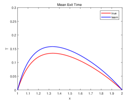
(a) Mean exit time

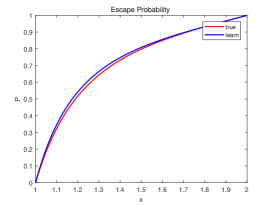
(b) Escape probability

Figure 1: 1-D double-well system driven by Brownian motion. (a) Mean exit time for the true system and the learned system. (b) Escape probability for the true system and the learned system.

Example 4.2

Consider a two-dimensional system with two-dimensional Brownian motion

$$dX_{t}=(3X_{t}-Y_{t}^{2})dt+X_{t}dW_{t},$$

$$dY_{t}=(2X_{t}+Y_{t})dt+Y_{t}d\tilde{W}_{t},$$ (4.3)

where $W_{t}$ and $\tilde{W}_{t}$ are two disjoint independent scalar real-value Brownian motion. The generator of this system is easy to know from (2.5) by taking $b_{1}(x,y)=3x-y^{2}$, $b_{2}(x,y)=2x+y$ and

$\sigma_{1}=\left[{\begin{array}[]{*{20}{c}}x&0\\ 0&y\end{array}}\right].$

Similar to Example 4.1, We use the EDMD algorithm to data, from (4.2), to learn their governing law. The data set has $10^{6}$ initial points on $x\in(-1,1)\times(-1,1)$ drawn from a uniform grid, which constitute $X$, and their positions after $\Delta t=0.01$, which constitute $Y.$ The sample paths were obtained by Euler-Maruyama method. The dictionary chosen is a polynomial with order up to 3.
As can be seen from Table 2 and Table 3, it is very close to the true parameters. Using the stochastic differential equation coefficients learned from the data, we obtained mean exit time and escape probability by solving the partial differential equations (2.13) and (2.2). We can see from Fig.2(a), Fig.2(b), Fig.3(a) and Fig.3(b) that they are almost identical. The mean error of mean exit time and escape time are $0.0041$ and $0.0575$. These results show that we still can obtain the accurate mean exit time and escape probability in high dimension from data.

Table 2: Identified drift terms for 2-D system driven by Brownian motion.

basis	true	learning
$1$	0	0
$x$	3	2.9837
$y$	0	0
$x^{2}$	0	0
$xy$	0	0
$y^{2}$	-1	-1.0026
$x^{3}$	0	0
$x^{2}y$	0	0
$xy^{2}$	0	0
$y^{3}$	0	0

(a) Drift term $b_{1}$

basis	true	learning
$1$	0	0
$x$	2	2.0391
$y$	1	1.0056
$x^{2}$	0	0
$xy$	0	0
$y^{2}$	0	0
$x^{3}$	0	0
$x^{2}y$	0	0
$xy^{2}$	0	0
$y^{3}$	0	0

(b) Drift term $b_{2}$

Table 3: Identified diffusion terms for 2-D system driven by Brownian motion.

basis	true	learning
$1$	0	0
$x$	0	0
$y$	0	0
$x^{2}$	1	1.2835
$xy$	0	0
$y^{2}$	0	0
$x^{3}$	0	0
$x^{2}y$	0	0
$xy^{2}$	0	0
$y^{3}$	0	0

(a) Diffusion term $\sigma_{11}^{2}$

basis	true	learning
$1$	0	0
$x$	0	0
$y$	0	0
$x^{2}$	0	0
$xy$	0	0
$y^{2}$	1	0.9750
$x^{3}$	0	0
$x^{2}y$	0	0
$xy^{2}$	0	0
$y^{3}$	0	0

(b) Diffusion term $\sigma_{22}^{2}$

(a) Mean exit time for the true system

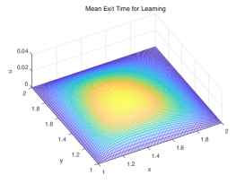
(b) Mean exit time for the learning system

Figure 2: 2-D system driven by Brownian motion. (a) Mean exit time for the true system. (b) Mean exit time for the learned system.

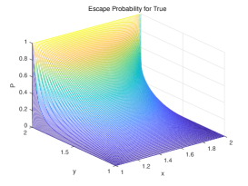
(a) Escape probability for the true system

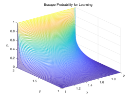
(b) Escape probability for the learning system

Figure 3: 2-D system driven by Brownian motion. (a) Escape probability for the true system. (b) Escape probability for the learned system.

4.2 Dynamical systems with Lévy motion

We will demonstrate that we can obtain mean exit time and escape probability from data, simulated for systems with rotationally invariant $\alpha$-stable Lévy motion. In what follows computations, we take that the stable index $\alpha=1$ and the jump measure $\tilde{\nu}(dx)=I_{\{\|x\|<c\}}\frac{dx}{|x|^{d+\alpha}}$ with $c=1$.

Example 4.3

Consider a scalar double-well system with scalar Lévy motion as follows

$$dX_{t}=(4X_{t}-X_{t}^{3})dt+X_{t}dW_{t}+d\tilde{L}_{t}^{\alpha},$$ (4.4)

where $W_{t}$ is a scalar real-value Brownian motion and $L_{t}^{\alpha}$ is a Lévy motion with triple $(0,0,\tilde{\nu})$ as we said in Section 2.1. The generator of this system is easy to know from (2.1) by taking $b(x)=4x-x^{3}$,$\sigma_{1}=x$ and $\sigma_{2}=1$.
Thus we have

$$(\mathcal{L}f)(x) =(4x-x^{3})f^{{}^{\prime}}(x)+\frac{1}{2}x^{2}f^{{}^{\prime\prime}}(x)$$

$$+C_{\alpha}\int_{\mathbb{R}\backslash\{0\}}[f(x+y)-f(x)]I_{\{\|y\|<c\}}(y)\,\frac{dy}{|y|^{1+\alpha}}.$$ (4.5)

The data set has $10^{6}$ initial points on $x\in(-2,2)$ drawn from a uniform grid, which constitute $X$, and their positions after $\Delta t=0.01$, which constitute $Y.$ The sample paths were obtained by Euler-Maruyama method. The dictionary chosen is a polynomial with order up to 5.
Notice that we have non-Gaussian noise here. As can be seen from Table 4, it is very close to the true parameters. In addition, the diffusion term squared of Lévy motion, learning from data, is equal to 1.0955. It’s close to the true coefficient 1. Using the stochastic differential equation coefficients learned from the data, we obtained mean exit time and escape probability by solving the partial differential equations (2.8), (2.9) and (2.2). We can see from Fig.4(a) and Fig.4(b) that they are almost identical.

Table 4: Identified coefficients for 1-D double-well system driven by Lévy motion.

basis	true	learning
$1$	0	0
$x$	4	4.0716
$x^{2}$	0	0
$x^{3}$	-1	-1.0966
$x^{4}$	0	0
$x^{5}$	0	0

(a) Drift term

basis	true	learning
$1$	0	0
$x$	0	0
$x^{2}$	1	0.9862
$x^{3}$	0	0
$x^{4}$	0	0
$x^{5}$	0	0

(b) Diffusion term $\sigma_{1}^{2}$

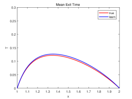
(a) Mean exit time

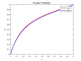
(b) Escape probability

Figure 4: 1-D double-well system driven by Lévy motion. (a) Mean exit time for the true system and the learned system. (b) Escape probability for the true system and the learned system.

Example 4.4

Consider a two-dimensional system

$$dX_{t}=(3X_{t}-Y_{t}^{2})dt+X_{t}dW_{t}+d\tilde{L}_{1,t}^{\alpha},$$

$$dY_{t}=(2X_{t}+Y_{t})dt+Y_{t}d\tilde{W}_{t}+d\tilde{L}_{2,t}^{\alpha},$$ (4.6)

where $W_{t}$, $\tilde{W}_{t}$, $\tilde{L}_{1,t}$ and $\tilde{L}_{2,t}$ are four disjoint independent scalar real-value Brownian motions and Lévy motions as we said in Section 2.1. Note that we still assume that the jump size of Lévy motions are bounded. The generator of this system is easy to know from (2.1) by taking $b_{1}(x,y)=3x-y^{2}$, $b_{2}(x,y)=2x+y$ and

$\sigma_{1}=\left[{\begin{array}[]{*{20}{c}}x&0\\ 0&y\end{array}}\right],$ $\sigma_{2}=\left[{\begin{array}[]{*{20}{c}}1&0\\ 0&1\end{array}}\right].$

For this 2-D system, the data set has $10^{6}$ initial points on $x\in(-1,1)\times(-1,1)$ drawn from a uniform grid, which constitute $X$, and their positions after $\Delta t=0.01$, which constitute $Y.$ The sample paths were obtained by Euler-Maruyama method. The dictionary chosen is a polynomial with order up to 3.
As can be seen from Table 5 and Table 6, it is very close to the true parameters. In addition, the diffusion term squared of Lévy motion, learning from data, is equal to $[1.0710,0;0,1.0370]$. It’s close to the true coefficient $[1,0;0,1]$. Using the stochastic differential equation coefficients learned from the data, we obtained mean exit time and escape probability by solving the partial differential equations (2.8), (2.9) and (2.2). We can see from Fig.5(a), Fig.5(b), Fig.6(a) and Fig.6(b) that they are almost identical. The mean error of mean exit time and escape time are $6.2429e-04$ and $0.0128$.

Remark 4.5

These examples show that although we use finite dimensional matrices to approximate infinite dimensional linear operators, we can still accurately capture the mean exit time and escape probability of the corresponding stochastic dynamical system. i.e., we can discover deterministic indexes (e.g., mean exit time, escape probability) to gain insights about transition phenomena from data for stochastic dynamical systems under Gaussian noise or non-Gaussian noise.

Table 5: Identified drift terms for 2-D system driven by Lévy motion.

basis	true	learning
$1$	0	0
$x$	3	3.1096
$y$	0	0
$x^{2}$	0	0
$xy$	0	0
$y^{2}$	-1	-0.9587
$x^{3}$	0	0
$x^{2}y$	0	0
$xy^{2}$	0	0
$y^{3}$	0	0

(a) Drift term $b_{1}$

basis	true	learning
$1$	0	0
$x$	2	2.0882
$y$	1	1.0324
$x^{2}$	0	0
$xy$	0	0
$y^{2}$	0	0
$x^{3}$	0	0
$x^{2}y$	0	0
$xy^{2}$	0	0
$y^{3}$	0	0

(b) Drift term $b_{2}$

Table 6: Identified drift terms for 2-D system driven by Lévy motion.

basis	true	learning
$1$	0	0
$x$	0	0
$y$	0	0
$x^{2}$	1	0.9668
$xy$	0	0
$y^{2}$	0	0
$x^{3}$	0	0
$x^{2}y$	0	0
$xy^{2}$	0	0
$y^{3}$	0	0

(a) Diffusion term $\sigma_{11}^{2}$

basis	true	learning
$1$	0	0
$x$	0	0
$y$	0	0
$x^{2}$	0	0
$xy$	0	0
$y^{2}$	1	1.0213
$x^{3}$	0	0
$x^{2}y$	0	0
$xy^{2}$	0	0
$y^{3}$	0	0

(b) Diffusion term $\sigma_{22}^{2}$

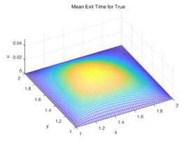
(a) Mean exit time for the true system

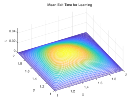
(b) Mean exit time for the learning system

Figure 5: 2-D system driven by Lévy motion. (a) Mean exit time for the true system. (b) Escape probability for the learned system.

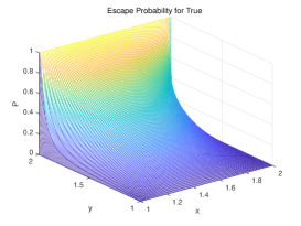
(a) Escape probability for the true system

(b) Escape probability for the learning system

Figure 6: 2-D system driven by Lévy motion. (a) Escape probability for the true system. (b) Escape probability for the learned system.

5 Discussion

We have presented an approach for obtaining deterministic indexes about transition phenomena of non-Gaussian stochastic dynamical systems from data. In particular, we have identified the coefficients from the stochastic differential equations with non-Gaussian Lévy motion and extracted information about transition phenomena (e.g. mean exit time and escape probability) from the data of the stochastic system . Here we have applied the Koopman analysis framework to deal with stochastic systems with Lévy motion.

Existing relevant works focused on either deterministic systems, or stochastic systems with Gaussian Brownian motion, including our earlier work [22], where the stochastic governing law is directly learned from data.

In fact, we can further obtain transition probability density functions of the stochastic dynamical systems, because we can additionally solve the associated Fokker-Planck equations.

However, there are several challenges for further investigation. First, so far there is no rigorous error analysis for the finite-dimensional approximation of infinite dimensional linear operators. Generally speaking, finite-dimensional approximation is more effective when operators have pure point spectra. However, when the linear operator has a continuous spectrum, there is still no good way to deal with it. Second, how to choose an appropriate basis of functions is a challenge. Third, we have noticed that stochastic dynamical systems need more simulated data than deterministic dynamical systems, in order to extract transition dynamics. Hence, reducing the demand for data is worth of further investigation. Fourth, our method requires data on system states. If we only have observation and this observation function can be expanded using basis, our method still can work. Otherwise, we have to use other suitable methods based on observations. For example, our earlier work [26] demonstrated a method to learn stochastic governing laws with observations not on system states. Finally, our method is not valid when the Lévy noise is non-diagonal matrix or multiplicative, because we can not separate non-Gaussian noise from Gaussian noise.

Data Availability Statements

The data that support the findings of this study are openly available in GitHub, reference number [27].

Appendix

Lévy motions
Let $L=(L_{t},t\geq 0)$ be a stochastic process defined on a probability space $(\Omega,\mathcal{F},P)$. We say that L is a Lévy motion if:

• $L_{0}=0(a.s.)$;

• $L$ has independent and stationary increments;

• $L$ is stochastically continuous, i.e., for all $a>0$ and for all $s\geq 0$

  $$\lim\limits_{t\to s}P(|L_{t}-L_{s}|>a)=0.$$

Characteristic functions
For a Lévy motion $(L_{t},t\geq 0)$, we have the Lévy-Khinchine formula,

$$\mathbb{E}[e^{i(u,L_{t})}]=exp\{t[i(b,u)-\frac{1}{2}(u,Au)+\int_{\mathbb{R}^{d}\backslash\{0\}}[e^{i(u,y)}-1-i(u,y)I_{\{\|y\|<1\}}(y)]\,\nu(dy)]\},$$

for each $t\geq 0$, $u\in\mathbb{R}^{d}$, where $(b,A,\nu)$ is the triple of Lévy motion $(L_{t},t\geq 0)$.

Theorem (The Lévy-Itô decomposition) If $(L_{t},t\geq 0)$ is a Lévy motion with $(b,A,\nu)$, then there exists $b\in\mathbb{R}^{d}$, a Brownian motion $B_{A}$ with covariance matrix $A$ and an independent Poisson random measure $N$ on $\mathbb{R}^{+}\times(\mathbb{R}^{d}-\{0\})$ such that, for each $t\geq 0$,

$$L_{t}=bt+B_{A}(t)+\int_{0<|x|<c}x\,\tilde{N}(t,dx)+\int_{|x|\geq c}x\,N(t,dx),$$

where $\int_{|x|\geq c}x\,N(t,dx)$ is a Poisson integral and $\int_{0<|x|<c}x\,\tilde{N}(t,dx)$ is a compensated Poisson integral defined by

$$\int_{0<|x|<c}x\,\tilde{N}(t,dx)=\int_{0<|x|<c}x\,N(t,dx)-t\int_{0<|x|<c}x\,\nu(dx).$$

Specially, in our work, we assume that the components of a $d-$dimensional Lévy motion have triple $(0,0,\tilde{\nu})$. i.e.,

$$(\tilde{L}_{t}^{\alpha})_{i}=\int_{0<|x|<c}x\,\tilde{N}(t,dx),$$

where $i=1,2,\ldots,d$, $x\in\mathbb{R}$ and $\tilde{\nu}(dx)=C_{\alpha}I_{\{\|x\|<c\}}(x)\frac{dx}{|x|^{1+\alpha}}$. See [21, 20].

References

- [1] A. J. Chorin and F. Lu. Discrete approach to stochastic parametrization and dimension reduction in nonlinear dynamics. Proceedings of the National Academy of Sciences 112.32(2015):9804-9809.
- [2] A. Ruttor, P. Batz, and M. Opper. Approximate Gaussian process inference for the drift of stochastic differential equations. International Conference on Neural Information Processing Systems Curran Associates Inc. 2013.
- [3] C. A. Garc a, P. Félix, J. Presedo, D. g. Márquez. Nonparametric estimation of stochastic differential equations with sparse Gaussian processes. Physical Review E 96.2(2017):022104.
- [4] S. L. Brunton, J.L. Proctor , and J.N. Kutz. Discovering governing equations from data by sparse identification of nonlinear dynamical systems. Proceedings of the National Academy of Sciences (2016):201517384.
- [5] K. Champion, B. Lusch, J. N. Kutz, S. L. Brunton. Data-driven discovery of coordinates and governing equations. Proceedings of the National Academy of Sciences (2019):1906995116.
- [6] M. Reza Rahimi Tabar. Analysis and Data-Based Reconstruction of Complex Nonlinear Dynamical Systems, Springer, 2019.
- [7] P. J. Schmid. Dynamic Mode Decomposition of numerical and experimental data. Journal of Fluid Mechanics 656.10(2008):5-28.
- [8] M. O. Williams, I. G. Kevrekidis, and C.W. Rowley. A Data-Driven Approximation of the Koopman Operator: Extending Dynamic Mode Decomposition. Journal of Nonlinear Science 25.6(2015):1307-1346.
- [9] N. Takeishi, Y. Kawahara , and T. Yairi. Subspace dynamic mode decomposition for stochastic Koopman analysis. Physical Review E 96.3(2017):033310.
- [10] A. N. Riseth, J.P. Taylor-King. Operator Fitting for Parameter Estimation of Stochastic Differential Equations arXiv preprint arXiv:1709.05153v2, (2018).
- [11] I. Mezić. Spectrum of the Koopman Operator, Spectral Expansions in Functional Spaces, and State Space Geometry. arXiv preprint arXiv:1702.07597v2, (2019).
- [12] S. Klus, F. Nüske, S. Peitz, J H. Niemann, C. Clementi, C. Schütte. Data-driven approximation of the Koopman generator: Model reduction, system identification, and control. Physica D: Nonlinear Phenomena, Vol 406, 132416 (2020).
- [13] M. Dellnitz, G. Froyland, C. Horenkamp, K. Padberg-Gehle, A. Sen Gupta. Seasonal variability of the subpolar gyres in the Southern Ocean: a numerical investigation based on transfer operators. Nonlinear Processes in Geophysics, 16, 655-664, 2009.
- [14] G. Froyland, O. Junge, P. Koltai. Estimating long-term behavior of flows without trajectory integration: the infinitesimal generator approach. SIAM J. NUMER. ANAL, Vol. 51, No. 1, pp. 223-247 (2013).
- [15] S. Klus, P. Koltai, C. Schütte. On the numerical approximation of the Perron- Frobenius and Koopman operator. Journal of Computational Dynamics, Vol. 3, No. 1, pp. 51-79 (2016).
- [16] S. Klus, F. Nüske, P. Koltai, H. Wu, I, Kevrekidis, C. Schütte, F. Noé. Data-Driven Model Reduction and Transfer Operator Approximation. J Nonlinear Sci (2018) 28:985 C1010.
- [17] P. Metzner, E. Dittmer, T. Jahnke, C. Schütte. Generator estimation of Markov jump processes. Journal of Computational Physics, 227(2007) 353-37.
- [18] A. Tantet, F R. van der Burgt, H A. Dijkstra. An early warning indicator for atmospheric blocking events using transfer operators. Chaos 25 036406 (2015).
- [19] E H. Thiede, D. Giannakis , A R. Dinner, J. Weare. Galerkin approximation of dynamical quantities using trajectory data. J Chem. Phys. 150, 244111(2019).
- [20] J. Duan. An Introduction to Stochastic Dynamics, Cambridge University Press, New York, 2015.
- [21] D. Applebaum. Lévy Processes and Stochastic Calculus, second ed., Cambridge University Press, 2009.
- [22] D. Wu, M. Fu and J. Duan. Discovering mean residence time and escape probability from data of stochastic dynamical systems. Chaos 29 093122 (2019).
- [23] T. Gao, J. Duan, X. Li, R. Song. Mean Exit Time and Escape Probability for Dynamical Systems Driven by Lévy Noises. SIAM Journal on Scientific Computing 36.3(2012).
- [24] X. Chen, F. Wu, J. Duan, J. Kurths, X. Li. Most probable dynamics of a genetic regulatory network under stable Lévy noise. Applied Mathematics and Computation, 348:425-436, 2018.
- [25] X. Sun, X. Li, Y. Zheng. Governing equations for probability densities of Marcus stochastic differential equations with Lévy noise. Stochastics and Dynamics, Vol. 17, No. 5(2017).
- [26] J. Duan, T. Gao, G. He. Quantifying Model Uncertainties in the Space of Probability Measures. arXiv preprint arXiv:1204.0855v1, (2012).
- [27] Y. Lu. Code. GitHub, https://github.com/Yubin-Lu/Discovering-transition-phenomena-from-data-of-stochastic-dynamical-systems, 2020.