Linearly Convergent Algorithm with Variance Reduction for Distributed Stochastic Optimization

Abstract

This paper considers a distributed stochastic strongly convex optimization, where agents over a network aim to cooperatively minimize the average of all agents’ local cost functions. Due to the stochasticity of gradient estimation and distributedness of local objective, fast linearly convergent distributed algorithms have not been achieved yet. This work proposes a novel distributed stochastic gradient tracking algorithm with variance reduction, where the local gradients are estimated by an increasing batch-size of sampled gradients. With an undirected connected communication graph and a geometrically increasing batch-size, the iterates are shown to converge in mean to the optimal solution at a geometric rate (achieving linear convergence). The iteration, communication, and oracle complexity for obtaining an $\epsilon$-optimal solution are established as well. Particulary, the communication complexity is $\mathcal{O}(\ln(1/\epsilon))$ while the oracle complexity (number of sampled gradients) is $\mathcal{O}(1/\epsilon^{2})$, which is of the same order as that of centralized approaches. Hence, the proposed scheme is communication-efficient without requiring extra sampled gradients. Numerical simulations are given to demonstrate the theoretic results.

I Introduction

Distributed optimization has been extensively studied in recent years due to its wide applications in sensor networks [1, 2], power systems [3, 4], distributed estimation and control [5, 6, 7]. Various distributed optimization methods have been developed, including primal domain methods [8, 9], dual domain methods [10, 11], and primal-dual domain methods [12, 13, 14]. Please refer to the survey [15] for more references.

This paper aims to provide a fast and communication-efficient algorithm for distributed stochastic optimization. We propose a stochastic variant of the distributed gradient tracking scheme [9], where each agent is equipped with an auxiliary variable to track the dynamical average gradient in addition to the solution estimate. To achieve fast convergence and save communication cost (which is usually hundreds times of local computation cost), an adaptive sampling method is incorporated into the scheme. The main contributions of the paper are given as follows.

• We first combine the distributed stochastic gradient tracking algorithm with adaptive variance reduction, where each agent estimates its local gradients with an increasing batchsize of sampled gradients. Then each agent takes a weighted average of its neighbors’ estimates and moves towards the negative direction of its local noisy gradient estimation.

• When each agent’s local objective function is strongly convex with Lipschitz-continuous gradient and the sample size for gradient estimation adaptively increases at a geometric rate, the proposed scheme with a constant stepsize can generate geometrically/linearly convergent iterates.

• Furthermore, it is shown that the iteration, communication, and oracle complexity for each agent $i$ to obtain an $\epsilon$-optimal solution are $\mathcal{O}(\ln(1/\epsilon))$, $\mathcal{O}(|\mathcal{N}_{i}|\ln(1/\epsilon))$, $\mathcal{O}(1/\epsilon^{2})$, respectively, where $|\mathcal{N}_{i}|$ denotes the number of agent $i$’s neighbors. Compared with existing distributed methods, the scheme saves the communication cost without increasing the overall sampling burden.

Literature review on distributed stochastic optimization. Considerable works have been done in distributed stochastic optimization, e.g., distributed stochastic subgradient projection algorithm [16], distributed asynchronous algorithm [17], and distributed primal-dual method [18]. In the following, we review some literature on the convergence rate and complexity analysis of distributed stochastic strongly convex optimization. The work [19] proposed a distributed stochastic gradient method over a random network and established the convergence rate of $\mathcal{O}(1/k)$ in a mean-squared sense. A distributed stochastic mirror descent method with rate $\mathcal{O}(\ln(k)/k)$ was given in [20] for non-smooth functions, while a stochastic subgradient descent with rate $\mathcal{O}(n\sqrt{n}/k)$ was proved in [21]. The work [22] proposed a subgradient-push method over time-varying directed graphs and obtained a rate $\mathcal{O}(\ln(k)/k)$. A distributed stochastic gradient tracking method with a constant stepsize was designed in [23], which only showed that the iterates are attracted to a neighborhood of the optimal solution in expectation with an exponential rate, however, the exact convergence can not be achieved yet.

This work considers minimizing smooth objectives over an undirected connected network. Instead of decaying stepsizes in [19, 20, 21, 22], we adopt a constant stepsize and achieve exact and fast convergence. By progressively reducing the variance of gradient noises through increasing sample size, the derived iteration complexity matches that of centralized approaches for deterministic optimization, achieving superior complexity bounds than the prior works [19, 20, 21, 22, 23]. Moreover, the approach can significantly reduce the communication rounds, meanwhile the oracle complexity can be comparable with existing distributed stochastic gradient algorithms. To the best of our knowledge, this is the first work that achieves a linear convergence rate for distributed strongly convex stochastic optimization.

The paper is organized as follows. A distributed stochastic gradient tracking algorithm with variance reduction is proposed in Section II. The geometric convergence rate along with the complexity bounds are established in Section III. The numerical studies are presented in Section IV, while concluding remarks are given in Section V.

Notations. Depending on the argument, $|\cdot|$ stands for the absolute value of a real number or the cardinality of a set. The Euclidean norm of a vector or a matrix is denoted as $\|\cdot\|_{2}$ or $\|\cdot\|$. Let $\otimes$ denote the Kronecker product. Let $\mathbf{1}$ denote the column vectors with all entries equal to 1 and $I_{d}$ denote the $d\times d$ identity matrix. An undirected graph is denoted by $\mathcal{G}=\{\mathcal{V},\mathcal{E}\},$ where $\mathcal{V}=\{1,\dots,n\}$ is a finite set of nodes and each edge $(i,j)\in\mathcal{E}$ is an unordered pair of two distinct nodes $i,j$. A path in $\mathcal{G}$ from $v_{1}$ to $v_{p}$ is a sequence of distinct nodes, $v_{1}\dots v_{p}$, such that $(v_{m},v_{m+1})\in\mathcal{E}$ for all $m=1,\dots,p-1$. The graph $\mathcal{G}$ is termed connected if for any two distinct nodes $i,j\in\mathcal{V}$, there is a path between them. The set of node $i$’s neighboring nodes, denoted by $\mathcal{N}_{i}$, is defined as $\mathcal{N}_{i}\triangleq\{j\in\mathcal{V}:(i,j)\in\mathcal{E}\}$. Define the adjacency matrix of graph $\mathcal{G}$ as $A=[a_{ij}]_{i,j=1}^{n}$, where $a_{ij}>0$ if $j\in\mathcal{N}_{i}$ and $a_{ij}=0$ otherwise.

II Problem Statement and Algorithm Design

In this section, we first formulate a distributed stochastic optimization problem with some assumptions. Then we propose a fully distributed variable sample-size stochastic gradient tracking algorithm.

II-A Problem Formulation

We consider a network of $n$ agents indexed as $\mathcal{V}=\big{\{}1,\dots,n\big{\}}$, where the agents interaction is described by an undirected graph $\mathcal{G}=\{\mathcal{V},\mathcal{E}\}$. Agent $i\in\mathcal{V}$ has an expectation-valued cost function $f_{i}(x)\triangleq\mathbb{E}_{\xi_{i}}[h_{i}(x,\xi_{i})]$, where $x\in\mathbb{R}^{d}$, the random vector $\xi_{i}:{\Omega_{i}}\to\mathbb{R}^{m_{i}}$ is defined on the probability space $({\Omega_{i}},{\cal F}_{i},\mathbb{P})$, and $h:\mathbb{R}^{d}\times\mathbb{R}^{m_{i}}\to\mathbb{R}$ is a scalar-valued function. The agents in the network need to cooperatively find an optimal solution that minimizes the average of all agents’ local cost functions, i.e.,

$$\begin{split}\min_{x\in\mathbb{R}^{d}}F(x)\triangleq{1\over n}\sum_{i=1}^{n}f_{i}(x).\end{split}$$ (1)

We aim to design a distributed algorithm to drive all agents’ iterates to the optimal solution, explore its convergence rate, and establish the complexity bounds for obtaining an optimal solution with a prescribed accuracy. Below are the assumptions on the communication graph and cost functions.

Assumption 1

The undirected graph $\mathcal{G}$ is connected, and its adjacency matrix $A=[a_{ij}]_{i,j=1}^{n}$ is symmetric with the weights $a_{ij}$ satisfying the following condition:

$$\sum_{i=1}^{n}a_{ij}=1,\quad\forall j\in\mathcal{V}.$$ (2)

With Assumption 1, the adjacency matrix $A$ of the connected communication graph is doubly stochastic. It has been shown in [24] that the spectral radius $\sigma_{A}$ of $A-\mathbf{1}\mathbf{1}^{T}/n$ satisfies $\sigma_{A}\in(0,1)$.

Assumption 2

For each agent $i\in\mathcal{V},$ its cost function $f_{i}(x)$ is $\eta$-strongly convex and its gradient function is $L$-Lipschitz continuous, i.e., for any $x_{1},x_{2}\in\mathbb{R}^{d}$:
(i) $(\nabla f_{i}(x_{1})-\nabla f_{i}(x_{2}))^{T}(x_{1}-x_{2})\geq\eta\|x_{1}-x_{2}\|^{2},$
(ii) $\|\nabla f_{i}(x_{1})-\nabla f_{i}(x_{2})\|\leq L\|x_{1}-x_{2}\|.$

By Assumption 2 and definition $F(x)={1\over n}\sum_{i=1}^{n}f_{i}(x)$, $F(x)$ is $\eta$-strongly convex and its gradient function is $L$-Lipschitz continuous. Then problem (1) has a unique optimal solution, denoted by $x^{*}$. Hence, $\nabla F(x^{*})=0$ by the first-order optimality condition.

Suppose there exists a stochastic first-order oracle for each agent $i\in\mathcal{V}$ such that for any given $x,\xi$, a sampled gradient $\nabla h_{i}(x,\xi)$ is returned, which is an unbiased estimator of $\nabla f_{i}(x)$ with bounded second-order moment. Here is the assumption on the stochastic first-order oracle.

Assumption 3

There exists a constant $\nu>0$ such that the following holds for each $i\in\mathcal{V}$ and any given $x\in\mathbb{R}^{d}$,

$$\mathbb{E}_{\xi_{i}}[\nabla h_{i}(x,\xi_{i})]=\nabla f_{i}(x),{~{}\rm and~{}}$$

$$\mathbb{E}_{\xi_{i}}[\|\nabla h_{i}(x,\xi_{i})-\nabla f_{i}(x)\|^{2}]\leq\nu^{2}.$$

II-B A Distributed Stochastic Gradient Tracking Algorithm with Variance Reduction

The discrete time is slotted at $k=0,1,2,\dots$. Each agent $i$ at time $k$ maintains two estimates $x_{i}(k)$ and $y_{i}(k)$, where $x_{i}(k)$ and $y_{i}(k)$ are used to estimate the optimal solution and to track the average gradient, respectively. Since the exact gradient of each expectation-valued cost function $f_{i}(x)$ is unavailable, we approximate it by averaging through a variable batch-size of sampled gradients:

$$\tilde{g}_{i}(x_{i}(k))={1\over N(k)}\sum_{p=1}^{N(k)}\nabla h_{i}(x_{i}(k),\xi^{p}_{i}(k)),\quad\forall k\geq 0,$$ (3)

where $N(k)$ is the number of sampled gradients utilized at time $k$ and the samples $\{\xi^{p}_{i}(k)\}_{p=1}^{N(k)}$ are randomly and independently generated from the probability space $({\Omega_{i}},{\cal F}_{i},\mathbb{P})$. The gradient estimate given by (3) is an unbiased estimate of the exact gradient, and the variance of the gradient noise will be progressively reduced by increasing the batch-size. By combining the distributed gradient tracking scheme [9] with a variance reduction scheme, we obtain Algorithm 1. We will specify the selection of the constant steplength $\alpha$ and the batch-size $N(k)$ upon convergence analysis.

Algorithm 1 A distributed variable sample-size stochastic gradient tracking algorithm

Initialization: Set $k:=0$. For any $i=1,\ldots,n$, let $y_{i}(0)=\tilde{g}_{i}(x_{i}(0))$ with arbitrary initial $x_{i}(0)\in\mathbb{R}^{d}$.

Iterate until convergence.

Each agent $i=1,\cdots,n$ updates its estimates as follows:

$$x_{i}(k+1) =\sum_{j\in\mathcal{N}_{i}}a_{ij}x_{j}(k)-\alpha y_{i}(k),$$ (4a)

$$y_{i}(k+1) =\sum_{j\in\mathcal{N}_{i}}a_{ij}y_{j}(k)+\tilde{g}_{i}(x_{i}(k+1))-\tilde{g}_{i}(x_{i}(k)),$$ (4b)

where $\alpha>0$ is the steplength and $\tilde{g}_{i}(x_{i}(k))$ is given in (3).

Note that for each agent $i\in\mathcal{V},$ the implementation of Eqn. (4a) requires its neighbors’ estimates of the optimal solution $\{x_{j}(k)\}_{j\in\mathcal{N}_{i}}$, while the update of $y_{i}(k+1)$ characterized by Eqn. (4b) uses its local gradient estimate as well as its neighbors’ information $\{y_{j}(k)\}_{j\in\mathcal{N}_{i}}$ to asymptotically track the dynamical average gradient across the network. Therefore, Algorithm 1 is a fully distributed algorithm since the update of each agent merely uses its local data and its neighboring information.

III Convergence Analysis

In this section, we show the geometric convergence rate for Algorithm 1 when the batchsize is increased at a geometric rate, and establish the complexity bounds for obtaining an $\epsilon$-optimal solution.

III-A Preliminary Lemma

Define the gradient observation noise as follows:

$$w_{i}(k)\triangleq\tilde{g}_{i}(x_{i}(k))-\nabla f_{i}(x_{i}(k)).$$ (5)

We further define

$$\begin{array}[]{ll}&x(k)\triangleq\big{(}x_{1}(k)^{T},\cdots,x_{n}(k)^{T}\big{)}^{T},\\ &y(k)\triangleq\big{(}y_{1}(k)^{T},\cdots,y_{n}(k)^{T}\big{)}^{T},\\ &\nabla(k)\triangleq\big{(}\nabla f_{1}(x_{1}(k))^{T},\cdots,\nabla f_{n}(x_{n}(k))^{T}\big{)}^{T},\\ &w(k)\triangleq\big{(}w_{1}(k)^{T},\cdots,w_{n}(k)^{T}\big{)}^{T}.\end{array}$$ (6)

Then Algorithm 1 is written in a compact form:

$$x(k+1) =(A\otimes I_{d})x(k)-\alpha y(k)$$ (7a)

$$y(k+1) =(A\otimes I_{d})y(k)+\nabla(k+1)$$

$$\quad+w(k+1)-\nabla(k)-w(k).$$ (7b)

Define the average of agents’ estimates of the optimal solution and the averaged gradient across the network as follows for any $k\geq 0$:

$$\bar{x}(k)={1\over n}\sum_{i=1}^{n}x_{i}(k){\rm~{}and}~{}\bar{y}(k)={1\over n}\sum_{i=1}^{n}y_{i}(k).$$ (8)

We start to analyze the algorithm performance by characterizing the interactions among the three error sequences: (i) distance from the average estimate to the optimal solution $\|\bar{x}(k)-x^{*}\|;$ (ii) consensus error $\|x(k)-(\mathbf{1}\otimes I_{d})\bar{x}(k)\|$; and (iii) consensus error of the gradient trackers $\|y(k)-(\mathbf{1}\otimes I_{d})\bar{y}(k)\|$. We bound the three error sequences in terms of the linear combinations of their past values in the following lemma, of which the proofs can be found in Appendix.

Lemma 1

Suppose Assumptions 1 and 2 hold. Let the sequences $\{x(k)\}$ and $\{y(k)\}$ be generated by Algorithm 1 with $0<\alpha\leq{2\over\eta+L}.$ Define the following vector and matrix:

$$\begin{split}z(k)&\triangleq\begin{pmatrix}\|\bar{x}(k)-x^{*}\|\\ \|x(k)-(\mathbf{1}\otimes I_{d})\bar{x}(k)\|\\ \|y(k)-(\mathbf{1}\otimes I_{d})\bar{y}(k)\|\end{pmatrix},\\ J(\alpha)&\triangleq\begin{pmatrix}1-\alpha L&\alpha{L\over\sqrt{n}}&{0}\\ {0}&\sigma_{A}&\alpha\\ \alpha\sqrt{n}L^{2}&L\|A-I_{n}\|+\alpha L^{2}&\sigma_{A}+\alpha L\end{pmatrix}.\end{split}$$ (9)

Then the following inequalities hold for any $k\geq 0$:

$$\begin{split}&z(k+1)\leq J(\alpha)z(k)\\ &+\begin{pmatrix}{\alpha\over n}\sum_{i=1}^{n}\left\|w_{i}(k)\right\|\\ {0}\\ \|w(k+1)-w(k)\|+{\alpha L\over\sqrt{n}}\sum_{i=1}^{n}\left\|w_{i}(k)\right\|\end{pmatrix}.\end{split}$$ (10)

III-B Linear convergence rate analysis

We now give the linear convergence rate result.

Theorem 1

Suppose Assumptions 1, 2, and 3 hold. Let $\{x(k)\}$ and $\{y(k)\}$ be generated by Algorithm 1 with $0<\alpha\leq{2\over\eta+L}.$ Set $N(k)=\lceil q^{-2k}\rceil$ for some $q\in(0,1).$ Take $\alpha$ such that the spectral radius of the matrix $J(\alpha)$, denoted by $\rho(J(\alpha))$, is strictly smaller than 1. Then $z(k)$ converges to zero in mean at a geometric rate, that is,

$$\mathbb{E}[\|z(k)\|] \leq\rho(J(\alpha))^{k}\|\mathbb{E}[z(0)]\|+{C\over q-\rho(J(\alpha))}q^{k},$$

$$\qquad\qquad{\rm when~{}}q>\rho(J(\alpha)),$$ (11a)

$$\mathbb{E}[\|z(k)\|] \leq\rho(J(\alpha))^{k}\|\mathbb{E}[z(0)]\|+{C\over\rho(J(\alpha))-q}\rho(J(\alpha))^{k},$$

$$\qquad\qquad{~{}\rm when~{}}q<\rho(J(\alpha)),$$ (11b)

where $C\triangleq\nu\sqrt{\alpha^{2}+n(1+q+\alpha L)^{2}}.$

Proof. We first split the matrix $J(\alpha)$ into the sum of a fixed matrix and another perturbation matrix as a function $\alpha$:

$$\begin{array}[]{ll}J(\alpha)&\triangleq\begin{pmatrix}1&0&0\\ 0&\sigma_{A}&0\\ 0&L\|A-I_{n}\|&\sigma_{A}\end{pmatrix}+\alpha\begin{pmatrix}-L&{L\over\sqrt{n}}&0\\ 0&0&1\\ \sqrt{n}L^{2}&L^{2}&L\end{pmatrix}\\ &:=J(0)+\alpha E.\end{array}$$

Because $\sigma_{A}\in(0,1),$ the spectral radius of $J(0)$ is 1 and the corresponding right and left eigenvector to the eigenvalue of 1 of $J(0)$ is $(1,0,0)^{T}$. Because the eigenvalues of a matrix are a continuous function of its entries, we are able to choose some sufficiently small $\alpha$ such that the spectral radius of $J(\alpha)$ is strictly smaller than 1 (see [25, Theorem 1] for a more detailed discussion).

Define $\mathcal{F}_{k}\triangleq\sigma\left\{x(0),\{\xi^{p}_{i}(t)\}_{p=1}^{N(t)},i\in\mathcal{V},0\leq t\leq k-1\right\}$. Thus, $x(k)$ produced by Algorithm 1 is adapted to $\mathcal{F}_{k}$. Then by (3), (6), and the fact that the samples $\{\xi^{p}_{i}(k)\}_{p=1}^{N(k)}$ are independent, we obtain that

$$\begin{split}&\mathbb{E}[\|w_{i}(k)\|^{2}|F_{k}]\\ &={1\over N(k)^{2}}\sum_{p=1}^{N(k)}\mathbb{E}[\|\nabla h_{i}(x_{i}(k),\xi^{p}_{i}(k))-\nabla f_{i}(x_{i}(k))\|^{2}|F_{k}].\end{split}$$

Then by Assumption 3, the following holds for each $i\in\mathcal{V}$:

$$\begin{split}&\mathbb{E}[\|w_{i}(k)\|^{2}]\leq{\nu^{2}\over N(k)},\quad\forall k\geq 0.\end{split}$$

Therefore, from $N(k)=\lceil q^{-2k}\rceil$ and the relation $\mathbb{E}[\|x\|]\leq\sqrt{\mathbb{E}[\|x\|^{2}]}$, we have for any $k\geq 0$,

$$\begin{split}\mathbb{E}[\|w_{i}(k)\|]&\leq\sqrt{\mathbb{E}[\|w_{i}(k)\|^{2}]}\leq{\nu\over\sqrt{N(k)}}=\nu q^{k},\\ \mathbb{E}[\|w(k)\|]&\leq\sqrt{\mathbb{E}[\|w(k)\|^{2}]}=\sqrt{\sum_{i=1}^{n}\mathbb{E}[\|w_{i}(k)\|^{2}]}\leq\sqrt{n}\nu q^{k}.\end{split}$$

Then by taking expectations on both sides of Eqn. (10) and using the triangle equality, we obtain the following entry-wise linear matrix inequality:

$$\mathbb{E}[z(k+1)]\leq J(\alpha)\mathbb{E}[z(k)]+\begin{pmatrix}\alpha\nu\\ 0\\ \sqrt{n}\nu(1+q)+\alpha L\sqrt{n}\nu\end{pmatrix}q^{k}$$

$$\leq J(\alpha)^{k+1}\mathbb{E}[z(0)]+\sum_{p=0}^{k}J(\alpha)^{p}\begin{pmatrix}\alpha\nu\\ 0\\ \sqrt{n}\nu(1+q+\alpha L)\end{pmatrix}q^{k-p}.$$

Therefore, we can obtain the following bound for any $k\geq 1$:

$$\begin{split}&\|\mathbb{E}[z(k)]\|\leq\|J(\alpha)\|^{k}\|\mathbb{E}[z(0)]\|\\ &+\sum_{p=0}^{k-1}\|J(\alpha)\|^{p}\left\|\begin{pmatrix}\alpha\nu\\ 0\\ \sqrt{n}\nu(1+q+\alpha L)\end{pmatrix}\right\|q^{k-1-p}\\ &\leq\rho(J(\alpha))^{k}\|\mathbb{E}[z(0)]\|+C\sum_{p=0}^{k-1}\rho(J(\alpha))^{p}q^{k-1-p}.\end{split}$$ (12)

Note that for any $\rho<q$:

$$\sum_{p=0}^{k-1}\rho^{p}q^{k-1-p}=q^{k-1}\sum_{p=0}^{k-1}(\rho/q)^{p}\leq{q^{k-1}\over 1-\rho/q}={q^{k}\over q-\rho},$$

while for any $\rho>q$: $\sum_{p=0}^{k-1}\rho^{p}q^{k-1-p}\leq{\rho^{k}\over\rho-q}.$ Combining with (12), we prove the geometric rate (11). $\Box$

It is noticed from Algorithm 1 that all agents use an identical steplength $\alpha$, which may require additional coordination among the agents before running the algorithm. Recently, techniques utilizing uncoordinated steplengths have been proposed in [26]. How to incorporate such a scheme with the variance reduced method remains our future work. Besides, in Theorem 1, $\alpha$ is chosen to be sufficiently small such that $\rho(J(\alpha))<1.$ This is merely a sufficient condition for guaranteeing linear convergence, and the necessary condition on the steplegnth $\alpha$ remains an open problem.

Remark 1

Theorem 1 implies that if the number of sampled gradients is increased at a geometric rate $\lceil q^{-2k}\rceil$ with $q\in(0,1)$, the expectation valued error sequences $\mathbb{E}[\|\bar{x}(k)-x^{*}\|],$ $\mathbb{E}[\|x(k)-(\mathbf{1}\otimes I_{d})\bar{x}(k)\|]$, and $\mathbb{E}[\|y(k)-(\mathbf{1}\otimes I_{d})\bar{y}(k)\|]$ converge to zero at a geometric rate of $\max\{\rho(J(\alpha))^{k},q^{k}\}$. When $0<q<\rho(J(\alpha))$, the geometric rate $\mathcal{O}(\rho(J(\alpha))^{k})$ in the deterministic regimes might be recovered.

III-C Complexity Analysis

Based on the geometric convergence rate established in Theorem 1, we are able to establish the complexity bounds for obtaining an $\epsilon$-optimal solution satisfying $\mathbb{E}[\|z\|]\leq\epsilon.$ The iteration complexity is defined as $K(\epsilon)$ such that $\mathbb{E}[\|z(k)\|]\leq\epsilon$ for any $k\geq K(\epsilon)$. With the updates in Algorithm 1, agent $i$ requires $2|\mathcal{N}_{i}|$ rounds of communications to obtain its neighbors’ information $x_{j}(k),y_{j}(k),j\in\mathcal{N}_{i}.$ Thus, the communication complexity of agent $i$ to obtain an $\epsilon$-optimal solution is $2|\mathcal{N}_{i}|K(\epsilon)$. Agent $i$’s oracle complexity, denoted by $O(\epsilon)$, is measured by the number of sampled gradients for deriving an $\epsilon$-optimal solution, and can be computed as $\sum_{k=0}^{K(\epsilon)}N(k).$ The following theorem gives the complexity bounds.

Theorem 2

Suppose Assumptions 1, 2, and 3 hold. Consider Algorithm 1 with $0<\alpha\leq{2\over\eta+L}$ and $N(k)=\lceil q^{-2k}\rceil$ for some $q\in(0,1).$ Take $\alpha$ such that $\rho(J(\alpha))<1,$ then the iteration, communication, and oracle complexity required by agent $i$ to obtain an $\epsilon$-optimal solution are $K(\epsilon)$, $2|\mathcal{N}_{i}|K(\epsilon)$, and $O(\epsilon)$, respectively, where $K(\epsilon)$ and $O(\epsilon)$ are given as follows:

$$K(\epsilon) =\begin{cases}&\ln\left({\|\mathbb{E}[z(0)]\|+C/(q-\rho(J(\alpha)))\over\epsilon}\right){1\over\ln(1/q)},\\ &\qquad\qquad{~{}\rm when~{}}\rho(J(\alpha))<q,\\ &\ln\left({\|\mathbb{E}[z(0)]\|+C/(q-\rho(J(\alpha)))\over\epsilon}\right){1\over\ln(1/\rho(J(\alpha)))},\\ &\qquad{~{}\rm when~{}}\rho(J(\alpha))>q,\end{cases}$$ (13a)

$$O(\epsilon) =\begin{cases}&{1\over\epsilon^{2}(1-q^{2})}\left(\|\mathbb{E}[z(0)]\|+{C\over q-\rho(J(\alpha))}\right)^{2},\\ &\qquad\qquad{~{}~{}\rm when~{}}\rho(J(\alpha))<q,\\ &{1\over 1-q^{2}}\left({\|\mathbb{E}[z(0)]\|+C/(\rho(J(\alpha))-q)\over\epsilon}\right)^{2\ln(1/q)\over\ln(1/\rho(J(\alpha)))},\\ &\qquad{\rm when~{}}\rho(J(\alpha))>q.\end{cases}$$ (13b)

Proof. We prove this theorem by considering the two cases with $\rho(J(\alpha))<q$ and $\rho(J(\alpha))>q$, respectively.

Case (i). $\rho(J(\alpha))<q$. With Eqn. (11a), for any $k\geq K_{1}(\epsilon)\triangleq{1\over\ln(1/q)}\ln\big{(}{\|\mathbb{E}[z(0)]\|+C/(q-\rho(J(\alpha)))\over\epsilon}\big{)},$ we have

$$\mathbb{E}[\|z(k)\|]\leq\left(\|\mathbb{E}[z(0)]\|+{C\over q-\rho(J(\alpha))}\right)q^{k}\leq\epsilon.$$

This allows us to bound agent $i$’s oracle complexity by

$$O_{1}(\epsilon)=\sum_{k=0}^{K_{1}(\epsilon)}N(k)=\sum_{k=0}^{K_{1}(\epsilon)}q^{-2k}$$

$$={q^{-2(K_{1}(\epsilon)+1)}-1\over q^{-2}-1}\leq{q^{-2}\over q^{-2}-1}{q^{-2K_{1}(\epsilon)}}$$

$$\leq{1\over 1-q^{2}}q^{-2{1\over\ln(1/q)}\ln\left({\|\mathbb{E}[z(0)]\|+C/(q-\rho(J(\alpha)))\over\epsilon}\right)}$$

$$={1\over 1-q^{2}}e^{\ln(q^{-2}){1\over\ln(1/q)}\ln\left({\|\mathbb{E}[z(0)]\|+C/(q-\rho(J(\alpha)))\over\epsilon}\right)}$$

$$={1\over 1-q^{2}}\left({\|\mathbb{E}[z(0)]\|+C/(q-\rho(J(\alpha)))\over\epsilon}\right)^{2}.$$

Case (ii). When $\rho(J(\alpha))>q$, by defining $K_{2}(\epsilon)\triangleq{1\over\ln(1/\rho(J(\alpha)))}\ln\big{(}{\|\mathbb{E}[z(0)]\|+C/(q-\rho(J(\alpha)))\over\epsilon}\big{)}$, from Eqn. (11b) we have for any $k\geq K_{2}(\epsilon):$

$$\mathbb{E}[\|z(k)\|] \leq\left(\|\mathbb{E}[z(0)]\|+{C\over\rho(J(\alpha))-q}\right)\rho(J(\alpha))^{k}\leq\epsilon,$$

which allows us to bound agent $i$’s oracle complexity by

$$O_{2}(\epsilon)=\sum_{k=0}^{K_{2}(\epsilon)}N(k)=\sum_{k=0}^{K_{2}(\epsilon)}q^{-2k}$$

$$={q^{-2(K_{2}(\epsilon)}+1)-1\over q^{-2}-1}\leq{q^{-2}\over q^{-2}-1}q^{-2K_{2}(\epsilon)}$$

$$\leq{1\over 1-q^{2}}q^{-2{1\over\ln(1/\rho(J(\alpha)))}\ln\left({\|\mathbb{E}[z(0)]\|+C/(\rho(J(\alpha))-q)\over\epsilon}\right)}$$

$$={1\over 1-q^{2}}e^{\ln(q^{-2}){1\over\ln(1/\rho(J(\alpha)))}\ln\left({\|\mathbb{E}[z(0)]\|+C/(\rho(J(\alpha))-q)\over\epsilon}\right)}$$

$$={1\over 1-q^{2}}\left({\|\mathbb{E}[z(0)]\|+C/(\rho(J(\alpha))-q)\over\epsilon}\right)^{2\ln(1/q)\over\ln(1/\rho(J(\alpha)))}.$$

By combining Cases (i) and (ii), we complete the proof. $\Box$

Remark 2

Theorem 2 shows that when the bacthsize increases at a geometric rate, the iteration complexity required by agent $i$ to obtain an $\epsilon$-optimal solution is $\mathcal{O}(\ln(1/\epsilon))$, which is an optimal bound for strongly convex optimization. Moreover, the number of communication rounds required by agent $i$ is $\mathcal{O}(|\mathcal{N}_{i}|\ln(1/\epsilon))$, which is proportional to the number of its neighboring agents. In terms of the oracle complexity, the optimal bound $\mathcal{O}(1/\epsilon^{2})$ is achieved when the adaptive parameter $q$ satisfies $q\in(\rho(J(\alpha)),1),$ while for the case with $q\in(0,\rho(J(\alpha))),$ the suboptimal bound $(1/\epsilon)^{2\ln(1/q)\over\ln(1/\rho(J(\alpha)))}$ is obtained because ${\ln(1/q)\over\ln(1/\rho(J(\alpha)))}>1.$ Therefore, the communication cost is saved without increasing the sample burden.

IV Numerical Simulations

In this section, we apply Algorithm 1 to a distributed parameter estimation problem [1]. Consider a network of $n$ spatial sensors that aim to estimate an unknown $d$-dimensional parameter $x^{*}$ in a distributed manner. Each sensor $i$ collects a set of scalar measurements $\{d_{i,p}\}_{p\geq 1}$ generated by the following linear regression model corrupted by observation noises:

$$d_{i,p}=u_{i,p}^{T}x^{*}+\nu_{i,p},$$

where $u_{i,p}\in\mathbb{R}^{d}$ is the regression vector accessible to agent $i$ and $\nu_{i,p}\in\mathbb{R}$ is a zero-mean random noise.

Suppose that $\{u_{i,p}\}$ and $\{\nu_{i,p}\}$ are mutually independent Gaussian sequences with distributions $N(\mathbf{0},R_{u,i})$ and $N(0,\sigma_{i,\nu}^{2})$, respectively. Then the distributed parameter estimation can be solved with a distributed stochastic quadratic optimization problem:

$$\min_{x\in\mathbb{R}^{d}}~{}{1\over n}\sum_{i=1}^{n}f_{i}(x):=\mathbb{E}\big{[}\|d_{i,p}-u_{i,p}^{T}x\|^{2}\big{]}.$$ (14)

Thus, $f_{i}(x)=(x-x^{*})^{T}R_{u,i}(x-x^{*})+\sigma_{i,\nu}^{2}$ and $\nabla f_{i}(x)=R_{u,i}(x-x^{*}).$ Assume that the covariance $R_{u,i}$ is positive definite, then $x^{*}$ is the unique optimal solution to (14). By using the observed regressor $u_{i,p}$ and the corresponding measurement $d_{i,p}$, a noisy sample of the exact gradient $\nabla f_{i}(x)$ is $u_{i,p}u_{i,p}^{T}x-d_{i,p}u_{i,p}$, satisfying Assumption 3.

In the experiment, we set $x^{*}=\mathbf{1}/\sqrt{d},$ $d=5,$ and $n=10.$ We randomly generate an undirected and connected network, where any two distinct agents are linked with probability $0.3.$ The adjacency matrix is constructed based on the Metropolis rule [27]. We now run Algorithm 1 with $\alpha=0.01$ and $N_{k}=\lceil 0.98^{-k}\rceil$ and examine the empirical rate of convergence and oracle complexity, where the empirical mean is calculated by averaging across 50 sample paths. The convergence rate is shown in Fig. 1, which demonstrates that the iterates $\{x_{k}\}$ generated by Algorithm 1 converge in mean to the true parameter $x^{*}$ at a linear rate. Furthermore, the relation between $\epsilon$ and $O(\epsilon)$ is shown in Fig. 2 with the blue solid curve representing the empirical data and the red dashed curve denoting its quadratic fitting, where $O(\epsilon)$ denotes the number of sampled gradients required to make

$$\mathbb{E}\left[\left\|\begin{pmatrix}\bar{x}(k)-x^{*}\\ x(k)-(\mathbf{1}\otimes I_{d})\bar{x}(k)\end{pmatrix}\right\|\right]<\epsilon.$$

Fig. 2 implies that the empirical oracle complexity fits well with the established theoretical bound $\mathcal{O}(1/\epsilon^{2})$.

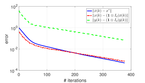
Figure 1: Geometric Rate of Convergence

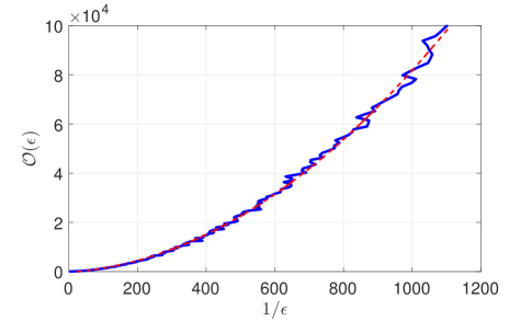
Figure 2: Empirical oracle complexity and its quadratic fitting

We then compare Algorithm 1, abbreviated as D-VSS-SGT, with the distributed stochastic gradient descent (D-SGD) [16] and the distributed stochastic gradient tracking (D-SGT) [23]. We set the consant steplength as $\alpha=0.01$ in the three schemes, $N_{k}=\lceil 0.98^{-k}\rceil$ in Algorithm 1, and terminate them when the total number of sampled gradients utilized reaches 3000. The empirical error $\mathbb{E}\left[\left\|\begin{pmatrix}\bar{x}(k)-x^{*}\\ x(k)-(\mathbf{1}\otimes I_{d})\bar{x}(k)\end{pmatrix}\right\|\right]$ of the three algorithms vs the number of sampled gradients is given in Figure 3. It can be seen that the iterates of D-SGD and D-SGT ceased at a neighborhood of the true parameter $x^{*}$, while the iterate generated by Algorithm 1 converges to the true value $x^{*}$ at a faster convergence speed.

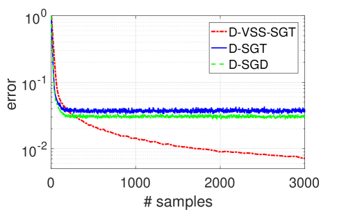
Figure 3: Comparison with D-SGD and D-SGT

V Conclusions

We designed a novel distributed variance reduced stochastic gradient tracking algorithm for strongly convex stochastic optimization over networks. We proved that with a suitably selected constant steplength, the iterates converge in mean to the optimal solution at a geometric rate when the batch-size is increased geometrically. We further establish the complexity bounds for obtaining an $\epsilon$-optimal solution, where the iteration complexity $\mathcal{O}(\ln(1/\epsilon))$ matches the optimal bound of centralized approaches in the deterministic regimes, the communication complexity is significantly reduced to $\mathcal{O}(|\mathcal{N}_{i}|\ln(1/\epsilon))$, and the oracle complexity $\mathcal{O}(1/\epsilon^{2})$ is comparable with the standard stochastic gradient descent algorithm. In future, we will consider asynchronous approaches with agent-specific stepsize and batchsize, and contend with the directed or switching graphs.

In future, we will consider asynchronous approaches with agent-specific stepsize and batchsize, and contend with the directed or switching graphs. It is also worthwhile investigating the communication and oracle complexity for distributed stochastic optimization with other variance reduction methods, like [28],[29] and [30]. The extension of the current algorithm to non-convex/non-smooth distributed stochastic optimization is also a promising research direction.

Appendix A Proof of Lemma 1

Proof of Lemma 1. By multiplying both sides of Eqn. (7a) with ${(\mathbf{1}\otimes I_{d})\over n}$ from the left and using Assumption 1, we obtain that

$$\bar{x}(k+1)=\bar{x}(k)-\alpha\bar{y}(k),\quad\forall k\geq 0.$$ (15)

Also, by using (4b) and Assumption 1, there holds

$$\begin{split}\bar{y}(k+1)&=\bar{y}(k)+{1\over n}\sum_{i=1}^{n}\tilde{g}_{i}(x_{i}(k+1))\\ &\quad-{1\over n}\sum_{i=1}^{n}\tilde{g}_{i}(x_{i}(k)),\quad\forall k\geq 0.\end{split}$$ (16)

Based on Eqn. (16) and the initialization value $y_{i}(0)=\tilde{g}_{i}(x_{i}(0))$, one can recursively show that

$$\bar{y}(k)={1\over n}\sum_{i=1}^{n}\tilde{g}_{i}(x_{i}(k)),\quad\forall k\geq 0.$$ (17)

Step 1: We first give an upper bound on $\|\bar{x}(k+1)-x^{*}\|$. From Eqn. (15), it follows that

$$\|\bar{x}(k+1)-x^{*}\|=\|\bar{x}(k)-\alpha\bar{y}(k)-x^{*}\|$$

$${(a)\atop=}\Big{\|}\bar{x}(k)-x^{*}-{\alpha\over n}\sum_{i=1}^{n}\nabla f_{i}(\bar{x}(k))+{\alpha\over n}\sum_{i=1}^{n}\nabla f_{i}(\bar{x}(k))$$

$$\quad-{\alpha\over n}\sum_{i=1}^{n}\nabla f_{i}(x_{i}(k))+{\alpha\over n}\sum_{i=1}^{n}\nabla f_{i}(x_{i}(k))-\alpha\bar{y}(k)\Big{\|}$$

$${(b)\atop\leq}\left\|\bar{x}(k)-\alpha\nabla F(\bar{x}(k))-x^{*}\right\|$$

$$\quad+{\alpha\over n}\left\|\sum_{i=1}^{n}\nabla f_{i}(\bar{x}(k))-\sum_{i=1}^{n}\nabla f_{i}(x_{i}(k))\right\|$$

$$\quad+\alpha\left\|{1\over n}\sum_{i=1}^{n}\nabla f_{i}(x_{i}(k))-\bar{y}(k)\right\|$$

$${(c)\atop\leq}\left\|\bar{x}(k)-\alpha\nabla F(\bar{x}(k))-x^{*}\right\|+{\alpha\over n}\sum_{i=1}^{n}\left\|w_{i}(k)\right\|$$

$$\quad+{\alpha L\over n}\sum_{i=1}^{n}\|x_{i}(k)-\bar{x}(k)\|,$$ (18)

where in (a) we added and subtracted ${\alpha\over n}\sum_{i=1}^{n}\nabla f_{i}(\bar{x}(k))$ and ${\alpha\over n}\sum_{i=1}^{n}\nabla f_{i}(x_{i}(k))$, in (b) we used the triangle inequality and $F(x)={1\over n}\sum_{i=1}^{n}f_{i}(x)$, and (c) is obtained by using Eqn. (5), Eqn. (17), and Assumption 2(ii). We now introduce an inequality from [31, Eqn. (2.1.24)] on the $\eta$-strongly convex and $L$-smooth function $f(x)$:

$$(x-y)^{T}(\nabla f(x)-\nabla f(y))\geq{\eta L\over\eta+L}\|x-y\|^{2}$$

$$+{1\over\eta+L}\|\nabla f(x)-\nabla f(y)\|^{2},\quad\forall x,y\in\mathbb{R}^{d}.$$ (19)

By $\alpha\in(0,{2\over\eta+L}]$, we have that ${2\over\alpha}-\eta\geq L.$ Define $L^{\prime}\triangleq{2\over\alpha}-\eta$. From Assumption 2 it follows that the function $F(x)={1\over n}\sum_{i=1}^{n}f_{i}(x)$ is $\eta$-strongly convex and $L^{\prime}$-smooth. Thus, by applying Eqn. (A) with $x=x(k)$ and $y=x^{*},$ from $\nabla F(x^{*})=0$ and ${2\over\eta+L^{\prime}}=\alpha$ it follows that

$$\begin{array}[]{ll}&\left\|\bar{x}(k)-\alpha\nabla F(\bar{x}(k))-x^{*}\right\|^{2}\\ &=\left\|\bar{x}(k)-x^{*}\right\|^{2}+\alpha^{2}\left\|\nabla F(\bar{x}(k))\right\|^{2}\\ &-2\alpha(\bar{x}(k)-x^{*})^{T}(\nabla F(\bar{x}(k))-\nabla F(x^{*}))\\ &\leq\left\|\bar{x}(k)-x^{*}\right\|^{2}+\alpha^{2}\left\|\nabla F(\bar{x}(k))\right\|^{2}\\ &-2\alpha\left({\eta L^{\prime}\over\eta+L^{\prime}}\|x_{k}-x^{*}\|^{2}+{1\over\eta+L^{\prime}}\|\nabla F(x_{k})\|^{2}\right)\\ &\leq\Big{(}1-{2\alpha\eta L^{\prime}\over\eta+L^{\prime}}\Big{)}\left\|\bar{x}(k)-x^{*}\right\|^{2}\\ &-\alpha\Big{(}{2\over\eta+L^{\prime}}-\alpha\Big{)}\|\nabla F(x_{k})\|^{2}\\ &\leq\left(1-{2\alpha\eta L^{\prime}\over\eta+L^{\prime}}\right)\left\|\bar{x}(k)-x^{*}\right\|^{2}\\ &=\left(1-\alpha^{2}\eta L^{\prime}\right)\left\|\bar{x}(k)-x^{*}\right\|^{2}=\left(1-\alpha\eta\right)^{2}\left\|\bar{x}(k)-x^{*}\right\|^{2}.\end{array}$$

Then we can bound the first term of Eqn. (A) by

$$\left\|\bar{x}(k)-\alpha\nabla F(\bar{x}(k))-x^{*}\right\|\leq\theta\left\|\bar{x}(k)-x^{*}\right\|$$ (20)

with $\theta\triangleq 1-\alpha\eta.$ Therefore, by plugging Eqn. (20) into Eqn. (A) and using the following relation

$$\sum_{i=1}^{n}\|e_{i}\|_{2}\leq\sqrt{n}\|(e_{1}^{T},\cdots,e_{n}^{T})^{T}\|_{2},$$ (21)

we make further modifications to Eqn. (A) as follows:

$$\|\bar{x}(k+1)-x^{*}\|\leq\theta\|\bar{x}(k)-x^{*}\|$$

$$+\alpha{L\over\sqrt{n}}\|x(k)-(\mathbf{1}\otimes I_{d})\bar{x}(k)\|+{\alpha\over n}\sum_{i=1}^{n}\left\|w_{i}(k)\right\|.$$ (22)

Step 2: We give a bound on $\|x(k+1)-(\mathbf{1}\otimes I_{d})\bar{x}(k+1)\|.$ Because $A\mathbf{1}=\mathbf{1}$ and the spectral radius $\sigma_{A}$ of $A-\mathbf{1}\mathbf{1}^{T}/n$ satisfies $\sigma_{A}\in(0,1),$ for any $x\in\mathbb{R}^{nd}$ we have,

$$\begin{split}&\|(A\otimes I_{d})x-(\mathbf{1}\otimes I_{d})\bar{x}\|\\ &=\|(A-\mathbf{1}\mathbf{1}^{T}/n)\otimes I_{d}\big{(}x-(\mathbf{1}\otimes I_{d})\bar{x}\big{)}\|\\ &\leq\|A-\mathbf{1}\mathbf{1}^{T}/n\|\|x-(\mathbf{1}\otimes I_{d})\bar{x}\|\\ &\leq\sigma_{A}\|x-(\mathbf{1}\otimes I_{d})\bar{x}\|,\end{split}$$ (23)

where $\bar{x}={1\over n}\sum_{i=1}^{n}x_{i}$. This combined with (7a), (15), and the triangle inequality produces the following

$$\begin{array}[]{ll}&\|x(k+1)-(\mathbf{1}\otimes I_{d})\bar{x}(k+1)\|\\ &=\|(A\otimes I_{d})x(k)-\alpha y(k)-(\mathbf{1}\otimes I_{d})(\bar{x}(k)-\alpha\bar{y}(k))\|\\ &\leq\|(A\otimes I_{d})x(k)-(\mathbf{1}\otimes I_{d})\bar{x}(k)\|\\ &+\|\alpha y(k)-\alpha(\mathbf{1}\otimes I_{d})\bar{y}(k)\|\\ &\leq\sigma_{A}\|x(k)-(\mathbf{1}\otimes I_{d})\bar{x}(k)\|+\alpha\|y(k)-(\mathbf{1}\otimes I_{d})\bar{y}(k)\|.\end{array}$$ (24)

Step 3: We give a bound on $\|y(k)-(\mathbf{1}\otimes I_{d})\bar{y}(k)\|$. From Eqns. (5), (6), and (16) it follows that

$$\begin{array}[]{ll}&\bar{y}(k+1)-\bar{y}(k)={1\over n}\sum_{i=1}^{n}\big{(}w_{i}(k+1)+\nabla f_{i}(x_{i}(k+1))\big{)}\\ &-{1\over n}\sum_{i=1}^{n}\big{(}w_{i}(k)+\nabla f_{i}(x_{i}(k))\big{)}\\ &=\left({1\over n}\mathbf{1}^{T}\otimes I_{d}\right)\big{(}\nabla(k+1)+w(k+1)-\nabla(k)-w(k)\big{)}.\end{array}$$

Then by using (7b), (23), $\left\|I_{n}-{1\over n}\mathbf{1}\mathbf{1}^{T}\right\|\leq 1$, and the triangle inequality, we may obtain the following:

$$\|y(k+1)-(\mathbf{1}\otimes I_{d})\bar{y}(k+1)\|$$

$$=\big{\|}(A\otimes I_{d})y(k)+\nabla(k+1)+w(k+1)-\nabla(k)-w(k)$$

$$-(\mathbf{1}\otimes I_{d})\bar{y}(k)+(\mathbf{1}\otimes I_{d})(\bar{y}(k)-\bar{y}(k+1))\big{\|}$$

$$\leq\|(A\otimes I_{d})y(k)-(\mathbf{1}\otimes I_{d})\bar{y}(k)\|+$$

$$\big{\|}\big{(}I_{n}-{1\over n}\mathbf{1}\mathbf{1}^{T}\big{)}\otimes I_{d}(\nabla(k+1)+w(k+1)-\nabla(k)-w(k))\big{\|}$$

$$\leq\sigma_{A}\|y(k)-(\mathbf{1}\otimes I_{d})\bar{y}(k)\|+$$

$$\big{\|}I_{n}-{1\over n}\mathbf{1}\mathbf{1}^{T}\big{\|}\big{(}\|\nabla(k+1)-\nabla(k)\|+\|w(k+1)-w(k)\|\big{)}$$

$$\leq\sigma_{A}\|y(k)-(\mathbf{1}\otimes I_{d})\bar{y}(k)\|$$

$$+L\|x(k+1)-x(k)\|+\|w(k+1)-w(k)\|,$$ (25)

where in the last inequality we used the Lipschitz continuity of $\nabla f_{i}$ (Assumption 2(ii)) and the definition of $\nabla(k)$ in (5).

$$\|\nabla(k+1)-\nabla(k)\|$$

$$=\sqrt{\sum_{i=1}^{n}\|\nabla f_{i}(x_{i}(k+1))-\nabla f_{i}(x_{i}(k))\|^{2}}$$

$$\leq\sqrt{\sum_{i=1}^{n}L^{2}\|x_{i}(k+1)-x_{i}(k)\|^{2}}=L\|x(k+1)-x(k)\|.$$

We then give an estimate for the upper bound of $\|x(k+1)-x(k)\|.$ From (7a) and $A\mathbf{1}=\mathbf{1}$ it follows that

$$\|x(k+1)-x(k)\|=\|(A\otimes I_{d})x(k)-\alpha y(k)-x(k)\|$$

$$=\|(A-I_{n})\otimes I_{d}\big{(}x(k)-(\mathbf{1}\otimes I_{d})\bar{x}(k)\big{)}$$

$$-\alpha\big{(}y(k)-(\mathbf{1}\otimes I_{d})\bar{y}(k)\big{)}-\alpha(\mathbf{1}\otimes I_{d})\bar{y}(k)\|$$

$$\leq\|A-I_{n}\|\big{\|}x(k)-(\mathbf{1}\otimes I_{d})\bar{x}(k)\big{\|}$$

$$+\alpha\|y(k)-(\mathbf{1}\otimes I_{d})\bar{y}(k)\|+\alpha\sqrt{n}\|\bar{y}(k)\|,$$ (26)

where in the last inequality we used the triangle inequality and $\|(\mathbf{1}\otimes I_{d})\bar{y}(k)\|=\sqrt{n}\|\bar{y}(k)\|.$ Then by substituting Eqn. (26) into Eqn. (A) there holds

$$\begin{array}[]{ll}&\|y(k+1)-(\mathbf{1}\otimes I_{d})\bar{y}(k+1)\|\\ &\leq(\sigma_{A}+\alpha L)\|y(k)-(\mathbf{1}\otimes I_{d})\bar{y}(k)\|\\ &+L\|A-I_{n}\|\big{\|}x(k)-(\mathbf{1}\otimes I_{d})\bar{x}(k)\big{\|}\\ &+\alpha\sqrt{n}L\|\bar{y}(k)\|+\|w(k+1)-w(k)\|.\end{array}$$ (27)

Next, we provide an upper bound on $\|\bar{y}(k)\|.$ By using $\sum_{i=1}^{n}\nabla f_{i}(x^{*})=0,$ Eqns. (5) and (17), we obtain that

$$\|\bar{y}(k)\|=\big{\|}{1\over n}\sum_{i=1}^{n}(w_{i}(k)+\nabla f_{i}(x_{i}(k)))\big{\|}$$

$$\leq\big{\|}{1\over n}\sum_{i=1}^{n}w_{i}(k)\big{\|}+\big{\|}{1\over n}\sum_{i=1}^{n}(\nabla f_{i}(x_{i}(k))-\nabla f_{i}(x^{*}))\big{\|}$$

$${(a)\atop\leq}{1\over n}\sum_{i=1}^{n}\left\|w_{i}(k)\right\|+{L\over n}\sum_{i=1}^{n}\|x_{i}(k)-x^{*}\|$$

$${(b)\atop\leq}{1\over n}\sum_{i=1}^{n}\left\|w_{i}(k)\right\|+{L\over\sqrt{n}}\|x(k)-(\mathbf{1}\otimes I_{d})x^{*}\|$$

$${(c)\atop\leq}{1\over n}\sum_{i=1}^{n}\left\|w_{i}(k)\right\|+{L\over\sqrt{n}}\|x(k)-(\mathbf{1}\otimes I_{d})\bar{x}(k)\|$$

$$\quad+{L\over\sqrt{n}}\|(\mathbf{1}\otimes I_{d})\bar{x}(k)-(\mathbf{1}\otimes I_{d})x^{*}\|$$

$$\leq{1\over n}\sum_{i=1}^{n}\left\|w_{i}(k)\right\|+{L\over\sqrt{n}}\|x(k)-(\mathbf{1}\otimes I_{d})\bar{x}(k)\|$$

$$\quad+L\|\bar{x}(k)-x^{*}\|,$$

where in (a) we used Assumption 2(ii), in (b) we utilized Eqn. (21), and in (c) we added and subtracted the term $(\mathbf{1}\otimes I_{d})\bar{x}(k)$ and applied the triangle inequality. This combined with (27) produces

$$\|y(k+1)-(\mathbf{1}\otimes I_{d})\bar{y}(k+1)\|$$

$$\leq(\sigma_{A}+\alpha L)\|y(k)-(\mathbf{1}\otimes I_{d})\bar{y}(k)\|+\alpha\sqrt{n}L^{2}\|\bar{x}(k)-x^{*}\|$$

$$+\left(L\|A-I_{n}\|+\alpha L^{2}\right)\big{\|}x(k)-(\mathbf{1}\otimes I_{d})\bar{x}(k)\big{\|}$$

$$+\|w(k+1)-w(k)\|+{\alpha L\over\sqrt{n}}\sum_{i=1}^{n}\left\|w_{i}(k)\right\|.$$ (28)

Step 4: Obtain a system of inequalities. By the definition of $z(k)$ as in (9), and by combining Eqns. (22), (24), and (A), we obtain that

$$z(k+1) \leq\begin{pmatrix}\theta&\alpha{L\over\sqrt{n}}&0\\ 0&\sigma_{A}&\alpha\\ \alpha\sqrt{n}L^{2}&L\|A-I_{n}\|+\alpha L^{2}&\sigma_{A}+\alpha L\end{pmatrix}z(k)$$

$$+\begin{pmatrix}{\alpha\over n}\sum_{i=1}^{n}\left\|w_{i}(k)\right\|\\ 0\\ \|w(k+1)-w(k)\|+{\alpha L\over\sqrt{n}}\sum_{i=1}^{n}\left\|w_{i}(k)\right\|\end{pmatrix}.$$

Then by recalling $\theta=1-\alpha L$, we prove the lemma. $\Box$

References

- [1] Z. J. Towfic and A. H. Sayed, “Stability and performance limits of adaptive primal-dual networks,” IEEE Transactions on Signal Processing, vol. 63, no. 11, pp. 2888–2903, 2015.
- [2] M. Rabbat and R. Nowak, “Distributed optimization in sensor networks,” in Proceedings of the 3rd international symposium on Information processing in sensor networks. ACM, 2004, pp. 20–27.
- [3] P. Yi, Y. Hong, and F. Liu, “Initialization-free distributed algorithms for optimal resource allocation with feasibility constraints and application to economic dispatch of power systems,” Automatica, vol. 74, pp. 259–269, 2016.
- [4] W. Yu, C. Li, X. Yu, G. Wen, and J. Lü, “Economic power dispatch in smart grids: a framework for distributed optimization and consensus dynamics,” Science China Information Sciences, vol. 61, no. 1, p. 012204, 2018.
- [5] H. Fang, C. Shang, and J. Chen, “An optimization-based shared control framework with applications in multi-robot systems,” Science China Information Sciences, vol. 61, no. 1, p. 014201, 2018.
- [6] Y. Wang, P. Lin, and Y. Hong, “Distributed regression estimation with incomplete data in multi-agent networks,” Science China Information Sciences, vol. 61, no. 9, p. 092202, 2018.
- [7] M. Abdelatti, C. Yuan, W. Zeng, and C. Wang, “Cooperative deterministic learning control for a group of homogeneous nonlinear uncertain robot manipulators,” Science China Information Sciences, vol. 61, no. 11, p. 112201, 2018.
- [8] A. Nedic and A. Ozdaglar, “Distributed subgradient methods for multi-agent optimization,” IEEE Transactions on Automatic Control, vol. 54, no. 1, p. 48, 2009.
- [9] S. Pu, W. Shi, J. Xu, and A. Nedić, “A push-pull gradient method for distributed optimization in networks,” in 2018 IEEE Conference on Decision and Control (CDC). IEEE, 2018, pp. 3385–3390.
- [10] D. P. Palomar and M. Chiang, “A tutorial on decomposition methods for network utility maximization,” IEEE Journal on Selected Areas in Communications, vol. 24, no. 8, pp. 1439–1451, 2006.
- [11] J. F. Mota, J. M. Xavier, P. M. Aguiar, and M. Püschel, “D-admm: A communication-efficient distributed algorithm for separable optimization,” IEEE Transactions on Signal Processing, vol. 61, no. 10, pp. 2718–2723, 2013.
- [12] T.-H. Chang, A. Nedić, and A. Scaglione, “Distributed constrained optimization by consensus-based primal-dual perturbation method,” IEEE Transactions on Automatic Control, vol. 59, no. 6, pp. 1524–1538, 2014.
- [13] P. Yi, Y. Hong, and F. Liu, “Distributed gradient algorithm for constrained optimization with application to load sharing in power systems,” Systems & Control Letters, vol. 83, pp. 45–52, 2015.
- [14] J. Lei, H.-F. Chen, and H.-T. Fang, “Primal–dual algorithm for distributed constrained optimization,” Systems & Control Letters, vol. 96, pp. 110–117, 2016.
- [15] T. Yang, X. Yi, J. Wu, Y. Yuan, D. Wu, Z. Meng, Y. Hong, H. Wang, Z. Lin, and K. H. Johansson, “A survey of distributed optimization,” Annual Reviews in Control, 2019.
- [16] S. S. Ram, A. Nedić, and V. V. Veeravalli, “Distributed stochastic subgradient projection algorithms for convex optimization,” Journal of optimization theory and applications, vol. 147, no. 3, pp. 516–545, 2010.
- [17] K. Srivastava and A. Nedic, “Distributed asynchronous constrained stochastic optimization,” IEEE Journal of Selected Topics in Signal Processing, vol. 5, no. 4, pp. 772–790, 2011.
- [18] J. Lei, H.-F. Chen, and H.-T. Fang, “Asymptotic properties of primal-dual algorithm for distributed stochastic optimization over random networks with imperfect communications,” SIAM Journal on Control and Optimization, vol. 56, no. 3, pp. 2159–2188, 2018.
- [19] D. Jakovetic, D. Bajovic, A. K. Sahu, and S. Kar, “Convergence rates for distributed stochastic optimization over random networks,” in 2018 IEEE Conference on Decision and Control (CDC). IEEE, 2018, pp. 4238–4245.
- [20] D. Yuan, Y. Hong, D. W. Ho, and G. Jiang, “Optimal distributed stochastic mirror descent for strongly convex optimization,” Automatica, vol. 90, pp. 196–203, 2018.
- [21] M. O. Sayin, N. D. Vanli, S. S. Kozat, and T. Başar, “Stochastic subgradient algorithms for strongly convex optimization over distributed networks,” IEEE Transactions on network science and engineering, vol. 4, no. 4, pp. 248–260, 2017.
- [22] A. Nedić and A. Olshevsky, “Stochastic gradient-push for strongly convex functions on time-varying directed graphs,” IEEE Transactions on Automatic Control, vol. 61, no. 12, pp. 3936–3947, 2016.
- [23] S. Pu and A. Nedić, “A distributed stochastic gradient tracking method,” in 2018 IEEE Conference on Decision and Control (CDC). IEEE, 2018, pp. 963–968.
- [24] L. Xiao and S. Boyd, “Fast linear iterations for distributed averaging,” Systems & Control Letters, vol. 53, no. 1, pp. 65–78, 2004.
- [25] R. Xin and U. A. Khan, “A linear algorithm for optimization over directed graphs with geometric convergence,” IEEE Control Systems Letters, vol. 2, no. 3, pp. 315–320, 2018.
- [26] A. Nedich, A. Olshevsky, and W. Shi, “Achieving geometric convergence for distributed optimization over time-varying graphs,” SIAM Journal on Optimization, vol. 27, no. 4, pp. 2597–2633, 2017.
- [27] A. H. Sayed, “Adaptive networks,” Proceedings of the IEEE, vol. 102, no. 4, pp. 460–497, 2014.
- [28] R. Johnson and T. Zhang, “Accelerating stochastic gradient descent using predictive variance reduction,” in Advances in neural information processing systems, 2013, pp. 315–323.
- [29] A. Defazio, F. Bach, and S. Lacoste-Julien, “Saga: A fast incremental gradient method with support for non-strongly convex composite objectives,” in Advances in neural information processing systems, 2014, pp. 1646–1654.
- [30] N. L. Roux, M. Schmidt, and F. R. Bach, “A stochastic gradient method with an exponential convergence _rate for finite training sets,” in Advances in neural information processing systems, 2012, pp. 2663–2671.
- [31] Y. Nesterov, Introductory lectures on convex optimization: A basic course. Springer Science & Business Media, 2013, vol. 87.