TUM-HEP-1250/20
SI-HEP-2019-17
QFET-2019-12
February 7, 2020

Two-loop non-leptonic penguin amplitude
in QCD factorization

Guido Bell^a, Martin Beneke^b, Tobias Huber^a and Xin-Qiang Li^c

^aTheoretische Physik 1, Naturwissenschaftlich-Technische Fakultät,
Universität Siegen, Walter-Flex-Strasse 3, D-57068 Siegen, Germany
^bPhysik Department T31, James-Franck-Straße 1,
Technische Universität München, D–85748 Garching, Germany
^cInstitute of Particle Physics and
Key Laboratory of Quark and Lepton Physics (MOE),
Central China Normal University, Wuhan, Hubei 430079, P. R. China

We complete the calculation of the QCD penguin amplitude at next-to-next-to-leading order in the QCD factorization approach to non-leptonic $B$-meson decays. This provides the last missing piece in the computation of the QCD correction to direct CP asymmetries at leading power in the heavy-quark expansion.

1 Introduction

Direct CP violation arises from the interference of amplitudes with different CP-violating (CKM) and rescattering phases. The values of the CKM parameters in the Standard Model (SM) imply that direct CP violating asymmetries are either very small or require the measurement of rare decays. In $B$-meson physics, rare decays to charmless final states provide the best opportunity to study such CP violation, when there is an interference of an amplitude generated primarily by a tree-level $W$-boson mediated process and a loop-induced $b\to Dg^{*}\,(\to q\bar{q})$ ($D=d,s$) amplitude, called the QCD penguin amplitude.

The theoretical calculation of direct CP asymmetries is very challenging, since it is usually not possible to calculate the rescattering phases in a process involving hadrons. The best prospects are offered by charmless decays to two (pseudoscalar or vector) mesons, in which case the QCD factorization approach [1, 2, 3] provides a rigorous and systematic approximation to the non-leptonic decay amplitudes for the leading term in the heavy quark expansion. The matrix element of the effective Hamiltonian operators $Q_{i}$ (to be specified below) responsible for the $B\to M_{1}M_{2}$ decay can be expressed as

$$\langle M_{1}M_{2}|Q_{i}|\bar{B}\rangle = i\,\frac{m_{B}^{2}}{4}\,\bigg{\{}F^{BM_{1}}(0)\int_{0}^{1}\!du\;T_{i}^{I}(u)\,f_{M_{2}}\phi_{M_{2}}(u)+(M_{1}\leftrightarrow M_{2})$$ (1.1)

$$+\,\int_{0}^{\infty}\!d\omega\int_{0}^{1}\!dudv\;T_{i}^{II}(\omega,v,u)\,f_{B}\phi_{B}(\omega)\;f_{M_{1}}\phi_{M_{1}}(v)\;f_{M_{2}}\phi_{M_{2}}(u)\bigg{\}}$$

in terms of non-perturbative $B\to M$ form factors $F^{BM}(0)$, light-cone distribution amplitudes (LCDAs) $f_{M}\phi_{M}(u)$, and perturbatively calculable hard-scattering kernels $T_{i}^{I}(u)$, $T_{i}^{II}(\omega,v,u)$. Importantly, the rescattering phases are present only in the latter, hence direct CP violation can be calculated once the form factors and LCDAs are known. It also follows that direct CP asymmetries are either of ${\cal O}(\alpha_{s})$, since phases arise from loop contributions to the kernels above, or of next-to-leading power $\mathcal{O}(\Lambda/m_{b})$, where $\Lambda\ll m_{b}$ denotes the strong interaction scale, in the heavy-quark expansion. Since both parameters are $\mathcal{O}(1/10)$ it is a priori unclear whether the direct CP asymmetries in charmless decays are short- or long-distance dominated.

The calculation of the short-distance direct CP asymmetry has therefore been of long-standing interest. The first non-vanishing ${\cal O}(\alpha_{s})$ contribution has been known for a long time from the first QCD factorization calculations [1, 3, 7]. As usual, the next term in the $\alpha_{s}$ expansion is needed to check the reliability of the expansion and to reduce theoretical scale uncertainties. In the present case of direct CP asymmetries, this implies the next-to-next-to-leading order (NNLO) $\mathcal{O}(\alpha_{s}^{2})$ correction to both interfering amplitudes. The $\mathcal{O}(\alpha_{s}^{2})$ correction to the spectator-scattering kernels $T_{i}^{II}(\omega,v,u)$ is somewhat simpler to compute, since it is a one-loop effect, and has been obtained in [8, 9, 10] and [11] for the tree and the QCD and electroweak penguin amplitudes, respectively. The NNLO calculation of the kernel $T_{i}^{I}(u)$ of the form-factor term in (1.1) has been performed about ten years ago [12, 13, 5] for the tree-induced amplitudes $T$, $C$, but only a partial result is currently available for the QCD penguin amplitude, $P$, from 1) the one-loop matrix element of the chromomagnetic dipole operator $Q_{8g}$ [14], and 2) the two-loop matrix elements of the current-current operators $Q_{1,2}^{p}$ [6].

In the present paper we present the calculation of the last missing, and most difficult piece of the NNLO computation, the matrix elements of the penguin operators $Q_{3-6}$ in the effective weak Hamiltonian. Two-loop vertex and two-loop penguin diagrams contribute to these matrix elements, which we compute by extending previous results from [13, 5, 15, 6]. The NNLO computation of the penguin amplitudes provides the basis for a comprehensive reanalysis of the phenomenology of all 130 final states of two pseudoscalar and/or vector mesons from the ground-state nonet [7, 16]. This analysis is deferred to a separate study, while here we present only a numerical result of the penguin amplitude, that puts the new NNLO contribution into perspective.

The paper is organized as follows. In section 2 we lay out the theoretical framework and formulate the problem as a matching calculation of the matrix elements of operators from the effective weak Hamiltonian to a certain four-quark operator in soft-collinear effective theory (SCET), which factorizes into the product of the $B\to M$ form factor and the LCDA of the light meson at the matrix-element level. Section 3 provides some technical details of the two-loop computations in QCD and SCET, and the structure of the result for the hard-scattering kernel before and after the convolution with the Gegenbauer expansion of the light-meson LCDA. The numerical size of the NNLO correction and the residual renormalization scale dependence of the full QCD penguin amplitude is evaluated in section 4. We conclude in section 5. Two appendices summarize the renormalization constants for the operators from the effective weak Hamiltonian required for this work, and list numerical tables from which the convoluted kernels used in section 4 can be reconstructed, including their dependence on the internal charm-quark mass.

2 Theoretical framework

2.1 Penguin amplitude in QCD factorization

On the fundamental level, what is commonly called the QCD penguin amplitude in non-leptonic decays is generated by the loop-induced weak-interaction process $b\to Dg^{*}$, where $D$ refers to a down or strange quark, followed by $g^{*}\to\sum_{q=u,d,s}q\bar{q}$, where the $q$ and $\bar{q}$ end up in different mesons in the final state. This basic process defined by the quark flavour configuration can be dressed by quark and gluon loops.

Following the notation introduced in [7], the charmless two-body decay matrix element of the effective weak Hamiltonian can be decomposed in terms of CKM structures $\lambda_{p}^{(D)}=V_{pD}^{*}V_{pb}$ and flavour operators as

$$\langle M_{1}^{\prime}M_{2}^{\prime}|{\cal H}_{\rm eff}|\bar{B}\rangle=\sum_{p=u,c}\lambda_{p}^{(D)}\,\langle M_{1}^{\prime}M_{2}^{\prime}|{\cal T}_{A}^{p}+{\cal T}_{B}^{p}|\bar{B}\rangle\,.$$ (2.1)

The term ${\cal T}_{A}^{p}$ accounts for the flavour topologies of the form-factor and spectator-scattering terms in (1.1), and ${\cal T}_{B}^{p}$ is reserved for the $1/m_{b}$ suppressed weak annihilation amplitudes. The QCD penguin amplitude corresponds to

$${\cal T}_{A}^{p}\supset\alpha_{4}^{p}(M_{1}M_{2})\,\sum_{q=u,d,s}A([\bar{q}_{s}q][\bar{q}D])\,,$$ (2.2)

where $\bar{q}_{s}$ denotes the spectator anti-quark in the $\bar{B}$ meson. The coefficient $\alpha_{4}^{p}(M_{1}M_{2})$ contains the dynamical information, while the arguments of $A$ encode the flavour composition of the final state $M_{1}M_{2}$ and hence determine the final states $M_{1}^{\prime}M_{2}^{\prime}$ to which the QCD penguin amplitude can contribute.

The matrix element of ${\cal T}_{A}^{p}$ contains kinematical factors as well as the form factors and decay constants that appear in (1.1), as defined in [7, 16], such that $\alpha_{4}^{p}(M_{1}M_{2})$ is a dimensionless number composed of the Wilson coefficients $C_{i}$ of the operators $Q_{i}$ and the convolutions of the hard-scattering kernels with the meson LCDAs. In the QCD factorization approach $\alpha_{4}^{p}(M_{1}M_{2})$ is further divided into the quantities $a_{4}^{p}$, $a_{6}^{p}$,

$$\alpha_{4}^{p}(M_{1}M_{2})=a_{4}^{p}(M_{1}M_{2})\pm r_{\chi}^{M_{2}}a_{6}^{p}(M_{1}M_{2})$$ (2.3)

where the plus (minus) sign applies to the decays where $M_{1}$ is a pseudoscalar (vector) meson. We focus on $a_{4}^{p}(M_{1}M_{2})$ in this paper, which is the only leading-power contribution in the heavy-quark expansion. The normalization of $a_{4}^{p}(M_{1}M_{2})$ is such that

$$a_{4}^{p}=\frac{1}{3}C_{3}+\frac{4}{9}C_{4}+\frac{16}{3}C_{5}+\frac{64}{9}C_{6}+\mathcal{O}(\alpha_{s})\,,\qquad p=u,c$$ (2.4)

in terms of the Wilson coefficients of the effective weak Hamiltonian given in the following subsection. We note that at tree-level $a_{4}^{p}(M_{1}M_{2})$ is independent of the final state and real. However, in higher orders in $\alpha_{s}$, the QCD penguin coefficient in QCD factorization depends on the identity of the final-state mesons through their LCDAs and acquires an imaginary part from loop corrections to the hard-scattering kernels. In the following we describe the calculation of and provide results for the $\mathcal{O}(\alpha_{s}^{2})$ correction to $a_{4}^{p}(M_{1}M_{2})$.

2.2 Operator bases

The calculation is done in the framework of the effective weak Hamiltonian for $b\to D$ transitions, which is given by

$$\mathcal{H}_{\text{eff}}=\frac{4G_{F}}{\sqrt{2}}\;\sum_{p=u,c}V_{pD}^{*}V_{pb}\,\bigg{(}C_{1}Q_{1}^{p}+C_{2}Q_{2}^{p}+\sum_{i=3}^{10}C_{i}Q_{i}+C_{7\gamma}Q_{7\gamma}+C_{8g}Q_{8g}\bigg{)}+\text{h.c.}$$ (2.5)

We adopt the CMM operator basis [17], where the current-current and QCD penguin operators are defined as

$$Q_{1}^{p} =(\bar{p}_{L}\gamma^{\mu}T^{A}b_{L})\;(\bar{D}_{L}\gamma_{\mu}T^{A}p_{L}),$$

$$Q_{2}^{p} =(\bar{p}_{L}\gamma^{\mu}b_{L})\;(\bar{D}_{L}\gamma_{\mu}p_{L}),$$

$$Q_{3} =(\bar{D}_{L}\gamma^{\mu}b_{L})\;{\textstyle\sum_{q}}\;(\bar{q}\gamma_{\mu}q),$$

$$Q_{4} =(\bar{D}_{L}\gamma^{\mu}T^{A}b_{L})\;{\textstyle\sum_{q}}\;(\bar{q}\gamma_{\mu}T^{A}q),$$

$$Q_{5} =(\bar{D}_{L}\gamma^{\mu}\gamma^{\nu}\gamma^{\rho}b_{L})\;{\textstyle\sum_{q}}\;(\bar{q}\gamma_{\mu}\gamma_{\nu}\gamma_{\rho}q),$$

$$Q_{6} =(\bar{D}_{L}\gamma^{\mu}\gamma^{\nu}\gamma^{\rho}T^{A}b_{L})\;{\textstyle\sum_{q}}\;(\bar{q}\gamma_{\mu}\gamma_{\nu}\gamma_{\rho}T^{A}q)\,.$$ (2.6)

Here the sums run over the five quark flavours $q=u$, $d$, $s$, $c$, $b$. The electroweak penguin operators $Q_{7-10}$ and the electromagnetic dipole operator $Q_{7\gamma}$ are irrelevant for the QCD penguin amplitude. Our definition of the chromomagnetic dipole operator,

$$Q_{8g} =\frac{-g_{s}}{32\pi^{2}}\,\overline{m}_{b}\;\bar{D}\sigma_{\mu\nu}(1+\gamma_{5})G^{\mu\nu}b,$$ (2.7)

corresponds to the sign convention $iD_{\mu}=i\partial_{\mu}+g_{s}A^{A}_{\mu}T^{A}$, and $\overline{m}_{b}$ denotes the bottom quark mass in the $\overline{\rm MS}$ scheme at the scale $\mu$.

In dimensional regularization the operator basis has to be supplemented by a set of evanescent operators. In the CMM basis the one-loop evanescent operators are defined as

$$E_{1}^{(1),p} =(\bar{p}_{L}\gamma^{\mu_{1}}\gamma^{\mu_{2}}\gamma^{\mu_{3}}T^{A}b_{L})\;(\bar{D}_{L}\gamma_{\mu_{1}}\gamma_{\mu_{2}}\gamma_{\mu_{3}}T^{A}p_{L})-16Q_{1}^{p},$$

$$E_{2}^{(1),p} =(\bar{p}_{L}\gamma^{\mu_{1}}\gamma^{\mu_{2}}\gamma^{\mu_{3}}b_{L})\;(\bar{D}_{L}\gamma_{\mu_{1}}\gamma_{\mu_{2}}\gamma_{\mu_{3}}p_{L})-16Q_{2}^{p},$$

$$E_{3}^{(1)} =(\bar{D}_{L}\gamma^{\mu_{1}}\gamma^{\mu_{2}}\gamma^{\mu_{3}}\gamma^{\mu_{4}}\gamma^{\mu_{5}}b_{L})\;{\textstyle\sum_{q}}\;(\bar{q}\gamma_{\mu_{1}}\gamma_{\mu_{2}}\gamma_{\mu_{3}}\gamma_{\mu_{4}}\gamma_{\mu_{5}}q)+64Q_{3}-20Q_{5},$$

$$E_{4}^{(1)} =(\bar{D}_{L}\gamma^{\mu_{1}}\gamma^{\mu_{2}}\gamma^{\mu_{3}}\gamma^{\mu_{4}}\gamma^{\mu_{5}}T^{A}b_{L})\;{\textstyle\sum_{q}}\;(\bar{q}\gamma_{\mu_{1}}\gamma_{\mu_{2}}\gamma_{\mu_{3}}\gamma_{\mu_{4}}\gamma_{\mu_{5}}T^{A}q)+64Q_{4}-20Q_{6}\,.$$ (2.8)

At the two-loop level four more evanescent operators arise, defined as [18]

$$E_{1}^{(2),p} =(\bar{p}_{L}\gamma^{\mu_{1}}\gamma^{\mu_{2}}\gamma^{\mu_{3}}\gamma^{\mu_{4}}\gamma^{\mu_{5}}T^{A}b_{L})\;(\bar{D}_{L}\gamma_{\mu_{1}}\gamma_{\mu_{2}}\gamma_{\mu_{3}}\gamma_{\mu_{4}}\gamma_{\mu_{5}}T^{A}p_{L})-256Q_{1}^{p}-20E^{(1),p}_{1}\,,$$

$$E_{2}^{(2),p} =(\bar{p}_{L}\gamma^{\mu_{1}}\gamma^{\mu_{2}}\gamma^{\mu_{3}}\gamma^{\mu_{4}}\gamma^{\mu_{5}}b_{L})\;(\bar{D}_{L}\gamma_{\mu_{1}}\gamma_{\mu_{2}}\gamma_{\mu_{3}}\gamma_{\mu_{4}}\gamma_{\mu_{5}}p_{L})-256Q_{2}^{p}-20E^{(1),p}_{2}\,,$$

$$E_{3}^{(2)} =(\bar{D}_{L}\gamma^{\mu_{1}}\gamma^{\mu_{2}}\gamma^{\mu_{3}}\gamma^{\mu_{4}}\gamma^{\mu_{5}}\gamma^{\mu_{6}}\gamma^{\mu_{7}}b_{L}){\textstyle\sum_{q}}(\bar{q}\gamma_{\mu_{1}}\gamma_{\mu_{2}}\gamma_{\mu_{3}}\gamma_{\mu_{4}}\gamma_{\mu_{5}}\gamma_{\mu_{6}}\gamma_{\mu_{7}}q)+1280Q_{3}-336Q_{5}\,,$$

$$E_{4}^{(2)} =(\bar{D}_{L}\gamma^{\mu_{1}}\gamma^{\mu_{2}}\gamma^{\mu_{3}}\gamma^{\mu_{4}}\gamma^{\mu_{5}}\gamma^{\mu_{6}}\gamma^{\mu_{7}}T^{A}b_{L}){\textstyle\sum_{q}}(\bar{q}\gamma_{\mu_{1}}\gamma_{\mu_{2}}\gamma_{\mu_{3}}\gamma_{\mu_{4}}\gamma_{\mu_{5}}\gamma_{\mu_{6}}\gamma_{\mu_{7}}T^{A}q)$$

$$\;\;\;\;+1280Q_{4}-336Q_{6}\,.$$ (2.9)

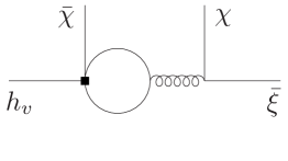
Figure 1: Fermion lines and associated SCET and HQET fields. The black square denotes an insertion of an operator from the effective weak Hamiltonian.

The hard-scattering kernels $T_{i}^{I}(u)$ in (1.1) are determined from matching the QCD matrix elements on the left-hand side of the equation to four-quark operators in SCET. Any four-vector in SCET can be decomposed as

$$p^{\mu} =(n_{+}p)\frac{n_{-}^{\mu}}{2}+(n_{-}p)\frac{n_{+}^{\mu}}{2}+p_{\perp}^{\mu}\,,$$ (2.10)

where the two light-like vectors $n_{\mp}^{\mu}$ which define the collinear and anti-collinear directions, satisfy $n_{-}n_{+}=2$. Eq. (2.10) also defines the perpendicular component. Collinear (anti-collinear) modes have momenta with large component $n_{+}p=\mathcal{O}(m_{b})$ ($n_{-}p=\mathcal{O}(m_{b})$).

We denote the collinear and anti-collinear SCET fields by $\xi$ and $\chi$, respectively, see figure 1. It turns out that there is only one physical SCET operator in our problem. It has the fermion contraction $(\bar{\chi}\chi)(\bar{\xi}h_{v})$ and is given by

$$O_{1} =\sum_{q=u,d,s}(\bar{\chi}_{D}\,\frac{\not{n}_{-}}{2}(1-\gamma_{5})\chi_{q})\;(\bar{\xi}_{q}\,\not{n}_{+}(1-\gamma_{5})h_{v})\,,$$ (2.11)

where $h_{v}$ is the heavy-quark field in heavy-quark effective theory (HQET). In contrast, the diagrams relevant to the penguin amplitude $a_{4}^{p}$ lead to operators where the fermion lines are contracted in a different Fierz ordering, $(\bar{\xi}\chi)(\bar{\chi}h_{v})$, and are therefore of the “wrong-insertion” type (see [5]). The corresponding wrong-insertion SCET operators are conveniently chosen as

$$\widetilde{O}_{n} =\sum_{q=u,d,s}(\bar{\xi}_{q}\,\gamma_{\perp}^{\alpha}\gamma_{\perp}^{\mu_{1}}\gamma_{\perp}^{\mu_{2}}\ldots\gamma_{\perp}^{\mu_{2n-2}}\chi_{q})\;(\bar{\chi}_{D}(1+\gamma_{5})\gamma_{\perp\alpha}\gamma_{\perp\mu_{2n-2}}\gamma_{\perp\mu_{2n-3}}\ldots\gamma_{\perp\mu_{1}}h_{v})\,,$$ (2.12)

where we will need $n$ up to 4 (strings with seven $\gamma$ matrices in each bilinear). The operators $\widetilde{O}_{n}$ are evanescent for $n>1$, while $\widetilde{O}_{1}$ is Fierz-equivalent to $O_{1}/2$ in four dimensions. We therefore add $\widetilde{O}_{1}-O_{1}/2$ as another evanescent operator. In the equations above we omitted the Wilson lines necessary to make the SCET operators, which are non-local on the light-cone [8], gauge-invariant.

2.3 QCD matrix elements

The renormalized matrix element of a QCD operator $Q_{i}$ has the perturbative expansion

$$\langle Q_{i}\rangle = \bigg{\{}\widetilde{A}_{ia}^{(0)}+\frac{\alpha_{s}}{4\pi}\left[\widetilde{A}_{ia}^{(1)}+Z_{ext}^{(1)}\,\widetilde{A}_{ia}^{(0)}+Z_{ij}^{(1)}\widetilde{A}_{ja}^{(0)}\right]$$ (2.13)

$$\hskip 11.38092pt+\,\left(\frac{\alpha_{s}}{4\pi}\right)^{2}\left[\widetilde{A}_{ia}^{(2)}+Z_{ij}^{(1)}\widetilde{A}_{ja}^{(1)}+Z_{ij}^{(2)}\widetilde{A}_{ja}^{(0)}+Z_{ext}^{(1)}\,\widetilde{A}_{ia}^{(1)}+Z_{ext}^{(2)}\,\widetilde{A}_{ia}^{(0)}\right.$$

$$\hskip 11.38092pt\left.+\,Z_{ext}^{(1)}\,Z_{ij}^{(1)}\widetilde{A}_{ja}^{(0)}+Z_{\alpha}^{(1)}\widetilde{A}_{ia}^{(1)}+\,(-i)\,\delta m^{(1)}\,\widetilde{A}^{\prime(1)}_{ia}\right]+{\cal O}(\alpha_{s}^{3})\bigg{\}}\,\langle\widetilde{O}_{a}\rangle^{(0)}\,.$$

Throughout the paper, $\alpha_{s}\equiv\alpha_{s}(\mu)$ denotes the five-flavour strong coupling in the $\overline{\rm MS}$ scheme. Moreover, a superscript on any quantity $G$ labels the order in $\alpha_{s}$ according to

$$G = G^{(0)}+\frac{\alpha_{s}}{4\pi}\,G^{(1)}+\left(\frac{\alpha_{s}}{4\pi}\right)^{2}\,G^{(2)}+{\cal O}(\alpha_{s}^{3})\,.$$ (2.14)

The $\widetilde{A}_{ia}^{(\ell)}$ in (2.13) denote bare $\ell$-loop on-shell matrix elements of QCD operators. For $\ell=2$ we only need matrix elements of the physical operators, but for $\ell<2$ the tree-level and one-loop matrix elements of evanescent operators are required in addition since in terms such as $Z_{ij}^{(1)}\widetilde{A}_{ja}^{(1)}$ the sum over $j$ includes the evanescent operators. For the matching procedure it turns out to be convenient to split up the amplitudes $\widetilde{A}_{ia}^{(\ell)}$ further into factorizable and non-factorizable diagrams, see figure 2,

$$\widetilde{A}_{ia}^{(\ell)} = \widetilde{A}_{ia}^{(\ell){\rm f}}+\widetilde{A}_{ia}^{(\ell){\rm nf}}\,.$$ (2.15)

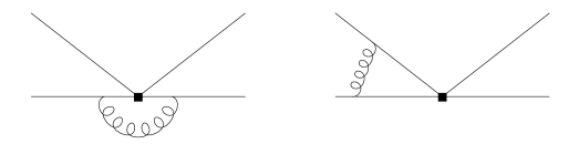
Figure 2: Examples of factorizable (left panel) and non-factorizable (right panel) diagrams.

The renormalization factors $Z_{ij}$, $Z_{\alpha}$, $\delta m$, and $Z_{ext}$ account for operator, coupling, mass, and wave-function renormalization, respectively. The coupling is renormalized in the $\overline{{\rm MS}}$ scheme, whereas the mass and the fields are renormalized in the on-shell scheme. In the matrices $Z_{ij}$ the row index runs over $i=\{Q_{1}^{p},Q_{2}^{p},Q_{3-6},Q_{8g}\}$, while the column index $j$ labels $\{Q_{1}^{p},Q_{2}^{p},Q_{3-6},Q_{8g},E_{1}^{(1),p},E_{2}^{(1),p},E_{3}^{(1)},E_{4}^{(1)},E_{1}^{(2),p},E_{2}^{(2),p},E_{3}^{(2)},E_{4}^{(2)}\}$. They were computed in [19, 18] but need to be adjusted to our operator basis. We give the matrices $Z_{ij}$ explicitly in appendix A.

2.4 SCET matrix elements and hard-scattering kernels

On the SCET side the matrix elements of $\widetilde{O}_{a}$ have a simpler structure. Once dimensional regularization is used as infrared regulator the on-shell renormalization constants are equal to unity, and the bare matrix elements $\widetilde{M}_{ab}^{(\ell)}$ are non-zero only for $\ell>1$. At two loops, only the diagrams with a massive charm quark-loop insertion into the gluon line contribute. Moreover, there is no mass counterterm for a HQET quark. One therefore obtains

$$\langle\widetilde{O}_{a}\rangle = \left\{\delta_{ab}+\frac{\hat{\alpha}_{s}}{4\pi}\,\widetilde{Y}_{ab}^{(1)}+\left(\frac{\hat{\alpha}_{s}}{4\pi}\right)^{\!2}\left[\widetilde{M}_{ab}^{(2)}+\widetilde{Y}_{ab}^{(2)}\right]+{\cal O}(\hat{\alpha}_{s}^{3})\right\}\,\langle\widetilde{O}_{b}\rangle^{(0)}\,.$$ (2.16)

Here $\hat{\alpha}_{s}$ denotes the strong coupling in the four-flavour theory. Since the non-local SCET operators depend on a variable, the renormalization factors $\widetilde{Y}_{ab}=\widetilde{Y}_{ab}(u,u^{\prime})$ are functions of two variables and the product in (2.16) has to be interpreted as a convolution. In the procedure of determining the ultraviolet operator renormalization factors $\widetilde{Y}_{ab}$ one has to regulate infrared divergences other than dimensionally. While the physical operator $O_{1}$ is minimally subtracted in the $\overline{\rm MS}$ scheme, the evanescent operators are renormalized such that their matrix elements with a non-dimensional infrared regulator vanish, so that eventually after renormalization and matching they can be dropped in the evaluation of a physical decay amplitude. Once the $\widetilde{Y}_{ab}$ are at hand, one can use (2.16) with dimensional regularization as infrared and ultraviolet regulator for the on-shell matrix elements of the $\widetilde{O}_{a}$.

The hard-scattering kernels $\widetilde{T}_{i}$ of the operators $Q_{i}$, $i=\{1p,2p,\text{3--6},8g\}$ are then extracted by matching the QCD operators onto SCET,

$$\langle Q_{i}\rangle=\sum\limits_{a}\,\widetilde{H}_{ia}\,\langle\widetilde{O}_{a}\rangle\,,$$ (2.17)

whose steps are explained in detail in [5] and shall not be repeated here. At the end of this procedure we obtain a master formula for the expansion of the wrong-insertion hard-scattering kernels, which is a generalization of the master formula given in [5] to the case when the tree-level matching of the $Q_{i}$ involves evanescent SCET operators. For the tree, one-loop and two-loop kernels, we obtain

$$\frac{1}{2}\,\widetilde{T}_{i}^{(0)} = \widetilde{A}^{(0)}_{i1}\,,$$ (2.18)

$$\frac{1}{2}\,\widetilde{T}_{i}^{(1)} = \widetilde{A}^{(1){\rm nf}}_{i1}+Z_{ij}^{(1)}\,\widetilde{A}^{(0)}_{j1}+\underbrace{\widetilde{A}^{(1){\rm f}}_{i1}-A^{(1){\rm f}}_{31}\,\widetilde{A}^{(0)}_{i1}}_{{\cal{O}}(\epsilon)}-\underbrace{[\widetilde{Y}_{11}^{(1)}-Y_{11}^{(1)}]\,\widetilde{A}^{(0)}_{i1}}_{{\cal{O}}(\epsilon)}-\underbrace{\sum_{b>1}\widetilde{A}_{ib}^{(0)}\,\widetilde{Y}_{b1}^{(1)}}_{{\cal{O}}(\epsilon)}\,,\quad\qquad$$ (2.19)

$$\frac{1}{2}\,\widetilde{T}_{i}^{(2)} = \widetilde{A}^{(2){\rm nf}}_{i1}+Z_{ij}^{(1)}\,\widetilde{A}^{(1)}_{j1}+Z_{ij}^{(2)}\,\widetilde{A}^{(0)}_{j1}+Z_{\alpha}^{(1)}\,\widetilde{A}^{(1){\rm nf}}_{i1}$$ (2.20)

$$+\,(-i)\,\delta m^{(1)}\,\widetilde{A}^{\prime(1){\rm nf}}_{i1}+Z_{ext}^{(1)}\,\big{[}\widetilde{A}^{(1){\rm nf}}_{i1}+Z_{ij}^{(1)}\,\widetilde{A}^{(0)}_{j1}\big{]}$$

$$-\,\frac{1}{2}\,\widetilde{T}_{i}^{(1)}\big{[}C_{FF}^{(1)}+\widetilde{Y}_{11}^{(1)}\big{]}-\sum_{b>1}\widetilde{H}_{ib}^{(1)}\,\widetilde{Y}_{b1}^{(1)}$$

$$+\,[\widetilde{A}^{(2){\rm f}}_{i1}-A^{(2){\rm f}}_{31}\,\widetilde{A}^{(0)}_{i1}]+\,(-i)\,\delta m^{(1)}\,[\widetilde{A}^{\prime(1){\rm f}}_{i1}-A^{\prime(1){\rm f}}_{31}\,\widetilde{A}^{(0)}_{i1}]$$

$$+\,(Z_{\alpha}^{(1)}+Z_{ext}^{(1)})\,[\widetilde{A}^{(1){\rm f}}_{i1}-A^{(1){\rm f}}_{31}\,\widetilde{A}^{(0)}_{i1}]$$

$$-\,[\widetilde{M}^{(2)}_{11}-M^{(2)}_{11}]\,\widetilde{A}^{(0)}_{i1}$$

$$-\,(C_{FF}^{(1)}-\xi_{45}^{(1)})\,[\widetilde{Y}_{11}^{(1)}-Y_{11}^{(1)}]\,\widetilde{A}^{(0)}_{i1}-[\widetilde{Y}_{11}^{(2)}-Y_{11}^{(2)}]\,\widetilde{A}^{(0)}_{i1}$$

$$-\,\sum_{b>1}\widetilde{A}_{ib}^{(0)}\,\widetilde{M}_{b1}^{(2)}-\,\sum_{b>1}\widetilde{A}_{ib}^{(0)}\,\widetilde{Y}_{b1}^{(2)}\,.$$

The factor $1/2$ on the left-hand side appears, since quantities such as $\widetilde{A}^{(n)}_{i1}$ are defined as the coefficients of $\widetilde{O}_{1}$, which after renormalization is replaced by $O_{1}/2$. Together with a factor of 4 from extracting the factor 1/4 in (1.1) this implies $\widetilde{T}_{i}^{(0)}=2\widetilde{A}^{(0)}_{i1}$ etc.

To arrive at (2.20) we traded the four-flavour coupling for the five-flavour one by means of the $D$-dimensional relation $\hat{\alpha}_{s}=\xi_{45}^{-1}\alpha_{s}$, where $\xi_{45}=1+\mathcal{O}(\alpha_{s})$ is given explicitly in [20]. The matching coefficient $C_{FF}$ can be determined from matching calculations for the $b\to u$ transition [21, 22, 20, 23] and reads ($L=\ln(\mu^{2}/m_{b}^{2})$)

$$C_{FF} = 1-\frac{\alpha_{s}}{4\pi}\,\frac{C_{F}}{12}\left(6L^{2}+30L+\pi^{2}+72\right)+{\cal O}(\alpha_{s}^{2})\,.$$ (2.21)

The terms $A^{(\ell){\rm f}}_{31}$ denote $\ell$-loop factorizable matrix elements of $Q_{3}$ of the right-insertion type [5], whose result is proportional to the tree-level matrix element of the physical SCET operator $O_{1}$.

All except three terms in (2.18) – (2.20) have an analogue in the wrong-insertion master formula for the tree amplitudes, which was discussed at length in [5]. The last term in (2.19) and the last line in (2.20) are new. They stem from tree-level matrix elements of the $Q_{i}$ proportional to evanescent SCET operators, convoluted with SCET matrix elements and renormalization constants that describe the mixing of evanescent with physical SCET operators. Such non-vanishing tree-level SCET evanescent operator contributions can appear whenever the operator in $\mathcal{H}_{\text{eff}}$ contains a fermion bilinear with more than one Dirac matrix as is the case for $Q_{5,6}$ and the evanescent QCD operators in (2.8), (2.9).

3 NNLO calculation

3.1 Operator insertions and diagrams

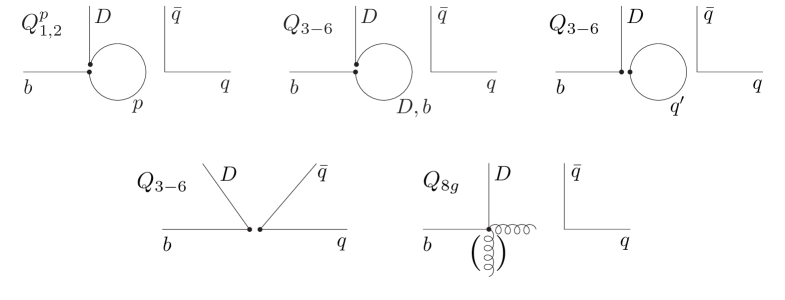
Figure 3: Graphical illustration of the various operator insertions. The symbols stand for $p\in\{u,c\}$, $D\in\{d,s\}$, $q\in\{u,d,s\}$ and $q^{\prime}\in\{u,d,s,c,b\}$. The black dots denote the operator insertion from the effective weak Hamiltonian. Disconnected parts are understood to be connected by gluons.

Several insertions of the operators from the effective weak Hamiltonian contribute to the computation of the penguin amplitudes at higher orders. They are depicted in figure 3. Whereas the current-current operators $Q_{1,2}^{p}$ can be inserted in a single manner only (see first panel of figure 3), there exist several ways of inserting the QCD penguin operators $Q_{3-6}$. Besides the “penguin-type” contractions in the second and third panel of figure 3, also insertions into the “tree-type” diagrams have to be considered, see the lower left panel of figure 3. Finally, there is the insertion of $Q_{8g}$ whose contribution at a given order in $\alpha_{s}$ involves one loop less compared to the other operators. For the counterterm contribution of the master formulas (2.18) – (2.20) also insertions of evanescent QCD operators are required, which are not shown in the figure. Keeping track of all these insertions leads to quite some bookkeeping during the calculation.

The leading order (LO) and next-to-leading order (NLO) contributions to the QCD penguin amplitudes have been known since long [1, 3, 7]. Also the calculation of the NNLO $\mathcal{O}(\alpha_{s}^{2})$ correction involving one-loop spectator scattering dates back more than a decade [11]. The first NNLO calculation of a vertex correction to the leading QCD penguin amplitudes was the one-loop $\mathcal{O}(\alpha_{s}^{2})$ insertion of the chromomagnetic dipole operator $Q_{8g}$ [14]. More recently the current-current operator contribution has been completed [6], and in the present work we compute the remaining insertions from figure 3 at NNLO.

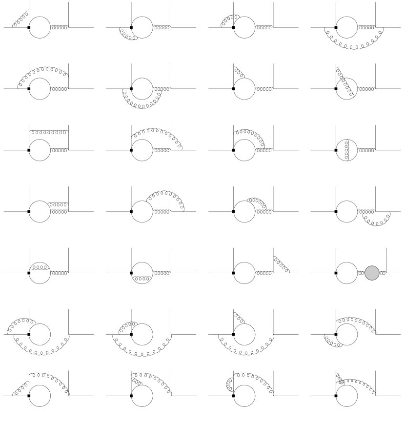
Figure 4: Two-loop penguin diagrams I.

There are in total more than a hundred diagrams that one has to compute at NNLO. Those of the “penguin-type” contractions are shown in figures 4 and 5. We found after explicit calculation that the sum of all diagrams in figure 5 vanishes for all operator insertions. In addition, one has to insert the QCD penguin operators $Q_{3-6}$ into the “tree-type” diagrams which are shown explicitly in section 5 of [2]. Finally, the one-loop diagrams for the chromomagnetic dipole operator $Q_{8g}$ are depicted in figure 6.

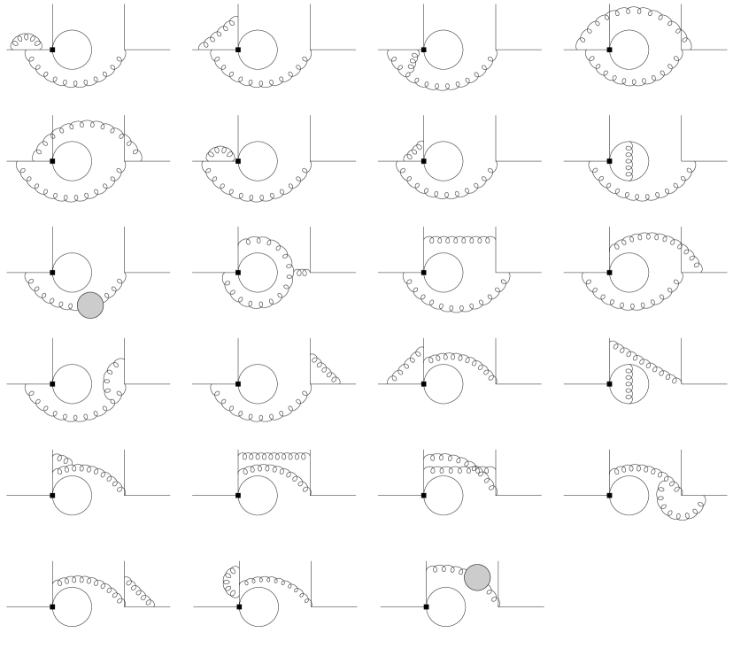
Figure 5: Two-loop penguin diagrams II. The sum of these diagrams vanishes for all operator insertions.

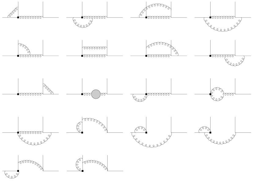
Figure 6: One-loop diagrams of the chromomagnetic dipole operator $Q_{8g}$.

3.2 Details of the two-loop calculation

To obtain the vertex kernels $T_{i}^{I}(u)$ the quark matrix elements $\langle D(uq)\bar{q}(\bar{u}q)q(p)|Q_{i}|b(p_{b})\rangle$ must be calculated at the two-loop order. Some general kinematic features can be seen from the one-loop penguin contraction:

The light quark flavours are taken to be massless and therefore the particle in the fermion loop (solid circle) can have mass $m_{f}=0$ (light quarks), $m_{f}=m_{c}$ (charm quark) or $m_{f}=m_{b}$ (bottom quark). The external states are on-shell and satisfy $p_{b}^{2}=m_{b}^{2}$ and $p^{2}=q^{2}=0$. The quark that goes into meson $M_{2}$ carries momentum fraction $u\in[0,1]$ of $q$, the anti-quark the remaining fraction $\bar{u}\equiv 1-u$. There is a kinematic threshold at $\bar{u}=4m_{c}^{2}/m_{b}^{2}$ in the charm-loop diagrams.

The problem at hand is a genuine two-scale problem with dimensionless quantities $\bar{u}$ and $z_{f}=(m_{f}^{2}-i\eta)/m_{b}^{2}$, where the infinitesimally small quantity $\eta>0$ determines the sign of the analytic continuation. For later convenience we also define the following additional kinematic variables [15]

$$r =\sqrt{1-4z_{c}}\,, s =\sqrt{1-4z_{c}/\bar{u}}\,,$$

$$s_{1} =\sqrt{1-4z_{b}/\bar{u}}\,, s_{u} =\sqrt{1-4z_{c}/u}\,,$$

$$s_{u,1} =\sqrt{1-4z_{b}/u}\,,$$

$$v =\frac{1+s_{1}}{2}+\frac{1-s_{1}}{2}\sqrt{1+\frac{8(1+s_{1})z_{c}}{(1-s_{1})^{2}}}\,, t =\frac{1-s_{1}}{2}+\frac{1+s_{1}}{2}\sqrt{1+\frac{8(1-s_{1})z_{c}}{(1+s_{1})^{2}}}\,,$$

$$v_{0} =\frac{1-i\sqrt{3}}{2}\,r+\frac{1+i\sqrt{3}}{2}=v(u=0)\,, t_{0} =\frac{1+i\sqrt{3}}{2}\,r+\frac{1-i\sqrt{3}}{2}=t(u=0)\,,$$

$$p =\frac{1-\sqrt{u^{2}+4\bar{u}z_{c}}}{\bar{u}}\,, p_{u} =\frac{1-\sqrt{\bar{u}^{2}+4uz_{c}}}{u}\,.$$ (3.1)

The methods that we apply in the two-loop calculation have become standard in contemporary advanced multi-loop computations. We work in dimensional regularization with $D=4-2\epsilon$, where ultraviolet and infrared (soft and collinear) divergences appear as poles in $\epsilon$. We first apply a Passarino – Veltman [24] reduction to the tensor structure of the amplitude. The Dirac and colour algebra is then performed by means of in-house routines. Subsequently, the dimensionally regularized scalar integrals are reduced to master integrals using the Laporta algorithm [25, 26] based on integration-by-parts (IBP) identities [27, 28]. To this end we use the package FIRE [29] and an in-house routine. The master integrals that stem from the insertion of penguin operators into the “tree-type” diagrams are known analytically since long [12, 13, 30, 5] and evaluate to harmonic polylogarithms (HPLs) [31]. Those that come from the reduction of the diagrams in figures 4 and 5 were computed analytically in [15] in terms of iterated integrals over generalized weight functions.

In the notation of [15] the generalized HPLs are defined as

$$H_{\vec{0}_{n}}(x) =\frac{1}{n!}\ln^{n}(x)\,,$$

$$H_{a_{1},a_{2},\ldots,a_{n}}(x) =\int_{0}^{x}dt\;f_{a_{1}}(t)\,H_{a_{2},\ldots,a_{n}}(t)\,.$$ (3.2)

For the weight functions we have $f_{0}(x)=1/x$, while for any expression with $w\neq 0$ we define

$${f_{w}(x)=\frac{1}{w-x}}\,,\qquad{f_{-w}(x)=\frac{1}{w+x}}\,.$$ (3.3)

Moreover it turns out to be convenient to define the linear combinations

$$f_{w^{+}}(x)= f_{w}(x)+f_{-w}(x)=\frac{2w}{w^{2}-x^{2}}\,,$$

$$f_{w^{-}}(x)= f_{w}(x)-f_{-w}(x)=\frac{2x}{w^{2}-x^{2}}\,.$$ (3.4)

In our calculation, we encounter the following expressions for $w$,

$$w_{1}= \,1\,, w_{4} =1+\sqrt{1-r^{2}}\,, w_{6} ={w_{2}}_{\big{|}z_{c}\to z_{b}}\,,$$

$$w_{2}= \,r\,, w_{5} =1-\sqrt{1-r^{2}}\,, w_{7} ={w_{4}}_{\big{|}z_{c}\to z_{b}}\,,$$

$$w_{3}= \,\frac{r^{2}+1}{2}\,.$$ (3.5)

Finally there is one new master integral that stems from the one-loop diagrams in figure 6, whose analytic result reads

$$\int\!\frac{d^{D}k}{(2\pi)^{D}}\,\frac{u}{\left[k^{2}\right]\,\left[(k+uq)^{2}-m_{b}^{2}\right]\,\left[(k+p_{b})^{2}-m_{b}^{2}\right]}$$ (3.6)

$$=-(iS_{\Gamma})\,(m_{b}^{2})^{-1-\epsilon}\,\Gamma(1-\epsilon)\Gamma(1+\epsilon)\left(3H_{w_{1}^{+},w_{1}^{+}}(s_{1})-3i\pi H_{w_{1}^{+}}(s_{1})-8\zeta_{2}+\mathcal{O}(\epsilon)\right)\,,$$

where $S_{\Gamma}=1/((4\pi)^{D/2}\,\Gamma(1-\epsilon))$ and $\zeta_{2}=\pi^{2}/6$.

3.3 Calculation of the counterterms

The diagrams shown in figures 4 – 6 and their calculation discussed in the previous subsection refer to the term $\widetilde{A}^{(2){\rm nf}}_{i1}$ in the expression for $\widetilde{T}_{i}^{(2)}$ in the master formula (2.20). In the following we remark on the remaining terms in (2.20) complementing the discussion of the corresponding terms in [5] for the calculation of the colour-allowed and colour-suppressed tree amplitudes.

We begin with the terms on the right-hand side of the expression (2.19) for the one-loop kernels $\widetilde{T}_{i}^{(1)}$. The first term, $Z_{ij}^{(1)}\,\widetilde{A}^{(0)}_{j1}$, following the bare non-factorizable one-loop amplitudes $\widetilde{A}^{(1){\rm nf}}_{i1}$, is the counterterm that renormalizes the operator $Q_{i}$. The implicit sum over $j$ includes the evanescent operators in the effective weak Hamiltonian. The next term, $\widetilde{A}^{(1){\rm f}}_{i1}-A^{(1){\rm f}}_{31}\,\widetilde{A}^{(0)}_{i1}$ arises, because the factorizable one-loop terms that are not part of the kernels but of the full QCD form factors correspond to right insertions of $Q_{3}$, while the fermion lines of the $Q_{i}$ are contracted in the wrong-insertion order for the QCD penguin amplitude. The difference must be put into $\widetilde{T}_{i}^{(1)}$ to reproduce the full amplitude. However, it turns out to be ${\cal{O}}(\epsilon)$ and can therefore be dropped in the limit $\epsilon\to 0$. The last two terms in (2.19) appear, because the matrix elements of the evanescent SCET operators $\widetilde{O}_{1}-O_{1}/2$, $\widetilde{O}_{b}$ with $b>1$ with a non-dimensional infrared regulator must be renormalized to zero. The non-minimal one-loop renormalization factors $\widetilde{Y}_{11}^{(1)},\widetilde{Y}_{b1}^{(1)}$ may give finite contributions to the kernels. Once again we find that these contributions actually vanish as $\epsilon\to 0$. However, this no longer holds true at the two-loop order.

The counter- and subtraction terms needed to obtain finite two-loop hard-scattering kernels $\widetilde{T}_{i}^{(2)}$ in (2.20) are much more involved. The first two lines of (2.20) represent ultraviolet counterterms for the operators $Q_{i}$, including external field as well as bottom and charm mass renormalization. The internal quark masses are taken to be the pole masses, hence $\delta m^{(1)}$ is the counterterm for the pole mass. There are no internal massive quark lines in the $\mathcal{O}(\alpha_{s})$ matrix element of the chromomagnetic dipole operator $Q_{8g}$. However, the mass parameter $\overline{m}_{b}$ that appears in the definition (2.7) of the operator is understood to be the $\overline{\rm MS}$ mass and the mass counterterm is not included in the anomalous dimension matrix from [18]. The conversion to the pole mass then implies that the same counterterm $\delta m^{(1)}$ is applied multiplicatively to the bare amplitude $\widetilde{A}^{(1){\rm nf}}_{8g1}$.

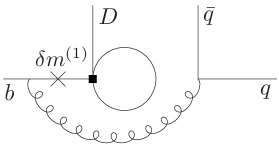
Figure 7: Non-vanishing tadpole contribution to $(-i)\,\delta m^{(1)}\,\widetilde{A}^{\prime(1){\rm nf}}_{i1}$, $i=3,\ldots,6$.

It is interesting to note that $(-i)\,\delta m^{(1)}\,\widetilde{A}^{\prime(1){\rm nf}}_{i1}$ is the only place where fermion-tadpole contractions of the four-quark operators survive in the counterterms. The relevant diagram is shown in figure 7. For the one-loop tadpole diagrams without the mass counterterm insertion there is a cancellation between the two diagrams obtained from attaching the gluon to the external fermion lines to the left and above the four-quark vertex. This cancellation does not occur for the mass counterterm tadpole diagram, since it only exists for the massive $b$-quark line. The non-vanishing tadpole contribution is divergent and required to make the final result for $\widetilde{T}_{i}^{(2)}$ finite. The corresponding tadpole contribution vanishes for the $Q_{1,2}^{p}$ matrix elements due to the $(V-A)\otimes(V-A)$ structure of these operators. In the bare two-loop matrix elements almost all the tadpole contractions cancel (see figure 5), and only two diagrams give a net contribution (see last line of figure 4).

The remaining terms on the right-hand side of the two-loop master formula (2.20) represent generalizations of similar structures in (2.19) and account for i) the use of the full QCD rather than SCET $B\to M$ form factors, ii) the renormalization of the SCET operators, iii) non-vanishing two-loop SCET bare matrix elements due to massive internal charm loops, iv) the finite subtractions required to make the renormalized matrix elements of evanescent operators vanish.

As was the case in the calculation of the topological tree amplitudes, the expression $-\sum_{b>1}\widetilde{H}_{ib}^{(1)}\,\widetilde{Y}_{b1}^{(1)}$ in the third line of (2.20) vanishes in the limit $\epsilon\to 0$. The finite one-loop hard-scattering kernels $\widetilde{H}_{ib}^{(1)}$ are non-zero for $b=2,3$, but the mixing of the evanescent operators into $\widetilde{O}_{1}$, $\widetilde{Y}_{b1}^{(1)}$ turns out to be $\mathcal{O}(\epsilon)$. We recall that the renormalization factors $\widetilde{Y}_{a1}^{(\ell)}$ are functions of two momentum fractions $u^{\prime},u$. Expressions such as $-\sum_{b>1}\widetilde{H}_{ib}^{(1)}\,\widetilde{Y}_{b1}^{(1)}$ therefore represent convolutions in $u^{\prime}$ with the hard-scattering kernels. In case of $\widetilde{T}_{i}^{(1)}\widetilde{Y}_{11}^{(1)}$ in the third line, since $\widetilde{Y}_{11}^{(1)}$ contains a $1/\epsilon^{2}$ singularity, the $D$-dimensional hard-scattering kernel $\widetilde{T}_{i}^{(1)}$ must be expanded to $\mathcal{O}(\epsilon^{2})$. The convolution can then be quite involved.

It is advantageous to rearrange some of the terms in (2.20). To this end, we define the one-loop kernel without the terms from the SCET evanescent operator renormalization,

$$\frac{1}{2}\,\widetilde{T}_{i}^{(1)F}\equiv\widetilde{A}^{(1){\rm nf}}_{i1}+Z_{ij}^{(1)}\,\widetilde{A}^{(0)}_{j1}+\widetilde{A}^{(1){\rm f}}_{i1}-A^{(1){\rm f}}_{31}\,\widetilde{A}^{(0)}_{i1}\,.$$ (3.7)

Notice that $\widetilde{T}_{i}^{(1)F}$ must be computed to $\mathcal{O}(\epsilon^{2})$, since it multiplies the renormalization constant $\widetilde{Y}_{11}^{(1)}$, which contains $1/\epsilon^{2}$ poles. Hence, the term $\widetilde{A}^{(1){\rm f}}_{i1}-A^{(1){\rm f}}_{31}\widetilde{A}^{(0)}_{i1}$, which is $\mathcal{O}(\epsilon)$ cannot be dropped here. We then combine terms in (2.20) as follows:

$$-\frac{1}{2}\,\widetilde{T}_{i}^{(1)}\widetilde{Y}_{11}^{(1)}-[\widetilde{Y}_{11}^{(2)}-Y_{11}^{(2)}]\,\widetilde{A}^{(0)}_{i1}-\sum_{b>1}\widetilde{A}_{ib}^{(0)}\,\widetilde{Y}_{b1}^{(2)}$$ (3.8)

$$= -\frac{1}{2}\,\widetilde{T}_{i}^{(1)F}\widetilde{Y}_{11}^{(1)}+\underbrace{\left\{[\widetilde{Y}_{11}^{(1)}-Y_{11}^{(1)}]\,\widetilde{Y}_{11}^{(1)}-[\widetilde{Y}_{11}^{(2)}-Y_{11}^{(2)}]\right\}\widetilde{A}^{(0)}_{i1}}_{\equiv\,\hat{\Delta}}$$

$$+\,\underbrace{\sum_{b>1}\widetilde{A}_{ib}^{(0)}\,\left(\widetilde{Y}_{b1}^{(1)}\widetilde{Y}_{11}^{(1)}-\widetilde{Y}_{b1}^{(2)}\right)}_{\equiv\,\hat{\mathcal{E}}}\,.$$

The combination of renormalization constants $\hat{\Delta}$ was already computed in [5]. The quantity $\hat{\mathcal{E}}$ appears only for the matrix elements of $Q_{5,6}$, which have non-vanishing tree-level contributions $\widetilde{A}_{ib}^{(0)}$ proportional to the evanescent SCET operator $\widetilde{O}_{2}$. As discussed in [5], the advantage of defining $\hat{\Delta}$, $\hat{\mathcal{E}}$ is that while the individual terms in these expressions depend on the infrared regulator chosen to compute the non-minimal evanescent operator renormalization constants, $\hat{\Delta}$, $\hat{\mathcal{E}}$ are regulator-independent, as indeed the final result must be. By applying infrared rearrangements, in which the product of one-loop renormalization factors appears as subgraph of the two-loop factor, $\hat{\Delta}$, $\hat{\mathcal{E}}$ can be computed directly without the need of ever introducing an explicit infrared regulator.

With these remarks we provide explicit expressions for

$$\widetilde{A}^{(2){\rm f}}_{i1}-A^{(2){\rm f}}_{31}\,\widetilde{A}^{(0)}_{i1}=\left\{1,\frac{4}{3},32,\frac{128}{3}\right\}\,\frac{8}{27}\left(\frac{1}{\epsilon}+2L\right)+\left\{1,\frac{4}{3},32,\frac{128}{3}\right\}\frac{4}{27}n_{0}T_{f}$$

$$\hskip 101.00737pt+\left\{1,\frac{4}{3},64,\frac{256}{3}\right\}\frac{7}{27}\,,\qquad$$ (3.9)

$$(-i)\,\delta m^{(1)}\,[\widetilde{A}^{\prime(1){\rm f}}_{i1}-A^{\prime(1){\rm f}}_{31}\,\widetilde{A}^{(0)}_{i1}]=\mathcal{O}(\epsilon)\,,$$ (3.10)

$$(Z_{\alpha}^{(1)}+Z_{ext}^{(1)})\,[\widetilde{A}^{(1){\rm f}}_{i1}-A^{(1){\rm f}}_{31}\,\widetilde{A}^{(0)}_{i1}]=\left\{1,\frac{4}{3},32,\frac{128}{3}\right\}\left(-\frac{8}{27}n_{f}T_{f}+\frac{26}{9}\right),$$ (3.11)

$$-\,[\widetilde{M}^{(2)}_{11}-M^{(2)}_{11}]\,\widetilde{A}^{(0)}_{i1}=\left\{1,\frac{4}{3},16,\frac{64}{3}\right\}\frac{4}{27}T_{f}\,,$$ (3.12)

$$-\,(C_{FF}^{(1)}-\xi_{45}^{(1)})\,[\widetilde{Y}_{11}^{(1)}-Y_{11}^{(1)}]\,\widetilde{A}^{(0)}_{i1}=\mathcal{O}(\epsilon)\,,$$ (3.13)

$$-\,\sum_{b>1}\widetilde{A}_{ib}^{(0)}\,\widetilde{M}_{b1}^{(2)}=\left\{0,0,1,\frac{4}{3}\right\}\,\frac{64}{27}T_{f}\,,$$ (3.14)

$$\hat{\Delta}=\left\{1,\frac{4}{3},16,\frac{64}{3}\right\}\left(-\frac{4}{27}(n_{0}+1)T_{f}+\frac{17}{27}\right),$$ (3.15)

$$\hat{\mathcal{E}}=\left\{0,0,1,\frac{4}{3}\right\}\left(-\frac{64}{27}(n_{0}+1)T_{f}+\frac{16}{27}\right),$$ (3.16)

which we expanded in $\epsilon$ up to $\mathcal{O}(\epsilon^{0})$. The four entries in curly brackets refer to $i=3,4,5,6$. $L=\ln\frac{\mu^{2}}{m_{b}^{2}}$, $T_{f}=1/2$. $n_{0}=3$ denotes the number of massless flavours, and $n_{f}=5$ the total number of flavours.

3.4 Hard-scattering kernels

Although most of the individual terms in the master formulas (2.18) – (2.20) have poles in the dimensional regulator $\epsilon$, the total expression for the hard-scattering kernels (HSK) $\widetilde{T}_{i}^{(\ell)}$ must be free of poles in $\epsilon$, which we checked analytically to $\mathcal{O}(\alpha_{s}^{2})$ and for all $i\in\{1u,2u,1c,2c,\text{3-6},8g\}$.

The tree-level and one-loop HSK are known from [1]. However, the calculation was performed with another operator basis for the effective weak Hamiltonian [32], which is less suitable for NNLO calculations than the CMM basis [17]. For completeness, we therefore begin by summarizing the tree-level and one-loop HSK in the CMM basis and in the notation of the present paper.

At tree-level the HSK relevant for the penguin amplitude read

$$\widetilde{T}^{(0)}_{1u} =0\,, \widetilde{T}^{(0)}_{2c} =0\,, \widetilde{T}^{(0)}_{5} =16/N_{c}\,,$$

$$\widetilde{T}^{(0)}_{2u} =0\,, \widetilde{T}^{(0)}_{3} =1/N_{c}\,, \widetilde{T}^{(0)}_{6} =16C_{F}/N_{c}\,,$$

$$\widetilde{T}^{(0)}_{1c} =0\,, \widetilde{T}^{(0)}_{4} =C_{F}/N_{c}\,, \widetilde{T}^{(0)}_{8g} =0\,,$$ (3.17)

with $N_{c}=3$ and $C_{F}=(N_{c}^{2}-1)/(2N_{c})=4/3$. At $\mathcal{O}(\alpha_{s})$ the HSK are conveniently expressed in terms of the following functions,

$$G(z_{c},\bar{u}) =\frac{2(12z_{c}+5\bar{u}-3\bar{u}\ln(z_{c}))}{9\bar{u}}-\frac{2s(2z_{c}+\bar{u})}{3\bar{u}}\ln\left(\frac{s+1}{s-1}\right)$$

$$=\frac{2(12z_{c}+5\bar{u}-3\bar{u}\ln(z_{c}))}{9\bar{u}}-\frac{2s(2z_{c}+\bar{u})}{3\bar{u}}\left(H_{w_{1}^{+}}(s)-i\pi\right)\,,$$ (3.18)

$$G(z_{b},\bar{u}) =\frac{2(12+5\bar{u})}{9\bar{u}}-\frac{2s_{1}(2+\bar{u})}{3\bar{u}}\ln\left(\frac{s_{1}+1}{s_{1}-1}\right)$$

$$=\frac{2(12+5\bar{u})}{9\bar{u}}-\frac{2s_{1}(2+\bar{u})}{3\bar{u}}\left(H_{w_{1}^{+}}(s_{1})-i\pi\right)\,,$$ (3.19)

$$G(0,\bar{u}) =-\frac{2}{3}\,\ln(\bar{u})+\frac{2}{3}i\pi+\frac{10}{9}\,,$$ (3.20)

$$t_{1}(u) =-22-3i\pi+3\left(1-\frac{u}{\bar{u}}\right)\ln u$$

$$\quad\,+\bigg{[}2\,{\rm Li}_{2}(u)-\ln^{2}(u)-\left(1+2i\pi-\frac{2u}{\bar{u}}\right)\ln(u)-(u\to\bar{u})\bigg{]}.$$ (3.21)

The variable $s$ is as in (3.1) and also $z_{f}=(m_{f}^{2}-i\eta)/m_{b}^{2}$ is as before. The penguin function $G(z_{f},\bar{u})$ coincides with the corresponding function defined in [3], while $t_{1}(u)$ is related to the one-loop vertex function $g(u)$ in that reference by $t_{1}(u)=g(u)-22$. One then has

$$\widetilde{T}^{(1)}_{1u} =-\frac{C_{F}}{2N_{c}^{2}}\left[-\frac{2}{3}\,L+\frac{2}{3}-G(0,\bar{u})\right]\,, \quad\widetilde{T}^{(1)}_{2u} =-2N_{c}\,\widetilde{T}^{(1)}_{1u}\,,$$

$$\widetilde{T}^{(1)}_{1c} =-\frac{C_{F}}{2N_{c}^{2}}\left[-\frac{2}{3}\,L+\frac{2}{3}-G(z_{c},\bar{u})\right]\,, \quad\widetilde{T}^{(1)}_{2c} =-2N_{c}\,\widetilde{T}^{(1)}_{1c}\,,$$

$$\widetilde{T}^{(1)}_{3} =\frac{C_{F}}{N_{c}}\left[-\frac{22}{3}\,L+t_{1}(u)+\frac{4}{3}-G(0,\bar{u})-G(z_{b},\bar{u})\right]+\widetilde{T}^{(1)}_{8g}\,,$$

$$\widetilde{T}^{(1)}_{4} =-\frac{1}{2N_{c}}\,\widetilde{T}^{(1)}_{3}-C_{F}+\frac{C_{F}}{N_{c}}\left[-\frac{2}{3}\,n_{f}\,L-n_{0}\,G(0,\bar{u})-G(z_{c},\bar{u})-G(z_{b},\bar{u})\right]\,,$$

$$\widetilde{T}^{(1)}_{5} =16\,\widetilde{T}^{(1)}_{3}+\frac{16C_{F}}{3\,N_{c}}+4\,\widetilde{T}^{(1)}_{8g}\,,$$

$$\widetilde{T}^{(1)}_{6} =-\frac{3}{N_{c}}\,\widetilde{T}^{(1)}_{3}+10\,\widetilde{T}^{(1)}_{4}-\frac{2}{N_{c}}\,\widetilde{T}^{(1)}_{8g}-\frac{4C_{F}}{N_{c}}\left(\frac{15}{2}N_{c}+\frac{2}{3N_{c}}-n_{f}\right)\,,$$

$$\widetilde{T}^{(1)}_{8g} =-\frac{2C_{F}}{N_{c}\bar{u}}\,.$$ (3.22)

Note that the HSK must be calculated to higher orders in $\epsilon$ when they enter a term in the master formula at higher loop order, since they usually multiply terms that are divergent in $\epsilon$. We refrain from giving terms beyond $\mathcal{O}(\epsilon^{0})$ here since they are straightforward to derive.

At $\mathcal{O}(\alpha_{s}^{2})$ only the kernel $\widetilde{T}^{(2)}_{8g}$ of the chromomagnetic dipole operator is of a length suitable for printing, and given by the expression

$$\widetilde{T}^{(2)}_{8g} =\frac{8L}{9\bar{u}}+\frac{64}{27\bar{u}}\,L\,\ln(\bar{u})+\frac{8\ln(u)}{27\bar{u}}-\frac{16(\bar{u}-4z_{c})(\bar{u}+2z_{c})}{27\,s\,\bar{u}^{3}}\,(H_{w_{1}^{+}}(s)-i\pi)-\frac{16}{27\bar{u}}\,\text{Li}_{2}(\bar{u})$$

$$-\frac{4(\bar{u}-4)\left(\bar{u}^{3}+5\bar{u}^{2}-12\bar{u}+8\right)}{27s_{1}u^{2}\bar{u}^{3}}\,(H_{w_{1}^{+}}(s_{1})-i\pi)+\frac{8\left(49\bar{u}^{2}-61\bar{u}+24\right)}{81u\bar{u}^{2}}+\frac{64z_{c}}{27\bar{u}^{2}}$$

$$-\frac{8(\bar{u}-2)}{9u^{3}\bar{u}}\,(H_{w_{1}^{+},w_{1}^{+}}(s_{1})-i\pi\,H_{w_{1}^{+}}(s_{1}))-\frac{4\pi^{2}(\bar{u}-3)\left(\bar{u}^{2}-5\right)}{81u^{3}\bar{u}}-\frac{4i\pi\left(3\bar{u}^{2}+\bar{u}+14\right)}{27u^{2}\bar{u}}$$

$$+\frac{4\left(5\bar{u}^{2}-17\bar{u}+30\right)}{27u^{2}\bar{u}}\,\ln(\bar{u})+\frac{4\left(7\bar{u}^{3}-21\bar{u}^{2}+29\bar{u}-6\right)}{27u^{3}\bar{u}}\,\ln^{2}(\bar{u})-\frac{8}{27\bar{u}}\,i\pi\ln(u)$$

$$-\frac{8\left(9\bar{u}^{3}-27\bar{u}^{2}+35\bar{u}-8\right)}{27u^{3}\bar{u}}\,i\pi\ln(\bar{u})-\frac{16\ln(z_{c})}{27\bar{u}}-\frac{4}{27\bar{u}}\,\ln^{2}(u)-\frac{8\ln(\bar{u})\ln(u)}{27\bar{u}}\,,$$ (3.23)

where we substituted numerical values for the colour and flavour factors. The explicit expressions for $H_{w_{1}^{+}}(s)$ and $H_{w_{1}^{+},w_{1}^{+}}(s)$ are

$$H_{w_{1}^{+}}(s) = \ln\left(\frac{1+s}{1-s}\right)=\ln\left(\frac{s+1}{s-1}\right)+i\pi\,,$$ (3.24)

$$H_{w_{1}^{+},w_{1}^{+}}(s) = \frac{1}{2}\,H^{2}_{w_{1}^{+}}(s)\,.$$ (3.25)

The kernel $\widetilde{T}^{(2)}_{8g}$ was previously calculated in [14]. Our expression (3.23) confirms this result. The expressions for the two-loop penguin HSK of the operators $Q_{1,2}^{p},Q_{3-6}$ are long and complicated, although they are available analytically as a linear combination of the generalized HPLs introduced in section 3.2. We provide the analytic expressions for all HSK at $\mathcal{O}(\alpha_{s}^{2})$ electronically as supplementary material to the present article.

3.5 Convolution in Gegenbauer moments

The HSK enter the formula of the QCD penguin amplitudes via the convolution with the LCDA $\phi_{M}(u)$ of the light meson. The LCDA is expanded into the eigenfunctions of the one-loop renormalization kernel,

$$\phi_{M}(u) = 6\,u\,\bar{u}\,\left[1+\sum_{n=1}^{\infty}a_{n}^{M}\,C^{(3/2)}_{n}(2u-1)\right]\,,$$ (3.26)

where $a_{n}^{M}\equiv a_{n}^{M}(\mu)$ and $C^{(3/2)}_{n}(x)$ are the Gegenbauer moments and polynomials, respectively. We truncate the Gegenbauer expansion (3.26) at $n=2$, which is sufficient in practice.

The convolution of those parts of the HSK that come from operator insertions into “tree-type” diagrams is performed in the same way as in [12, 13, 5] and can be done completely analytically. The terms that stem from “penguin-type” diagrams, however, require a different and more refined treatment. A method that is applicable to the majority of the terms is to trade $u$ for $s=\sqrt{1-4z_{c}/\bar{u}}$ as integration variable, which results in $s=r$ and $s=+i\infty$ as integration limits for $s$,

$$\int\limits_{0}^{1}\!du\;\widetilde{T}_{i}(u)\;\phi_{M}(u)=\int\limits_{r}^{+i\infty}\!\!ds\;\frac{2s(r^{2}-1)}{(1-s^{2})^{2}}\,\widetilde{T}_{i}(u(s))\;\phi_{M}(u(s))\,.$$ (3.27)

The threshold at $\bar{u}=4z_{c}$ is mapped to $s=0$. The main advantage of this substitution is the ability to perform the integration over $s$ in terms of the same iterated integrals as in section 3.2. Subtleties arise, however, when taking the limits $s\to r$ and $s\to+i\infty$ of the integral function. In case of the lower limit individual terms contain power divergences proportional to $1/(r-s)^{n}$. They can be isolated via a Taylor expansion about $s=r$ of the corresponding numerators and disappear in the sum of all terms. Taking the upper limit requires an argument inversion of the generalized HPLs. This is done recursively via the following formulas:

$$H_{w^{+},\vec{w}}\left(\frac{1}{y}\right) =H_{w^{+},\vec{w}}(a)-\int\limits_{y}^{\frac{1}{a}}\!dt\;\frac{2\,{\textstyle{\frac{1}{w}}}}{\left({\textstyle{\frac{1}{w}}}\right)^{2}-t^{2}}\,H_{\vec{w}}\left(\frac{1}{t}\right)\,,$$

$$H_{w^{-},\vec{w}}\left(\frac{1}{y}\right) =H_{w^{-},\vec{w}}(a)-\int\limits_{y}^{\frac{1}{a}}\!dt\;\left[\frac{2}{t}+\frac{2\,t}{\left({\textstyle{\frac{1}{w}}}\right)^{2}-t^{2}}\right]\,H_{\vec{w}}\left(\frac{1}{t}\right)\,,$$

$$H_{0,\vec{w}}\left(\frac{1}{y}\right) =H_{0,\vec{w}}(a)+\int\limits_{y}^{\frac{1}{a}}\!dt\;\frac{1}{t}\,H_{\vec{w}}\left(\frac{1}{t}\right)\,.$$ (3.28)

The recursion ends at HPLs of weight one, where the explicit form of the argument inversion can be easily computed, e.g.

$$H_{w_{2}^{-}}\left(\frac{1}{t}\right) =H_{{\textstyle{(\frac{1}{w_{2}})}}^{-}}(t)+2H_{0}(t)+2H_{0}(r)+i\pi\,,$$ (3.29)

which holds for arbitrary values of $1/t$ on the positive, imaginary axis. In this way, logarithmic divergences contained in generalized HPLs as $s\to+i\infty$ are made explicit, as in

$$H_{w_{2}^{-},0}(s) \stackrel{{\scriptstyle s\to+i\infty}}{{\longrightarrow}}-2H_{0,0}(s)+H_{{\textstyle{(\frac{1}{w_{2}})}}^{-},0}(-i)+H_{w_{2}^{-},0}(i)-\frac{\pi^{2}}{4}+\mathcal{O}\left(\frac{1}{s}\right)\,.$$ (3.30)

The divergences that arise in individual terms as $s\to+i\infty$ have to cancel in the end as well. This procedure yields generalized HPLs up to weight five, which we evaluate numerically by means of the program GiNaC [33, 34]. The complex number $a$ in (3.28) is in principle arbitrary. The choice $a=i$ in the argument inversion turns out to be convenient for the numerical evaluation.

There are a few terms to which the above procedure cannot be applied since the dependence on the kinematic variables is more involved, e.g. in products of HPLs of different $u$-dependent arguments. Fortunately, these terms are easy to integrate numerically and/or are free from kinematic thresholds. In the latter case we derive Mellin-Barnes (MB) representations for the integrals and perform the convolution over $u$ analytically. The subsequent integration over the MB variables can be done numerically to high accuracy using MB.m [35].

In this way, we obtain all terms in the leading QCD penguin amplitudes that involve powers of $L=\ln(\mu^{2}/m_{b}^{2})$ completely analytically. In the $L^{0}$ pieces a few terms are obtained only as an interpolation in $z_{c}$. We present all the expressions out of which the penguin amplitudes are built in the next section.

As an independent check we evaluated the convolution integrals for a fixed value of the charm-quark mass numerically, based on a grid of 230 points in $u$ that was designed to capture the singular behavior of the hard-scattering kernels at the endpoints $u\to 0,1$ and at the charm threshold $u=1-4z_{c}$. We then fitted the integrands to a suitable ansatz in the singular regions, while we used interpolating functions in the regions where the integrands are smooth. In this way we compared our results for the convolution integrals for all considered Gegenbauer moments and 25 different values of the charm-quark mass, and found agreement between the two methods at the subpercent level, except for a few outliers that are due to large numerical cancellations.

4 Penguin amplitudes with NNLO accuracy

4.1 Analytic expressions

In the CMM basis the leading QCD penguin amplitudes $a_{4}^{p}$ with $p=u,c$ become, after expanding through to the second Gegenbauer moment,

$$a_{4}^{p}= \;\frac{C_{3}}{N_{c}}+\frac{C_{F}}{N_{c}}C_{4}+\frac{16C_{5}}{N_{c}}+\frac{16C_{F}}{N_{c}}C_{6}$$

$$+\frac{\alpha_{s}}{4\pi}\frac{C_{F}}{N_{c}}\left[\left(C_{3}-\frac{C_{4}}{2N_{c}}+16C_{5}-\frac{8C_{6}}{N_{c}}\right)(-6L+I^{(1)}_{t})\right.$$

$$\qquad\qquad\quad+\left(C_{8g}+C_{3}-\frac{C_{4}}{2\,N_{c}}+20C_{5}-\frac{10\,C_{6}}{N_{c}}\right)(-2)\,I^{(1)}_{8g}$$

$$\qquad\qquad\quad+\left(C_{2}-\frac{C_{1}}{2N_{c}}\right)\left(-\frac{2}{3}\,L+\frac{2}{3}-\delta_{pu}\,I^{(1)}_{0}-\delta_{pc}\,I^{(1)}_{c}\right)$$

$$\qquad\qquad\quad+\left(C_{3}-\frac{C_{4}}{2N_{c}}+16C_{5}-\frac{8C_{6}}{N_{c}}\right)\left(-\frac{4}{3}\,L+\frac{4}{3}-I^{(1)}_{0}-I^{(1)}_{b}\right)$$

$$\qquad\qquad\quad+\Big{(}C_{4}+10C_{6}\Big{)}\left(-\frac{2}{3}\,n_{f}\,L-n_{0}\,I^{(1)}_{0}-I^{(1)}_{c}-I^{(1)}_{b}\right)$$

$$\qquad\qquad\quad\left.-N_{c}C_{4}+\frac{16}{3}C_{5}-4\left(10N_{c}+\frac{2}{3N_{c}}-n_{f}\right)C_{6}\right]$$

$$+\left(\frac{\alpha_{s}}{4\pi}\right)^{2}\bigg{[}C_{1}\left(\delta_{pu}\,I^{(2)}_{1u}+\delta_{pc}\,I^{(2)}_{1c}\right)+C_{2}\left(\delta_{pu}\,I^{(2)}_{2u}+\delta_{pc}\,I^{(2)}_{2c}\right)$$

$$\qquad\qquad\quad+\sum\limits_{i=3}^{6}C_{i}\,I^{(2)}_{i}+C_{8g}\,I^{(2)}_{8g}\bigg{]}\,.$$ (4.1)

As before, we use $L=\ln(\mu^{2}/m_{b}^{2})$ and $z_{f}=(m_{f}^{2}-i\eta)/m_{b}^{2}$. The functions $I^{(1)}_{t,0,c,b,8g}$ denote the convolution of the functions in (3.18) – (3.21) with the Gegenbauer expansion (3.26) of the light-meson LCDA. They are known analytically [3],

$$I^{(1)}_{t} =\int\limits_{0}^{1}\!du\;t_{1}(u)\;\phi_{M}(u)=-\frac{45}{2}-3i\pi+a_{1}^{M}\left(\frac{11}{2}-3i\pi\right)-\frac{21}{20}\,a_{2}^{M}\;,$$ (4.2)

$$I^{(1)}_{0} =\int\limits_{0}^{1}\!du\;G(0,\bar{u})\;\phi_{M}(u)=\frac{5}{3}+\frac{2i\pi}{3}+\frac{1}{2}\,a_{1}^{M}+\frac{1}{5}\,a_{2}^{M}\;,$$ (4.3)

$$I^{(1)}_{c} = \int\limits_{0}^{1}\!du\;G(z_{c},\bar{u})\;\phi_{M}(u)\,=\,\frac{r^{2}+2}{2}\,\left(r^{2}-1\right)^{2}g_{3}(r)-\frac{r}{3}\left(3r^{4}-7r^{2}+6\right)g_{1}(r)-\frac{2}{3}\ln(z_{c})$$ (4.4)

$$\hskip 34.14322pt+\,\frac{1}{3}\left(r^{2}-2\right)\left(3r^{2}-8\right)$$

$$+\,a_{1}^{M}\left[\frac{9}{16}\left(3r^{4}+2r^{2}+3\right)\left(r^{2}-1\right)^{2}g_{3}(r)-\frac{27}{8}r\left(r^{2}+1\right)\!\left(r^{2}-1\right)^{2}\!g_{1}(r)\right.$$

$$\hskip 34.14322pt\left.+\frac{1}{8}\left(27r^{6}-18r^{4}-69r^{2}+64\right)\right]$$

$$+\,a_{2}^{M}\left[\frac{9}{8}\left(5r^{6}+r^{2}+2\right)\left(r^{2}-1\right)^{2}g_{3}(r)-\frac{3}{4}r\left(15r^{4}+5r^{2}+6\right)\left(r^{2}-1\right)^{2}g_{1}(r)\right.$$

$$\hskip 34.14322pt\left.+\frac{1}{20}\left(225r^{8}-300r^{6}+85r^{4}-230r^{2}+224\right)\right]\,,$$

$$I^{(1)}_{b} = \int\limits_{0}^{1}\!du\;G(z_{b},\bar{u})\;\phi_{M}(u)=\frac{85}{3}-6\sqrt{3}\pi+\frac{4\pi^{2}}{9}+a_{1}^{M}\left(-\frac{155}{2}+36\sqrt{3}\pi-12\pi^{2}\right)$$ (4.5)

$$+\,a_{2}^{M}\left(\frac{7001}{5}-504\sqrt{3}\pi+136\pi^{2}\right)\,,$$

$$I^{(1)}_{8g} = \int\limits_{0}^{1}\!du\;\frac{\phi_{M}(u)}{\bar{u}}=3\left(1+a_{1}^{M}+a_{2}^{M}\right)\;,$$ (4.6)

where we used the variable $r=\sqrt{1-4z_{c}}$. The functions $g_{1}(r)$ and $g_{3}(r)$ can be found in (B.2). At $\mathcal{O}(\alpha_{s}^{2})$, all terms involving $L$ were also obtained in a fully analytic manner, while the $L^{0}$ terms are analytic only for $I^{(2)}_{1u}$, $I^{(2)}_{2u}$ and $I^{(2)}_{8g}$. For the $L^{0}$ term in $I^{(2)}_{1c}$, $I^{(2)}_{2c}$ and $I^{(2)}_{3-6}$ we calculated numerical values for several hundred points in the interval $0.01\leq z_{c}\leq 1$. We provide the data tables for these functions electronically in ancillary files, and in this write-up present fits which reproduce the data at the level of $5$ per mille for all $0.01\leq z_{c}\leq 1$. For the physical region $0.05<z_{c}<0.2$ the agreement is well below the per-mille level. All functions that contribute at $\mathcal{O}(\alpha_{s}^{2})$ are collected in appendix B.

4.2 Numerical results

The convoluted kernels and fit coefficient tables allow for a fast evaluation of the two-loop penguin amplitude. In the following we discuss the size of the new correction and present for the first time the numerical value of the complete leading QCD penguin amplitude at NNLO. For the sake of comparison with previous partial results, in particular [6], we adopt the same values for the hadronic parameters as in that reference, which in turn are mostly the same as adopted in [5] for the evaluation of the topological tree amplitudes at NNLO in QCD factorization. The form-factor contribution to $a_{4}^{p}$ depends only on the Gegenbauer moments of the light-meson LCDA. The spectator-scattering contribution further depends on form factors, the $B$-meson decay constant and LCDA, and light-quark masses.

The penguin amplitude coefficients $a_{4}^{u,c}$ depend on the final state mesons through the hadronic parameters. We present the result for the $\pi\bar{K}$ final state:

$$a_{4}^{u}(\pi\bar{K})/10^{-2} = -2.87-[0.09+0.09i]_{\rm V_{1}}+[0.49-1.32i]_{\rm P_{1}}$$ (4.7)

$$-[0.32+0.71i]_{\rm P_{2},\,Q_{1,2}}+[0.33+0.38i]_{\rm P_{2},\,Q_{3-6,8g}}$$

$$+\,\left[\frac{r_{\rm sp}}{0.434}\right]\Big{\{}[0.13]_{\rm LO}+[0.14+0.12i]_{\rm HV}-[0.01-0.05i]_{\rm HP}+[0.07]_{\rm tw3}\Big{\}}$$

$$= (-2.12^{+0.48}_{-0.29})+(-1.56^{+0.29}_{-0.15})i\,,$$

$$a_{4}^{c}(\pi\bar{K})/10^{-2} = -2.87-[0.09+0.09i]_{\rm V_{1}}+[0.05-0.62i]_{\rm P_{1}}$$ (4.8)

$$-[0.77+0.50i]_{\rm P_{2},\,Q_{1,2}}+[0.33+0.38i]_{\rm P_{2},\,Q_{3-6,8g}}$$

$$+\,\left[\frac{r_{\rm sp}}{0.434}\right]\Big{\{}[0.13]_{\rm LO}+[0.14+0.12i]_{\rm HV}+[0.01+0.03i]_{\rm HP}+[0.07]_{\rm tw3}\Big{\}}$$

$$= (-3.00^{+0.45}_{-0.32})+(-0.67^{+0.50}_{-0.39})i\,.$$

In both equations the first two lines originate from the form-factor term (kernels $T_{i}^{I}$ in (1.1)). The third line is the spectator-scattering contribution (kernels $T_{i}^{II}$ in (1.1)), which was computed to $\mathcal{O}(\alpha_{s}^{2})$ in [11]. Spectator scattering has only a small effect on the penguin amplitude for $r_{\rm sp}=0.434$ and we do not discuss it further.

The second line in (4.7), (4.8) represents the NNLO correction to the form-factor term, which is further split into the contribution from the current-current operators $Q_{1,2}^{p}$ and the penguin operators $Q_{3-6,8g}$. The first reproduces the result from [6]. The second, $[0.33+0.38i]_{\rm P_{2},\,Q_{3-6,8g}}$, is the main result of this paper. Note that the penguin operators contribute equally to $a_{4}^{u}$ and $a_{4}^{c}$. Comparing the new correction to the LO (unlabelled) and NLO (labelled V₁ and P₁) contribution, we see that the real part constitutes a $(10-15)\%$ correction relative to LO and is a sizeable fraction of the NLO term. The imaginary part is especially important as it is responsible for the existence of a direct CP asymmetry and vanishes at LO. In case of $a_{4}^{u}(\pi\bar{K})$, the new contribution represents a $-27\%$ correction, and for $a_{4}^{c}(\pi\bar{K})$ it reaches $-54\%$. However, for both, the real and imaginary part there is a strong cancellation between the NNLO correction from the current-current operators $Q_{1,2}^{p}$ and from the penguin operators $Q_{3-6,8g}$, resulting in a much reduced overall NNLO correction.

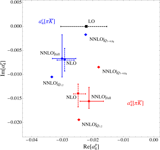
Figure 8: Anatomy of QCD corrections to $a_{4}^{u}$ and $a_{4}^{c}$. The points to the lower right (red in colour) refer to $a_{4}^{u}$, those to the upper left (blue in colour) to $a_{4}^{c}$. The LO point is equal for both. See text for further explanation.

The numerical situation is illustrated in figure 8 in the complex $a_{4}^{p}$ plane, which shows the LO, NLO and NNLO approximation to the QCD penguin amplitude, including the spectator-scattering term. At NNLO, we show in addition the previous result (labelled NNLO$|_{Q_{1,2}}$) from [6] and for comparison the result when the current-current operator rather than the penguin operator contributions to the NNLO form-factor term are excluded (labelled NNLO$|_{Q_{3-6,8g}}$). That the full NNLO result lies between the two previous points illustrates the above mentioned cancellation. Note that the LO and NLO numerical values shown in the figure do not correspond precisely to the values of the LO and NLO terms in (4.7), (4.8). The reason is that in the NNLO result we employ Wilson coefficients $C_{i}$ in the CMM basis evolved to the bottom-quark mass scale with next-to-next-to-leading logarithmic accuracy, while in the NLO (LO) result we use only next-to-leading logarithmic (leading logarithmic) accuracy. Eqs. (4.7), (4.8), on the other hand, represents a split-up of the NNLO expression into terms of different orders in $\alpha_{s}$, but always employing next-to-next-to-leading logarithmic Wilson coefficients. As a consequence the full NNLO result is even closer to the NLO result than the cancellations in (4.7), (4.8) suggest.

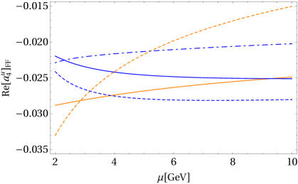
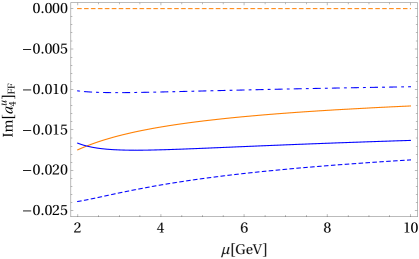
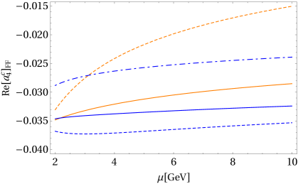
Figure 9: Scale dependence of $a_{4}^{u}(\pi\bar{K})$ (upper row) and $a_{4}^{c}(\pi\bar{K})$ (lower row). The spectator-scattering contribution is not included here. Real part to the left, imaginary part to the right. Line coding: full NNLO (solid, dark-grey/blue), NNLO$|_{Q_{3-6,8g}}$ (dash-dotted, dark-grey/blue), NNLO$|_{Q_{1,2}}$ (dashed, dark-grey/blue), NLO (solid, light-grey/orange), LO (dashed, light-grey/orange).

The natural renormalization scale of the form factor term is the bottom-quark mass scale. In figure 9 we display the residual renormalization scale dependence of the form-factor contribution to $a_{4}^{p}$. The various lines refer to the approximations of figure 8 as explained in the caption, with the solid, dark-grey (blue) line representing the full NNLO result. At this order the scale dependence is negligible, especially for $\mu>4\,$GeV. The last line in (4.7) and (4.8) provides an estimate of the theoretical uncertainty of the entire QCD penguin amplitude coefficient $a_{4}^{p}$, which is also shown in figure 8. Figure 8 also displays the uncertainty at LO and NLO for comparison. Somewhat surprisingly, the uncertainty is larger at NNLO than at NLO. Most of this effect is caused by the NNLO $\mathcal{O}(\alpha_{s}^{2})$ correction to spectator scattering, and hence was present already in [11]. The total uncertainty arises to a large part from the uncertainty in hadronic input parameters, which cannot be reduced by perturbative calculations. The dominant hadronic uncertainties are due to the second Gegenbauer moment of the light-meson LCDAs and, despite the smallness of the spectator-scattering contribution, the inverse moment $\lambda_{B}$ of the $B$-meson LCDA. We note, however, that the two-loop correction to the form-factor term calculated in the present paper roughly doubles the sensitivity to the first two Gegenbauer moments of the light-meson LCDA. Similarly, the sensitivity of $\mbox{Im}\,[a_{4}^{c}]_{\rm FF}$ to the value of the charm-quark mass is larger in the NNLO approximation than at NLO.

5 Conclusion

In this paper we computed the remaining missing piece to the leading QCD penguin amplitude at NNLO in QCD factorization from the two-loop matrix elements of the penguin operators $Q_{3-6}$ in the effective weak Hamiltonian. The new contribution is sizeable and cancels in part the previously known current-current operator contribution. With this result, direct CP asymmetries in charmless $B$ decays, which are largely determined by the interference of the QCD penguin amplitude with the topological tree amplitudes, can for the first time be calculated including the first QCD correction. The Belle II experiment is expected to measure many charmless $B$ decays with unprecedented precision in the near future, motivating a reconsideration of the analysis of complete sets of charmless final states with pseudoscalar and/or vector mesons in the framework of QCD factorization. Such analyses can now be performed with NNLO perturbative calculations.

Acknowledgements

We thank Stefan Weinzierl for useful correspondence on GiNaC and the authors of [14] for correspondence on their result. The work of GB and TH was supported by DFG Forschergruppe FOR 1873 “Quark Flavour Physics and Effective Field Theories”. The work of MB is supported by the DFG Sonderforschungsbereich/Transregio 110 “Symmetries and the Emergence of Structure in QCD”. The work of XL is supported by the National Natural Science Foundation of China under Grant Nos. 11675061 and 11435003, and by the Fundamental Research Funds for the Central Universities under Grant No. CCNU18TS029.

Appendix A Renormalization constants

Here we list the matrices $Z_{ij}$ needed for operator renormalization. The row index runs over $i=\{Q_{1}^{p},Q_{2}^{p},Q_{3-6},Q_{8g}\}$, while the column index $j$ labels

$$\{\underbrace{Q_{1}^{p},Q_{2}^{p}}_{C},\underbrace{Q_{3-6}}_{P},\underbrace{Q_{8g}}_{M},\underbrace{E_{1}^{(1),p},E_{2}^{(1),p},E_{3}^{(1)},E_{4}^{(1)}}_{E^{(1)}},\underbrace{E_{1}^{(2),p},E_{2}^{(2),p},E_{3}^{(2)},E_{4}^{(2)}}_{E^{(2)}}\}\,.$$ (A.1)

The matrices $Z_{ij}$ were computed in [19, 18], but need to be adjusted to our operator basis since our definition of $Q_{8g}$ differs from that in [19, 18]. We split up the matrices into several blocks,

$$Z^{(1)}=\frac{1}{\epsilon}\left(\begin{array}[]{ccccc}(Z^{(1)}_{CC})_{2\times 2}&(Z^{(1)}_{CP})_{2\times 4}&(Z^{(1)}_{CM})_{2\times 1}&(Z^{(1)}_{CE^{(1)}})_{2\times 4}&(Z^{(1)}_{CE^{(2)}})_{2\times 4}\\[5.69054pt] (Z^{(1)}_{PC})_{4\times 2}&(Z^{(1)}_{PP})_{4\times 4}&(Z^{(1)}_{PM})_{4\times 1}&(Z^{(1)}_{PE^{(1)}})_{4\times 4}&(Z^{(1)}_{PE^{(2)}})_{4\times 4}\\[5.69054pt] 0&0&(Z^{(1)}_{MM})_{1\times 1}&0&0\end{array}\right)\,,$$ (A.2)

$$Z^{(2)}=\sum\limits_{k=1}^{2}\frac{1}{\epsilon^{k}}\left(\begin{array}[]{ccccc}(Z^{(2),k}_{CC})_{2\times 2}&(Z^{(2),k}_{CP})_{2\times 4}&(Z^{(2),k}_{CM})_{2\times 1}&(Z^{(2),k}_{CE^{(1)}})_{2\times 4}&(Z^{(2),k}_{CE^{(2)}})_{2\times 4}\\[5.69054pt] (Z^{(2),k}_{PC})_{4\times 2}&(Z^{(2),k}_{PP})_{4\times 4}&(Z^{(2),k}_{PM})_{4\times 1}&(Z^{(2),k}_{PE^{(1)}})_{4\times 4}&(Z^{(2),k}_{PE^{(2)}})_{4\times 4}\\[5.69054pt] 0&0&(Z^{(2),k}_{MM})_{1\times 1}&0&0\end{array}\right)\,,$$ (A.3)

which in our operator basis, for $n_{f}=5$ quark flavours and $T_{f}=1/2$ read

$$Z^{(1)}_{CC} =\left(\begin{array}[]{cc}-2&\frac{4}{3}\\[2.84544pt] 6&0\end{array}\right)\,, Z^{(1)}_{CP} =\left(\begin{array}[]{cccc}0&-\frac{1}{9}&0&0\\[2.84544pt] 0&\frac{2}{3}&0&0\end{array}\right)\,, Z^{(1)}_{CM} =\left(\begin{array}[]{c}\frac{167}{648}\\[2.84544pt] \frac{19}{27}\end{array}\right)\,,$$ (A.10)

$$Z^{(1)}_{CE^{(1)}} =\left(\begin{array}[]{cccc}\frac{5}{12}&\frac{2}{9}&0&0\\[2.84544pt] 1&0&0&0\end{array}\right)\,, Z^{(1)}_{CE^{(2)}} =\left(\begin{array}[]{cccc}0&0&0&0\\[2.84544pt] 0&0&0&0\end{array}\right)\,,$$ (A.15)

$$Z^{(2),1}_{CC} =\left(\begin{array}[]{cc}\frac{317}{36}&-\frac{515}{54}\\[2.84544pt] \frac{349}{12}&3\end{array}\right)\,, Z^{(2),1}_{CP} =\left(\begin{array}[]{cccc}-\frac{353}{243}&-\frac{1567}{972}&\frac{67}{486}&-\frac{35}{648}\\[2.84544pt] -\frac{104}{81}&\frac{338}{81}&\frac{14}{81}&\frac{35}{108}\end{array}\right)\,, Z^{(2),1}_{CM} =\left(\begin{array}[]{c}-\frac{9625}{8748}\\[2.84544pt] \frac{5749}{5832}\end{array}\right)\,,$$ (A.22)

$$Z^{(2),1}_{CE^{(1)}} =\left(\begin{array}[]{cccc}\frac{4493}{864}&-\frac{49}{648}&0&0\\[2.84544pt] \frac{1031}{144}&\frac{8}{9}&0&0\end{array}\right)\,, Z^{(2),1}_{CE^{(2)}} =\left(\begin{array}[]{cccc}\frac{1}{384}&-\frac{35}{864}&0&0\\[2.84544pt] -\frac{35}{192}&-\frac{7}{72}&0&0\end{array}\right)\,,$$ (A.27)

$$Z^{(2),2}_{CC} =\left(\begin{array}[]{cc}\frac{41}{3}&-\frac{58}{9}\\[2.84544pt] -29&4\end{array}\right)\,, Z^{(2),2}_{CP} =\left(\begin{array}[]{cccc}\frac{10}{81}&\frac{209}{162}&-\frac{1}{81}&-\frac{5}{216}\\[2.84544pt] -\frac{20}{27}&-\frac{128}{27}&\frac{2}{27}&\frac{5}{36}\end{array}\right)\,, Z^{(2),2}_{CM} =\left(\begin{array}[]{c}-\frac{28189}{17496}\\[2.84544pt] -\frac{7249}{1458}\end{array}\right)\,,$$ (A.34)

$$Z^{(2),2}_{CE^{(1)}} =\left(\begin{array}[]{cccc}-\frac{125}{36}&-\frac{73}{54}&0&0\\[2.84544pt] -\frac{73}{12}&0&0&0\end{array}\right)\,, Z^{(2),2}_{CE^{(2)}} =\left(\begin{array}[]{cccc}\frac{19}{96}&\frac{5}{108}&0&0\\[2.84544pt] \frac{5}{24}&\frac{1}{9}&0&0\end{array}\right)\,,$$ (A.39)

$$Z^{(1)}_{PC} =\left(\begin{array}[]{cc}0&0\\[2.84544pt] 0&0\\[2.84544pt] 0&0\\[2.84544pt] 0&0\\[2.84544pt] \end{array}\right)\,, Z^{(1)}_{PP} =\left(\begin{array}[]{cccc}0&-\frac{26}{3}&0&1\\[2.84544pt] -\frac{20}{9}&-\frac{50}{9}&\frac{2}{9}&\frac{5}{12}\\[2.84544pt] 0&-\frac{128}{3}&0&10\\[2.84544pt] -\frac{128}{9}&\frac{28}{9}&\frac{20}{9}&-\frac{1}{3}\end{array}\right)\,, Z^{(1)}_{PM} =\left(\begin{array}[]{c}\frac{92}{27}\\[2.84544pt] -\frac{1409}{648}\\[2.84544pt] \frac{3407}{27}\\[2.84544pt] -\frac{1081}{81}\end{array}\right)\,,$$ (A.52)

$$Z^{(1)}_{PE^{(1)}} =\left(\begin{array}[]{cccc}0&0&0&0\\[2.84544pt] 0&0&0&0\\[2.84544pt] 0&0&0&1\\[2.84544pt] 0&0&\frac{2}{9}&\frac{5}{12}\end{array}\right)\,, Z^{(1)}_{PE^{(2)}} =\left(\begin{array}[]{cccc}0&0&0&0\\[2.84544pt] 0&0&0&0\\[2.84544pt] 0&0&0&0\\[2.84544pt] 0&0&0&0\end{array}\right)\,,$$ (A.61)

$$Z^{(2),1}_{PC} =\left(\begin{array}[]{cc}0&0\\[2.84544pt] 0&0\\[2.84544pt] 0&0\\[2.84544pt] 0&0\\[2.84544pt] \end{array}\right)\,, Z^{(2),1}_{PP} =\left(\begin{array}[]{cccc}-\frac{1117}{81}&-\frac{31469}{324}&\frac{100}{81}&\frac{3373}{432}\\[2.84544pt] -\frac{4079}{486}&-\frac{59399}{972}&\frac{269}{1944}&\frac{12899}{2592}\\[2.84544pt] -\frac{83080}{81}&-\frac{159926}{81}&\frac{8839}{81}&\frac{14573}{54}\\[2.84544pt] \frac{70100}{243}&-\frac{231956}{243}&-\frac{11501}{243}&\frac{78089}{648}\end{array}\right)\,, Z^{(2),1}_{PM} =\left(\begin{array}[]{c}\frac{35113}{729}\\[2.84544pt] -\frac{1356773}{34992}\\[2.84544pt] \frac{3116449}{1458}\\[2.84544pt] -\frac{20383751}{17496}\end{array}\right)\,,$$ (A.74)

$$Z^{(2),1}_{PE^{(1)}} =\left(\begin{array}[]{cccc}0&0&-\frac{7}{72}&-\frac{35}{192}\\[2.84544pt] 0&0&-\frac{35}{864}&\frac{1}{384}\\[2.84544pt] 0&0&\frac{23}{18}&\frac{449}{36}\\[2.84544pt] 0&0&\frac{179}{162}&\frac{463}{108}\end{array}\right)\,, Z^{(2),1}_{PE^{(2)}} =\left(\begin{array}[]{cccc}0&0&0&0\\[2.84544pt] 0&0&0&0\\[2.84544pt] 0&0&-\frac{7}{72}&-\frac{35}{192}\\[2.84544pt] 0&0&-\frac{35}{864}&\frac{1}{384}\end{array}\right)\,,$$ (A.83)

$$Z^{(2),2}_{PC} =\left(\begin{array}[]{cc}0&0\\[2.84544pt] 0&0\\[2.84544pt] 0&0\\[2.84544pt] 0&0\\[2.84544pt] \end{array}\right)\,, Z^{(2),2}_{PP} =\left(\begin{array}[]{cccc}\frac{68}{27}&\frac{1589}{27}&\frac{4}{27}&-\frac{209}{36}\\[2.84544pt] \frac{950}{81}&\frac{6847}{162}&-\frac{163}{162}&-\frac{305}{108}\\[2.84544pt] -\frac{640}{27}&\frac{8036}{27}&\frac{172}{27}&-\frac{440}{9}\\[2.84544pt] \frac{4328}{81}&-\frac{556}{81}&-\frac{692}{81}&\frac{323}{54}\end{array}\right)\,, Z^{(2),2}_{PM} =\left(\begin{array}[]{c}-\frac{65311}{2916}\\[2.84544pt] \frac{106981}{4374}\\[2.84544pt] -\frac{649774}{729}\\[2.84544pt] \frac{1044751}{4374}\end{array}\right)\,,$$ (A.96)

$$Z^{(2),2}_{PE^{(1)}} =\left(\begin{array}[]{cccc}0&0&\frac{1}{9}&\frac{5}{24}\\[2.84544pt] 0&0&\frac{5}{108}&\frac{19}{96}\\[2.84544pt] 0&0&-\frac{4}{9}&\frac{5}{12}\\[2.84544pt] 0&0&-\frac{211}{54}&-\frac{29}{24}\end{array}\right)\,, Z^{(2),2}_{PE^{(2)}} =\left(\begin{array}[]{cccc}0&0&0&0\\[2.84544pt] 0&0&0&0\\[2.84544pt] 0&0&\frac{1}{9}&\frac{5}{24}\\[2.84544pt] 0&0&\frac{5}{108}&\frac{19}{96}\end{array}\right)\,,$$ (A.105)

$$(Z^{(1)}_{MM})_{1\times 1} =\frac{14}{3}\,, (Z^{(2),1}_{MM})_{1\times 1} =\frac{4063}{108}\,, (Z^{(2),2}_{MM})_{1\times 1} =-\frac{337}{12}\,.$$ (A.106)

Appendix B Amplitude functions

For presenting the expressions of the two-loop penguin amplitudes we use the following abbreviations,

$$L=\ln\left(\frac{\mu^{2}}{m_{b}^{2}}\right)\,,\quad\displaystyle r=\sqrt{1-4z_{c}}\,,\quad\displaystyle\psi^{(1)}(z)=\frac{d^{2}}{dz^{2}}\ln\Gamma(z)\,.$$ (B.1)

Moreover, we define the following combinations of functions

$$g_{0}(r)= \,H_{w_{1}^{-}}(r)+2\ln(2)=-\ln(z_{c})\,,$$

$$g_{1}(r)= \,H_{w_{1}^{+}}(r)-i\pi=\ln\left(\frac{1+r}{1-r}\right)-i\pi=\ln\left(\frac{r+1}{r-1}\right)\,,$$

$$g_{2}(r)= \,\psi^{(1)}\!\!\left(\frac{1}{6}\right)-2\pi^{2}\,,$$

$$g_{3}(r)= \,H_{w_{1}^{+},w_{1}^{+}}(r)-i\pi\,g_{1}(r)+\frac{\pi^{2}}{2}=\frac{1}{2}\,\ln^{2}\left(\frac{1+r}{1-r}\right)-i\pi\,g_{1}(r)+\frac{\pi^{2}}{2}\,,$$

$$g_{4}(r)= \,H_{w_{1}^{-},w_{1}^{+},w_{1}^{+}}(r)-i\pi\,H_{w_{1}^{-},w_{1}^{+}}(r)+\frac{7\zeta(3)}{2}-\frac{\pi^{2}}{2}\,g_{0}(r)+i\pi\,g_{3}(r)$$

$$= \,2\,\text{Li}_{3}\left(\frac{1-r}{2}\right)+2\,\text{Li}_{3}\left(\frac{1+r}{2}\right)+\ln\left(\frac{1-r}{2}\right)\ln\left(\frac{1+r}{2}\right)\ln(z_{c})$$

$$\,-\left[\text{Li}_{2}\left(\frac{1+r}{2}\right)-\text{Li}_{2}\left(\frac{1-r}{2}\right)\right]\left[\ln\left(\frac{1+r}{1-r}\right)-i\pi\right]+\pi^{2}\ln\left(\frac{1+r}{1-r}\right)$$

$$\,+i\pi\ln\left(\frac{1+r}{2}\right)\ln\left(\frac{1+r}{1-r}\right)-\frac{1}{6}\ln^{3}(z_{c})+\frac{\pi^{2}}{3}\ln(z_{c})-\frac{i\pi^{3}}{2}\,.$$ (B.2)

While all terms involving $L$ were obtained in a fully analytic manner, the $L^{0}$ terms are available in analytic form only for $I^{(2)}_{1u}$, $I^{(2)}_{2u}$ and $I^{(2)}_{8g}$. For the $L^{0}$ term in $I^{(2)}_{1c}$, $I^{(2)}_{2c}$ and $I^{(2)}_{3-6}$ we calculated numerical values for 318 points in the interval $0.01\leq z_{c}\leq 1$. We provide the data tables for these functions electronically in ancillary files. In the following write-up we present fits which reproduce the data at the level of $5$ per mille for all $0.01\leq z_{c}\leq 1$. For the physical region $0.05<z_{c}<0.2$ the agreement is well below the per-mille level. We construct this fit by making the following ansatz for the zeroth, first and second Gegenbauer moment, respectively:

$${\cal F}^{(i,0)}(z_{c})= \left(a^{(i,0)}_{1}\,z_{c}+a^{(i,0)}_{2}\right)\,z_{c}^{2}\,g_{4}(r)+\left(a^{(i,0)}_{3}\,z_{c}+a^{(i,0)}_{4}\right)\,z_{c}^{2}\,g_{3}(r)$$

$$+\left(a^{(i,0)}_{5}\,z_{c}^{2}+a^{(i,0)}_{6}\,z_{c}+a^{(i,0)}_{7}\right)\,r\,g_{1}(r)+\left(a^{(i,0)}_{8}\,z_{c}^{2}+a^{(i,0)}_{9}\,z_{c}+a^{(i,0)}_{10}\right)g_{0}(r)$$

$$+\left(a^{(i,0)}_{11}\,z_{c}^{2}+a^{(i,0)}_{12}\,z_{c}+a^{(i,0)}_{13}\right)+i\pi\left[r\left(b^{(i,0)}_{1}\,z_{c}^{2}+b^{(i,0)}_{2}\,z_{c}+b^{(i,0)}_{3}\right)g_{1}(r)\right.$$

$$\left.+b^{(i,0)}_{4}\,g_{0}(r)+\left(b^{(i,0)}_{5}\,z_{c}^{2}+b^{(i,0)}_{6}\,z_{c}+b^{(i,0)}_{7}\right)\right]\;,$$ (B.3)

$${\cal F}^{(i,1)}(z_{c})= \left(a^{(i,1)}_{1}\,z_{c}^{2}+a^{(i,1)}_{2}\,z_{c}+a^{(i,1)}_{3}\right)\,z_{c}^{2}\,g_{4}(r)+\left(a^{(i,1)}_{4}\,z_{c}^{2}+a^{(i,1)}_{5}\,z_{c}+a^{(i,1)}_{6}\right)\,z_{c}^{2}\,g_{3}(r)$$

$$+\left(a^{(i,1)}_{7}\,z_{c}^{3}+a^{(i,1)}_{8}\,z_{c}^{2}+a^{(i,1)}_{9}\,z_{c}+a^{(i,1)}_{10}\right)\,r\,g_{1}(r)+a^{(i,1)}_{11}\,g_{0}(r)$$

$$+\left(a^{(i,1)}_{12}\,z_{c}^{3}+a^{(i,1)}_{13}\,z_{c}^{2}+a^{(i,1)}_{14}\,z_{c}+a^{(i,1)}_{15}\right)$$

$$+i\pi\left[r\left(b^{(i,1)}_{1}\,z_{c}^{3}+b^{(i,1)}_{2}\,z_{c}^{2}+b^{(i,1)}_{3}\,z_{c}+b^{(i,1)}_{4}\right)g_{1}(r)\right.$$

$$\left.+b^{(i,1)}_{5}\,g_{0}(r)+\left(b^{(i,1)}_{6}\,z_{c}^{3}+b^{(i,1)}_{7}\,z_{c}^{2}+b^{(i,1)}_{8}\,z_{c}+b^{(i,1)}_{9}\right)\right]\;,$$ (B.4)

$${\cal F}^{(i,2)}(z_{c})= \left(a^{(i,2)}_{1}\,z_{c}^{3}+a^{(i,2)}_{2}\,z_{c}^{2}+a^{(i,2)}_{3}\,z_{c}+a^{(i,2)}_{4}\right)\,z_{c}^{2}\,g_{4}(r)$$

$$+\left(a^{(i,2)}_{5}\,z_{c}^{3}+a^{(i,2)}_{6}\,z_{c}^{2}+a^{(i,2)}_{7}\,z_{c}+a^{(i,2)}_{8}\right)\,z_{c}^{2}\,g_{3}(r)$$

$$+\left(a^{(i,2)}_{9}\,z_{c}^{4}+a^{(i,2)}_{10}\,z_{c}^{3}+a^{(i,2)}_{11}\,z_{c}^{2}+a^{(i,2)}_{12}\,z_{c}+a^{(i,2)}_{13}\right)\,r\,g_{1}(r)+a^{(i,2)}_{14}\,g_{0}(r)$$

$$+\left(a^{(i,2)}_{15}\,z_{c}^{4}+a^{(i,2)}_{16}\,z_{c}^{3}+a^{(i,2)}_{17}\,z_{c}^{2}+a^{(i,2)}_{18}\,z_{c}+a^{(i,2)}_{19}\right)$$

$$+i\pi\left[r\left(b^{(i,2)}_{1}\,z_{c}^{4}+b^{(i,2)}_{2}\,z_{c}^{3}+b^{(i,2)}_{3}\,z_{c}^{2}+b^{(i,2)}_{4}\,z_{c}+b^{(i,2)}_{5}\right)g_{1}(r)\right.$$

$$\left.+b^{(i,2)}_{6}\,g_{0}(r)+\left(b^{(i,2)}_{7}\,z_{c}^{4}+b^{(i,2)}_{8}\,z_{c}^{3}+b^{(i,2)}_{9}\,z_{c}^{2}+b^{(i,2)}_{10}\,z_{c}+b^{(i,2)}_{11}\right)\right]\;.$$ (B.5)

The first and second superscript index denotes the operator and Gegenbauer moment, respectively. The fitted coefficients $a_{n}^{(i,j)}$ and $b_{m}^{(i,j)}$ are given numerically in tables 1 – 6 below.

The amplitude functions $I^{(2)}_{1u},I^{(2)}_{2u},I^{(2)}_{1c},I^{(2)}_{2c}$ in sections B.1 – B.4 were computed in [6]. We provide here the analytic expression not given in the letter publication.

B.1 The amplitude function $I^{(2)}_{1u}$ of $Q_{1}^{u}$

$$I^{(2)}_{1u}=\;\;\;\;\, \frac{280}{729}\,L^{2}+L\left[\frac{32}{81}(4z_{c}-3)\,z_{c}^{2}\,g_{3}(r)+\frac{8}{243}\,r\left(24z_{c}^{2}+2z_{c}+1\right)\,g_{1}(r)-\frac{8}{243}g_{0}(r)\right.$$

$$\left.-\frac{64}{81}\,z_{c}^{2}-\frac{128}{243}\,z_{c}-\frac{40\pi^{2}}{2187}+\frac{20\pi}{27\sqrt{3}}+\frac{6113}{2187}+\frac{586}{729}\,i\pi\right]+\frac{32}{81}(4z_{c}-3)\,z_{c}^{2}\,g_{4}(r)$$

$$-\frac{112}{81}\,z_{c}^{2}\,g_{3}(r)-\frac{88\pi}{3645\sqrt{3}}\,g_{2}(r)-\frac{2}{135}\,g_{2}(r)+\frac{4}{81}\,r\left(32z_{c}^{2}+2z_{c}+1\right)g_{1}(r)$$

$$-\frac{4}{81}\,g_{0}(r)+\frac{8\zeta(3)}{9}-\frac{64}{27}\,z_{c}^{2}-\frac{32}{27}\,z_{c}-\frac{2194\pi^{2}}{6561}+\frac{346\pi}{243\sqrt{3}}+\frac{47093}{13122}+i\pi\left(\frac{4432}{2187}\right.$$

$$\left.+\frac{8}{243}\,r\left(24z_{c}^{2}+2z_{c}+1\right)g_{1}(r)-\frac{8}{243}\,g_{0}(r)-\frac{64}{81}\,z_{c}^{2}-\frac{128}{243}\,z_{c}-\frac{82\pi^{2}}{729}+\frac{8\pi}{9\sqrt{3}}\right)$$

$$+a_{1}^{M} \left\{L\left[-\frac{32}{9}\left(6z_{c}^{2}-4z_{c}+1\right)z_{c}^{2}\,g_{3}(r)-\frac{16}{3}\,r\,(2z_{c}-1)\,z_{c}^{2}\,g_{1}(r)+\frac{32}{3}\,z_{c}^{3}-\frac{56}{9}\,z_{c}^{2}\right.\right.$$

$$\left.-\frac{16}{27}\,z_{c}+\frac{40\pi^{2}}{81}-\frac{40\pi}{9\sqrt{3}}+\frac{142}{27}+\frac{2}{81}\,i\pi\right]-\frac{32}{9}\left(6z_{c}^{2}-4z_{c}+1\right)z_{c}^{2}\,g_{4}(r)-\frac{2}{81}g_{0}(r)$$

$$+\frac{16}{27}\left(9z_{c}^{2}-7\right)z_{c}^{2}\,g_{3}(r)+\frac{104\pi}{135\sqrt{3}}\,g_{2}(r)+\frac{4}{45}\,g_{2}(r)+\frac{88}{3}\,z_{c}^{3}-\frac{530}{27}\,z_{c}^{2}-\frac{164}{81}\,z_{c}$$

$$-\frac{2}{81}\,r\left(756z_{c}^{3}-474z_{c}^{2}-2z_{c}-1\right)g_{1}(r)-\frac{380\zeta(3)}{27}-\frac{230\pi^{2}}{729}-\frac{179\pi}{27\sqrt{3}}+\frac{29777}{2916}$$

$$\left.+i\pi\left(-\frac{16}{3}\,r\,(2z_{c}-1)\,z_{c}^{2}\,g_{1}(r)+\frac{32}{3}\,z_{c}^{3}-\frac{56}{9}\,z_{c}^{2}-\frac{16}{27}\,z_{c}+\frac{82\pi^{2}}{81}-\frac{16\pi}{3\sqrt{3}}+\frac{50}{81}\right)\right\}$$

$$+a_{2}^{M} \left\{L\left[\frac{64}{9}\left(40z_{c}^{3}-30z_{c}^{2}+8z_{c}-1\right)z_{c}^{2}\,g_{3}(r)+\frac{32}{27}\,r\left(120z_{c}^{2}-70z_{c}+13\right)z_{c}^{2}\,g_{1}(r)\right.\right.$$

$$\left.-\frac{1280}{9}\,z_{c}^{4}+\frac{2560}{27}\,z_{c}^{3}-\frac{1712}{81}\,z_{c}^{2}-\frac{16}{27}\,z_{c}-\frac{1360\pi^{2}}{243}+\frac{560\pi}{9\sqrt{3}}-\frac{9053}{162}\right]-\frac{4}{405}\,g_{0}(r)$$

$$+\frac{64}{9}\left(40z_{c}^{3}-30z_{c}^{2}+8z_{c}-1\right)z_{c}^{2}\,g_{4}(r)-\frac{32}{27}\left(88z_{c}^{3}-45z_{c}^{2}+7\right)z_{c}^{2}\,g_{3}(r)$$

$$-\frac{1184\pi}{135\sqrt{3}}\,g_{2}(r)-\frac{56}{45}\,g_{2}(r)+\frac{4}{405}\,r\!\left(23520z_{c}^{4}-15780z_{c}^{3}+3786z_{c}^{2}+2z_{c}+1\right)\!g_{1}(r)$$

$$-\frac{10112}{27}\,z_{c}^{4}+272\,z_{c}^{3}-\frac{85924}{1215}\,z_{c}^{2}-\frac{1012}{405}z_{c}+\frac{14408\zeta(3)}{81}+\frac{19132\pi^{2}}{3645}+\frac{2824\pi}{27\sqrt{3}}$$

$$-\frac{1092649}{7290}+i\pi\left(\frac{32}{27}\,r\left(120z_{c}^{2}-70z_{c}+13\right)z_{c}^{2}\,g_{1}(r)-\frac{1280}{9}\,z_{c}^{4}+\frac{2560}{27}\,z_{c}^{3}\right.$$

$$\left.\left.-\frac{1712}{81}\,z_{c}^{2}-\frac{16}{27}\,z_{c}-\frac{76\pi^{2}}{9}+\frac{224\pi}{3\sqrt{3}}-\frac{125209}{2430}\right)\right\}\,.$$ (B.6)

B.2 The amplitude function $I^{(2)}_{2u}$ of $Q_{2}^{u}$

$$I^{(2)}_{2u}= -6\,I^{(2)}_{1u}+\frac{4}{3}\,L^{2}+L\left[16+\frac{8}{3}\,i\pi\right]-\frac{8\pi^{2}}{9}+\frac{455}{27}+8i\pi$$

$$+a_{1}^{M}\left\{14\,L+\frac{179}{6}+6\,i\pi\right\}+a_{2}^{M}\left\{\frac{64}{5}\,L+\frac{2227}{75}+\frac{24}{5}\,i\pi\right\}\,.$$ (B.7)

B.3 The amplitude function $I^{(2)}_{1c}$ of $Q_{1}^{c}$

$$I^{(2)}_{1c}=\;\;\;\;\, \frac{280}{729}\,L^{2}+L\left[-\frac{272}{27}(4z_{c}-3)\,z_{c}^{2}\,g_{3}(r)-\frac{68}{81}\,r\left(24z_{c}^{2}+2z_{c}+1\right)\,g_{1}(r)+\frac{68}{81}\,g_{0}(r)\right.$$

$$\left.+\frac{544}{27}\,z_{c}^{2}+\frac{1088}{81}\,z_{c}-\frac{40\pi^{2}}{2187}+\frac{20\pi}{27\sqrt{3}}+\frac{6113}{2187}-\frac{50}{729}\,i\pi\right]+{\cal F}^{(1,0)}(z_{c})$$

$$+a_{1}^{M} \left\{L\left[\frac{2960}{27}\left(6z_{c}^{2}-4z_{c}+1\right)z_{c}^{2}\,g_{3}(r)+\frac{1480}{9}\,r\,(2z_{c}-1)\,z_{c}^{2}\,g_{1}(r)-\frac{2960}{9}\,z_{c}^{3}\right.\right.$$

$$\left.\left.+\frac{5180}{27}\,z_{c}^{2}+\frac{1480}{81}\,z_{c}+\frac{40\pi^{2}}{81}-\frac{40\pi}{9\sqrt{3}}+\frac{142}{27}+\frac{2}{81}\,i\pi\right]+{\cal F}^{(1,1)}(z_{c})\right\}$$

$$+a_{2}^{M} \left\{L\left[-\frac{6496}{27}\left(40z_{c}^{3}-30z_{c}^{2}+8z_{c}-1\right)z_{c}^{2}\,g_{3}(r)-\frac{1360\pi^{2}}{243}+\frac{560\pi}{9\sqrt{3}}-\frac{9053}{162}\right.\right.$$

$$-\frac{3248}{81}\,r\,\left(120z_{c}^{2}-70z_{c}+13\right)\,z_{c}^{2}\,g_{1}(r)+\frac{129920}{27}\,z_{c}^{4}-\frac{259840}{81}\,z_{c}^{3}$$

$$\left.\left.+\frac{173768}{243}\,z_{c}^{2}+\frac{1624}{81}\,z_{c}\right]+{\cal F}^{(1,2)}(z_{c})\right\}\,.$$ (B.8)

B.4 The amplitude function $I^{(2)}_{2c}$ of $Q_{2}^{c}$

$$I^{(2)}_{2c}=\;\;\;\;\, -\frac{236}{243}\,L^{2}+L\left[\frac{256}{9}(4z_{c}-3)z_{c}^{2}\,g_{3}(r)+\frac{64}{27}\,r\,\left(24z_{c}^{2}+2z_{c}+1\right)g_{1}(r)-\frac{64}{27}\,g_{0}(r)\right.$$

$$\left.-\frac{512}{9}\,z_{c}^{2}-\frac{1024}{27}\,z_{c}+\frac{80\pi^{2}}{729}-\frac{40\pi}{9\sqrt{3}}-\frac{562}{729}+\frac{100}{243}\,i\pi\right]+{\cal F}^{(2,0)}(z_{c})$$

$$+a_{1}^{M} \left\{L\left[-\frac{3328}{9}\left(6z_{c}^{2}-4z_{c}+1\right)z_{c}^{2}\,g_{3}(r)-\frac{1664}{3}\,r\,(2z_{c}-1)z_{c}^{2}\,g_{1}(r)+\frac{3328}{3}\,z_{c}^{3}\right.\right.$$

$$\left.\left.-\frac{5824}{9}\,z_{c}^{2}-\frac{1664}{27}\,z_{c}-\frac{80\pi^{2}}{27}+\frac{80\pi}{3\sqrt{3}}-\frac{158}{9}-\frac{4}{27}\,i\pi\right]+{\cal F}^{(2,1)}(z_{c})\right\}$$

$$+a_{2}^{M} \left\{L\left[\frac{7808}{9}\left(40z_{c}^{3}-30z_{c}^{2}+8z_{c}-1\right)z_{c}^{2}\,g_{3}(r)+\frac{2720\pi^{2}}{81}-\frac{1120\pi}{3\sqrt{3}}+\frac{46993}{135}\right.\right.$$

$$+\frac{3904}{27}\,r\,\left(120z_{c}^{2}-70z_{c}+13\right)z_{c}^{2}\,g_{1}(r)-\frac{156160}{9}\,z_{c}^{4}+\frac{312320}{27}\,z_{c}^{3}$$

$$\left.\left.-\frac{208864}{81}\,z_{c}^{2}-\frac{1952}{27}\,z_{c}\right]+{\cal F}^{(2,2)}(z_{c})\right\}\,.$$ (B.9)

B.5 The amplitude function $I^{(2)}_{3}$ of $Q_{3}$

$$I^{(2)}_{3}=\;\;\;\;\, -\frac{3280}{243}\,L^{2}+L\left[-\frac{128}{27}(4z_{c}-3)z_{c}^{2}\,g_{3}(r)-\frac{32}{81}\,r\,\left(24z_{c}^{2}+2z_{c}+1\right)g_{1}(r)+\frac{544\pi}{9\sqrt{3}}\right.$$

$$\left.+\frac{32}{81}\,g_{0}(r)+\frac{256}{27}\,z_{c}^{2}+\frac{512}{81}\,z_{c}-\frac{1088\pi^{2}}{729}-\frac{134216}{729}-\frac{3232}{243}\,i\pi\right]+{\cal F}^{(3,0)}(z_{c})$$

$$+a_{1}^{M} \left\{L\left[\frac{128}{3}\left(6z_{c}^{2}-4z_{c}+1\right)z_{c}^{2}\,g_{3}(r)+64\,r\,(2z_{c}-1)z_{c}^{2}\,g_{1}(r)-128\,z_{c}^{3}+\frac{224}{3}\,z_{c}^{2}\right.\right.$$

$$\left.\left.+\frac{64}{9}\,z_{c}+\frac{1600\pi^{2}}{27}-\frac{1600\pi}{3\sqrt{3}}+\frac{31976}{81}-\frac{448}{27}\,i\pi\right]+{\cal F}^{(3,1)}(z_{c})\right\}$$

$$+a_{2}^{M} \left\{L\left[-\frac{256}{3}\left(40z_{c}^{3}-30z_{c}^{2}+8z_{c}-1\right)z_{c}^{2}\,g_{3}(r)-\frac{64192\pi^{2}}{81}+\frac{26432\pi}{3\sqrt{3}}-\frac{663298}{81}\right.\right.$$

$$-\frac{128}{9}\,r\,\left(120z_{c}^{2}-70z_{c}+13\right)z_{c}^{2}\,g_{1}(r)+\frac{5120}{3}\,z_{c}^{4}-\frac{10240}{9}\,z_{c}^{3}$$

$$\left.\left.+\frac{6848}{27}\,z_{c}^{2}+\frac{64}{9}z_{c}\right]+{\cal F}^{(3,2)}(z_{c})\right\}\,.$$ (B.10)

B.6 The amplitude function $I^{(2)}_{4}$ of $Q_{4}$

$$I^{(2)}_{4}=\;\;\;\;\, -\frac{2008}{729}\,L^{2}+L\left[\frac{2608}{81}(4z_{c}-3)z_{c}^{2}\,g_{3}(r)+\frac{652}{243}\,r\left(24z_{c}^{2}+2z_{c}+1\right)g_{1}(r)+\frac{1432\pi}{27\sqrt{3}}\right.$$

$$\left.-\frac{652}{243}\,g_{0}(r)-\frac{5216}{81}\,z_{c}^{2}-\frac{10432}{243}\,z_{c}-\frac{2864\pi^{2}}{2187}-\frac{220898}{2187}-\frac{2986}{729}\,i\pi\right]+{\cal F}^{(4,0)}(z_{c})$$

$$+a_{1}^{M} \left\{L\left[-\frac{3632}{9}\left(6z_{c}^{2}-4z_{c}+1\right)z_{c}^{2}\,g_{3}(r)-\frac{1816}{3}\,r\,(2z_{c}-1)z_{c}^{2}\,g_{1}(r)+\frac{3632}{3}\,z_{c}^{3}\right.\right.$$

$$\left.\left.-\frac{6356}{9}\,z_{c}^{2}-\frac{1816}{27}\,z_{c}+\frac{4144\pi^{2}}{81}-\frac{4144\pi}{9\sqrt{3}}+\frac{75470}{243}+\frac{326}{81}\,i\pi\right]+{\cal F}^{(4,1)}(z_{c})\right\}$$

$$+a_{2}^{M} \left\{L\left[\frac{8416}{9}\left(40z_{c}^{3}-30z_{c}^{2}+8z_{c}-1\right)z_{c}^{2}\,g_{3}(r)-\frac{165376\pi^{2}}{243}+\frac{68096\pi}{9\sqrt{3}}-\frac{17037031}{2430}\right.\right.$$

$$+\frac{4208}{27}\,r\,\left(120z_{c}^{2}-70z_{c}+13\right)z_{c}^{2}\,g_{1}(r)-\frac{168320}{9}\,z_{c}^{4}+\frac{336640}{27}\,z_{c}^{3}$$

$$\left.\left.-\frac{225128}{81}\,z_{c}^{2}-\frac{2104}{27}\,z_{c}\right]+{\cal F}^{(4,2)}(z_{c})\right\}\,.$$ (B.11)

B.7 The amplitude function $I^{(2)}_{5}$ of $Q_{5}$

$$I^{(2)}_{5}=\;\;\;\;\, -\frac{46000}{243}\,L^{2}+L\left[\frac{5504}{27}(3-4z_{c})z_{c}^{2}\,g_{3}(r)-\frac{1376}{81}\,r\left(24z_{c}^{2}+2z_{c}+1\right)g_{1}(r)\right.$$

$$+\frac{1376}{81}\,g_{0}(r)+\frac{11008}{27}\,z_{c}^{2}+\frac{22016}{81}\,z_{c}-\frac{12224\pi^{2}}{729}+\frac{6112\pi}{9\sqrt{3}}-\frac{1811552}{729}$$

$$\left.-\frac{43936}{243}\,i\pi\right]+{\cal F}^{(5,0)}(z_{c})$$

$$+a_{1}^{M} \left\{L\left[\frac{5504}{3}\left(6z_{c}^{2}-4z_{c}+1\right)z_{c}^{2}\,g_{3}(r)+2752\,r\,(2z_{c}-1)z_{c}^{2}\,g_{1}(r)-5504\,z_{c}^{3}\right.\right.$$

$$\left.\left.+\frac{9632}{3}\,z_{c}^{2}+\frac{2752}{9}\,z_{c}+\frac{20416\pi^{2}}{27}-\frac{20416\pi}{3\sqrt{3}}+\frac{433592}{81}-\frac{7168}{27}\,i\pi\right]+{\cal F}^{(5,1)}(z_{c})\right\}$$

$$+a_{2}^{M} \left\{L\left[-\frac{11008}{3}\left(40z_{c}^{3}-30z_{c}^{2}+8z_{c}-1\right)z_{c}^{2}\,g_{3}(r)-\frac{850816\pi^{2}}{81}+\frac{350336\pi}{3\sqrt{3}}\right.\right.$$

$$-\frac{8778976}{81}-\frac{5504}{9}\,r\,\left(120z_{c}^{2}-70z_{c}+13\right)z_{c}^{2}\,g_{1}(r)+\frac{220160}{3}\,z_{c}^{4}-\frac{440320}{9}\,z_{c}^{3}$$

$$\left.\left.+\frac{294464}{27}\,z_{c}^{2}+\frac{2752}{9}\,z_{c}\right]+{\cal F}^{(5,2)}(z_{c})\right\}\,.$$ (B.12)

B.8 The amplitude function $I^{(2)}_{6}$ of $Q_{6}$

$$I^{(2)}_{6}=\;\;\;\;\, \frac{8552}{729}\,L^{2}+L\left[\frac{22144}{81}(4z_{c}-3)z_{c}^{2}\,g_{3}(r)+\frac{5536}{243}\,r\,\left(24z_{c}^{2}+2z_{c}+1\right)g_{1}(r)\right.$$

$$-\frac{5536}{243}\,g_{0}(r)-\frac{44288}{81}\,z_{c}^{2}-\frac{88576}{243}\,z_{c}-\frac{15008\pi^{2}}{2187}+\frac{7504\pi}{27\sqrt{3}}-\frac{645452}{2187}$$

$$\left.+\frac{248}{729}\,i\pi\right]+{\cal F}^{(6,0)}(z_{c})$$

$$+a_{1}^{M} \left\{L\left[-\frac{16192}{3}\,r\,(2z_{c}-1)z_{c}^{2}\,g_{1}(r)-\frac{32384}{9}\left(6z_{c}^{2}-4z_{c}+1\right)z_{c}^{2}\,g_{3}(r)+\frac{32384}{3}\,z_{c}^{3}\right.\right.$$

$$\left.\left.-\frac{56672}{9}\,z_{c}^{2}-\frac{16192}{27}\,z_{c}+\frac{26272\pi^{2}}{81}-\frac{26272\pi}{9\sqrt{3}}+\frac{490100}{243}+\frac{5576}{81}\,i\pi\right]\!+{\cal F}^{(6,1)}(z_{c})\!\right\}$$

$$+a_{2}^{M} \left\{L\left[\frac{76288}{9}\left(40z_{c}^{3}-30z_{c}^{2}+8z_{c}-1\right)z_{c}^{2}\,g_{3}(r)-\frac{1108672\pi^{2}}{243}+\frac{456512\pi}{9\sqrt{3}}\right.\right.$$

$$-\frac{56903078}{1215}+\frac{38144}{27}\,r\left(120z_{c}^{2}-70z_{c}+13\right)z_{c}^{2}\,g_{1}(r)-\frac{1525760}{9}\,z_{c}^{4}+\frac{3051520}{27}\,z_{c}^{3}$$

$$\left.\left.-\frac{2040704}{81}\,z_{c}^{2}-\frac{19072}{27}\,z_{c}\right]+{\cal F}^{(6,2)}(z_{c})\right\}\,.$$ (B.13)

B.9 The amplitude function $I^{(2)}_{8g}$ of $Q_{8g}$

$$I^{(2)}_{8g}=\;\;\;\;\, -8\,L-\frac{64}{3}\,z_{c}^{2}\,g_{3}(r)+\frac{16\pi}{135\sqrt{3}}\,g_{2}(r)+\frac{16}{9}\,r\,(10z_{c}-1)\,g_{1}(r)+\frac{16}{9}\,g_{0}(r)$$

$$-\frac{400\zeta(3)}{27}-\frac{416}{9}\,z_{c}+\frac{56\pi^{2}}{81}+\frac{188\pi}{9\sqrt{3}}-\frac{1964}{27}+i\pi\left(\frac{28}{3}-\frac{64\pi^{2}}{27}\right)$$

$$+a_{1}^{M} \left\{-\frac{472}{27}\,L+\frac{64}{3}\,(8z_{c}-9)\,z_{c}^{2}\,g_{3}(r)+\frac{16\pi}{45\sqrt{3}}\,g_{2}(r)+\frac{16}{9}\,r\left(48z_{c}^{2}+34z_{c}-1\right)\,g_{1}(r)\right.$$

$$+\frac{16}{9}\,g_{0}(r)+\frac{1232\zeta(3)}{9}-\frac{256}{3}\,z_{c}^{2}-\frac{1760}{9}\,z_{c}+\frac{184\pi^{2}}{27}+\frac{236\pi}{3\sqrt{3}}-\frac{36484}{81}$$

$$\left.+i\pi\left(\frac{208\pi^{2}}{9}-\frac{6844}{27}\right)\right\}$$

$$+a_{2}^{M} \left\{-\frac{616}{27}\,L-\frac{128}{3}\left(45z_{c}^{2}-40z_{c}+18\right)z_{c}^{2}\,g_{3}(r)-\frac{128\pi}{45\sqrt{3}}\,g_{2}(r)+\frac{16}{9}g_{0}(r)+\frac{2618}{81}\right.$$

$$-\frac{16}{9}\,r\left(540z_{c}^{3}-390z_{c}^{2}-70z_{c}+1\right)\,g_{1}(r)-\frac{4960\zeta(3)}{9}+960\,z_{c}^{3}-\frac{2320}{3}\,z_{c}^{2}$$

$$\left.-\frac{4256}{9}\,z_{c}+\frac{752\pi^{2}}{27}+\frac{596\pi}{3\sqrt{3}}+i\pi\left(\frac{24272}{27}-\frac{848\pi^{2}}{9}\right)\right\}\,.$$ (B.14)

$a^{(1,0)}_{1}$	$2.10150698$	$a^{(1,0)}_{8}$	$0.1218737677$	$b^{(1,0)}_{1}$	$21.43576977$
$a^{(1,0)}_{2}$	$-16.0193528$	$a^{(1,0)}_{9}$	$1.251355621$	$b^{(1,0)}_{2}$	$2.117746614$
$a^{(1,0)}_{3}$	$-482.457262$	$a^{(1,0)}_{10}$	$2.490976541$	$b^{(1,0)}_{3}$	$0.0707330472$
$a^{(1,0)}_{4}$	$0.5294506079$	$a^{(1,0)}_{11}$	$-907.3052851$	$b^{(1,0)}_{4}$	$-0.06402063106$
$a^{(1,0)}_{5}$	$333.7983801$	$a^{(1,0)}_{12}$	$56.80265498$	$b^{(1,0)}_{5}$	$-41.8211093$
$a^{(1,0)}_{6}$	$-13.62934048$	$a^{(1,0)}_{13}$	$2.265572489$	$b^{(1,0)}_{6}$	$-8.580816057$
$a^{(1,0)}_{7}$	$-2.446234588$			$b^{(1,0)}_{7}$	$-0.02097859805$

$a^{(1,1)}_{1}$	$3543.885047$	$a^{(1,1)}_{10}$	$-1.081300063$	$b^{(1,1)}_{1}$	$-10740.46597$
$a^{(1,1)}_{2}$	$6937.213584$	$a^{(1,1)}_{11}$	$1.02297185$	$b^{(1,1)}_{2}$	$-2396.113061$
$a^{(1,1)}_{3}$	$601.8671257$	$a^{(1,1)}_{12}$	$5727.932916$	$b^{(1,1)}_{3}$	$-8.547573142$
$a^{(1,1)}_{4}$	$17096.14195$	$a^{(1,1)}_{13}$	$-5513.652015$	$b^{(1,1)}_{4}$	$0.003377968074$
$a^{(1,1)}_{5}$	$-5755.173571$	$a^{(1,1)}_{14}$	$109.7280251$	$b^{(1,1)}_{5}$	$-0.008316256123$
$a^{(1,1)}_{6}$	$-1712.046812$	$a^{(1,1)}_{15}$	$4.641502534$	$b^{(1,1)}_{6}$	$23252.85106$
$a^{(1,1)}_{7}$	$2296.042054$			$b^{(1,1)}_{7}$	$6618.495416$
$a^{(1,1)}_{8}$	$3636.785527$			$b^{(1,1)}_{8}$	$48.2883333$
$a^{(1,1)}_{9}$	$-7.215453488$			$b^{(1,1)}_{9}$	$-0.1184666327$

$a^{(1,2)}_{1}$	$-149598.8345$	$a^{(1,2)}_{12}$	$-46.27940526$	$b^{(1,2)}_{1}$	$522039.7536$
$a^{(1,2)}_{2}$	$-399918.2771$	$a^{(1,2)}_{13}$	$-0.903465316$	$b^{(1,2)}_{2}$	$218323.5282$
$a^{(1,2)}_{3}$	$-75528.64587$	$a^{(1,2)}_{14}$	$0.8761145517$	$b^{(1,2)}_{3}$	$8625.134364$
$a^{(1,2)}_{4}$	$-1708.141004$	$a^{(1,2)}_{15}$	$648342.4958$	$b^{(1,2)}_{4}$	$2.539544345$
$a^{(1,2)}_{5}$	$-472315.4181$	$a^{(1,2)}_{16}$	$589322.219$	$b^{(1,2)}_{5}$	$0.1074203745$
$a^{(1,2)}_{6}$	$315953.0032$	$a^{(1,2)}_{17}$	$40100.82211$	$b^{(1,2)}_{6}$	$-0.086103876$
$a^{(1,2)}_{7}$	$201779.1562$	$a^{(1,2)}_{18}$	$291.8809093$	$b^{(1,2)}_{7}$	$-1118878.898$
$a^{(1,2)}_{8}$	$9206.592797$	$a^{(1,2)}_{19}$	$3.117205128$	$b^{(1,2)}_{8}$	$-555832.9763$
$a^{(1,2)}_{9}$	$-479649.846$			$b^{(1,2)}_{9}$	$-27420.79856$
$a^{(1,2)}_{10}$	$-367021.3802$			$b^{(1,2)}_{10}$	$-42.6189988$
$a^{(1,2)}_{11}$	$-22103.98708$			$b^{(1,2)}_{11}$	$-0.5043636115$

Table 1: Coefficients of the fit functions ${\cal F}^{(1,j)}$ for $j=0,\,1,\,2$.

$a^{(2,0)}_{1}$	$-0.7180032569$	$a^{(2,0)}_{8}$	$-2.372611446$	$b^{(2,0)}_{1}$	$-154.0632213$
$a^{(2,0)}_{2}$	$107.9658183$	$a^{(2,0)}_{9}$	$-9.410812047$	$b^{(2,0)}_{2}$	$-13.69976447$
$a^{(2,0)}_{3}$	$2071.099721$	$a^{(2,0)}_{10}$	$-6.600312423$	$b^{(2,0)}_{3}$	$-0.4345976781$
$a^{(2,0)}_{4}$	$18.94368907$	$a^{(2,0)}_{11}$	$3951.521604$	$b^{(2,0)}_{4}$	$0.3556285549$
$a^{(2,0)}_{5}$	$-1461.355037$	$a^{(2,0)}_{12}$	$-240.9025729$	$b^{(2,0)}_{5}$	$307.7876363$
$a^{(2,0)}_{6}$	$71.06867778$	$a^{(2,0)}_{13}$	$-6.459822118$	$b^{(2,0)}_{6}$	$55.58969633$
$a^{(2,0)}_{7}$	$6.485773797$			$b^{(2,0)}_{7}$	$0.1562463812$

$a^{(2,1)}_{1}$	$-40016.16773$	$a^{(2,1)}_{10}$	$-2.686555839$	$b^{(2,1)}_{1}$	$120168.5609$
$a^{(2,1)}_{2}$	$-76727.44329$	$a^{(2,1)}_{11}$	$2.509391671$	$b^{(2,1)}_{2}$	$25101.75297$
$a^{(2,1)}_{3}$	$-5917.913804$	$a^{(2,1)}_{12}$	$159124.1702$	$b^{(2,1)}_{3}$	$12.41933868$
$a^{(2,1)}_{4}$	$-119981.7486$	$a^{(2,1)}_{13}$	$97090.5571$	$b^{(2,1)}_{4}$	$0.5073244648$
$a^{(2,1)}_{5}$	$102219.4405$	$a^{(2,1)}_{14}$	$193.2593089$	$b^{(2,1)}_{5}$	$-0.4587752903$
$a^{(2,1)}_{6}$	$24558.67505$	$a^{(2,1)}_{15}$	$0.4663987469$	$b^{(2,1)}_{6}$	$-260345.2975$
$a^{(2,1)}_{7}$	$-119561.4974$			$b^{(2,1)}_{7}$	$-70206.09881$
$a^{(2,1)}_{8}$	$-55052.26705$			$b^{(2,1)}_{8}$	$-217.3938691$
$a^{(2,1)}_{9}$	$-60.90388979$			$b^{(2,1)}_{9}$	$-2.471675606$

$a^{(2,2)}_{1}$	$496051.4944$	$a^{(2,2)}_{12}$	$-279.0286084$	$b^{(2,2)}_{1}$	$-658182.6253$
$a^{(2,2)}_{2}$	$-393454.7326$	$a^{(2,2)}_{13}$	$-2.617750056$	$b^{(2,2)}_{2}$	$1325343.833$
$a^{(2,2)}_{3}$	$-692700.5439$	$a^{(2,2)}_{14}$	$2.953838046$	$b^{(2,2)}_{3}$	$158502.4719$
$a^{(2,2)}_{4}$	$-34658.03658$	$a^{(2,2)}_{15}$	$-5280092.911$	$b^{(2,2)}_{4}$	$160.2188813$
$a^{(2,2)}_{5}$	$579238.242$	$a^{(2,2)}_{16}$	$-396123.0058$	$b^{(2,2)}_{5}$	$0.2212114815$
$a^{(2,2)}_{6}$	$-3625832.486$	$a^{(2,2)}_{17}$	$466690.2142$	$b^{(2,2)}_{6}$	$-0.04081938371$
$a^{(2,2)}_{7}$	$820298.8926$	$a^{(2,2)}_{18}$	$847.6370807$	$b^{(2,2)}_{7}$	$1564391.01$
$a^{(2,2)}_{8}$	$140739.1835$	$a^{(2,2)}_{19}$	$1.896328744$	$b^{(2,2)}_{8}$	$-2936443.344$
$a^{(2,2)}_{9}$	$2908868.962$			$b^{(2,2)}_{9}$	$-467072.3934$
$a^{(2,2)}_{10}$	$-547120.1402$			$b^{(2,2)}_{10}$	$-1315.901432$
$a^{(2,2)}_{11}$	$-300366.2871$			$b^{(2,2)}_{11}$	$-2.621246631$

Table 2: Coefficients of the fit functions ${\cal F}^{(2,j)}$ for $j=0,\,1,\,2$.

$a^{(3,0)}_{1}$	$242.9200651$	$a^{(3,0)}_{8}$	$-4.079828122$	$b^{(3,0)}_{1}$	$-527.1937569$
$a^{(3,0)}_{2}$	$232.154595$	$a^{(3,0)}_{9}$	$-7.59265584$	$b^{(3,0)}_{2}$	$-12.12644895$
$a^{(3,0)}_{3}$	$293.4504276$	$a^{(3,0)}_{10}$	$5.515604792$	$b^{(3,0)}_{3}$	$-0.6304605763$
$a^{(3,0)}_{4}$	$-540.9677681$	$a^{(3,0)}_{11}$	$-1307.746094$	$b^{(3,0)}_{4}$	$0.6389032131$
$a^{(3,0)}_{5}$	$783.6486442$	$a^{(3,0)}_{12}$	$-122.6707222$	$b^{(3,0)}_{5}$	$1176.077605$
$a^{(3,0)}_{6}$	$59.108871$	$a^{(3,0)}_{13}$	$-129.7675486$	$b^{(3,0)}_{6}$	$61.77461189$
$a^{(3,0)}_{7}$	$-5.3462818$			$b^{(3,0)}_{7}$	$-62.44498622$

$a^{(3,1)}_{1}$	$6960.340592$	$a^{(3,1)}_{10}$	$-0.8463584446$	$b^{(3,1)}_{1}$	$-21490.63623$
$a^{(3,1)}_{2}$	$14133.33176$	$a^{(3,1)}_{11}$	$0.2063978945$	$b^{(3,1)}_{2}$	$-4828.183102$
$a^{(3,1)}_{3}$	$1098.574764$	$a^{(3,1)}_{12}$	$-59971.08153$	$b^{(3,1)}_{3}$	$19.40708321$
$a^{(3,1)}_{4}$	$13805.32877$	$a^{(3,1)}_{13}$	$-26927.10186$	$b^{(3,1)}_{4}$	$-0.6635841086$
$a^{(3,1)}_{5}$	$-25314.80715$	$a^{(3,1)}_{14}$	$-660.0530122$	$b^{(3,1)}_{5}$	$0.7779679968$
$a^{(3,1)}_{6}$	$-6237.393152$	$a^{(3,1)}_{15}$	$223.1912871$	$b^{(3,1)}_{6}$	$46461.44669$
$a^{(3,1)}_{7}$	$35176.987$			$b^{(3,1)}_{7}$	$13431.28847$
$a^{(3,1)}_{8}$	$13959.60126$			$b^{(3,1)}_{8}$	$-24.95846256$
$a^{(3,1)}_{9}$	$166.5508225$			$b^{(3,1)}_{9}$	$-40.57571823$

$a^{(3,2)}_{1}$	$9302.02958$	$a^{(3,2)}_{12}$	$144.2121861$	$b^{(3,2)}_{1}$	$-58362.1387$
$a^{(3,2)}_{2}$	$61766.22269$	$a^{(3,2)}_{13}$	$-2.152740533$	$b^{(3,2)}_{2}$	$-53721.22587$
$a^{(3,2)}_{3}$	$23354.79513$	$a^{(3,2)}_{14}$	$2.150927987$	$b^{(3,2)}_{3}$	$-4814.731674$
$a^{(3,2)}_{4}$	$1126.099102$	$a^{(3,2)}_{15}$	$-70243.11632$	$b^{(3,2)}_{4}$	$-12.12410291$
$a^{(3,2)}_{5}$	$21780.82993$	$a^{(3,2)}_{16}$	$-110643.8816$	$b^{(3,2)}_{5}$	$0.006626199425$
$a^{(3,2)}_{6}$	$7347.139006$	$a^{(3,2)}_{17}$	$-15985.79026$	$b^{(3,2)}_{6}$	$0.001329267819$
$a^{(3,2)}_{7}$	$-47835.15093$	$a^{(3,2)}_{18}$	$-486.6512829$	$b^{(3,2)}_{7}$	$121375.293$
$a^{(3,2)}_{8}$	$-4787.783531$	$a^{(3,2)}_{19}$	$-124.8484997$	$b^{(3,2)}_{8}$	$128986.1226$
$a^{(3,2)}_{9}$	$42892.27432$			$b^{(3,2)}_{9}$	$14005.89198$
$a^{(3,2)}_{10}$	$76725.29524$			$b^{(3,2)}_{10}$	$75.10217647$
$a^{(3,2)}_{11}$	$9489.604785$			$b^{(3,2)}_{11}$	$-39.32174887$

Table 3: Coefficients of the fit functions ${\cal F}^{(3,j)}$ for $j=0,\,1,\,2$.

$a^{(4,0)}_{1}$	$-74.33807565$	$a^{(4,0)}_{8}$	$-1.072113517$	$b^{(4,0)}_{1}$	$-67.3157309$
$a^{(4,0)}_{2}$	$83.51877142$	$a^{(4,0)}_{9}$	$-7.54309398$	$b^{(4,0)}_{2}$	$-12.00333253$
$a^{(4,0)}_{3}$	$2211.863641$	$a^{(4,0)}_{10}$	$-7.50854142$	$b^{(4,0)}_{3}$	$-0.9261306312$
$a^{(4,0)}_{4}$	$201.8040524$	$a^{(4,0)}_{11}$	$4793.697814$	$b^{(4,0)}_{4}$	$0.8610154185$
$a^{(4,0)}_{5}$	$-1864.287186$	$a^{(4,0)}_{12}$	$-203.7776759$	$b^{(4,0)}_{5}$	$97.43004472$
$a^{(4,0)}_{6}$	$59.48051719$	$a^{(4,0)}_{13}$	$12.56399994$	$b^{(4,0)}_{6}$	$51.54366079$
$a^{(4,0)}_{7}$	$7.318121262$			$b^{(4,0)}_{7}$	$-1.797683781$

$a^{(4,1)}_{1}$	$-33263.52427$	$a^{(4,1)}_{10}$	$0.5974304872$	$b^{(4,1)}_{1}$	$101701.3176$
$a^{(4,1)}_{2}$	$-65394.55662$	$a^{(4,1)}_{11}$	$-0.4581028326$	$b^{(4,1)}_{2}$	$21596.82836$
$a^{(4,1)}_{3}$	$-5136.278821$	$a^{(4,1)}_{12}$	$91174.96835$	$b^{(4,1)}_{3}$	$24.77527346$
$a^{(4,1)}_{4}$	$-113640.3868$	$a^{(4,1)}_{13}$	$77042.06009$	$b^{(4,1)}_{4}$	$0.4171623618$
$a^{(4,1)}_{5}$	$78403.14527$	$a^{(4,1)}_{14}$	$48.39104275$	$b^{(4,1)}_{5}$	$-0.3939475425$
$a^{(4,1)}_{6}$	$20305.3333$	$a^{(4,1)}_{15}$	$-74.45848329$	$b^{(4,1)}_{6}$	$-220034.4015$
$a^{(4,1)}_{7}$	$-82313.42428$			$b^{(4,1)}_{7}$	$-60326.64433$
$a^{(4,1)}_{8}$	$-44842.44435$			$b^{(4,1)}_{8}$	$-232.9360438$
$a^{(4,1)}_{9}$	$-48.95679755$			$b^{(4,1)}_{9}$	$4.842367923$

$a^{(4,2)}_{1}$	$763815.9759$	$a^{(4,2)}_{12}$	$-40.97365643$	$b^{(4,2)}_{1}$	$-2144980.643$
$a^{(4,2)}_{2}$	$1180737.052$	$a^{(4,2)}_{13}$	$0.6946727184$	$b^{(4,2)}_{2}$	$-51197.38647$
$a^{(4,2)}_{3}$	$-112227.0528$	$a^{(4,2)}_{14}$	$-0.4169896858$	$b^{(4,2)}_{3}$	$58241.72209$
$a^{(4,2)}_{4}$	$-13536.98632$	$a^{(4,2)}_{15}$	$-5469382.558$	$b^{(4,2)}_{4}$	$86.72943137$
$a^{(4,2)}_{5}$	$1787287.401$	$a^{(4,2)}_{16}$	$-2454934.018$	$b^{(4,2)}_{5}$	$-0.1265238057$
$a^{(4,2)}_{6}$	$-3099998.914$	$a^{(4,2)}_{17}$	$105075.7583$	$b^{(4,2)}_{6}$	$0.1633022691$
$a^{(4,2)}_{7}$	$-309064.9062$	$a^{(4,2)}_{18}$	$-232.8189073$	$b^{(4,2)}_{7}$	$4671869.217$
$a^{(4,2)}_{8}$	$46980.66442$	$a^{(4,2)}_{19}$	$11.53750538$	$b^{(4,2)}_{8}$	$367092.4634$
$a^{(4,2)}_{9}$	$3372467.234$			$b^{(4,2)}_{9}$	$-163439.2968$
$a^{(4,2)}_{10}$	$1073881.732$			$b^{(4,2)}_{10}$	$-629.2131294$
$a^{(4,2)}_{11}$	$-86878.63443$			$b^{(4,2)}_{11}$	$4.61591432$

Table 4: Coefficients of the fit functions ${\cal F}^{(4,j)}$ for $j=0,\,1,\,2$.

$a^{(5,0)}_{1}$	$3905.581329$	$a^{(5,0)}_{8}$	$-72.43889949$	$b^{(5,0)}_{1}$	$-8478.618241$
$a^{(5,0)}_{2}$	$3736.990603$	$a^{(5,0)}_{9}$	$-129.5483802$	$b^{(5,0)}_{2}$	$-196.6104915$
$a^{(5,0)}_{3}$	$2264.778673$	$a^{(5,0)}_{10}$	$109.3433799$	$b^{(5,0)}_{3}$	$-10.10763078$
$a^{(5,0)}_{4}$	$-9306.551804$	$a^{(5,0)}_{11}$	$-27312.86911$	$b^{(5,0)}_{4}$	$10.09635221$
$a^{(5,0)}_{5}$	$15122.34121$	$a^{(5,0)}_{12}$	$-2055.349456$	$b^{(5,0)}_{5}$	$18913.79983$
$a^{(5,0)}_{6}$	$1010.941469$	$a^{(5,0)}_{13}$	$-3725.212494$	$b^{(5,0)}_{6}$	$998.0693091$
$a^{(5,0)}_{7}$	$-106.0075415$			$b^{(5,0)}_{7}$	$-1133.206617$

$a^{(5,1)}_{1}$	$37058.95433$	$a^{(5,1)}_{10}$	$-57.26884721$	$b^{(5,1)}_{1}$	$-122495.0958$
$a^{(5,1)}_{2}$	$86434.94551$	$a^{(5,1)}_{11}$	$44.96166644$	$b^{(5,1)}_{2}$	$-34379.8989$
$a^{(5,1)}_{3}$	$8328.079906$	$a^{(5,1)}_{12}$	$-193387.553$	$b^{(5,1)}_{3}$	$158.4485277$
$a^{(5,1)}_{4}$	$138006.1508$	$a^{(5,1)}_{13}$	$-182385.6292$	$b^{(5,1)}_{4}$	$-8.510613511$
$a^{(5,1)}_{5}$	$-129916.3419$	$a^{(5,1)}_{14}$	$-8329.465612$	$b^{(5,1)}_{5}$	$10.40978139$
$a^{(5,1)}_{6}$	$-45882.17487$	$a^{(5,1)}_{15}$	$3246.207284$	$b^{(5,1)}_{6}$	$263518.7876$
$a^{(5,1)}_{7}$	$140460.8266$			$b^{(5,1)}_{7}$	$93109.20931$
$a^{(5,1)}_{8}$	$95287.2913$			$b^{(5,1)}_{8}$	$-124.8071873$
$a^{(5,1)}_{9}$	$2496.299161$			$b^{(5,1)}_{9}$	$-786.1795826$

$a^{(5,2)}_{1}$	$-522757.1396$	$a^{(5,2)}_{12}$	$881.4771555$	$b^{(5,2)}_{1}$	$4915032.722$
$a^{(5,2)}_{2}$	$-6523145.412$	$a^{(5,2)}_{13}$	$-73.62385747$	$b^{(5,2)}_{2}$	$7113454.316$
$a^{(5,2)}_{3}$	$-3241047.26$	$a^{(5,2)}_{14}$	$74.48846037$	$b^{(5,2)}_{3}$	$641388.2145$
$a^{(5,2)}_{4}$	$-138353.0261$	$a^{(5,2)}_{15}$	$-13653184.76$	$b^{(5,2)}_{4}$	$490.3117761$
$a^{(5,2)}_{5}$	$-5917007.059$	$a^{(5,2)}_{16}$	$4120332.652$	$b^{(5,2)}_{5}$	$3.530025843$
$a^{(5,2)}_{6}$	$-8734679.062$	$a^{(5,2)}_{17}$	$1893384.372$	$b^{(5,2)}_{6}$	$-2.307663415$
$a^{(5,2)}_{7}$	$4850904.549$	$a^{(5,2)}_{18}$	$-1346.449475$	$b^{(5,2)}_{7}$	$-10091443.38$
$a^{(5,2)}_{8}$	$573351.9957$	$a^{(5,2)}_{19}$	$-2606.043971$	$b^{(5,2)}_{8}$	$-16691093.61$
$a^{(5,2)}_{9}$	$5216650.702$			$b^{(5,2)}_{9}$	$-1910503.367$
$a^{(5,2)}_{10}$	$-5568616.336$			$b^{(5,2)}_{10}$	$-4756.538617$
$a^{(5,2)}_{11}$	$-1231649.287$			$b^{(5,2)}_{11}$	$-716.9721919$

Table 5: Coefficients of the fit functions ${\cal F}^{(5,j)}$ for $j=0,\,1,\,2$.

$a^{(6,0)}_{1}$	$-1011.098065$	$a^{(6,0)}_{8}$	$-9.196475916$	$b^{(6,0)}_{1}$	$-135.9357965$
$a^{(6,0)}_{2}$	$612.2418916$	$a^{(6,0)}_{9}$	$-69.88704353$	$b^{(6,0)}_{2}$	$-112.0425213$
$a^{(6,0)}_{3}$	$20800.85166$	$a^{(6,0)}_{10}$	$-74.52135156$	$b^{(6,0)}_{3}$	$-8.580246776$
$a^{(6,0)}_{4}$	$2483.329368$	$a^{(6,0)}_{11}$	$47022.34261$	$b^{(6,0)}_{4}$	$7.856428099$
$a^{(6,0)}_{5}$	$-18580.22374$	$a^{(6,0)}_{12}$	$-1797.122131$	$b^{(6,0)}_{5}$	$-234.1481254$
$a^{(6,0)}_{6}$	$513.5129609$	$a^{(6,0)}_{13}$	$425.0463944$	$b^{(6,0)}_{6}$	$466.9137641$
$a^{(6,0)}_{7}$	$72.63158237$			$b^{(6,0)}_{7}$	$150.3890827$

$a^{(6,1)}_{1}$	$-370556.6243$	$a^{(6,1)}_{10}$	$-7.250818623$	$b^{(6,1)}_{1}$	$1130735.088$
$a^{(6,1)}_{2}$	$-726286.536$	$a^{(6,1)}_{11}$	$8.422466929$	$b^{(6,1)}_{2}$	$238659.3868$
$a^{(6,1)}_{3}$	$-56315.15861$	$a^{(6,1)}_{12}$	$1290555.261$	$b^{(6,1)}_{3}$	$164.9852581$
$a^{(6,1)}_{4}$	$-1183952.802$	$a^{(6,1)}_{13}$	$901297.0421$	$b^{(6,1)}_{4}$	$5.713012677$
$a^{(6,1)}_{5}$	$923055.4177$	$a^{(6,1)}_{14}$	$2551.928407$	$b^{(6,1)}_{5}$	$-5.566487772$
$a^{(6,1)}_{6}$	$232335.3238$	$a^{(6,1)}_{15}$	$-776.9367694$	$b^{(6,1)}_{6}$	$-2446748.927$
$a^{(6,1)}_{7}$	$-1033904.509$			$b^{(6,1)}_{7}$	$-667444.1274$
$a^{(6,1)}_{8}$	$-516141.4549$			$b^{(6,1)}_{8}$	$-2190.014875$
$a^{(6,1)}_{9}$	$-867.3699483$			$b^{(6,1)}_{9}$	$169.6784678$

$a^{(6,2)}_{1}$	$7349040.411$	$a^{(6,2)}_{12}$	$-1438.447187$	$b^{(6,2)}_{1}$	$-18954487.93$
$a^{(6,2)}_{2}$	$8615904.5$	$a^{(6,2)}_{13}$	$-3.077387638$	$b^{(6,2)}_{2}$	$2863788.748$
$a^{(6,2)}_{3}$	$-2651744.946$	$a^{(6,2)}_{14}$	$6.228365923$	$b^{(6,2)}_{3}$	$886573.1136$
$a^{(6,2)}_{4}$	$-201649.9631$	$a^{(6,2)}_{15}$	$-59838907.02$	$b^{(6,2)}_{4}$	$1164.541363$
$a^{(6,2)}_{5}$	$15229984.0$	$a^{(6,2)}_{16}$	$-21990089.43$	$b^{(6,2)}_{5}$	$0.1548051941$
$a^{(6,2)}_{6}$	$-34683397.53$	$a^{(6,2)}_{17}$	$1964802.631$	$b^{(6,2)}_{6}$	$0.6613035272$
$a^{(6,2)}_{7}$	$-708824.9359$	$a^{(6,2)}_{18}$	$1967.09485$	$b^{(6,2)}_{7}$	$41583495.74$
$a^{(6,2)}_{8}$	$747462.6945$	$a^{(6,2)}_{19}$	$587.116867$	$b^{(6,2)}_{8}$	$-4272494.994$
$a^{(6,2)}_{9}$	$35564210.45$			$b^{(6,2)}_{9}$	$-2537807.82$
$a^{(6,2)}_{10}$	$7835697.023$			$b^{(6,2)}_{10}$	$-8849.79627$
$a^{(6,2)}_{11}$	$-1456909.929$			$b^{(6,2)}_{11}$	$118.7297335$

Table 6: Coefficients of the fit functions ${\cal F}^{(6,j)}$ for $j=0,\,1,\,2$.

References

- [1] M. Beneke, G. Buchalla, M. Neubert and C. T. Sachrajda, QCD factorization for decays: Strong phases and CP violation in the heavy quark limit, Phys. Rev. Lett. 83 (1999) 1914–1917, [hep-ph/9905312].
- [2] M. Beneke, G. Buchalla, M. Neubert and C. T. Sachrajda, QCD factorization for exclusive, nonleptonic B meson decays: General arguments and the case of heavy light final states, Nucl. Phys. B591 (2000) 313–418, [hep-ph/0006124].
- [3] M. Beneke, G. Buchalla, M. Neubert and C. T. Sachrajda, QCD factorization in decays and extraction of Wolfenstein parameters, Nucl. Phys. B606 (2001) 245–321, [hep-ph/0104110].
- [4] LHCb collaboration, R. Aaij et al., Measurements of violation in the three-body phase space of charmless decays, Phys. Rev. D90 (2014) 112004, [1408.5373].
- [5] M. Beneke, T. Huber and X.-Q. Li, NNLO vertex corrections to non-leptonic B decays: Tree amplitudes, Nucl. Phys. B832 (2010) 109–151, [0911.3655].
- [6] G. Bell, M. Beneke, T. Huber and X.-Q. Li, Two-loop current-current operator contribution to the non-leptonic QCD penguin amplitude, Phys. Lett. B750 (2015) 348–355, [1507.03700].
- [7] M. Beneke and M. Neubert, QCD factorization for and decays, Nucl. Phys. B675 (2003) 333–415, [hep-ph/0308039].
- [8] M. Beneke and S. Jäger, Spectator scattering at NLO in non-leptonic b decays: Tree amplitudes, Nucl. Phys. B751 (2006) 160–185, [hep-ph/0512351].
- [9] N. Kivel, Radiative corrections to hard spectator scattering in decays, JHEP 05 (2007) 019, [hep-ph/0608291].
- [10] V. Pilipp, Hard spectator interactions in at order , Nucl. Phys. B794 (2008) 154–188, [0709.3214].
- [11] M. Beneke and S. Jäger, Spectator scattering at NLO in non-leptonic B decays: Leading penguin amplitudes, Nucl. Phys. B768 (2007) 51–84, [hep-ph/0610322].
- [12] G. Bell, NNLO vertex corrections in charmless hadronic B decays: Imaginary part, Nucl. Phys. B795 (2008) 1–26, [0705.3127].
- [13] G. Bell, NNLO vertex corrections in charmless hadronic B decays: Real part, Nucl. Phys. B822 (2009) 172–200, [0902.1915].
- [14] C. S. Kim and Y. W. Yoon, Order magnetic penguin correction for decay to light mesons, JHEP 11 (2011) 003, [1107.1601].
- [15] G. Bell and T. Huber, Master integrals for the two-loop penguin contribution in non-leptonic B-decays, JHEP 12 (2014) 129, [1410.2804].
- [16] M. Beneke, J. Rohrer and D. Yang, Branching fractions, polarisation and asymmetries of decays, Nucl. Phys. B774 (2007) 64–101, [hep-ph/0612290].
- [17] K. G. Chetyrkin, M. Misiak and M. Münz, nonleptonic effective Hamiltonian in a simpler scheme, Nucl. Phys. B520 (1998) 279–297, [hep-ph/9711280].
- [18] M. Gorbahn and U. Haisch, Effective Hamiltonian for non-leptonic decays at NNLO in QCD, Nucl. Phys. B713 (2005) 291–332, [hep-ph/0411071].
- [19] P. Gambino, M. Gorbahn and U. Haisch, Anomalous dimension matrix for radiative and rare semileptonic B decays up to three loops, Nucl. Phys. B673 (2003) 238–262, [hep-ph/0306079].
- [20] M. Beneke, T. Huber and X. Q. Li, Two-loop QCD correction to differential semi-leptonic decays in the shape-function region, Nucl. Phys. B811 (2009) 77–97, [0810.1230].
- [21] R. Bonciani and A. Ferroglia, Two-Loop QCD Corrections to the Heavy-to-Light Quark Decay, JHEP 11 (2008) 065, [0809.4687].
- [22] H. M. Asatrian, C. Greub and B. D. Pecjak, NNLO corrections to in the shape-function region, Phys. Rev. D78 (2008) 114028, [0810.0987].
- [23] G. Bell, NNLO corrections to inclusive semileptonic B decays in the shape-function region, Nucl. Phys. B812 (2009) 264–289, [0810.5695].
- [24] G. Passarino and M. J. G. Veltman, One Loop Corrections for Annihilation Into in the Weinberg Model, Nucl. Phys. B160 (1979) 151–207.
- [25] S. Laporta and E. Remiddi, The Analytical value of the electron at order in QED, Phys. Lett. B379 (1996) 283–291, [hep-ph/9602417].
- [26] S. Laporta, High precision calculation of multiloop Feynman integrals by difference equations, Int. J. Mod. Phys. A15 (2000) 5087–5159, [hep-ph/0102033].
- [27] F. V. Tkachov, A Theorem on Analytical Calculability of Four Loop Renormalization Group Functions, Phys. Lett. 100B (1981) 65–68.
- [28] K. G. Chetyrkin and F. V. Tkachov, Integration by Parts: The Algorithm to Calculate beta Functions in 4 Loops, Nucl. Phys. B192 (1981) 159–204.
- [29] A. V. Smirnov, Algorithm FIRE – Feynman Integral REduction, JHEP 10 (2008) 107, [0807.3243].
- [30] T. Huber, On a two-loop crossed six-line master integral with two massive lines, JHEP 03 (2009) 024, [0901.2133].
- [31] E. Remiddi and J. A. M. Vermaseren, Harmonic polylogarithms, Int. J. Mod. Phys. A15 (2000) 725–754, [hep-ph/9905237].
- [32] G. Buchalla, A. J. Buras and M. E. Lautenbacher, Weak decays beyond leading logarithms, Rev. Mod. Phys. 68 (1996) 1125–1144, [hep-ph/9512380].
- [33] C. W. Bauer, A. Frink and R. Kreckel, Introduction to the GiNaC framework for symbolic computation within the C++ programming language, J. Symb. Comput. 33 (2000) 1, [cs/0004015].
- [34] J. Vollinga and S. Weinzierl, Numerical evaluation of multiple polylogarithms, Comput. Phys. Commun. 167 (2005) 177, [hep-ph/0410259].
- [35] M. Czakon, Automatized analytic continuation of Mellin-Barnes integrals, Comput. Phys. Commun. 175 (2006) 559–571, [hep-ph/0511200].
- [36] G. Bell, M. Beneke, T. Huber and X.-Q. Li, Non-leptonic B-decays at two loops in QCD Factorization, in 14th International Symposium on Radiative Corrections: Application of Quantum Field Theory to Phenomenology (RADCOR 2019) Avignon, France, September 8-13, 2019, 2019. 1912.08429.