Diversity and Inclusion Metrics in Subset Selection

Abstract.

The ethical concept of fairness has recently been applied in machine learning (ML) settings to describe a wide range of constraints and objectives. When considering the relevance of ethical concepts to subset selection problems, the concepts of diversity and inclusion are additionally applicable in order to create outputs that account for social power and access differentials. We introduce metrics based on these concepts, which can be applied together, separately, and in tandem with additional fairness constraints. Results from human subject experiments lend support to the proposed criteria. Social choice methods can additionally be leveraged to aggregate and choose preferable sets, and we detail how these may be applied.

Introduction

In human resource settings, it is said that diversity is being invited to the party; inclusion is being asked to dance (Paradiso, 2017). Although difficult to define, such fundamentally human concepts are critical in algorithmic contexts that involve humans. Historical inequities have created over-representation of some characteristics and under-representation of others in the datasets and knowledge bases that power machine learning (ML) systems. System outputs can then amplify stereotypes, alienate users, and further entrench rigid social expectations. Approximating diversity and inclusion concepts within an algorithmic system can create outputs that are informed by the social context in which they occur.

In management and organization science, diversity focuses on organizational demography; organizations that are diverse have plentiful representation within race, sexual orientation, gender, age, ability, and other identity aspects. Inclusion refers to a sense of belonging and ability to function to one’s fullest ability within organizations (Mor-Barak and Cherin, 1998; Shore et al., 2011; Roberson, 2006; Pelled et al., 1999). In sociology, one strain of research assesses the efficacy of diversity programs within firms, studying how well particular human resources interventions – such as mentoring, anti-bias training, and shared organizational responsibility practices – improve employee diversity (Kalev et al., 2006; Dobbin and Kalev, 2016). Another strain is skeptical of the concept of diversity and the discursive work that it performs more broadly within firms and social life. Managers will often use the language of diversity without making corresponding changes to promote diverse and inclusive teams (Bell and Hartmann, 2007; Embrick, 2011; Berrey, 2015).

An example of diversity is when people with different genders, races, and/or ability statuses work together at a job. In this context, the people belong to different identity groups. These identity groups are salient insofar as they correspond to systems which afford them differential access to power, as institutional racism, sexism, and ableism. An example of inclusion is when wheelchair-accessible options are available for wheelchair users in a building. Here, the wheelchair attribute is represented in the design of the building such that wheelchair users are given similar movement options to those without wheelchairs. Inclusion, in this case, refers to the ability of individuals to feel a sense of both belonging and uniqueness for what their perspective and abilities bring to a team (Shore et al., 2011).

Building on these concepts, we introduce metrics for diversity and inclusion based on quantifiable criteria that may be applied in subset selection problems – selecting a set of instances from a larger pool. Subset selection is a common problem in ML applications that return a set of results for a query, such as in ranking and recommendation systems. While there are many burgeoning sets of mathematical formalisms for the related concept of fairness, much of the work has focused on formalizing anti-discrimination in the context of classification systems. This has given rise to fairness criteria that call for parity across various classification error metrics for pre-defined groups (Barocas and Selbst, 2016). Such constraints are generally referred to as “group” fairness, as they request that the treatment of each group is similar in some measure. In contrast to group fairness, notions of individual fairness (Dwork et al., 2012) ask that individuals similar for a task be treated similarly throughout that task.

Some notions of fairness proposed in the ranking and subset selection literature include considerations that are closely related to the idea of diversity discussed here (Celis et al., 2016; Asudeh et al., 2019; Drosou et al., 2017; Yang and Stoyanovich, 2017; Singh and Joachims, 2017). However, this literature has often conflated fairness and diversity as they are referred to in other fields such as biology (Baselga et al., 2007; Jost et al., 2009; MacArthur, 1965) and ecology (Tuomisto, 2011; Whittaker, 1960; Legendre et al., 2008). Geometric or distance-based measures of diversity have also been explored within the sciences, measuring the diversity of a dataset by the dataset’s volume (Celis et al., 2016; Kulesza et al., 2012; Gong et al., 2014; Lin and Bilmes, 2012; Zhou et al., 2010; Anari et al., 2016; Deshpande and Rademacher, 2010), variance as in PCA (Samadi et al., 2018), or other measures of spread. The notion of heterogeneity more closely matches such proposals, as they do not explicitly refer to features with societal import and context.

Our work intentionally differentiates the concept of diversity from variety or heterogeneity that may hold of a set, where diversity focuses on individual attributes of social concern (see the background section), and heterogeneity is agnostic to specific social groups. As we discuss in this work, a diversity metric can prioritize that as many identity characteristics as possible be represented in a subset, subject to a target distribution. If the target distribution is uniform (i.e., equal representation), this is similar to demographic parity in fairness literature (Dwork et al., 2012), where similar groups have similar treatment. Although group-based fairness constraints may apply in this setting, such constraints would be asking that all groups be represented equally. The proposed diversity metrics allow for more control over the specification of the distribution of groups. Contrasted with the numerous definitions of diversity and fairness, measurements of inclusion have received relatively little consideration within computer science. We define a metric for inclusion, taking inspiration from works in organization science and notions of individual fairness. To summarize our contributions:

1. We propose metrics for diversity and inclusion, relating these concepts to their corresponding social notions.

2. We focus on the general problem of selecting a set of instances from a larger set, formalizing how each set may be scored for diversity and inclusion.

3. We demonstrate how methods from social choice theory can be used to aggregate and choose preferable sets.

Results from human subject experiments suggest that the proposed metrics are consistent with social notions of these concepts.

Background and Notation

Subset selection is a fundamental task in many algorithmic systems, underpinning retrieval, ranking, and recommendation problems. We formalize the family of diversity and inclusion metrics within this task. Fix a query $q\in Q$, and a set of instances in the domain of relevance $Z_{q}$.

Given a set of instances $X_{q}\subset Z_{q}$ and instances $x_{q}\in X_{q}$, each instance $x_{q}$ may have multiple objects or items relevant to the query, e.g., people or shoes. We denote these relevant objects by $x_{q,i}$. All proposed metrics can act upon instances $x_{q}$ or sets $X_{q}$.

Let $a$ refer to an attribute of a person or item indexing a corresponding group type, such as age:young. Here, the attribute young indexes its corresponding group type age. $a\in A$ defines the set of attributes to measure for a given instance of set. With some abuse of notation, we define $a(\{p\})$ as a function that indicates whether individual $p$ has attribute $a$. For example, this might take the form of an indicator function. We define $a(\{x\})$ as a function that indicates the relevance of attribute $a$ within $x$. For example, this might take the form of an indicator function for whether the instance contains an item which refers to the attribute. Similarly, we define $a(Z_{q})$ as a function of $a$ within $Z_{q}$, such as the proportion of instances $x_{q}\in Z_{q}$ that contain $a$. This allows us to quantify the following concepts for instances or sets:

• Heterogeneity: Variety within an instance or set of instances. $A$ may be any kind of characteristic, where greater heterogeneity corresponds to as many attributes $a\in A$ in $X_{q}$ as possible.

• Diversity: Variety in the representation of individuals in an instance or set of instances, with respect to sociopolitical power differentials (gender, race, etc.). Greater diversity means a closer match to a target distribution over socially relevant characteristics.

• Inclusion: Representation of an individual user within an instance or a set of instances, where greater inclusion corresponds to better alignment between a user and the options relevant to them in an instance or set.

Throughout, we define $p$ as a set of attributes for an individual, but note that $p$ does not have to correspond to a specific person; it may simply be a set of attributes for a system to be inclusive towards. Critically, for the family of diversity and inclusion metrics introduced below, $A$ is defined in light of human attributes involved in social power differentials, such as gender, race, color, or creed. Power differentials are significant insofar as greater representation and presence of individuals with marginalized identities can result in greater feelings of belonging and acceptance and more successful teams. For example, if $A$ represents the Gender concept, an attribute $a\in A$ may be {Gender:female, Gender:male, or Gender:nonbinary}. $A$ may also be a collection of attributes from multiple different demographic subgroups, such as {Skin:Fitzpatrick Type 6, Gender:Female}. Further details are provided in the following section.

Quantifying Diversity

Recall the domain of relevance $Z_{q}$ for a query $q$, and the aim to quantify the diversity of a set $X_{q}\subset Z_{q}$. The more diverse a set $X_{q}$ is in a domain $q$, the greater the presence of attributes relevant to social structures of power and influence $a\in A$ are represented in the set.

Given a set of attributes $A$ where each $a\in A$ has target lower and upper bounds on their presence in $a(X_{q})\in[0,1]$ as a quantification of the presence of $a$ within $X_{q}$. The measurement of $a(X_{q})$ as well as the bounds $l_{a}$ and $u_{a}$ are design parameters of our family of diversity metrics. Selecting values for each induces a particular metric in this family. The lower bound might be defined to implement the $\frac{4}{5}$ rule, or require at least population-level frequency of attribute $a$ within $X$. Many literatures have adopted their own notions of diversity (see the introduction). Our formulation bears some resemblance to that of (Celis et al., 2017), who discuss ranking objects subject to upper and lower bounds. Our work departs from theirs in that for different choices outlined below, these need not be hard constraints on the presence of an attribute, and presence need not implement simple count.

Presence Score

Recall that an instance $x_{q}$ (e.g., a recommended movie in a set of movie recommendations) is composed of one or more items (e.g., actors, objects, and settings in the movie). Each item reflects or indexes different attributes. For example, the actors reflect attributes such as their gender, age and race; objects similarly index such attributes, for example, high heels may index the woman attribute. We define the presence score of an attribute $a$ as a function quantifying how close the presence $a(x_{q})$ is to the target and upper and lower bounds on the attribute’s presence:

$$\text{Presence}_{{a}}(x_{q})=f(a(x_{q}),l_{a},u_{a})$$

with higher values meaning $a$ is more present in $x_{q}$.

One natural quantification of the presence of $a$ in $x_{q}$ is the proportion of items within $x_{q}$ reflecting the attribute $a$. Similarly, one of the simplest forms that $f(\cdot)$ can take is as an indicator function that returns a value of 1 when the the proportion of $a$ in $x_{q}$ is at least $l_{a}$. This approach is equivalent to: $\text{Presence}_{{a}}(x_{q})=\mathbb{I}(1\geq a(x_{q})\geq l_{a}|x_{q})$. $f(\cdot)$ may also be instantiated as a more complex function, for example, capturing the distance between $a(x_{q})$ and $u_{a}$. There also may be settings where the lower and upper bounds are not hard constraints: some choices of $f$ can return nonzero values for $a(x_{q})\notin[l_{a},u_{a}]$, such as when there is an increasing penalty for going beyond the specified upper bound.

The presence formulation provides information about the contribution of a single attribute to an instance. For each $a$ the form of $f(\cdot)$, as well as $a(\cdot)$ $l_{a},u_{a}$, must be specified to define a metric. Different choices for these values give rise to metrics with different meaning; what is appropriate for a given task should be considered carefully by domain experts and a broad set of individuals who use the technology relying on the set selection.

Using target distributions for scoring sets and instances provides for additional considerations beyond the parity often afforded by fairness metrics, such as sets that are closer to real-world distributions. This also potentially allows for more fluid/nuanced treatment of group membership, where multiple overlapping group memberships within one instance can be accommodated.

Diversity Score

With the presence score defined, we can now define the diversity of an instance $x_{q}$ as an aggregate statistic of the attributes in the instance:

$\text{Diversity}_{{A}}(x_{q})=g(\text{Presence}_{{a}}(x_{q}))$, across $a\in A$, where $g(\cdot)$ can return the minimum, maximum, or average presence value of the attributes. These standard choices of cumulation functions are borrowed from social choice theory in economics, and similar economics-based metrics may be applied to combine presence scores of many attributes into the single diversity score, for example, using a function such as maximin (Rawls, 1974) reduces to the lowest-scoring attribute $a$ for $\text{Presence}_{{a}}(x_{q})$ (see below section on Social Choice Theory).

The Diversity family of metrics can highlight or prioritize diversity with respect to relevant social groups. For example:

• Racial Diversity: many race groups $a\in A$ present.

• Gender Diversity: many gender groups $a\in A$ present.

• Age Diversity: many age groups $a\in A$ present.

Figure 1. Gender diversity, without inclusion for women, “construction worker” image domain: Although several genders and colors are represented (diversity of people), male-presenting individuals are shown in realistic, modern construction worker situations, while women and other genders are depicted as historic nostalgia, toys, clipart, or passive in the event.

Set Diversity

The formulation for an instance giving rise to a diversity score naturally extends to a set of instances giving rise to a diversity score. An example set of images that are Gender Diverse are shown in Figure 1. We define the cumulative diversity score of a set $X_{q}$ as a function of $\text{Diversity}_{{A}}(x_{q})$ across $x_{q}\in X_{q}$. As before, this can be scored following the social choice theory functions further detailed below.

Quantifying Inclusion

We now move towards proposing a family of metrics to measure inclusion for subset selection. Our proposed inclusion metric captures the degree to which an individual $p$ is well represented by the returned set. As an example, an individual looking for hair style inspiration might query ‘best hairstyles 2019’. In the absence of additional qualifiers, e.g., those that narrow the query by explicitly specifying demographic information, an inclusive image set would be one where the individual sees people with similar hair textures to theirs in the selected set. We measure the inclusion of a person (or set of attributes) $p$ along attribute $a$ when selecting $X_{q}$ from $Z_{q}$. We begin by introducing instance inclusion, a measure of how well an instance $x_{q}$ represents $p$, and then extend to set inclusion.

Instance Inclusion.

As above, we assume an instance $x_{q}$ (e.g., an image) is composed of one or more items (e.g., different components of the image). Each item has some relevance to a query $q$ and may be a better or a worse fit for an individual $p$ along some attribute $a$. The inclusion of an instance $x_{q}$ aggregates the relevance and fit of all items in $x_{q}$ and produces a single measure of that instance’s ability to reflect $p$ or to meet $p$’s goals.

Continuing with the example above, an instance can refer to an image with several subjects, and each subject corresponds to an item $i$. A person $p$ may find $i$ to be a good fit along the hair type attribute if their hair type is similar to $p$’s. Then, the instance’s inclusion for $p$ along this attribute combines the fit of all the subjects $i$ in the instance.

Relevance of an item.

Formally, let $\text{rel}(i,q)\in[0,1]$ measure the relevance of an item $i$ to query $q$. The relevance score is an exogeneous measure of how well an item answers a query, that is, it is the assumed system metric for the susbet selection task at hand.

Representativeness of an item.

Let $\text{rep}_{a}(i,p,q)\in[-1,1]$ measure the representativeness of an item $i\in x_{q}$ for $p$ and query $q$ along attribute $a$. Representativeness measures how well an item aligns with a user $p$’s attribute $a$ (e.g., if $i$ has similar hair texture to $p$ and $q$ refers to hair styles). We allow for representativeness to be both positive and negative, to capture the idea that an item might be a positive or negative representation of $p$, and that this polarity might depend on $q$ as well as the attribute $a$.

There are many natural choices for the representativeness function. For example, if items correspond to people, then a candidate representativeness function could indicate whether the attribute is the same for both $p$ and an item:

$$\text{rep}_{a}(i,p,q)=\mathbb{I}[a(\{i\})=a(\{p\})].$$

One could also choose some more complex measure of the match of $i$ to $p$ along $a$. One can similarly define a notion of representativeness for items that are not individuals, if individuals find some of those items as being well-aligned with their identity along $a$.

This can express that “similar” individuals along $a$ may make $p$ feel more included, even if similar values to $a$ would not increase the diversity score for $A=\{a\}$. This captures the idea that the diversity score measures an abstracted and simplified summary, while the inclusion score affords a more fluid contextual understanding of identities.

An instance’s set of items, their relevance, and their representativeness together may be represented as:

$$r_{x_{q}}=\{(i,\text{rel}(i,q),\text{rep}_{a}(i,p,q))|i\in x_{q},q\}.$$

We can then define the inclusion of an instance as an aggregate statistic of the set of items in the instance, their relevance to the query, and the items’ alignment or match to individual $p$ along $a$:

$$\text{Inclusion}_{{a}}(x_{q},p,q)=f(r_{x_{q}})\in[-1,1].$$

In the simplest case, each instance $x_{q}$ may contain only one item (or one relevant item), in which case $f$ might simply report the representativeness of the single (relevant) item. In the case where many items in an instance are relevant, $f$ might measure the median representativeness of the high-relevance items in $x_{q}$, or the maximum representativeness of some item in the instance.

An inclusion score near $-1$ indicates $p$ finds the instance stereotypical; this is similar to the notion of negative stereotypes in representation (Cheryan et al., 2013) or tokenism (Snell, 2017). A score near $1$ refers to $p$’s known attribute $a$ being well aligned in $x_{q}$. A score near $0$ corresponds to $p$ finding few or no attribute alignments in $x_{q}$.

Set Inclusion.

An instance giving rise to an inclusion score for $p$ along an attribute $a$ for query $q$ naturally extends to scoring the inclusion of a set of instances. The cumulative inclusion score of a set $X_{q}$ is a function of $\text{Inc}_{{a}}(x_{q},p,q)$ across the instances in the set: $\text{Inc}_{{a}}(X_{q},p,q)=g\left(\{\text{Inc}_{{a}}(x,p,q)|x\in X_{q}\}\right)$. In this formulation, the inclusion score of an instance is comprised of the representativeness and relevance of items within it, and the inclusion score of a set is made up of the instances within the set.

Multiple Attribute Inclusion.

Another type of cumulative inclusion score ranges over the set of attributes known about $p$, capturing a holistic sense of inclusion for $p$ rather than one according to a single attribute. Just as in set inclusion, many natural definitions of multiple attribute inclusion arise from defining a cumulative function $g(\cdot)$.

Both instance-based and attribute-based cumulative functions for Inclusion can leverage social choice theory to return the final score, as detailed in the Social Choice section below. For example, in a Nash Welfare Inclusivity approach for Set Inclusion, $g(\cdot)$ would return the geometric mean over $\text{Inc}_{{a}}(x,p,q)$ for $x\in X$. In a Nash Welfare Inclusivity approach for Multiple Attribute Inclusion, $g(\cdot)$ would return the geometric mean over $\text{Inc}_{{a}}(x,p,q)$ for $a\in A$.

Inclusion Metrics Discussion

The relevance function $\text{rel}(,)$.

We now reflect on the relevance function in the description of inclusion above. We mention above that the relevance function measures how well an item corresponds to a query string $q$. The objective function for many subset selection algorithms often measures exactly such a quantity, independent of inclusion or diversity concerns, though this may only be measured for an instance $x_{q}$ rather than items in the instance.

However, the ground-truth relevance score of an instance or set of instances with respect to some $q$ may never be measurable or even directly defined, and for this reason some simpler proxies are often used in place of a ground truth relevance score. If one uses this same proxy score function to define inclusion, this choice may affect inclusion scores for certain parties more than others due to unequal measurement error across the space of items and instances.

Given:

Individual $p$:

gender:woman

skin:type_6, age:70

Query $q$: Scientist

$\text{Inc}_{{a}}(x,p,q)$

$x_{1}$

$x_{2}$

$x_{3}$

Inc${}_{\text{gender:woman}}$

woman

1

= 1.00

woman

1

= 1.00

woman

1

= 1.00

Inc${}_{\text{skin:type\_6}}$

type_5

$\frac{5}{6}$

= 0.83

type_4

$\frac{4}{6}$

= 0.67

type_3

$\frac{3}{6}$

= 0.50

Inc${}_{\text{age:70}}$

31

$1-(\frac{70-31}{100})$

= 0.61

23

$1-(\frac{70-23}{100})$

= 0.53

47

$1-(\frac{70-47}{100})$

= 0.77

Cumulative

Multiple Attribute

Multiple Attribute

Multiple Attribute

Set (Pair)

Scores

$x_{1}$

$x_{2}$

$x_{3}$

$\{x_{1},x_{2}\}$

$\{x_{1},x_{3}\}$

$\{x_{2},x_{3}\}$

Utilitarian

0.81

0.73

0.76

0.77

0.79

0.75

2-13[2pt/2pt]       Egalitarian

0.61

0.53

0.50

0.53

0.50

0.50

2-13[2pt/2pt]       Nash

0.79

0.71

0.73

0.75

0.76

0.72

Figure 2. Worked example of Inclusion scores for attributes of each instance $x_{q}$, given a user $p$ and a query $q$. Below each image are the associated attributes (left) and the Inclusion scores for $p$ on this attribute (right). In this example, we must select two images out of the three. Three different methods for aggregating the inclusion scores for attributes are illustrated. The first, motivated by utilitarianism, takes the average inclusion score for the image pair. The highest-scoring pair is then images x₁ and x₃ images. The second, motivated by egalitarianism, takes the minimum inclusion score of the pair. The highest-scoring pair is then images x₁ and x₂. Finally, Nash inclusivity chooses the pair with the highest geometric mean, in this case the same images as in utilitarianism, x₁ and x₃.

Comparing Subset Inclusivity: Approaches from Social Choice Theory

We have defined Diversity and Inclusion criteria for single attributes in single instances, and have briefly discussed how these can be extended to sets of instances or to sets of attributes. Extending to such sets requires a cumulation mechanism, which produces a single score from a set of scores. Here, we can build from social choice theory, which has well-developed mechanisms for determining a final score from a set of scored items based on the ethical goals defined for a system. For example, an egalitarian mechanism (Rawls, 1974) can be used to favor under-served individuals that share an attribute. A utilitarian mechanism (Mill, 2016) can be used to treat all attributes as equally important, producing an arithmetic average over items. Such methods may also be used to compare scores across sets. We detail three such relevant mechanisms for subset scoring below, and illustrate these concepts using scores in Figure 2.

Egalitarian (maximin) inclusivity. Set $X_{1}$ may be said to be more inclusive than set $X_{2}$ if the lowest inclusion score in $X_{1}$ is higher than the lowest inclusion score in $X_{2}$, i.e.,

$$\min_{i}(X_{1i})>\min_{i}(X_{2i}).$$

If $\min_{i}(X_{1i})=\min_{i}(X_{2i})$, then repeat for the second lowest scores, third, and so on. If the two mechanisms are equal, we are indifferent between $X_{1}$ and $X_{2}$.

Utilitarian inclusivity: This corresponds to an arithmetic average over the inclusion scores for all items in the set, where a set $X_{1}$ is more inclusive than $X_{2}$ if the average of its inclusion metric scores is greater.

$$\frac{1}{n}\sum\limits_{i}{X_{2i}}<\frac{1}{n}\sum\limits_{i}{X_{1i}}$$

.

Nash inclusivity: This corresponds to the geometric mean over the inclusion scores for all items in the set. Set $X_{1}$ is more inclusive than $X_{2}$ if the product of its inclusion metric scores is greater, i.e.,

$$\sqrt[n]{\prod\limits_{i}{X_{2i}}}<\sqrt[n]{\prod\limits_{i}{X_{1i}}}$$

Nash inclusivity can be seen as a mix of utilitarian and egalitarian, as it monotonically increases with both of these measures (Caragiannis et al., 2019).

Metrics In Practice

We assume that $Z$ is a set of instances relevant to the domain of interest $q$, such that instances within each selected subset $X_{q}$ are relevant according to $\text{rel}(,)$, where a score of 1.0 means that an instance is relevant to the query.

Prompt Polarity.

When applying Diversity and Inclusion metrics in a domain where the query is not only neutral, but may also be negative (e.g., “jerks”), it is necessary to incorporate a $\text{polarity}(q)$ value into the score to tease out the ‘negative’ meaning and values of the inclusion score, as may be provided by a sentiment model. For example:

$$\text{rep}_{a}(i,p,q)=\mathbb{I}[a(\{i\})=a(\{p\})]*\lambda\text{polarity}(q).$$

Stereotyping.

Note that the $X_{q}$ subset for a given $<$p, q$>$ pair can increase the diversity score by producing diverse stereotypes unless $p$ and $q$ are well defined. The domain of relevance $q$ is crucial for understanding whether a set of results might stereotype by a particular attribute. For example, if $q$ is “work clothing”, and the set $X$ contains only pink womens’ workwear but a variety of colors for mens’ workwear, this set could be said to uphold the stereotype about women and their color preferences, even if the set is diverse and inclusive for a man. On the other hand, if $q$ is “pink womens’ work clothing”, the same set of womens’ clothing reflects the query and domain, while in the former case the results overconcentrate a specific color in the results relevant to women. Stereotyping here refers to homogeneity across results for attribute $a\in A$.

The person perceiving a set of results $X$ is obviously the arbiter of whether the results stereotype them. Suppose the person searching for clothing in the previous example is a woman. If she likes pink workwear, she might feel as though the instances of womens’ workwear being pink suits her goals and needs; if she does not particularly like pink, even if a majority of women generally like pink, the results of a search containing only pink womens’ clothing does not meet her goals, but does reinforce a standard assumption about womens’ clothing.

Intersectionality

Crossing demographics-based $A$ such as those based on Gender and Race yields intersectional $A$ that can be applied in the same manner as unitary $A$. Without accounting for intersectionality, it is possible for a set of instances to receive high diversity and inclusion scores without reflecting the unique characteristics of the individual. For example, if a black woman is searching for movie recommendations, and the set returned is half movies starring black men and half movies starring white women, the selection may be diverse and aligned somewhat with her social identities while still creating a sense of exclusion.

Inclusion within Instances.

The focus of the family of inclusion metrics introduced in this paper is inclusion towards the individual presented with the set. Another aspect of inclusion concerns the individuals represented in the instances. For example, if $X_{q}$ contains people of different ethnicities, all stereotyped except for the one that authentically represents the ethnicity of the individual, the proposed metrics will not capture this effect. It may be desirable to apply the Inclusion metric not only to the individual creating the query, but also to those who may be represented.

Worked Example

We begin with the context and person creating the query. The person may be seeking a selection of stock images to use for a presentation to an unknown-to-them audience. The person has a token $p$ in the system where they permit information to be stored, such as their gender and hair color. Assume a specific $p$: $\{\text{gender:female, skin:6, age:70, hair:shortgrey}\}$. A generalization is a list of attributes most at risk for disproportionately unfair experiences, without requiring correspondence to a specific individual. $\text{Inclusion}_{{a}}(x,p,q)$ scores are shown in Figure 2. Each image $x_{q}$ has one item $i$, and for simplicity we assume the given relevance score for all images $\text{rel}(i,q)=1$. The Inclusion score is then:

$$\text{Inclusion}_{{a}}(x_{q},p,q) =f(r_{x_{q}})$$

$$=\text{rel}(i,q)*\text{rep}_{a}(i,p,q)$$

$$=\text{rep}_{a}(i,p,q)$$

Inclusion is here equal to the representativeness score for each group type (skin, age, hair). Basic instantiations of the $\text{rep}_{a}(i,p,q)$ metric may be measures of distance or match:

$$\text{rep}_{gender:p}(i,p,\text{scientist})= \quad i_{gender}\equiv p_{gender}$$

$$\text{rep}_{skin:p}(i,p,\text{scientist})= \quad{MAX}_{\mathit{skin}}-\displaystyle\frac{d(i_{\mathit{skin}},p_{\mathit{skin}})}{{MAX}_{\mathit{skin}}}$$

$$\text{rep}_{age:p}(i,p,\text{scientist})= \quad\displaystyle\frac{d(\mathit{age}_{i},\mathit{age}_{p})}{{MAX}_{\mathit{age}}}$$

$$\text{rep}_{hair:p}(i,p,\text{scientist})= \quad\mathit{texture}_{i}\equiv\mathit{texture}_{p}\vee\qquad\qquad$$

$$\quad\mathit{length}_{i}\equiv\mathit{length}_{p}\vee\qquad\qquad$$

$$\quad\mathit{color}_{i}\equiv\mathit{color}_{p}\vee\qquad\qquad$$

$$\quad\mathit{style}_{i}\equiv\mathit{style}_{p}\qquad\qquad$$

Figure 2 details inclusion scores for a set of images $X_{q}$ given the person $p$ described above. Applying the Diversity criteria above, with Presence scored by an indicator function, each image $x$ has a Diversity score of 0, because each attribute has only one form in each image (e.g., a single person is present). The image set $X_{q}$ is also not Gender Diverse.

Image Set Perception Study

Overview

To evaluate the viability of our proposed metrics, we conducted surveys on Amazon’s Mechanical Turk platform, asking respondents to compare the relative diversity and inclusiveness of sets of images with respect to gender and skin tone.

To do this, we curated several stock image sets containing people depicting specific occupations, listed in Table 1. These sets were designed to be diverse and/or inclusive as outlined in this paper. Specifically, we curated four sets of images: a set that was diverse but not inclusive (D+I-), inclusive but not diverse (D-I+), both inclusive and diverse (D+I+), and neither inclusive nor diverse (D-I-).

Respondents were presented with pairs of image sets from a given occupation and asked to select which was more inclusive or diverse with respect to a specified demographic—gender or skin tone—with an option to indicate that both were approximately the same. At the end of the survey, we also collected information on rater age and gender. We scored image sets by simply calculating the percentage of all comparisons where the image set “won” (i.e. was selected as the more diverse or inclusive set).

Table 1. Occupations in study

computer programmer	scientist	doctor	nurse
salesperson	janitor	lawyer	dancer

Results

As shown in figure 3, we found that aggregating across occupations, D+I+ image sets had the highest average scores for both the diversity and inclusion comparison tasks, with D+I+ sets receiving higher diversity and inclusion ratings than the other three conditions (D+I-, D-I+, and D-I-). D-I- sets received the lowest diversity and inclusion ratings. This suggests, perhaps unsurprisingly, that there is some overlap in the concepts of diversity and inclusion: inclusivity adds to the perception of diversity, and vice versa.

Although there is overlap in the perception of the two concepts, our results also suggest that respondents differentiated between our metrics of inclusivity and diversity. Specifically, D-I+ stimuli were labeled as more inclusive than diverse, aligning with the intended diversity and inclusion of the sets. Interestingly, D+I- stimuli were also labeled as more inclusive than diverse, although the gap between inclusion and diversity ratings is smaller. These results indicate that respondents perceive sets with more diversity and inclusion over a baseline as more inclusive than diverse.

When split by users’ self-identified gender, men tended to rate D+I- conditions as more inclusive than diverse, while women tended to rate these conditions as equally inclusive and diverse. Female respondents also found the D-I+ sets substantially more inclusive than diverse, with much less of a difference between diversity and inclusion scores for the remainder of the sets. This discrepancy underscores the relevancy of the user: the identity of the respondents impacts perceptions of diversity and inclusion in image sets.

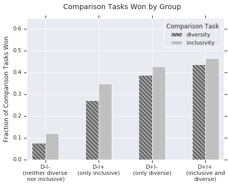
Figure 3. Fraction of comparison tasks “won” for each image group and task.

Data Quality

We screened for low-quality responses using three approaches: duplicate “confirmation questions”, the use of free-response fields on a multiple-choice question, and reCAPTCHA. First, each set of comparisons contained two “confirmation questions”, which were simply duplicates of earlier questions with images shuffled and the comparison presented in reverse order. Second, while the survey had only three available options (“Set A”, “Set B”, and “Same”), respondents were given a free-response answer box to type their answer. This allowed us to filter for automated responses, as we found that a small fraction of the responses were nonsensical (e.g. “No”, or “Very good”). Finally, respondents had to fill out a reCAPTCHA form before submitting. Answers with a reCAPTCHA score below $0.5$, those whose confirmation questions did not agree, and free-response answers that could not be resolved into a valid response were removed. After filtering, we had 491 valid responses, which contained comparisons between all image sets for each occupation.

Discussion

We have distinguished between notions of diversity and inclusion and detailed how they may be formalized, applied to the general problem of scoring instances or sets. This may be useful in subset selection problems that seek to reflect individuals with attributes that are disproportionately marginalized, such as when selecting images of people in a stock photo selection task. Our worked example demonstrates how social choice theory can be applied to compare diversity and inclusion scores across different sets.

- (1)
- Anari et al. (2016) Nima Anari, Shayan Oveis Gharan, and Alireza Rezaei. 2016. Monte Carlo Markov chain algorithms for sampling strongly Rayleigh distributions and determinantal point processes. In Conference on Learning Theory. 103–115.
- Asudeh et al. (2019) Abolfazl Asudeh, Zhongjun Jin, and HV Jagadish. 2019. Assessing and remedying coverage for a given dataset. In 2019 IEEE 35th International Conference on Data Engineering (ICDE). IEEE, 554–565.
- Barocas and Selbst (2016) Solon Barocas and Andrew D Selbst. 2016. Big data’s disparate impact. Calif. L. Rev. 104 (2016), 671.
- Baselga et al. (2007) Andrés Baselga, Alberto Jiménez-Valverde, and Gilles Niccolini. 2007. A multiple-site similarity measure independent of richness. Biology Letters 3, 6 (2007), 642–645.
- Bell and Hartmann (2007) Joyce M Bell and Douglas Hartmann. 2007. Diversity in everyday discourse: The cultural ambiguities and consequences of “happy talk”. American Sociological Review 72, 6 (2007), 895–914.
- Berrey (2015) Ellen Berrey. 2015. The Enigma of Diversity: The Language of Race and the Limits of Racial Justice. University of Chicago Press.
- Caragiannis et al. (2019) Ioannis Caragiannis, David Kurokawa, Hervé Moulin, Ariel D Procaccia, Nisarg Shah, and Junxing Wang. 2019. The unreasonable fairness of maximum Nash welfare. ACM Transactions on Economics and Computation (TEAC) 7, 3 (2019), 12.
- Celis et al. (2016) L Elisa Celis, Amit Deshpande, Tarun Kathuria, and Nisheeth K Vishnoi. 2016. How to be fair and diverse? arXiv preprint arXiv:1610.07183 (2016).
- Celis et al. (2017) L. Elisa Celis, Damian Straszak, and Nisheeth K. Vishnoi. 2017. Ranking with Fairness Constraints. CoRR abs/1704.06840 (2017). arXiv:1704.06840 http://arxiv.org/abs/1704.06840
- Cheryan et al. (2013) Sapna Cheryan, Victoria C Plaut, Caitlin Handron, and Lauren Hudson. 2013. The stereotypical computer scientist: Gendered media representations as a barrier to inclusion for women. Sex roles 69, 1-2 (2013), 58–71.
- Deshpande and Rademacher (2010) Amit Deshpande and Luis Rademacher. 2010. Efficient volume sampling for row/column subset selection. In 2010 IEEE 51st Annual Symposium on Foundations of Computer Science. IEEE, 329–338.
- Dobbin and Kalev (2016) Frank Dobbin and Alexandra Kalev. 2016. Why Diversity Programs Fail and What Works Better. Harvard Business Review 94, 7-8 (2016), 52–60.
- Drosou et al. (2017) Marina Drosou, HV Jagadish, Evaggelia Pitoura, and Julia Stoyanovich. 2017. Diversity in big data: A review. Big data 5, 2 (2017), 73–84.
- Dwork et al. (2012) Cynthia Dwork, Moritz Hardt, Toniann Pitassi, Omer Reingold, and Richard Zemel. 2012. Fairness through awareness. In Proceedings of the 3rd innovations in theoretical computer science conference. ACM, 214–226.
- Embrick (2011) David G Embrick. 2011. The diversity ideology in the business world: A new oppression for a new age. Critical sociology 37, 5 (2011), 541–556.
- Fitzpatrick (1988) Thomas B. Fitzpatrick. 1988. The Validity and Practicality of Sun-Reactive Skin Types I Through VI. JAMA Dermatology 124, 6 (06 1988), 869–871. https://doi.org/10.1001/archderm.1988.01670060015008
- Gong et al. (2014) Boqing Gong, Wei-Lun Chao, Kristen Grauman, and Fei Sha. 2014. Diverse sequential subset selection for supervised video summarization. In Advances in Neural Information Processing Systems. 2069–2077.
- Jost et al. (2009) Lou Jost et al. 2009. Mismeasuring biological diversity: response to Hoffmann and Hoffmann (2008). Ecological Economics 68, 4 (2009), 925–928.
- Kalev et al. (2006) Alexandra Kalev, Frank Dobbin, and Erin Kelly. 2006. Best practices or best guesses? Assessing the efficacy of corporate affirmative action and diversity policies. American sociological review 71, 4 (2006), 589–617.
- Kulesza et al. (2012) Alex Kulesza, Ben Taskar, et al. 2012. Determinantal point processes for machine learning. Foundations and Trends® in Machine Learning 5, 2–3 (2012), 123–286.
- Legendre et al. (2008) Pierre Legendre, Daniel Borcard, and Pedro R Peres-Neto. 2008. Analyzing or explaining beta diversity? Comment. Ecology 89, 11 (2008), 3238–3244.
- Lin and Bilmes (2012) Hui Lin and Jeff A Bilmes. 2012. Learning mixtures of submodular shells with application to document summarization. arXiv preprint arXiv:1210.4871 (2012).
- MacArthur (1965) Robert H MacArthur. 1965. Patterns of species diversity. Biological reviews 40, 4 (1965), 510–533.
- Mill (2016) John Stuart Mill. 2016. Utilitarianism. In Seven masterpieces of philosophy. Routledge, 337–383.
- Mor-Barak and Cherin (1998) Michal E Mor-Barak and David A Cherin. 1998. A tool to expand organizational understanding of workforce diversity: Exploring a measure of inclusion-exclusion. Administration in Social Work 22, 1 (1998), 47–64.
- Paradiso (2017) Anthony Paradiso. 2017. Diversity is Being Asked to the Party. Inclusion is Being Asked to Dance. #SHRMDIV. The Society for Human Resource Management (SHRM) Blog (2017). https://blog.shrm.org/blog/diversity-is-being-asked-to-the-party-inclusion-is-being-asked-to-dance-shr
- Pelled et al. (1999) Lisa H. Pelled, Gerald E Ledford, Jr, and Susan A. Mohrman. 1999. Demographic dissimilarity and workplace inclusion. Journal of Management studies 36, 7 (1999), 1013–1031.
- Rawls (1974) John Rawls. 1974. Some reasons for the maximin criterion. The American Economic Review 64, 2 (1974), 141–146.
- Roberson (2006) Quinetta M Roberson. 2006. Disentangling the meanings of diversity and inclusion in organizations. Group & Organization Management 31, 2 (2006), 212–236.
- Samadi et al. (2018) Samira Samadi, Uthaipon Tantipongpipat, Jamie H Morgenstern, Mohit Singh, and Santosh Vempala. 2018. The price of fair PCA: One extra dimension. In Advances in Neural Information Processing Systems. 10976–10987.
- Shore et al. (2011) Lynn M Shore, Amy E Randel, Beth G Chung, Michelle A Dean, Karen Holcombe Ehrhart, and Gangaram Singh. 2011. Inclusion and diversity in work groups: A review and model for future research. Journal of management 37, 4 (2011), 1262–1289.
- Singh and Joachims (2017) Ashudeep Singh and Thorsten Joachims. 2017. Equality of opportunity in rankings. In Workshop on Prioritizing Online Content (WPOC) at NIPS.
- Snell (2017) Tonie Snell. 2017. Tokenism: The Result of Diversity Without Inclusion. Medium (2017). https://medium.com/@TonieSnell/tokenism-the-result-of-diversity-without-inclusion-460061db1eb6
- Tuomisto (2011) Hanna Tuomisto. 2011. Commentary: do we have a consistent terminology for species diversity? Yes, if we choose to use it. Oecologia 167, 4 (2011), 903–911.
- Whittaker (1960) Robert Harding Whittaker. 1960. Vegetation of the Siskiyou mountains, Oregon and California. Ecological monographs 30, 3 (1960), 279–338.
- Yang and Stoyanovich (2017) Ke Yang and Julia Stoyanovich. 2017. Measuring fairness in ranked outputs. In Proceedings of the 29th International Conference on Scientific and Statistical Database Management. ACM, 22.
- Zhou et al. (2010) Tao Zhou, Zoltán Kuscsik, Jian-Guo Liu, Matúš Medo, Joseph Rushton Wakeling, and Yi-Cheng Zhang. 2010. Solving the apparent diversity-accuracy dilemma of recommender systems. Proceedings of the National Academy of Sciences 107, 10 (2010), 4511–4515.