A comparison of Bayesian accelerated failure time models with spatially varying coefficients

Abstract

The accelerated failure time (AFT) model is a commonly used tool in analyzing survival data. In public health studies, data is often collected from medical service providers in different locations. Survival rates from different locations often present geographically varying patterns. In this paper, we focus on the accelerated failure time model with spatially varying coefficients. We compare a three different types of the priors for spatially varying coefficients. A model selection criterion, logarithm of the pseudo-marginal likelihood (LPML), is developed to assess the fit of AFT model with different priors. Extensive simulation studies are carried out to examine the empirical performance of the proposed methods. Finally, we apply our model to SEER data on prostate cancer in Louisiana and demonstrate the existence of spatially varying effects on survival rates from prostate cancer.

Keywords: Geographical Pattern; Prostate Cancer; MCMC; Survival Model

1 Introduction

Patient data in public health studies is often collected on certain administrative divisions such as counties or provinces. Oftentimes, the patient group in different regions have similar characteristics yet exhibit different patterns of survival outcomes, which leads us to investigate in the geographical variation of covariate effects.

There is much recent work analyzing geographical patterns of survival data. For example, Henderson et al. (2002) used the proportional hazards model to model spatial variation in survival of leukemia patients in northwest England; Banerjee and Dey (2005) applied a spatial frailty model to infant mortality in Minnesota by using geostatistical or Gaussian Markov random field priors for the spatial component; Zhou et al. (2008) applied the conditional autoregressive (CAR) model in a parametric survival model to construct a joint spatial survival model for prostate cancer data, and Zhang and Lawson (2011) modeled the spatial random effects in an accelerated failure rate (AFT) model using the CAR prior. In all these works, spatial variation is modeled as spatial random effect, while the variation in the covariate effects for risk factors are not accounted for. From the spatially varying coefficients perspective, Gelfand et al. (2003) proposed a model that allows the coefficients in a regression model to vary at the local or subregional level by viewing them as realizations of a Gaussian process with a certain covariance structure that is decided by the relationship between spatial locations. Reich et al. (2010); Boehm Vock et al. (2015) applied spatially varying coefficients in a generalized linear model to investigate the health effects of fine particulate matter components. An application of the spatially varying coefficients methodology to the Cox model was proposed in Xue et al. (2019) from the frequentist perspective.

In this work, we propose a Bayesian AFT model with spatially varying coefficients. Specifically, the variation in coefficient vectors is modeled using three different priors: Gaussian, CAR, and the Dirichlet process (DP), corresponding to different possible true underlying variation patterns. A model selection criterion, logarithm of the pseudo-marginal likelihood (LPML), is employed to assess the fitness of three different priors. Our simulation studies showed promising empirical performance of the proposed methods in both non-spatially varying and spatially varying cases. Furthermore, our proposed criterion also select the best fitness model. In addition, our proposed Bayesian approach reveals interesting features of the prostate cancer data for Louisiana.

The rest of this paper is organized as follows. In Section 2 we propose the Bayesian AFT model with spatially varying coefficients for both uni-covariate and multi-covariate cases. Three prior distributions used to account for the spatial variation are introduced. In Section 3, we present the computation for the proposed model using the powerful R package nimble (de Valpine et al., 2017), and propose the corresponding model selection technique using the LPML. Simulation studies are conducted in Section 4, and we illustrate its practical use in Section 5 using the prostate cancer data for Louisiana from the SEER program. We conclude the paper with a brief discussion in Section 6.

2 The Bayesian AFT

2.1 AFT with Spatially Varying Coefficients

Let $T_{\ell}(s_{i})$ denote the survival time for patient $\ell$ at location $s_{i}$, and $X_{\ell}(s_{i})$ denote a covariate corresponding to $T_{\ell}(s_{i})$, where $i=1,2,...,n$, and $\ell=1,2,...,n_{i}$, with $n_{i}$ denoting the number of the patients at $s_{i}$. We propose the following spatial AFT model:

$$\log(T_{\ell}(s_{i}))=\tilde{\beta}_{0}(s_{i})+X_{\ell}(s_{i})\tilde{\beta}_{1}(s_{i})+\sigma(s_{i})\epsilon_{\ell}(s_{i}),$$ (1)

where $\tilde{\beta}_{1}(s_{i})=\beta_{1}+\beta_{1}(s_{i})$ is the slope at location $s_{i}$, $\tilde{\beta}_{0}(s_{i})=\beta_{0}+\beta_{0}(s_{i})$ is the intercept at location $s_{i}$, $\sigma(s_{i})$ is the scale parameter at location $s_{i}$, and the $\epsilon_{l}(s_{i})$’s are i.i.d. random errors. The term $\beta_{1}(s_{i})$ can be regarded as a random spatial adjustment at location $s_{i}$ to the overall slope $\beta_{1}$.

Let $f(t_{\ell}(s_{i}))$ be the density function of $T_{\ell}(s_{i})$ and $f_{0}(\cdot)$ denote the density function of $\epsilon_{\ell}(s_{i})$. Further, denote the survival function of $T_{\ell}(s_{i})$ as $S(t_{\ell}(s_{i}))$, and of $\epsilon_{\ell}(s_{i})$ as $S_{0}(\cdot)$. We consider right-censored survival observations $(t_{\ell}(s_{i}),\delta_{\ell}(s_{i}))$, where $\delta_{\ell}(s_{i})=1(t_{\ell}(s_{i})\leq C_{\ell}(s_{i}))$ with 1() being the indicator function, $C_{\ell}(s_{i})$ being the censoring time. Then the likelihood function can be written as:

$$L=\prod_{i=1}^{n}\prod_{\ell=1}^{n_{i}}f(t_{l}(s_{i}))^{\delta_{\ell}(s_{i})}S(t_{\ell}(s_{i}))^{1-\delta_{\ell}(s_{i})},$$ (2)

where

$$\begin{split}f(t_{\ell}(s_{i}))&=\frac{1}{\sigma(s_{i})t_{\ell}(s_{i})}f_{0}(\log(t_{i}(s_{i}))-(\tilde{\beta}_{0}(s_{i})+X(s_{i})\tilde{\beta}_{1}(s_{i}))/\sigma(s_{i})),\\ S(t_{\ell}(s_{i}))&=S_{0}(\log(t_{\ell}(s_{i}))-(\tilde{\beta}_{0}(s_{i})+X(s_{i})\tilde{\beta}_{1}(s_{i}))/\sigma(s_{i}))\,.\end{split}$$

In a parametric model, $S_{0}(.)$ can be assumed to be the standard normal distribution, the standard extreme value distribution, or the logistic distribution, etc. They lead to different distributions (e.g., exponential distribution, Weibull distribution, log-logistic distribution and log- normal distribution) for the survival times $T_{\ell}(s_{i})$ to complete the model specification.

Now, instead of considering a single covariate, we consider a $p$-dimensional covariate vector for each observation. Let $\bm{X}_{\ell}(s_{i})$ be the covariate vector for patient $\ell$ at location $s_{i}$, where $\bm{X}_{\ell}(s_{i})$ includes an initial $1$ (for the intercept). Equation (1) can be written into the following form:

$$\log(T_{\ell}(s_{i}))=\bm{X}_{\ell}(s_{i})\bm{\tilde{\beta}}(s_{i})+\sigma(s_{i})\epsilon_{\ell}(s_{i}),~{}~{}\ell=1,\ldots,n_{i},~{}i=1,\ldots,n.$$ (3)

2.2 Gaussian Process Prior

The most straightforward prior for spatially varying coefficients is the Gaussian process prior (Gelfand et al., 2003). The Gaussian process prior assumes that:

$${\tilde{\bm{\beta}}}\mid\bm{\mu}_{\bm{\beta}},\bm{T}\sim\mbox{MVN}(1_{n\times 1}\otimes\bm{\mu}_{\bm{\beta}},\bm{H}(\phi)\otimes\bm{T})$$ (4)

where ${\tilde{\bm{\beta}}}=(\tilde{\bm{\beta}}(\bm{s}_{1})^{\top},\ldots,\tilde{\bm{\beta}}(\bm{s}_{n})^{\top})^{\top}$, $\bm{\mu}_{\bm{\beta}}$ is a $p\times 1$ vector, $\bm{H}(\phi)$ is a $n\times n$ matrix of spatial correlations between the $n$ observed locations, $\bm{T}$ is a $p\times p$ covariance matrix associated with an observation vector at any spatial location, and $\otimes$ denotes the Kronecker product. The $(i,j)$th entry of $\bm{H}(\phi)$ is $\exp(-\phi|\bm{s}_{i}-\bm{s}_{j}|)$, where $|\bm{s}_{i}-\bm{s}_{j}|$ is the distance between $\bm{s}_{i}$ and $\bm{s}_{j}$, and $\phi$ is the range parameter for spatial correlation. For the Gaussian process prior, the regression coefficients of closer locations have strong correlation.

2.3 Conditional Autoregressive Prior

From Banerjee et al. (2014), if the spatial domain $D$ is fixed and is partitioned into a finite number of areal units $(A_{1},\cdots,A_{n})$ with boundaries, data collected from such areal units, such as cancer patients in counties of a state, is known as areal data. For areal data, the spatial association depends on neighborhood structures. Generally, the neighborhood structure for $n$ areal units comes from an $n\times n$ adjacency matrix $W$, where $w_{ij}=1$ if areal units $A_{i}$ and $A_{j}$ share a common boundary, and 0 otherwise. The conditional autoregressive model (CAR; Besag, 1974) is one of the most popular tools to model spatial correlations. It also has an advantage for being computationally efficient for Gibbs sampling. For Gaussian spatial random effects $\bm{\phi}=(\phi(A_{1}),\cdots,\phi(A_{n}))$, the CAR model is defined as:

$$\phi(A_{i})\mid\phi(A_{-i})\sim N(\rho\sum_{j\neq i}w_{ij}\phi(A_{j}),\tau^{2}),$$ (5)

where $\phi(A_{-i})=\{\phi(A_{j}),j\neq i\}$, $\tau^{2}$ is the conditional variance, and $\rho\in\mathcal{R}$. Under the Brook’s Lemma (Brook, 1964), we can obtain the joint distribution of $\bm{\phi}$ as:

$$p(\phi(A_{1}),\cdots,\phi(A_{n}))\propto\exp\left\{-\frac{1}{2}\bm{\phi}^{\prime}D^{-1}(I-\rho W)\bm{\phi}\right\},$$ (6)

where $D$ is diagonal matrix with $D_{ii}=\tau^{2}$. Equation (6) suggests that $\bm{\phi}$ follows a multivariate normal distribution with mean $\bm{0}$ and variance covariance matrix $\tau^{2}(I-\rho W)^{-1}$. This requires that $W$ be symmetric and $\tau^{2}(I-\rho W)^{-1}$ be positive definite. Let $\lambda_{1}\leq\cdots\lambda_{n}$ be the eigenvalues of $W$. The eigenvalues sum to 0 since $\text{trace}(W)=0$ which tells us that $\lambda_{1}<0<\lambda_{n}$. The matrix $I-\rho W$ is positive definite if and only if $\rho\in(1/\lambda_{1},1/\lambda_{n})$. Based on the joint distribution of CAR model, we have Conditional Autoregressive type prior for spatially varying coeffcients:

$$\begin{split}\tilde{\bm{\beta}}_{j}\sim\mbox{MVN}(\bm{0},\tau^{2}_{j}(I-\rho W)^{-1}),\\ \tau^{2}_{j}\sim\mbox{IG}(a,b),\\ \rho\sim\text{Unif}(1/\lambda_{1},1/\lambda_{n}),\end{split}$$ (7)

where $\tilde{\bm{\beta}}_{j}=(\tilde{\beta}_{j}(\bm{s}_{1}),\ldots,\tilde{\beta}_{j}(\bm{s}_{n}))^{\prime}$, $j=1,\ldots,p$.

2.4 Dirichlet Process Mixture Prior

Within the Bayesian framework, Dirichlet process mixture model (DPMM) can link response variable to covariates through cluster membership (Molitor et al., 2010). Formally, a probability measure $G$ following a Dirichlet process (DP; Ferguson, 1973) with a concentration parameter $\alpha$ and a base distribution $G_{0}$ is denoted by $G\sim\text{DP}(\alpha,G_{0})$ if

$$(G(A_{1}),\cdots,G(A_{r}))\sim\text{Dirichlet}(\alpha G_{0}(A_{1}),\cdots,\alpha G_{0}(A_{r})),$$ (8)

where $(A_{1},\cdots,A_{r})$ are finite measurable partitions of the space $\Omega$.

Several different formulations can be used for determining the DP. In this work, we use the stick-breaking construction proposed by Sethuraman (1991) for DP realization, which is given as

$$\begin{split}\theta_{c}\sim G_{0},\hskip 2.84544ptG=\sum_{c=1}^{\infty}\pi_{c}\delta_{\theta_{c}}(\cdot),\\ \pi_{1}=V_{1},\hskip 2.84544pt\pi_{c}=V_{c}\prod_{\ell<c}(1-V_{\ell}),\\ V_{c}\sim\text{Beta}(1,\alpha),\end{split}$$

where $\theta_{c}$ is the $c$th matrix consisting of the possible values for the parameters of $G_{0}$, $\delta_{\theta_{c}}(\cdot)$ denotes a discrete probability measure concentrated at $\theta_{c}$, and $\pi_{c}$ is the random probability weight between 0 and 1.

Based on the DPMM, we can model the the spatially varying coefficients as following the Dirichlet process gaussian mixture prior with $G_{0}$ being the multivariate normal distribution :

$$\begin{split}\bm{\beta}_{z_{i}}\stackrel{{\scriptstyle\text{ind}}}{{\sim}}\mbox{MVN}(\bm{\mu},\bm{\Sigma}),\\ P(z_{i}=c\mid\bm{\pi})=\pi_{c},\\ \pi_{1}=V_{1},\hskip 2.84544pt\pi_{c}=V_{c}\prod_{\ell<c}(1-V_{\ell}),\hskip 2.84544ptV_{c}\sim\text{Beta}(1,\alpha),\\ \tilde{\bm{\beta}}(\bm{s}_{i})=\sum_{i=1}^{\infty}\pi_{i}\bm{\beta}_{z_{i}},\end{split}$$ (9)

where $\bm{\mu}$ and $\bm{\Sigma}$ are hyper parameters for the multivariate normal distribution.

3 Bayesian Inference

In this section, we present the code used for computation using nimble (de Valpine et al., 2017). Also, as we discussed in the introduction that Gaussian, CAR, and DP can all be used as the prior for modeling the variation in the coefficient vector and a choice needs to be made among these three, the model selection criterion LPML is discussed.

3.1 Bayesian Computation

A nimble model consists of four major parts: model code, model constants, data, and the initial values for MCMC. The model code is syntactically similar to the BUGS language. As an illustration, we denote the number of locations as $m$, number of observations per county as $n$, and dimension of the covariate vector as $p=3$. Take the model with CAR prior as an example. First, the model is defined using the nimbleCode() function:

aft_car ¡- nimbleCode({
    for (i in 1:m) {
        for (j in 1:n) {
            logtime[i, j] ~ dnorm(mu[i, j], sigma[i])
            censor[i, j] ~ dinterval(logtime[i, j], censortime[i, j])
            mu[i, j] ¡- inprod(beta[z[i], 1:p], X[1:p, i, j])

        }
        sigma[i] ~ dinvgamma(1, 1)
    }
    correlation[1:m, 1:m] ¡- diag(1, m) - b * W
    b ~ dunif(low, high)
    for (i in 1:p) {
        prec[i, 1:m, 1:m] ¡- sigmabeta[i] * correlation[1:m, 1:m]
        beta[1:m, i] ~ dmnorm(mu_beta[1:m], prec = prec[i, 1:m, 1:m])
        sigmabeta[i] ~ dgamma(1, 1)
    }
})

The 4th row of code defines that the logarithm of survival time for the $j$th observation from the $i$th county follows normal distribution with mean mu[i, j] and standard deviation sigma[i], wich corresponds to Equation (3). Next, due to the existence of censoring, the censoring indicator censor[i, j] equals 1 if logtime[i, j] is right censored, and 0 otherwise. The normal mean mu[i,j] is connected to the covariate vector of the corresponding observation via inprod(beta[z[i], 1:p], X[1:p, i, j]). For county $i$, its corresponding scale parameter is set to have an inverse gamma distribution with shape 1 and scale 1. The correlation matrix is set to be $I-bW$ as in (6) with $\rho$ replaced by b. The two endpoints low and high correspond to $1/\lambda_{1}$ and $1/\lambda_{n}$ in (7).

In the second part, we declare the data list for the model, which include the logarithm of observed survival times, indicator for censoring, the independent variables $X$, the adjacency matrix $W$, and the censor times.

data ¡- list(
    logtime = logtime,
    censor = censor,
    X = X,
    adjacency = W,
    censortime = censortime
)

Next we set the list of constant quantities in the model code. The quantities low and high are obtained based on the adjacency structure of Louisiana counties.

constants ¡- list(
    n = 100,
    m = 64,
    mu_beta = rep(0, m),
    p = 3,
    low = -0.358,
    high = 0.175
)

Finally, the initial values for parameters are assigned.

inits ¡- list(
    beta = matrix(0, m, p),
    b = 0,
    sigma = rep(1, m),
    sigmabeta = rep(1, p)
)

With all four parts properly defined, nimble provides an one-line implementation to invoke the MCMC engine, which includes setting the chain length, burn-in, thinning, etc.:

mcmc.out ¡- nimbleMCMC(
        model = aftModel,
        niter = 20000,
        nchains = 1,
        nburnin = 5000,
        thin = 1,
        monitors = c("b", "sigma", "beta", "sigmabeta"),
        summary = TRUE
    )

The configuration above indicates that the MCMC results of parameters b, sigma, beta, and sigmabeta. One chain is ran for 20000 iterations with the first 5000 as burnin and without thinning. Therefore, finally we obtain 15000 samples for each parameter.

3.2 Bayesian Model Selection

A commonly used model comparison criterion, the Logarithm of the Pseudo-Marginal Likelihood (LPML; Ibrahim et al., 2013), is applied to model selection. The LPML can be obtained through the Conditional Predictive Ordinate (CPO) values. Let $Y_{(-i)}=\{Y_{j}:j=1,\cdots,i-1,i+1,n\}$ denote the observations with the $i$th subject response deleted. The CPO for the $i$th subject is defined as:

$$\text{CPO}_{i}=\int f(Y_{i}\mid\tilde{\bm{\beta}}(s_{i})\pi(w(s),\tilde{\bm{\beta}(s)},\sigma_{y}^{2}\mid Y_{(-i)})\differential(w(s),\bm{\beta}(s),\sigma_{y}^{2}),$$ (10)

where

$$\pi(w(s),\bm{\beta}(s),\sigma_{y}^{2}\mid Y_{(-i)})=\frac{\prod_{j\neq i}f(y(s_{j})\mid\bm{\beta}(s),w(s),\sigma_{y}^{2})\pi(w(s),\bm{\beta}(s),\sigma_{y}^{2}\mid Y_{(-i)})}{c(Y_{(-i)})},$$

and $c(Y_{(-i)})$ is the normalizing constant. Within the Bayesian framework, a Monte Carlo estimate of the CPO can be obtained as:

$$\widehat{\text{CPO}}_{i}^{-1}=\frac{1}{T}\sum_{t=1}^{T}\frac{1}{f(Y_{i}\mid\tilde{\bm{\beta}}_{t}(\bm{s}_{i}),\sigma(\bm{s}_{i})},$$ (11)

where $T$ is the total number of Monte Carlo iterations. An estimate of the LPML can subsequently be calculated as:

$$\widehat{\text{LPML}}=\sum_{i=1}^{N}\text{log}(\widehat{\text{CPO}}_{i}).$$ (12)

Intuitively, a larger LPML indicates better fit to the data, and the corresponding model is more preferred.

4 Simulation

In this section, we present simulation studies for scenarios where there is no spatial variation in the covariate effects, and where there is indeed spatial variation in the covariate effects. Information of the 64 Louisiana counties, including their centroids and their adjacency structure, is used. After obtaining the final parameter estimates and their 95% highest posterior density (HPD) intervals, we evaluate them using the following four performance measures:

$$\begin{split}\text{mean absolute bias (MAB)}&=\frac{1}{64}\sum_{\ell=1}^{64}\frac{1}{100}\sum_{r=1}^{100}\left|\hat{\beta}_{\ell,m,r}-\beta_{\ell,m}\right|,\\ \text{mean of mean squared error (MMSE)}&=\frac{1}{64}\sum_{\ell=1}^{64}\frac{1}{100}\sum_{r=1}^{100}\left(\hat{\beta}_{\ell,m,r}-\beta_{\ell,m}\right)^{2},\\ \text{mean standard deviation (MSD)}&=\frac{1}{64}\sum_{\ell=1}^{64}\sqrt{\frac{1}{99}\sum_{r=1}^{100}\left(\hat{\beta}_{\ell,m,r}-\bar{\hat{\beta}}_{\ell,m}\right)^{2}},\\ \text{mean coverage rate (MCR)}&=\frac{1}{64}\sum_{\ell=1}^{64}\frac{1}{100}\sum_{r=1}^{100}\text{1}\left(\beta_{\ell,m}\in 95\%\text{ HPD interval for replicate $r$}\right),\end{split}$$

where $\beta_{\ell,m}$ denotes the true value of the parameter for the $m$th covariate in the $\ell$th county, $\bar{\hat{\beta}}_{\ell,m}$ is the average of point estimates in the 100 replicates of simulation, $\beta_{\ell,m}$ denotes the true underlying parameter, and $1()$ denotes the indicator function. In addition, the performance of DP prior in clustering the counties is assessed with the Rand Index (RI; Rand, 1971), whose value being close to 1 indicates good clustering result. The code used is available at GitHub (https://github.com/nealguanyu/Bayesian_AFT_SVC).

4.1 Simulation Without Spatially Varying Coefficients

First we consider the scenario where there is no spatial variation in the coefficients. Survival data are generated with $\beta=(0.6,0.35,-0.5)^{\top}$. Censoring times are generated independently from $\mbox{Exp}(1)$. Next, the three models are fitted to the datasets. For each of the 64 counties considered, three covariates are generated for 100 observations identically and independently from $N(0,1)$. Chain lengths are set to 50,000 with the first 20,000 as burn-in. With the thinning interval set to 10, a total of 3,000 posterior samples are obtained for each replicate. The performance of Bayesian spatial AFT with the three aforementioned priors is reported in Table 1. The average point estimates over the 100 replicates and 64 counties are reported as well. For DP prior, the maximum number of clusters is initially set to 20.

It turns out that under the no spatial variation scenario, models based on all three priors give similar and rather accurate estimation results. The Gaussian and CAR priors, as they allow each location to have their own set of parameter, give relatively more volatile parameter estimates than the DP prior, as in all 100 replicates the 64 counties are identified to be in the same cluster, and the parameter estimates are essentially coming from a model where all observations are used. The MAB, MMSE, MSD of parameter estimates given by the model with DP prior are much smaller than those given by the other two models. The MCR, as a consequence, is lower than MCR for Gaussian and CAR prior, but is still close to the 0.95 nominal value.

Table 1: Average point estimates as well as the four performance measures for estimation under the null scenario without spatially varying coefficients for the three priors.

Prior	Parameter	Point Estimate	MAB	MMSE	MSD	MCR
Gaussian	$\beta_{1}$	0.608	0.039	0.002	0.049	0.992
	$\beta_{2}$	0.374	0.044	0.003	0.050	0.978
	$\beta_{3}$	-0.519	0.043	0.003	0.050	0.986
CAR	$\beta_{1}$	0.565	0.085	0.011	0.099	0.944
	$\beta_{2}$	0.326	0.079	0.010	0.094	0.951
	$\beta_{3}$	-0.473	0.082	0.011	0.097	0.944
DP	$\beta_{1}$	0.598	0.011	0.0002	0.014	0.930
	$\beta_{2}$	0.357	0.011	0.0002	0.013	0.930
	$\beta_{3}$	-0.509	0.013	0.0002	0.013	0.920

4.2 Simulation with Spatially Varying Coefficients

We consider a smooth variation of coefficients over the counties of Louisiana. The latitude and longitude of county centroids are obtained, and normalized to have mean 0 and standard deviation 1. For county $\ell$, the coefficient vector

$$\beta_{\ell}^{\top}=(0.6,0.35,-0.5)+0.1\times(\mbox{longitude}_{\ell}+\mbox{latitude}_{\ell}),~{}~{}\ell=1,\ldots,64,$$ (13)

where $\mbox{latitude}_{\ell}$ and $\mbox{longitude}_{\ell}$ denote the normalized coordinates, respectively. Other data generation settings are consistent with Section 4.1. Each of the three priors are fitted on the same 100 replicates of simulated data. Results are reported in Table 2. In another case, instead of having the variation pattern depend on longitude and latitude of county centroids, we considered the case where there is a small random term at each county, i.e,

$$\beta_{\ell}^{\top}=(0.6,0.35,-0.5)+\Delta\beta^{\top},$$ (14)

where $\Delta\beta\sim\mbox{MVN}(\bm{0},0.1\bm{I}_{3})$. Corresponding results are presented in Table 3.

Table 2: Performance measures for estimation under the alternative scenario (13) for the three priors.

Prior	Parameter	MAB	MMSE	MSD	MCR
Gaussian	$\beta_{1}$	0.042	0.003	0.051	0.988
	$\beta_{2}$	0.046	0.003	0.051	0.974
	$\beta_{3}$	0.045	0.003	0.052	0.983
CAR	$\beta_{1}$	0.086	0.012	0.101	0.938
	$\beta_{2}$	0.080	0.010	0.095	0.944
	$\beta_{3}$	0.083	0.011	0.099	0.942
DP	$\beta_{1}$	0.074	0.010	0.074	0.397
	$\beta_{2}$	0.073	0.009	0.068	0.403
	$\beta_{3}$	0.073	0.009	0.068	0.403

Table 3: Performance measures for estimation under the alternative scenario (14) for the three priors.

Prior	Parameter	MAB	MMSE	MSD	MCR
Gaussian	$\beta_{1}$	0.065	0.007	0.060	0.932
	$\beta_{2}$	0.065	0.007	0.058	0.916
	$\beta_{3}$	0.066	0.007	0.060	0.919
CAR	$\beta_{1}$	0.087	0.012	0.101	0.941
	$\beta_{2}$	0.081	0.010	0.095	0.952
	$\beta_{3}$	0.084	0.011	0.099	0.943
DP	$\beta_{1}$	0.086	0.011	0.037	0.214
	$\beta_{2}$	0.069	0.008	0.022	0.323
	$\beta_{3}$	0.073	0.008	0.025	0.267

From Tables 2 and 3, it is not surprising that the Gaussian and CAR priors still give rather credible estimation results. The DP prior, however, despite having MAB, MMSE and MSD roughly on the same scale, has much lower MCR, which is due to the fact that in order to detect clustered covariate effects, we are limiting the maximum number of clusters to 20. With such specification yet a continuously varying parameter surface (13) or a randomly varying parameter surface (14), failure for the DP parameter estimates to cover some of the true values is inevitable.

Similar to in Ma et al. (2019), we also consider a setting where counties in a region share the same covariate effects. The three-region partition of Louisiana counties as illustrated in Figure 1 is considered. Under this setting, the RI for DP prior over the 100 replicates averages to more than 0.972, indicating highly accurate clustering performance. Compared to the Gaussian and CAR priors, the DP prior again yields parameter estimates that are more stable, having much smaller MAB, MMSE, and MSD. As a consequence of under-clustering in some replicates, i.e., less than three clusters are identified, the MCR of DP prior is lower than the other two, but still close to or higher than 0.85.

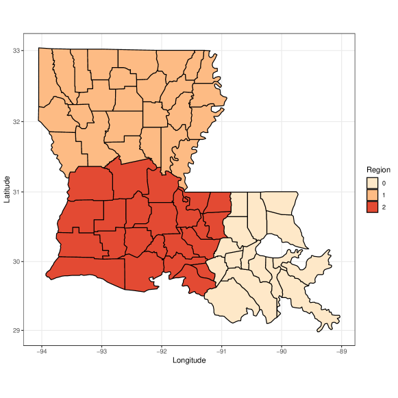
Figure 1: Illustration for the partition of Louisiana counties into three regions.

Table 4: Performance measures for estimation under the alternative regional scenario for the three priors.

Prior	Parameter	MAB	MMSE	MSD	MCR
Gaussian	$\beta_{1}$	0.150	0.035	0.171	0.961
	$\beta_{2}$	0.187	0.051	0.152	0.893
	$\beta_{3}$	0.218	0.069	0.169	0.870
CAR	$\beta_{1}$	0.187	0.055	0.222	0.954
	$\beta_{2}$	0.193	0.059	0.205	0.941
	$\beta_{3}$	0.216	0.073	0.202	0.906
DP	$\beta_{1}$	0.046	0.013	0.108	0.898
	$\beta_{2}$	0.042	0.011	0.103	0.898
	$\beta_{3}$	0.044	0.009	0.089	0.845

5 Survival Analysis of SEER Prostate Cancer Patients

We use the dataset on prostate cancer patients from the SEER program as an illustration for applicability of the proposed methods. There are 31,271 patients diagnosed with prostate cancer between 1973 to 2013, 2,057 of which experienced events due to prostate cancer within the follow-up period, resulting in a state-level censoring rate of 93.4%. Three risk factors are considered in our analysis: age at diagnosis (Age, centered and scaled), marital status indicator (Married), and indicator for being non-White (Race). Survival times are reported in integer months. For those whose observed time is 0, a minor 0.0001 adjustment term is added to the survival time to avoid negative infinity log times. The demographic characteristics for this dataset is presented in Table 5. In Figure 2, number of observations and per-county Kaplan–Meier (KM) survival probability estimates at 50 months after diagnosis are plotted on the map of Louisiana. Tensas county has the smallest number of observations (37), and East Baton Rouge has the largest number of observations (3614). At 50 months after diagnosis, the KM survival probability is highest for East Carroll (0.972), and lowest for Allen (0.658).

Table 5: Demographics for the studied dataset. For continuous variables, the mean and standard deviation (SD) are reported. For binary variables, the frequency and percentage of each class are reported.

	Mean(SD) / Frequency (Percentage)
Age	64.78 (10.89)
Survival Time	63.77 (43.09)
Event	40.02 (33.90)
Censor	65.44 (43.17)
Marital Status
Currently Married	26 558 ($84.93\%$)
Other	4 713 ($15.07\%$)
Race
White	21 674 ($69.31\%$)
Other	9 597 ($30.69\%$)
Cause-specific Death Indicator
Event	2 057 ($6.58\%$)
Censor	29 214 ($93.42\%$)

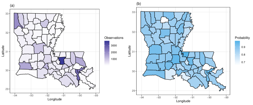
Figure 2: (a) Number of observations in counties of Louisiana; (b) Kaplan–Meier estimate of survival probability at 50 months after diagnosis in each county.

Estimation using each of the three priors discussed before is done on the dataset. To determine which prior yields estimation that best suit the data, the LPML values are calculated and reported in Table 6. As a larger LPML value indicates a better fit, we choose to base our final conclusion on the CAR prior model’s results. In addition, to verify that covariates are indeed varying, a vanilla model with no spatially varying effects is fitted, and it turns out to have an LPML value of -595 240.9, indicating the existence of such effects. In addition, it can be noticed that the DP prior based model has the smallest LPML value, as it only identifies two clusters, and does not make the model flexible enough.

Final estimation results are visualized on the county-level map of Louisiana in Figure 3. The overall pattern aligns with our intuition. The parameter estimates for Age are negative in all counties, indicating that older patients on average are more likely to experience an event than younger patients. The parameter estimates for Race is also negative in all counties, which suggests that there exist racial disparities in the outcome of healthcare for prostate cancer in Louisiana. Finally, compared to others, married patients are, on average, surviving for longer times. In addition, the spatial variation in all three covariate effects is rather clear.

Table 6: LPML values for different priors in modeling Louisiana data.

	Gaussian Process	CAR	DP
LPML	-406 588.20	-367 700.24	-416 597.30

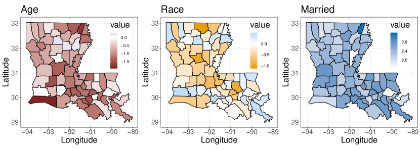
Figure 3: Visualization of final covariate effect estimates for Louisiana counties.

6 Discussion

We proposed the usage of three different prior distributions in Bayesian estimation of the spatially varying coefficients for the AFT model. The three priors all have accurate performance under the null scenario where there is no spatial variation, and are able to identify the varying patterns and produce highly accurate parameter estimates under each of the three alternative scenarios. In addition, when the spatial variation pattern is not smooth but clustered, the DP prior is able to produce credible inference of cluster belongings. The practical merit of the proposed method is illustrated using a SEER prostate cancer data of patients in Louisiana.

A few issues are worth further investigating. In this work and many other previous works in the spatially varying coefficients model context, oftentimes all $p$ covariates are assumed to vary, which can lead to unnecessarily large models if there are some coefficients are not varying. Identifying such coefficients is an interesting topic. Extension of the proposed methods to the proportional hazards model is also dedicated to future research.

References

- Banerjee et al. (2014) Banerjee, S., B. P. Carlin, and A. E. Gelfand (2014). Hierarchical Modeling and Analysis for Spatial Data. Crc Press.
- Banerjee and Dey (2005) Banerjee, S. and D. K. Dey (2005). Semiparametric proportional odds models for spatially correlated survival data. Lifetime Data Analysis 11(2), 175–191.
- Besag (1974) Besag, J. (1974). Spatial interaction and the statistical analysis of lattice systems. Journal of the Royal Statistical Society: Series B (Methodological) 36(2), 192–225.
- Boehm Vock et al. (2015) Boehm Vock, L. F., B. J. Reich, M. Fuentes, and F. Dominici (2015). Spatial variable selection methods for investigating acute health effects of fine particulate matter components. Biometrics 71(1), 167–177.
- Brook (1964) Brook, D. (1964). On the distinction between the conditional probability and the joint probability approaches in the specification of nearest-neighbour systems. Biometrika 51(3/4), 481–483.
- de Valpine et al. (2017) de Valpine, P., D. Turek, C. J. Paciorek, C. Anderson-Bergman, D. T. Lang, and R. Bodik (2017). Programming with models: writing statistical algorithms for general model structures with NIMBLE. Journal of Computational and Graphical Statistics 26(2), 403–413.
- Ferguson (1973) Ferguson, T. S. (1973). A Bayesian analysis of some nonparametric problems. Annals of Statistics 1(2), 209–230.
- Gelfand et al. (2003) Gelfand, A. E., H.-J. Kim, C. Sirmans, and S. Banerjee (2003). Spatial modeling with spatially varying coefficient processes. Journal of the American Statistical Association 98(462), 387–396.
- Henderson et al. (2002) Henderson, R., S. Shimakura, and D. Gorst (2002). Modeling spatial variation in leukemia survival data. Journal of the American Statistical Association 97(460), 965–972.
- Ibrahim et al. (2013) Ibrahim, J. G., M.-H. Chen, and D. Sinha (2013). Bayesian Survival Analysis. Springer Science & Business Media.
- Ma et al. (2019) Ma, Z., Y. Xue, , and G. Hu (2019). Geographically weighted regression analysis for spatial economics data: A Bayesian recourse. Technical Report 19-10, University of Connecticut, Department of Statistics.
- Molitor et al. (2010) Molitor, J., M. Papathomas, M. Jerrett, and S. Richardson (2010). Bayesian profile regression with an application to the National survey of children’s health. Biostatistics 11(3), 484–498.
- Rand (1971) Rand, W. M. (1971). Objective criteria for the evaluation of clustering methods. Journal of the American Statistical Association 66(336), 846–850.
- Reich et al. (2010) Reich, B. J., M. Fuentes, A. H. Herring, and K. R. Evenson (2010). Bayesian variable selection for multivariate spatially varying coefficient regression. Biometrics 66(3), 772–782.
- Sethuraman (1991) Sethuraman, J. (1991). A constructive definition of Dirichlet priors. Statistics Sinica 4(2), 639–650.
- Xue et al. (2019) Xue, Y., E. D. Schifano, and G. Hu (2019). Geographically weighted Cox regression for prostate cancer survival data in Louisiana. Geographical Analysis. Forthcoming.
- Zhang and Lawson (2011) Zhang, J. and A. B. Lawson (2011). Bayesian parametric accelerated failure time spatial model and its application to prostate cancer. Journal of Applied Statistics 38(3), 591–603.
- Zhou et al. (2008) Zhou, H., A. B. Lawson, J. R. Hebert, E. H. Slate, and E. G. Hill (2008). Joint spatial survival modeling for the age at diagnosis and the vital outcome of prostate cancer. Statistics in Medicine 27(18), 3612–3628.