Free-space subterahertz field-polarization controlled by waveguide-mode-selection

Abstract

We study experimentally the free-space electro-magnetic field emitted from a multimode rectangular waveguide equipped with a diagonal-horn antenna. Using the frequency range of 215-580 GHz, a photo-mixer is used to launch a free-space circularly-polarized electro-magnetic field, exciting multiple modes at the input of the rectangular waveguide via an input diagonal-horn antenna. A second photo-mixer is used, together with a silicon mirror Fresnel scatterer, to act as a polarization-sensitive coherent detector to characterize the emitted field. We find that the radiated field, excited by the fundamental waveguide mode, is characterized by a linear polarization. In addition, we find that the polarization of the radiated field rotates by $45^{\circ}$ if selectively exciting higher-order modes in the waveguide. Despite the higher-order modes, the radiated field appears to maintain a predominant Gaussian beam character, since an unidirectional coupling to a detector was possible, whereas the unidirectionality is independent of the frequency. We discuss a possible application of this finding.

I Introduction

Terahertz (THz) waves lie in the frequency range 100 GHz - 30 THz between microwaves and visible light and have properties in common with both frequency domains. For instance, THz waves show partial absorption or reflection from objects due to the rich THz excitation spectrum of matter and provide a high-enough spatial resolution for imaging and detector applications because of their sub-mm wavelength. The progress in THz devices and measurement techniques [1, 2, 3], therefore, has consequently led to the need for an improved understanding of light properties at the intersection of free space optics and waveguide circuit technologies. Latter circuit technologies comprise planar circuits and three-dimensional conductors such as hollow waveguides, commonly used to controllably radiate and detect THz waves [4].

In the realm of THz research, circuit quantum electrodynamics (cQED) has recently gained attention, whereas cQED commonly employs much lower frequencies up to about 10 GHz. In view of the work of Wallraff et al. [5], which established microwave photons confined to a qubit circuit at milli-Kelvin temperatures in inter-fridge quantum experiments, THz waves with their ability to couple efficiently to free space would provide cQED with a paradigm change. The idea has recently been explored in the work of Sanz et al. [6] which proposes to extend cQED concepts to open-air microwave quantum communication, quantum illumination and quantum sensing. This could show routes to enable transfer of quantum states between fridges, but seems to require antennas connecting in a scalable manner the respective experiments via free-space. Accordingly, the technical concept of emission and reception of microwave and THz quantum signals by means of antennas shall be included into the cQED framework. Moreover, to push the field forward, a major challenge consists in further improving and exploring methods, compatible with cQED, to emit, receive and analyze free space signals using antennas and hollow-waveguides.

Recently, we have demonstrated how THz photo-mixers [7] can be used to probe and analyze a single-mode THz signal with a linear polarization, transmitted through a waveguide [8]. This has enabled us to study the waveguide from the perspective of a single-mode communication channel. In our previous work, we have further studied the suitability of waveguides to pick up non-classical signals generated by cQED devices [9, 10, 11, 12, 13, 14, 15, 16, 17, 18, 19] and to radiate the quantum field with a linear polarization into free space via a diagonal-horn antenna. In this regard, cQED devices have been explored as sources for the waveguide field. In particular, cQED devices with their large flexibility of generating various electro-magnetic fields characterized by quantum or classical photon statistics, could provide essentially any desired electro-magnetic field for a large class of applications. Independent from the technological aspects, including the THz domain into quantum experiments at milli-Kelvin temperatures would allow to conduct experiments in the deep quantum regime with effectively zero thermal photon population. This may be achieved pursuing two different strategies. First, THz radiation can be generated by Josephson junctions, like described in [15]. However, as already described in [15], in order to achieve this, a superconducting material with an energy gap $\Delta$ is needed for the Josephson junction electrodes, such that $2\Delta/h$ reaches the desired frequency, where $h$ is the Planck constant. If the material niobium is employed to fabricate the electrodes of the Josephson junction, the maximum frequency which may be generated can reach 700 GHz. Other superconducting materials such as NbN or NbTiN with a higher energy gap than niobium have to replace at least one niobium electrode material of the Josephson junction in order to push this frequency above 700 GHz. One challenge in this more advanced fabrication is the material composition of NbN or NbTiN. In particular it seems advantageous to replace the barrier material, changing the commonly employed aluminum oxide barrier used frequently in cQED, to the material AlN which provides high-quality NbN or NbTiN junction technologies with low leakage currents and if desired also with high current densities [20, 21, 22]. On the other hand, among other nitride based superconductors, NbN shows a high kinetic inductance, which has recently enabled four-wave mixing around 100 GHz [23]. In the aforementioned experiments, however, the radiation may be generated within a cryogenic environment, i.e. these are intra-fridge experiments. Furthermore, in these intra-fridge experiments, in order to reach the quantum regime, $h\nu\gg k_{B}T$, with $\nu$ the frequency, $T$ the temperature of the cryogenic environment and $k_{B}$ the Boltzmann constant.

The second strategy, compatible with the techniques presented in our work, is to generate the THz radiation outside the cryogenic environment and to couple the THz radiation via optical ports into the cryogenic environment, i.e. into the fridge. In order to generate a large variety of THz radiations, as an example of many other technological directions, the quantum cascade laser [24, 25] may be employed as a very useful device which can additionally be operated at liquid nitrogen temperatures. This means that the operation of the quantum cascade laser is not limited by technologically demanding ultra-low temperature experiments using liquid helium. Also, it has been shown, that the quantum cascade laser is suitable for combination with waveguide devices in order to controllably guide the generated radiation to free space [26]. Finally, it should be noted that in [25], four-wave mixing has been realized in a quantum cascade laser device, i.e. at least the possibility is suggested to generate THz radiation with interesting quantum statistics.

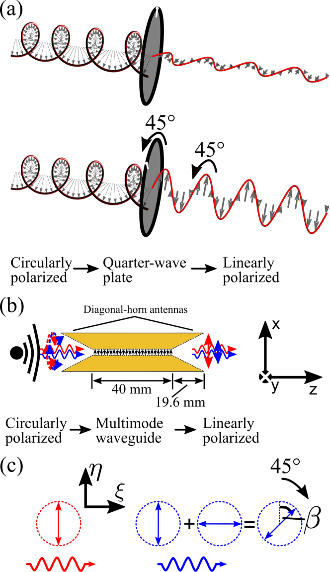
Figure 1: (a) Conventional way of transforming a left-circularly polarized electro-magnetic field into a linearly polarized field, by rotating mechanically a quarter-wave plate to the desired angle. (b) Multimode waveguide and diagonal-horn antenna assembly, acting as a non-mechanical $45^{\circ}$ polarization rotator, demonstrated in this work. The excitation of multiple waveguide modes with the circularly-polarized field, distributes the field energy equally among the waveguide modes, indicated by the red and blue photons. (c) Exciting only the fundamental waveguide mode leads to a radiated field from the output diagonal-horn antenna with a well defined linear polarization along the $\eta$-axis (co-polarization axis) of the aperture coordinate system of the diagonal-horn antenna, shown as the red photon. Further, exciting higher-order waveguide modes leads to a radiated field with a $45^{\circ}$ rotated polarization due to a superposition of linear polarizations along the $\eta$-axis and $\xi$-axis (cross-polarization axis), shown as the blue photon.

With this perspective, the polarization of the THz photon becomes a particularly interesting parameter, as it could enable THz photon entanglement experiments with the polarization being the entanglement parameter. However, in the THz domain it is a difficult task to carry out a quantitative measurement of the polarization (Fig 1(a)) without significantly disturbing the signal. The reason is, that the Rayleigh length of optical elements in the THz frequency range is usually small, i.e. only slightly larger than the beam waist, such that one often operates at the onset of beam divergence.

In the present work we aim at enhancing the toolset for THz experiments by establishing a simple method for the generation, adjusting and measurement of such a polarization.

We study in experiments and numerical simulations the polarization state of a multimode free-space sub-THz field as a function of frequency in the range from 215 to 580 GHz, that is launched from a rectangular waveguide and a diagonal-horn antenna, cf. Fig. 1(b). We present a method to measure the polarization state resulting from these multiple modes of the free-space sub-THz field using a coherent detector (photo-mixer) in combination with a planar silicon-mirror acting as a Fresnel scatterer. This enables us to determine the polarization components with high accuracy and without the need for any opto-mechanical components such as rotatable polarizers. In particular, this renders our method suitable for ultra-high frequency cQED experiments in a cryogenic environment.

We find that when only the fundamental TE₁₀ mode of the waveguide is excited, as expected, the field emitted by the diagonal-horn antenna is characterized by a predominantly linear polarization. This is consistent with our earlier findings reported in [8] whereas the emitted field still contains a cross-polarization power component of about 5$\%$. At higher frequencies we find in both simulations and experiments that excitation of higher-order modes of the waveguide (TE₂₀, TE₀₁, TE₁₁ and TM₁₁) leads to a well-defined rotation of the polarization by up to $45^{\circ}$, cf. Fig. 1(c). Despite the higher-order modes, the radiated field appears to maintain a predominant Gaussian beam character, since an unidirectional coupling to a detector was possible, whereas the unidirectionality is independent of frequency.

Section II provides the theoretical basis for the experimentally observed polarization rotation effect of the emitted THz field, starting from the waveguide theory and, eventually, describing the simulation of the near- and far-field generation of the THz field by the diagonal horn antenna. In Section III we describe various details of the experiment, including the design of the fabricated waveguide and the diagonal horn antennas, as well as the functionality of the photo-mixers. Section IV describes the measurement setup. Section V explains the measurement procedure and the method of analysis. Section VI discusses the results. Section VII concludes our work. Furthermore, we provide a detailed Appendix, comprising a description of the calibration of our setup, far-field simulations of the output field of the diagonal-horn antenna and a discussion of a single-photon detector calibration using our waveguide/diagonal-horn antenna device.

II Polarization rotation from waveguide theory and simulation

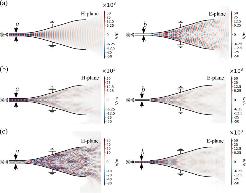
Figure 2: Near-field simulation results of the electric portion of the electro-magnetic field, expressed as electric field intensity, in the experimentally implemented antenna-feed waveguide (rectangular section with dimensions $a$ and $b$) and bell-mouthed diagonal-horn antenna shape, obtained by the CST software [27]. In the antenna-feed waveguide, which is further connected to the waveguide channel (cf. Fig. 3(b), (c) and (e)), a certain mode of the electric portion of the electro-magnetic field is excited predominantly in the H- or E-plane. After the waveguide excitation, however, an electric field develops in both planes of the diagonal-horn antenna. The electric field intensities in the diagonal-horn antenna planes are mode-dependent. The figure summarizes the results for the first three propagating modes at reasonably selected frequencies, (a) $\mathrm{TE}_{10}$ (270 GHz), (b) $\mathrm{TE}_{20}$ (480 GHz) and (c) $\mathrm{TE}_{01}$ (480 GHz). Note that the overall values of the electric field intensities, the intensities being quantified by the scales in units of V/m, in the E- and H-plane of the diagonal-horn antenna for the mode $\mathrm{TE}_{10}$, (a), are approximately swapped between same E- and H-plane for the mode $\mathrm{TE}_{01}$, (c). The overall values of the electric-field intensities in the E- and H-plane of the diagonal-horn antenna are approximately the same for the mode $\mathrm{TE}_{20}$, (b). With these three modes in superposition, polarization rotation by $45^{\circ}$ occurs around the wavevector $k_{z}$, suggested by Fig. 3(a).

The electric and magnetic field distributions in all three spatial directions ($E_{x,y,z}$ and $H_{x,y,z}$) in a rectangular waveguide are fundamentally derived as solutions of the reduced wave equations for the electro-magnetic field in the waveguide,

$$\left(\frac{\partial^{2}}{\partial x^{2}}+\frac{\partial^{2}}{\partial y^{2}}+k_{c}^{2}\right)h_{z}(x,y)=0$$ (1a)

$$\left(\frac{\partial^{2}}{\partial x^{2}}+\frac{\partial^{2}}{\partial y^{2}}+k_{c}^{2}\right)e_{z}(x,y)=0~{}.$$ (1b)

The $z$-direction is the longitudinal direction of the waveguide and the diagonal-horn antenna and at the same time the propagation direction of the electro-magnetic field in the waveguide and in the diagonal-horn antenna. Furthermore, Eq. (1a) obtains solutions for transversal electric fields for which $E_{z}=0$ and Eq. (1b) obtains solutions for transversal magnetic fields for which $H_{z}=0$. Moreover, in the above equations, $h_{z}$ fullfils the relation $H_{z}(x,y,z)=h_{z}(x,y)\exp{\left(-i\beta z\right)}$ and $e_{z}$ fullfils the relation $E_{z}(x,y,z)=e_{z}(x,y)\exp{\left(-i\beta z\right)}$. In particular, $k_{c}=\sqrt{k^{2}-\beta^{2}}$ is the cut-off wavenumber of the waveguide or a segment of the diagonal horn antenna, with $k$ being the wavevector and $\beta$ being the propagation constant.

Application of suitable boundary conditions capture the geometry of the waveguide and of the diagonal horn antenna.

Specifically, to describe the electro-magnetic field in our waveguide/diagonal-horn antenna device, eventually, makes a precise description of the transition from the waveguide to the diagonal-horn antenna necessary. This transition is a complex mechanical transition, cf. Fig. 3(e), ii and iii, which renders a precise analytical solution of the wave equation Eq. (1a) and (1b) unpractical.

Additionally, for our purposes, the description of the transition from the near- into the far-field for a multimode electro-magnetic field, emitted or received by the diagonal-horn antenna, is important for the quantitative analysis of our experimental results. For a precise evaluation of the far field of the diagonal horn antenna, the starting point would be a precisely known aperture field which could then be expanded into Gauss-Hermite functions, in order to obtain the far-field radiation pattern.

To this end, instead of a fully analytical solution, we have solved the above equations in a CST [27] simulation of the nominal waveguide and diagonal-horn antenna dimensions and shapes, since we expect from this route more precise results for our later analysis.

The near-field simulation results are shown in Fig. 2 and we specify further in Fig. 3 and Sec. III.1 the waveguide and diagonal-horn dimensions. Further, we represent E- and H-plane cuts of the electro-magnetic field in the waveguide and the diagonal horn-antenna in Fig. 2. In particular, the E- and H-plane are defined on the basis of the fundamental mode ($\mathrm{TE}_{10}$) of the waveguide, whereas the E-plane is the plane containing the electric-field vector and the H-plane is the plane perpendicular to the electric-field vector. The near-field simulation results show the projection of the electric field on the E- and H-planes, where red colors indicate an electric-field maximum and blue colors indicate an electric-field minimum, further characterized by positive and negative numbers in units of V/m. Further, since the diagonal horn antenna is much larger than the wavelength of the respective propagating modes, our simulations evaluate electric fields with several electric field maxima (red colors) and electric field minima (blue colors), shown in Fig. 2.

In general, the polarization of an electro-magnetic field is defined as the oscillation direction of the electric field component of the electro-magnetic field.

Therefore, Fig. 2(a) shows the expected result for the $\mathrm{TE}_{10}$ mode in which the electric field oscillates out of the H-plane (red colors) and into the H-plane (blue colors), therefore, the polarization is perpendicular to the H-plane and parallel to the E-plane. Note in particular the scale for the electric field in units of $\mathrm{V/m}$, shown for each simulated E- and H-plane cut of the diagonal horn antenna shape. In Fig. 2(a) the predominant electric field is established in the H-plane whereas it is approximately three order of magnitude smaller in the E-plane. This effect establishes the predominant direction of the polarization described before.

In contrast, Fig. 2(c) suggests that for the $\mathrm{TE}_{01}$ mode the polarization is perpendicular to the one of the $\mathrm{TE}_{10}$ mode. This is, like described before, evidenced by the electric field strength. This time, however, the electric field is established predominantly in the E-plane whereas it is approximately three orders of magnitude smaller in the H-plane. Since, the E- and H-planes are perpendicular to each other, also the polarization in the $\mathrm{TE}_{01}$ is perpendicular to the polarization of the $\mathrm{TE}_{10}$ mode. Once these two modes propagate simultaneously, the effective polarization is the vector sum of the two polarizations of the modes, hence, the polarization is rotated by $45^{\circ}$.

In particular, we show in Appendices C and D that the far-field shows corresponding features. This is an important aspect since the far-field is coupled to our detection scheme.

The described effects are the fundamental basis of our experimentally observed polarization rotation by $\sim 45^{\circ}$.

Additionally, the higher order modes $\mathrm{TE}_{20}$, $\mathrm{TE}_{11}$ and $\mathrm{TM}_{11}$ result in essentially near-field patterns of the like shown in Fig. 2(b). Here, the near-field shows a fundamentally different pattern compared to the ones in Fig. 2(a) and (c). At a given longitudinal position, on one side of the symmetry axis of the diagonal-horn antenna, a maximum or minimum electrical field is obtained whereas on the other side of the symmetry axis at the same longitudinal position, a respective opposite field is found. Additionally, the field intensities in the H- and E-plane are practically equal. This means that the effective polarization would be zero when averaged over the diagonal-horn aperture. Near-field effects of this kind, essentially a capacitive effect due to the confined geometry of the diagonal-horn antenna and the waveguide, are known to vanish in the far-field. In the far-field, equal amounts of power are then obtained in the co- and cross-polarization components of the diagonal horn antenna, like we describe in Appendices C and D together with far-field simulation results shown in Figs. 8(c) and (d) for the $\mathrm{TE}_{20}$ mode. The equal power components in the co- and cross-polarization components of the far-field of the diagonal horn antenna for the modes $\mathrm{TE}_{20}$, $\mathrm{TE}_{11}$ and $\mathrm{TM}_{11}$, lead to individual propagating fields with $\sim 45^{\circ}$ rotated polarization. When all five modes propagate, a superposed electro-magnetic field is obtained, being characterized by the aforementioned rotated polarization.

Importantly, for the far-field we studied in our simulations the higher-order propagating modes in the waveguide and the created multimode (in our case up to five) electro-magnetic field. Interestingly, we have discovered that this field is characterized by co- and cross polarization components of the electric field which are practically in-phase in the same mode, when radiated from the diagonal-horn antenna into free space. Furthermore, our multimode simulations find that the phase-delay between the aforementioned far-field (i.e. free space) electric fields in different modes is practically negligible as well. This means, that the different modes are emitted by the diagonal-horn antenna in a coherent fashion and are practically not time-delayed with respect to each other. This is key for an effective polarization rotation of $45^{\circ}$ to happen and for generating a coherent electric field with a predominant linear polarization content and with a negligible circular polarization content.

III Experimental system

III.1 Waveguide assembly

In order to test the aforementioned prediction, our starting point is a machined diagonal-horn antenna and waveguide assembly as shown in Fig. 3(a), suitable for the frequency range from 215 to 580 GHz. Similar units are commonly used in mixer-assemblies for heterodyne detection in astronomical instruments (see for example de Graauw, Th. et al. [28]). It is made from the material CuTe, with waveguide dimensions (Fig. 3(c) and (e)) of $a=800~{}\mu\mathrm{m}$ and $b=400~{}\mu\mathrm{m}$. At each end a diagonal-horn antenna is attached with the feedpoint of the two antennas matching the waveguide dimensions.

Figure 3(a) shows a completed unit and a representation of an emitted electro-magnetic field. The diagonal horn can be disassembled into two halves along its E-plane (Fig. 3(b)), which reveals its dimensions as defined in Fig. 3(d). The dimensions in Fig. 3(d) of the diagonal-horn antenna aperture (left) and the profile (right) are $w_{A}=9.9~{}\mathrm{mm}$ (geometric aperture-width), $l=7~{}\mathrm{mm}$ (geometric aperture edge-length), $w_{F}=400~{}\mu\mathrm{m}$ (waveguide feed, $b$-side, $L_{F}=19.6~{}\mathrm{mm}$ (feed length), $L_{P}=21.48~{}\mathrm{mm}$ (profile length) and $w_{C}=4.91~{}\mathrm{mm}$ (width of the horn profile at distance $L_{F}/2$ from the feedpoint).

The cross-sections shown in Fig. 3(e) picture the electro-magnetic field of the fundamental $\mathrm{TE}_{10}$-mode in the waveguide (Fig. 3(b) and (c)) at position i, and in the diagonal-horn antenna aperture at position iv. In the last panel of Fig. 3(e), we depict the aperture coordinates $\eta$ and $\xi$, already introduced in Fig. 1(c). The co- and cross-polarizations point in direction of $\eta$ and $\xi$.

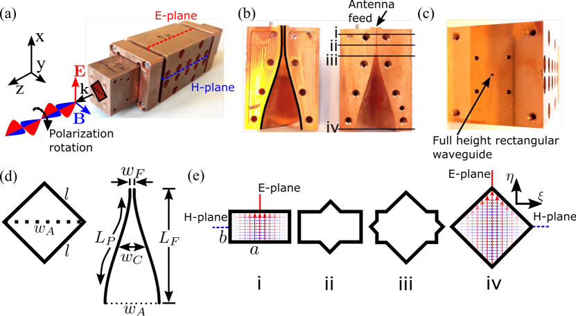
Figure 3: Design, components and assembly of the fabricated diagonal-horn antenna and waveguide device. (a) The completed assembly, diagonal-horn antennas opened along the E-plane (b) which are connected by a full-height rectangular waveguide (c). In (b), left: the black profile emphasizes the antenna profile. Right: subdivision into cross sections (i)-(iv), shown in more detail in (e). (d) Cross-sections of the diagonal-horn antenna aperture (left) and the profile (right). (e) Cross-sections indicated in (b), showing the inner conductor-shape of the waveguide and the diagonal-horn antenna, with the electro-magnetic field of the fundamental $\mathrm{TE}_{10}$-mode in the waveguide and diagonal-horn antenna at positions i and iv. The $\eta$-$\xi$ aperture coordinate system is shown in iv.

The signal path in our setup is as follows. The input diagonal-horn antenna receives an electro-magnetic sub-THz field generated by a photo-mixer, exposed to the signal of two coupled DFB lasers. This signal excites the waveguide with the multimode field. Subsequently, the waveguide excites the output diagonal-horn antenna which then emits a multimode electro-magnetic field into free space where it gets reflected from the planar silicon-mirror towards a coherent detector, where it is detected and analyzed.

III.2 Photo-mixers

To build the foundation for a better understanding of our experiments, we will describe in more detail the way of operation of the photo-mixers by means of our experimental setup, shown in Fig. 4. The frequency-tunable electro-magnetic signal, in the frequency range of 215 to 580 GHz, is generated and detected by superimposing the outputs of two 780 nm distributed feedback (DFB) lasers in a beam combiner (BC) and shone on two GaAs photo-mixers connected at the output of the beam combiner via polarization maintaining fibers (PMF). One photo-mixer acts as coherent sub-THz source (S) and the second acts as a coherent sub-THz detector (D) [29]. The incident laser power on each photo-mixer is approximately $30~{}\mathrm{mW}$. The desired frequency of the sub-THz electro-magnetic field is set by adjusting the difference frequency, $f$, between the two DFB lasers. Optimal coupling between all optical elements is achieved by arranging the set-up in such a way that the propagating Gaussian beam-divergence is minimized and a narrow beam hits the detector.

The planar-silicon mirror at the output makes it possible to measure the polarization by using Fresnel scattering, to be discussed below, without using any movable parts and with a minimal number of optical components.

IV Measurement Setup

The polarization rotation is measured based on the principle of Fresnel scattering, implemented by the scattering of the electro-magnetic field from a silicon mirror, cf. Fig. 4. The scattered field is received by the detector with different signs, because either the positive or negative region of the electro-magnetic field oscillation reaches the detector area first. Equivalently, this corresponds to a phase shift of $\pi$ of the electro-magnetic field which depends on the linear polarization of the field, according to the Fresnel theory [30]. The sign is measured directly in our coherent detection scheme, since it determines the dc-photocurrent direction.

The signal is detected by coherent detection of the scattered electro-magnetic field, which contains the phase information for the two different waveguide orientations (cf. caption of Fig. 4), which we adjust in two successive measurements. The phase information of the detected field is extracted by post-processing the frequency-dependent transmission data between source and detector in Fig. 4 by means of a Hilbert transformation [31, 8], described below. In this way we build the basis for the evaluation of the phase-phase correlation function [Eq. (4)] for the two different waveguide orientations.

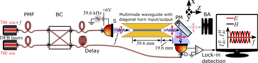
Figure 4: Measurement system to measure the polarization at the output of the diagonal-horn antenna. Coherent sub-THz source (S) and detector (D) are used and the lock-in detected signal is displayed as a function of frequency. The planar silicon-mirror (PM, TYDEX [32]) acts as a Fresnel scatterer and enables the polarization measurement. It reflects linearly-polarized electric fields with polarization components parallel and perpendicular to the plane of incidence (paper plane), with opposite signs (and slightly different magnitudes) into the aperture of the coherent detector. Two successive measurements result in the detector currents $I_{dc}^{E}$ and $I_{dc}^{H}$, Eqs. (3a) and (3b), when the E- and H-plane of the waveguide (cf. Fig. 3) and diagonal-horn antenna are successively aligned parallel to the plane of incidence. This implements a direct measurement of the correlation function in Eq. (4). A beam absorber (BA) attenuates a standing wave in the setup.

Two details are important in the interpretation of our measurement results. First, the direction of the current flow in the detector. The dc-photocurrent $I_{dc}$ is periodic with the detuning frequency $f$ and dependents on the delay length $\Delta L=L_{S}+L_{0}-L_{D}$ between the optical fibers, including the free space path of the sub-THz field from the source to the detector [31]. $L_{S}$ and $L_{D}$ are the (different) optical path lengths travelled by the two superimposed DFB laser fields to the source and detector through the optical fibers. The length $L_{0}$ is the additional path length, travelled by the sub-THz field from the source to the detector through free space, through the diagonal horns and through the waveguide (black wiggly and dashed arrows in Fig. 4).

Secondly, the sign and the magnitude of $I_{dc}$ is also determined by two more sets of parameters related to the Fresnel scattering effect. The first parameter set is the sign and the absolute value of the Fresnel amplitude reflection coefficient, $r^{\perp,\parallel}(f)$, of the electro-magnetic field at the output of the planar silicon-mirror, where the electric field component has a polarization perpendicular to ($\perp$) or/and parallel ($\parallel$) to the planar silicon-mirror plane of incidence. Furthermore, the sub-THz electro-magnetic field has a well defined phase $\varphi^{\perp}$ or $\varphi^{\parallel}$ for each of the two polarizations. Generally, these phases dot not have the same values, but are in practice not much shifted with respect to each other. The second parameter is the amplitude of the electric component, contained in the two polarization components perpendicular ($\perp$) and/or parallel ($\parallel$) with respect to the planar silicon-mirror plane of incidence. In this work it is sufficient to determine the phases of the output field for two different orientations of the waveguide.

The polarization angle of the output field of the diagonal-horn antenna follows now from a statistical analysis by means of a phase-phase correlation function [Eq. (4)]. The idea is that the phase of the output field after scattering from the planar silicon-mirror into the detector differs by a shift of exactly $\pi$ between the two successive measurements, which signals the detection of pure $\perp$- and $\parallel$-components. This $\pi$-shift of the phase is well known and described by the Fresnel theory [30], but it should be supplemented with another phase shift due to the finite thickness of the planar silicon-mirror. For the real-valued detector currents $I_{dc}(f)$, flowing in response to a detected electro-magnetic field of frequency $f$, the analytical complex-valued detector current reads

$$\mathcal{I}_{dc}(f)=I_{dc}(f)+i\mathcal{H}\left[I_{dc}(f)\right]=S(f)\exp\left[i\phi(f)\right]~{}.$$ (2)

Here, $\mathcal{H}(\cdots)$ is the Hilbert transformation [33], $\phi(f)$ the instantaneous phase of the signal and $S(f)$ is the instantaneous amplitude. For the rest of the paper, $\phi(f)$ is the key observable from which we derive our results, explained in more detail below.

A phase shift deviating from $\pi$, eventually, resulting in phase jumps in the detector, is expected for an output field characterized by a mixture of $\perp$- and $\parallel$-components. We explain this case in more detail in the following paragraph, in particular the case of an equal mixture of $\perp$- and $\parallel$-components, hence, an output field with $45^{\circ}$ rotated polarization.

V Measurement procedure and method of analysis

V.1 Obtaining the data

The sub-THz electric field component received by the detector leads to an ac-voltage drop across an interdigitated capacitor part of the detector with a frequency equal to the difference in laser frequencies $f$. Together with the laser-induced impedance modulation at the same frequency, but in general with a different phase, a coherent dc-photocurrent, $I_{dc}(f)$, flows in the positive or negative direction (dependent on the phase) across the feedpoint of the log-spiral circuit. We detect this dc-photocurrent with a post-amplification scheme described in [8], with each data point integrated over 500 ms. This detection scheme resembles a coherent detector at sub-THz frequencies with a high-dynamic range up to 80 dB [29] like described by Roggenbuck et al. [31]. A beneficial aspect of this scheme is that it measures the transmitted amplitude rather than only the transmitted power. This allows us to use the planar silicon-mirror in our setup as a Fresnel scatterer.

We perform our measurements in two successive steps. First, we align the waveguide and diagonal-horn antenna with the E-plane parallel to the plane of incidence and, secondly, we align them with their H-plane parallel to the plane of incidence. For each of these steps we record the detector current (given in analytical form in Eqs. (3a) and (3b)) as a function of frequency, covering the range of 215 GHz to 580 GHz. For the fundamental waveguide mode up to a frequency of about 400 GHz, determined by the diagonal-horn antenna and the rectangular waveguide geometry [8], the polarization is predominantly parallel to the E-plane. By rotating the rectangular waveguide and diagonal-horn antenna by 90 degrees, we also rotate the polarization by the same amount. By adding the planar silicon-mirror to the setup described in [8], we obtain the polarization sensitive coherent detector.

In the measurement situation in which the rectangular waveguide and diagonal-horn antenna assembly is aligned such that the E- or H-plane is parallel to the silicon-mirror plane of incidence, we can express the detector currents as,

$$I_{dc}^{E}(f) =\mathcal{C}\sum_{l}\mathcal{A}\cdot\mathrm{Re}\left[r^{\parallel}(f)\right]\mathcal{E}_{l}^{E}\cos\left[\frac{2\pi f\Delta L}{c_{0}}+\varphi^{\parallel}_{l}+\Delta\varphi^{\parallel-\perp}_{l}\right]C^{(1)}_{l}(f)+\mathrm{Re}\left[r^{\perp}(f)\right]\mathcal{E}_{l}^{H}\cos\left[\frac{2\pi f\Delta L}{c_{0}}+\varphi^{\perp}_{l}\right]C^{(2)}_{l}(f)~{},$$ (3a)

$$I_{dc}^{H}(f) =\mathcal{C}\sum_{l}\mathrm{Re}\left[r^{\perp}(f)\right]\mathcal{E}_{l}^{E}\cos\left[\frac{2\pi f\Delta L}{c_{0}}+\varphi^{\parallel}_{l}\right]C^{(3)}_{l}(f)+\mathcal{A}\cdot\mathrm{Re}\left[r^{\parallel}(f)\right]\mathcal{E}_{l}^{H}\cos\left[\frac{2\pi f\Delta L}{c_{0}}+\varphi^{\perp}_{l}+\Delta\varphi^{\parallel-\perp}_{l}\right]C^{(4)}_{l}(f)~{}.$$ (3b)

The amplitudes $\mathcal{E}^{E,H}_{l}$ quantify the field strength in the E- or H-plane for a given mode $l\in\{0\ldots 5\}$ (for more details cf. Appendix C and D). Up to a constant they fully determine the size of the detector current. When multiplied with the Fresnel scattering amplitudes $r^{\parallel,\perp}$ and up to a propagation factor and the polarization orientation in free space, the resulting expression is equivalent to free space propagating fields $\boldsymbol{\mathcal{E}}_{\parallel}$ or $\boldsymbol{\mathcal{E}}_{\perp}$. Furthermore, $c_{0}$ is the velocity of light in vacuum and $\mathcal{C}=dZ_{0}/2Z_{det}^{2}\approx 1\cdot 10^{-12}\mathrm{-}1\cdot 10^{-13}~{}\mathrm{m/\Omega}$ is the coupling constant between the free space electro-magnetic field and the detector which we assume to be the same for the $\parallel$- and $\perp$-components. Once the detector is fixed on the optics table and its position cannot be optimized anymore for maximal response, the coupling to the detector will be different for the $xz$- and the $xy$-plane due to imperfections of the detector. We account for this asymmetry by the constant $\mathcal{A}=0.85$, which we determine experimentally by measuring the Fresnel amplitude reflection coefficients for the $\perp$- and the $\parallel$-components (for more details cf. Appendix B).

The real part of each Fresnel amplitude reflection coefficient in Eqs. (3a) and (3b) contributes in two ways to the measured dc-photocurrent. First, it evaluates the sign (or equivalently the phase shift) of the scattered wave and, second, it quantifies the frequency dependent reflection of the electro-magnetic field from the planar silicon-mirror.

The argument of the cosine, $2\pi f\Delta L/c_{0}$, describes the frequency periodicity of the detected field when it arrives with a certain time delay $\Delta L/c_{0}$ at the detector, as described before. The phase shifts of the detected polarization components, $\phi^{\parallel,\perp}$, add in a similar fashion to the argument of the cosine. In our modeling we equate the phase difference between the in Sec. VI.1 further discussed co- and cross-polarizations with $\phi^{\parallel}$ while setting $\phi^{\perp}=0$. Further details are shown in Fig. 9(b) and (d) of Appendix D.

We account also for the imaginary part of the Fresnel amplitude reflection coefficients upon scattering from the planar silicon-mirror by evaluating their difference in phase shift between $\parallel$- and $\perp$-components, $\Delta\phi_{l}^{\parallel-\perp}$. The fundamental reason for this extra phase shift is the finite thickness of the planar silicon-mirror which imposes different phase shifts on the $\parallel$- and $\perp$-components when scattered to its output.

Finally, the current correction coefficients $C^{i}_{l=0}(f)=1$ (single mode) and for $l>1$ (multiple modes), $C^{i}_{l}(f)\in[0,1]$ are unknown. Nevertheless, these coefficients shall provide the basis for corrections to the detector current. Such a correction seems necessary, because for the case $l>1$, multiple currents flow in parallel in the active detector area while one measures only the resulting (sum) effective current. In the standard photo-mixer theory, the theoretical framework of multiple-mode detection is not largely discussed and no solution seems to be prepared so far.

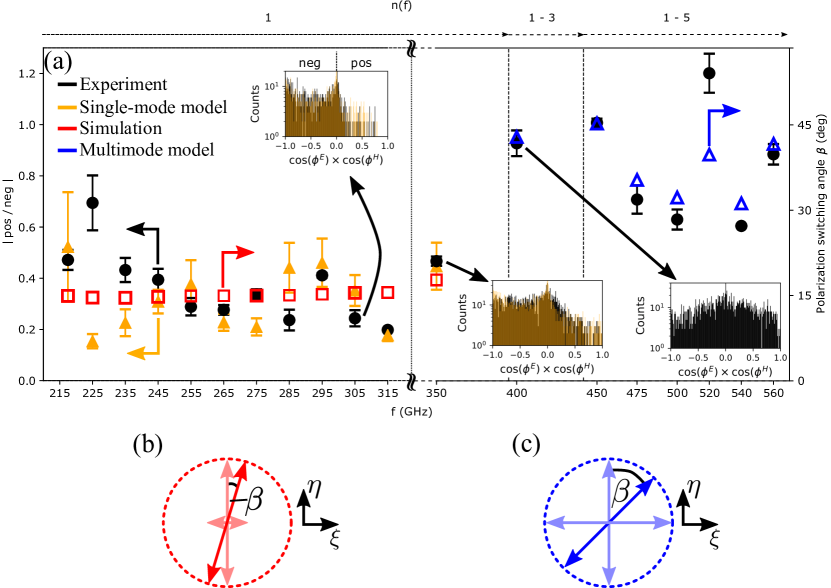
Figure 5: Overview of the results on the measured polarization of the rectangular waveguide and diagonal-horn antenna assembly over the frequency range from 215 to 580 GHz. The line at the top indicates the presence of the number of higher order modes. Note the scale change at 315 GHz. Panel (a) Experimental (black) and simulation (red) results together with results for the single-mode (orange) and multimode (blue) model. The experimental data-points (black) are evaluated from histograms like shown in the inset, by dividing the positive counts by the negative ones, pos/neg (left y-axis). The black-colored histograms contain the experimental values of the instantaneous phase-phase correlation function for the output electro-magnetic field, $\cos(\phi^{E})\times\cos(\phi^{H})$ (Fig. 4 and Eq. (4)).

V.2 Data analysis

In order to extract the polarization content from the measured detector responses, contained in the phases of Eqs. (3a) and (3b), we need to perform a statistical analysis on these instantaneous phases by means of correlation functions. The Hilbert transformation, Eq. (2), evaluates the instantaneous phases $\phi^{E}(f)$ or $\phi^{H}(f)$. Each of these phases as a function of frequency can be selected by orienting the rectangular waveguide and diagonal-horn antenna assembly with its E- or H-plane parallel with respect to the silicon-mirror plane of incidence.

In the experimental data, the origin of instantaneous phase values and most dominant contributions are hidden. However, from Eqs. (3a) and (3b) a number of different contributions to the phase shift are obvious. The most dominant terms are of the form $\mathrm{Re}\left[r^{\parallel,\perp}(f)\right]\mathcal{E}_{l}^{E}$ and $\mathrm{Re}\left[r^{\parallel,\perp}(f)\right]\mathcal{E}_{l}^{H}$ and are the ones which are due to the Fresnel scattering. Finally, a correlator of the form

$$C\left(\phi^{E},\phi^{H}\right)=\cos\left(\phi^{E}\right)\times\cos\left(\phi^{H}\right)~{},$$ (4)

yields the phase-phase correlation function of the instantaneous phases. In particular, Eq. (4) evaluates to ’1’ when the instantaneous phases of the E- and H-plane are in-phase and it evaluates to ’-1’ when they are out-of-phase, i.e. shifted by $\pi$ with respect to each other. Such a shift is expected for an ideal linear polarization due to the Fresnel scattering. Continuous values between ’1’ and ’-1’ are possible as well and quantify some extra phase shifts which can occur. These extra phase shifts have as a source the terms $\varphi_{l}^{\parallel,\perp}$ and $\Delta\varphi^{\parallel-\perp}$ in Eqs. (3a) and (3b). They are usually small, i.e. influencing the measurement results only in a range smaller than the error bars in Fig. 5, compared to a more dominant effect, occurring when two similarly large orthogonal polarizations scatter off the planar silicon-mirror and are detected at the same time. This drives positive as well as negative detector currents (cf. Appendix A) which tend to cancel each other, leading to phase jumps and continuous correlator values between ’1’ and ’-1’. This is also the expected experimental signature of the $45^{\circ}$ linear-polarization rotation, cf. Fig. 1(c). For the case of a linear polarization, containing just a small cross-polarization component, one expects a different distribution of correlator values ’1’ and ’-1’ compared to a $45^{\circ}$ linear-polarization rotation. In the former case, mostly values of ’-1’ should be obtained because of the smallness of the cross-polarization component. We confirm this outcome consistently in our experiment.

It is beneficial to understand the experimental data, by evaluating the correlator in Eq. (4) over a meaningful frequency bandwidth in the measured frequency range. For measurements exciting only the fundamental $\mathrm{TE}_{10}$ mode, we evaluate the correlator over a bandwidth of 10 GHz to obtain a single data-point and for measurements which excite higher-order modes, we have chosen a bandwidth of 20 GHz. Through this choice a large enough sample of correlator values can be used to compare with the theoretical model. In addition, it has proven to be convenient to quantify the correlator by plotting its values in a histogram, as shown in Fig. 5.

VI Discussion of the results

In our experiment, we have measured the multimode field from the output diagonal-horn antenna through the detector currents $I_{dc}^{E}(f)$ and $I_{dc}^{H}(f)$ as a function of frequency. The detector currents are modeled by the analytical form of the Eqs. (3a) and (3b). The statistical analysis of the detector currents leads to histograms like shown in the inset of Fig. 5(a). They contain the value distribution of the phase-phase correlation function, Eq. (4). In a next step we sum over the positive and negative counts in the histograms and build the quotient pos/neg. This is shown as the black data-points which refer to the left part of the y-axis in Fig. 5(a).

In order to relate this measurement to the polarization angle $\beta$ (shown in Fig. 5 and also in Fig. 1(c)), we combine our measurements with electro-magnetic field simulations of the radiation pattern from the exact diagonal-horn antenna geometry. From these simulations, we obtain the electric-field strengths $\boldsymbol{\mathcal{E}}_{\eta}$ and $\boldsymbol{\mathcal{E}}_{\xi}$, which the diagonal-horn antenna radiates into the far-field with the rectangular waveguide acting as the excitation source. The polarization angle is given by

$$\beta=\arctan{\left(\boldsymbol{\mathcal{E}}_{\xi}/\boldsymbol{\mathcal{E}}_{\eta}\right)}~{}.$$ (5)

We use the computer-aided 3D mechanical design of the diagonal-horn antenna to model the exact antenna geometry in the electro-magnetic field simulation software CST [27].

VI.1 Fundamental $\mathrm{TE}_{10}$ mode

First, we discuss the results for the fundamental $\mathrm{TE}_{10}$ mode and address later the multimode case. When exciting in the simulation this mode, propagating over the range from 180 GHz to 360 GHz, we obtain at each selected frequency a set of electric-field strengths $(\boldsymbol{\mathcal{E}}_{\eta},\boldsymbol{\mathcal{E}}_{\xi})$. They quantify the far-field radiation pattern and through this also the direction of the polarization, illustrated in Fig. 5(b). This is shown as the red data points in Fig. 5(a), which are consistent with a 5% cross-polarization power component of the diagonal-horn antenna. For more details on the frequency dependence of the cross-polarization we refer to Fig. 9(a) of Appendix D. Note that the field strengths $(\boldsymbol{\mathcal{E}}_{\eta},\boldsymbol{\mathcal{E}}_{\xi})$ refer to the aperture coordinate system of the diagonal-horn antenna, i.e. they are fixed to the frame of reference of the diagonal-horn antenna and have to be distinguished from the components $(\boldsymbol{\mathcal{E}}_{\parallel},\boldsymbol{\mathcal{E}}_{\perp})$, which refer to the planar silicon-mirror plane of incidence. More details are given in Appendix D. Since the simulation results $(\boldsymbol{\mathcal{E}}_{\eta},\boldsymbol{\mathcal{E}}_{\xi})$ are complex valued, we also obtain the phase information of the orthogonal field components. For more details on the frequency dependence of this phase we refer to Fig. 9(b) of Appendix D. Together with the electric-field strength we, therefore, fix for the detector currents every free parameter in Eqs. (3a) and (3b). Finally, by substituting the values obtained from the simulation in the $\eta\textrm{-}\xi$ aperture coordinate system into Eqs. (3a) and (3b), we need to determine which field component lies in the E- or H- plane. For the $\mathrm{TE}_{10}$ mode, the principal field direction is along the E-plane. Consequently, $\lvert\boldsymbol{\mathcal{E}}_{\eta}\rvert\widehat{=}\mathcal{E}^{E}$, $\lvert\boldsymbol{\mathcal{E}}_{\xi}\rvert\widehat{=}\mathcal{E}^{H}$ and corresponding substitutions hold for the phases. A Hilbert transformation of the obtained Eqs. (3a) and (3b) provides the instantaneous phases $\phi^{E}$ and $\phi^{H}$ and the correlator $C(\phi^{E},\phi^{H})$, Eq. (4). By this procedure we obtain the orange-colored histograms and data points in Fig. 5(a). In order to obtain the latter, we sum again over the positive and negative counts in the model histograms.

An exact match with the experimental data is not obtained, which is not surprising given the complexity of the experiment. However, the key features are correctly described by our model. For the frequencies 285 GHz to 350 GHz, the trend of the data is correctly predicted and the absolute values of the experiment and the single-mode model are close to each other. In the frequency range 245 GHz to 275 GHz, a comparable trend of the model and the experiment is not evident, but the absolute values are again close to each other. Furthermore, the obtained orange-colored model histograms compare sufficiently well to the black-colored experimentally determined histograms.

In particular, we like to highlight the matching shapes between the experimentally determined histograms and the model histograms at 305 GHz and 350 GHz. The histogram at 305 GHz shows predominantly negative values of the correlator $C(\phi^{E},\phi^{H})$. This is indicative of a predominantly linearly polarized electro-magnetic field, as explained in Sec. IV and Sec. V.2. Moreover, a distribution of negative values and a few positive values is obtained for the correlator. This signifies that a small cross-polarization component is contained in the electro-magnetic field and that the co- and cross-polarization are (slightly) phase shifted with respect to each other. In contrast, a perfectly linearly-polarized electro-magnetic field without cross-polarization content would result in single correlator values of ’-1’. Compared to the histogram at 305 GHz, the histogram at 350 GHz shows a softened edge around the correlator value ’0’, extending into the positive-value domain of the histogram. This is due to the onset of the multimode propagation and the incipient polarization rotation, leading to measured phase jumps in the detector current, as explained in Sec. V.2. The experimental data corresponding to the lowest frequencies are not correctly described by the model. This is most likely due to the Gaussian beam profiles of the photo-mixer which become non-ideal at these frequencies. In addition, we expect an influence from the vicinity of the propagation cut-off of the diagonal-horn antenna at about 180 GHz. The error bars quantify a small but measurable phase drift during the measurement.

VI.2 Higher-order modes

Higher-order modes propagate in the waveguide from frequencies of $\approx 360$ GHz upwards. The total number of propagating modes is counted by the mode index $n(f)$ in Fig. 5(a). Our multimode simulations excite at selected frequencies all possible, i.e. energetically allowed, higher-order modes and through this we obtain, like before, sets of electric fields $(\boldsymbol{\mathcal{E}}_{\eta},\boldsymbol{\mathcal{E}}_{\xi})$. We find in this case that the electric fields in the $\eta$- and $\xi$-direction are approximately of equal magnitude, cf. Fig. 9(c) and Appendix D. As a result of this, the polarization angle changes from $\beta\approx 15^{\circ}$ ($\mathrm{TE}_{10}$ mode) to $\beta=45^{\circ}$, cf. Fig. 5(c). The signature for this effect in the experiment are continuous correlator values between ’1’ and ’-1’, resulting in histograms of the type shown in Fig. 5(a) at 400 GHz. Here, the histogram is characterized by balanced positive and negative values, consistent with the prediction of Sec. V.2. Accordingly, the quotient of the sum over the positive and negative counts in the histogram, ${\it pos/neg}\rightarrow 1$. We further find in far-field simulations that the phase difference between the $\eta$- and $\xi$-components of the electric fields of the same mode is negligible, cf. Fig. 9(d) of Appendix D, and similarly the phase differences between the electric-field components of different modes. Based on this, a simple multimode model can be established in which the quantity ${\it pos/neg}$ ratio directly relates to the polarization angle $\beta$. If ${\it pos/neg}=1$, then $\beta=45^{\circ}$ and if ${\it pos/neg}$ is smaller or larger than one, the polarization angle equals either $\arctan({pos/neg})$ or $\arctan({neg/pos})$. The latter indetermination of the polarization angle is due to the measurement procedure in which we rotate the waveguide by $90^{\circ}$, to measure the currents $I_{dc}^{E}$ and $I_{dc}^{H}$. Therefore, if ${\it pos/neg}$ is not exactly equal to one, we cannot quantify whether the polarization direction was slightly larger or smaller than $45^{\circ}$. The blue data points in Fig. 5(a) show the evaluation taking $\arctan({pos/neg})$. The other case is obtained by mirroring the blue data points with respect to $45^{\circ}$.

VII Conclusion

To conclude, we have shown that a diagonal-horn antenna, connected to a full-height rectangular waveguide, emits a linearly polarized electro-magnetic field, if the rectangular waveguide is excited by the $\mathrm{TE}_{10}$ mode. To confirm the field polarization experimentally we have used a method based on only a coherent detector and a planar silicon-mirror, acting as a Fresnel scatterer. This scheme is compatible with cryogenic experiments. At higher frequencies, we find that a multimode electro-magnetic field in the rectangular waveguide induces a polarization rotation by about $45^{\circ}$ of the emitted field from the diagonal-horn antenna, as confirmed by our simulations. The source of this polarization rotation is an advantageous mode topology in the rectangular waveguide.

Appendix A Measured detector response roll-off for a multimode sub-THz field

Once the multimode sub-THz field is excited in the diagonal-horn antenna and is radiated from its aperture into free space, it consists of two fields, $\boldsymbol{\mathcal{E}}_{\parallel}$ and $\boldsymbol{\mathcal{E}}_{\perp}$, having equal magnitudes and polarizations perpendicular to each other. The resulting polarization direction is the vector sum of the polarizations of the two fields and is, hence, $45^{\circ}$ rotated compared to the polarization of the fundamental $\mathrm{TE}_{10}$ mode. Detecting the superposition of the two fields $\boldsymbol{\mathcal{E}}_{\parallel}$ and $\boldsymbol{\mathcal{E}}_{\perp}$, drives positive as well as negative currents in our coherent detector, that ideally exactly cancel each other. A signature of this effect would be a faster decrease of the detector current than one would expect due to its intrinsic roll-off. We measured the latter roll-off by a transmission measurement between source and detector only.

In a first step, we have positioned the source and detector face-to-face and adjusted the distance between their apertures such that their beam waists lie on top of each other. By this we ensure maximum coupling between source and detector.

In a second step, we have measured the detector response as a function of frequency between 150 GHz and 320 GHz. A Lorentzian curve of the form $A_{0}/\left[1+(2\pi f\tau)^{2}\right]$, with time constant $\tau=500$ fs and $A_{0}$ a constant, fits the envelope of the detector response, $\tau$ being equal to the detector roll-off time. When comparing this intrinsic detector roll-off with the roll-off induced by the multimode field in the same detector, shown in Fig. 6(a), we find that the latter decays faster. This is in-line with inducing positive as well as negative currents which, at least partly, tend to cancel each other. This effect leads primarily to phase jumps, shown in Fig. 6(b), caused by suppressing the total detector current due to the multimode field.

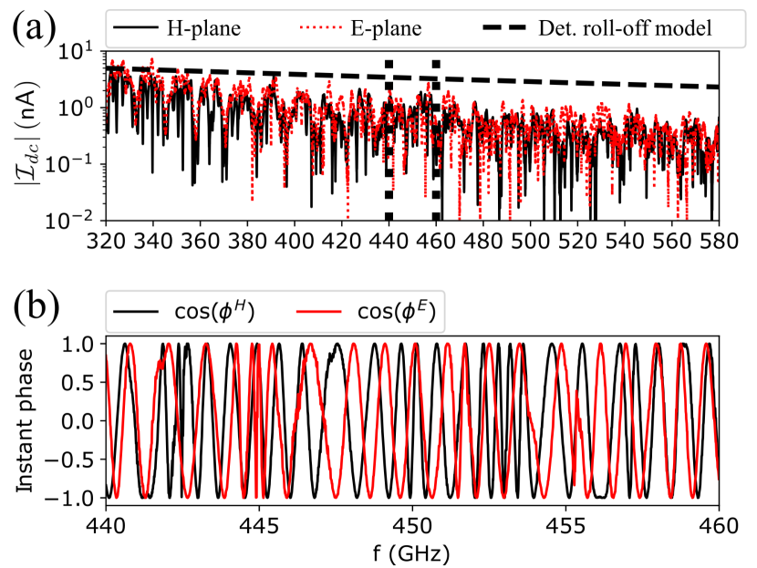
Figure 6: Detected multimode sub-THz field scattering off the $45^{\circ}$-tilted silicon mirror. (a) Measured detector response roll-off, expressed by $\lvert\mathcal{I}_{dc}\rvert$, Eq. (2) of the main text. The black and the red trace show measurements when the H- or E-plane of the diagonal-horn antenna and waveguide are aligned parallel to the planar silicon-mirror plane of incidence. Note that the fluctuations of $\lvert\mathcal{I}_{dc}\rvert$ are due to the planar silicon-mirror transmission/reflection and partly also due to standing waves, but are not caused by the noise of the detector. The dashed line shows the measured Lorentzian detector response with roll-off time constant of 500 fs, determined by a transmission measurement between source and detector only. (b) Phase of the detected sub-THz field within a selected frequency range (dotted lines in (a)). Due to the detected multimode field, it shows phase jumps compared to the more ordered phase as a function of frequency in Fig. 7(b) where only a single mode is detected. The data in the shown frequency window in (b) is employed to determine the datapoint at 450 GHz in Fig. 5(a) of the main text.

Appendix B Detection asymmetry $\mathcal{A}$ of parallel and perpendicular polarization components

An ideal detector couples equally strong to the $\parallel$- and $\perp$-components of a received sub-THz field. In this case, one measures directly and only up to a coupling constant the Fresnel scattering amplitudes.

We evaluate the frequency dependence of these amplitudes, $r^{\parallel}(f)$ and $r^{\perp}(f)$, using the Fresnel theory applied to the planar silicon-mirror. The mirror is characterized by the refractive index $n=3.416$ and a thickness of $t=3.415$ mm. For calibration purposes, we measured the amplitude reflection coefficients using the same coherent detector setup as described in the main text and confirmed their theoretically evaluated frequency dependence, cf. Fig. 7(a). Furthermore, we find also the expected Fabry-Perot resonance condition of the planar silicon-mirror which fully transmits the signal into the beam dump (element labeled ’BA’ in Fig. 4 of the main text) at frequencies $pc_{0}/[2nt\cos\left(\alpha\pi/180\right)]$, with $p$ being an integer and $\alpha=45^{\circ}$ is the angle of the planar silicon-mirror with respect to the axis of propagation of the input field. For these frequencies, both amplitude reflection coefficients are equal to zero.

We conducted this experiment and compared it to theory, in order to identify a possible asymmetry in the coupling to the $\parallel$- and $\perp$-components which we need to take into account in our modeling procedure. We find by this comparison that our detector couples to the $\parallel$-field component slightly stronger than to the $\perp$-field component. In order to compensate for this asymmetry, we need to multiply a factor $\mathcal{A}=0.85$ to the experimentally determined $\parallel$-component of the scattering amplitude to match it to the theoretical prediction.

In a second step we obtained the phases $\phi^{E}$ and $\phi^{H}$ after measuring the detector currents $I_{dc}^{E}$ and $I_{dc}^{H}$. Note the close to ideal phase shift of $\pi$ between the black and red trace in Fig. 7(b) which show the cosine of the respective phases. This is also predicted by the Fresnel theory for the scattering of parallel and perpendicular polarizations off a dielectric layer. Deviations from the ideal phase shift condition are evident in our measurement as well and occur due to a number of reasons. First, a finite amount of cross-polarization in the detected beam, second, a relative phase shift (though being tiny) between co- and cross-polarizations and, third, the finite thickness $t=3.415$ mm of the planar silicon-mirror which changes the relative phase shift between the reflected parallel and perpendicular components of the sub-THz wave, $\Delta\varphi^{\parallel-\perp}$, in Eqs. (3a) and (3b) of the main text.

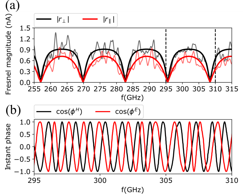
Figure 7: Detected single-mode sub-THz field scattering off the $45^{\circ}$-tilted silicon mirror. (a) Measured Fresnel magnitude of a detected free-space sub-THz field, being excited by the waveguide $\mathrm{TE}_{10}$ mode and radiated into free-space by the diagonal-horn antenna. (b) Measured instantaneous phase $\phi^{H,E}$, after scattering off the planar silicon-mirror. In (a) the smooth thick lines show the Fresnel theory and are compared with the experimental data (thin lines). We show the measured phase in (b) only within a selected frequency range (dashed region in (a)) for reasons of clarity. With the E-plane of the waveguide and diagonal horn aligned parallel to the planar silicon-mirror plane of incidence (like shown in Fig. 4 of the main text), the scattering magnitude $\lvert r_{\parallel}\rvert$ and the phase $\phi^{E}$ are measured. Aligning the waveguide and diagonal horn H-plane parallel to the planar silicon-mirror plane of incidence, measures the scattering magnitude $\lvert r_{\perp}\rvert$ and the phase $\phi^{H}$. Note that in (a), the experimental data is rescaled to the magnitude of the theoretical Fresnel magnitudes which our experiment determines up to a constant factor. Furthermore, we added a factor $\mathcal{A}=0.85$ to the experimental $\parallel$-component to match the theory as reasoned in Appendix B.

Appendix C Near- and far-field simulations - Part I

This section provides selected results of our electro-magnetic field simulations, modeling the diagonal-horn antenna output field. Figure 8 shows the far-field simulations of the diagonal-horn antenna, evaluating the radiated field by the antenna. The figures show by means of the field strengths in the co- and cross-polarization component (far-field) the mechanism of the non-mechanical polarization rotation, induced by the mode topology in the rectangular waveguide and in the diagonal-horn antenna. The figures focus only on the first three modes, in our scheme, the minimum number of modes necessary to induce the polarization rotation.

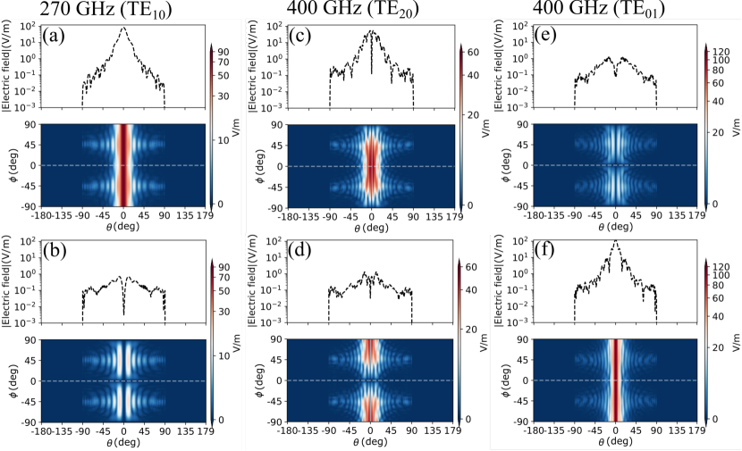
Figure 8: Electro-magnetic far-field simulations of the diagonal-horn antenna at a reference distance of 1 meter from the aperture, performed with the software CST [27]. The images show the absolute value of the electric component of the far-field radiation pattern in the Ludwig-3 coordinate system [34]. The first three propagating modes emitted by the diagonal-horn antenna are shown at reasonably selected frequencies. The white dashed line indicates a cut through the map, shown on top of each figure. (a), (c) and (e) show the co-polarization component $\lvert\boldsymbol{\mathcal{E}}_{\eta}\rvert$ and (b), (d) and (f) show the cross-polarization component $\lvert\boldsymbol{\mathcal{E}}_{\xi}\rvert$, cf. the definition of the $\eta$-$\xi$ aperture coordinate system in Fig. 1(c) of the main text. The far-field intensities of the co- and cross-polarization components for the mode $\mathrm{TE_{10}}$ are approximately interchanged for the mode $\mathrm{TE_{01}}$ and the total absolute electric field in the co- and cross-polarization components for the mode $\mathrm{TE_{20}}$ is approximately the same. This indicates that for the superposition of the three shown propagating modes, the polarization is rotated by $45^{\circ}$ around the wavevector $k_{z}$.

Appendix D Near- and far-field simulations - Part II

This section quantifies the co- and cross-polarization content in the calculated far-field radiation patterns. The final results are summarized in Fig. 9 and show the fundamental mechanism behind the polarization rotation we study in this paper. The data points in Figs. 9(a) and (c) are obtained by integration of far-field patterns like shown in Fig. 8. This obtains the co- and cross-polarization content, $A_{cpol}$ and $A_{crpol}$, of the electric component in the electro-magnetic field, radiated by the diagonal-horn antenna into the free-space. The data points in Figs. 9(b) and (d) are obtained by $\phi,\theta$-integration in the Ludwig-3 coordinate system [34] of the calculated phase-front of the far-field.

Because the aforementioned calculation is important for predicting the polarization dynamics as a function of frequency, the remaining text provides an explanation of the employed formalism.

The field amplitudes in the polarization components are quantified by the integral of the respective absolute value of the sub-THz electric field over the polar coordinates $\theta$ and $\phi$ in the Ludwig-3 coordinate system [35, 34], cf. Fig. 8. We express this formally as follows:

$$A_{cpol}=\int_{S}\lvert{\boldsymbol{\mathcal{E}}_{\eta}}\rvert d\theta d\phi~{},$$ (6a)

$$A_{crpol}=\int_{S}\lvert{\boldsymbol{\mathcal{E}}_{\xi}}\rvert d\theta d\phi~{},$$ (6b)

where $\boldsymbol{\mathcal{E}}_{\eta}$ and $\boldsymbol{\mathcal{E}}_{\xi}$ are the electric far-fields, related to the $\xi$-$\eta$-aperture coordinate system of the diagonal horn, cf. Fig. 1(c), Fig. 3(e)/(iv) and Fig. 5(b), (c) of the main text. This coordinate system is introduced in order to avoid confusion with the $\parallel$- and $\perp$-components of the sub-THz field which are fixed space-wise (and with respect to the silicon-mirror plane of incidence) while the $\xi$-$\eta$ aperture coordinate system is fixed to the frame of the diagonal-horn aperture. For the fundamental $\mathrm{TE}_{10}$-mode, $\boldsymbol{\mathcal{E}}_{\eta}$ is largest and points in direction of the major polarization direction (co-polarization), whereas $\boldsymbol{\mathcal{E}}_{\xi}$ contributes to the much smaller cross-polarization. By rotating the diagonal-horn antenna one aligns either $\boldsymbol{\mathcal{E}}_{\eta}$ or $\boldsymbol{\mathcal{E}}_{\xi}$ with $\boldsymbol{\mathcal{E}}_{\parallel}$ or $\boldsymbol{\mathcal{E}}_{\perp}$.

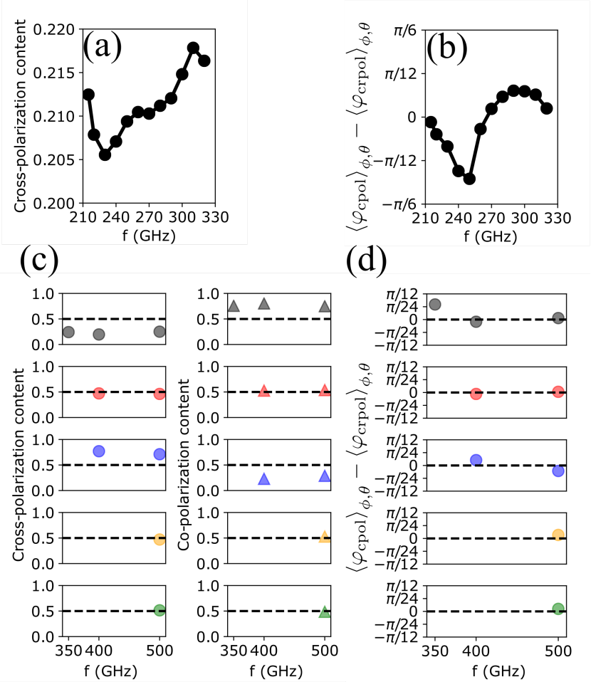
Figure 9: Cross-polarization amplitude content $\mathcal{E}_{crpol}$, (a), and phase difference between the co- and cross-polarization ($\langle\varphi_{\mathrm{cpol}}\rangle_{\phi,\theta}$ - $\langle\varphi_{\mathrm{crpol}}\rangle_{\phi,\theta}$) components, (b), for the $\mathrm{TE}_{10}$ mode. (c) Cross- and co-polarization amplitude content ($\mathcal{E}_{crpol}$ and $\mathcal{E}_{cpol}$) for the $\mathrm{TE}_{10}$ mode and higher order modes for selected frequencies (black $\widehat{=}~{}\mathrm{TE}_{10}$, red $\widehat{=}~{}\mathrm{TE}_{20}$, blue $\widehat{=}~{}\mathrm{TE}_{01}$, orange $\widehat{=}~{}\mathrm{TE}_{11}$ and green $\widehat{=}~{}\mathrm{TM}_{11}$). (d) Phase difference between the co- and cross-polarization components for the modes in (c), showing that the radiated polarization components in each mode are hardly phase shifted with respect to each other. The figure shows results only at selected frequencies, because of the numerically time-consuming simulations. When the first three modes (black, red and blue) propagate for frequencies larger than 400 GHz, a nearly balanced amount of co- and cross-polarization amplitude components are indicative of a polarization rotation by $45^{\circ}$. The other two higher order modes, orange and green, contribute with equal parts to the co- and cross-polarization and, hence, further stabilize the polarization rotation by $45^{\circ}$.

The integration area spanned by the polar coordinates is $S$ on which the far-fields in Fig. 9 are represented. The co- and cross-polarization content in the emitted sub-THz field is then determined by evaluating the expressions:

$$\mathcal{E}_{cpol}=\frac{A_{cpol}}{A_{cpol}+A_{crpol}}~{},$$ (7a)

$$\mathcal{E}_{crpol}=\frac{A_{crpol}}{A_{cpol}+A_{crpol}}~{},$$ (7b)

which are proportional to the field amplitudes in the E- and H-plane, cf. Fig. 3(e)/(iv) of the main text. The right-hand side of the equations are represented in Figs. 9(a) and (c) for the different modes. Equations (6a), (6b), (7a) and (7b) hold for a multimode field and quantify the ratio of $\boldsymbol{\mathcal{E}}_{\eta}$ and $\boldsymbol{\mathcal{E}}_{\xi}$ in the electro-magnetic field.

Higher-order propagating modes in the waveguide create a multimode (in our case up to five) electro-magnetic field. Interestingly, we have discovered that this field has almost equal field strength in the components $\boldsymbol{\mathcal{E}}_{\eta}$ and $\boldsymbol{\mathcal{E}}_{\xi}$ and that these components are practically in-phase (cf. Fig. 9(d)), when radiated from the diagonal-horn antenna into free space. Furthermore, our multimode simulations find that the phase-delay between the aforementioned electric fields in different modes is practically negligible as well. This means, that the different modes are emitted by the diagonal-horn antenna in a coherent fashion and are practically not time-delayed with respect to each other. This is key for an effective polarization rotation of $45^{\circ}$ to happen and for generating a coherent electric field which is then radiated from the near- into the far-field by the diagonal-horn antenna.

Appendix E Imprinting Non-Classical States

The presented results are of interest for single-photon detection using non-classical states of light, as discussed in the review by Ware et al. [36], which is of a very general nature and not directly tied to a specific frequency. The core idea presented in Ware et al. [36] can be understood by means of Fig. 10(a). Here, the central goal is to obtain the efficiency $\eta_{1}$ of the detector. It quantifies how efficient incoming single photons are recorded by the detector and, on the other hand, how many single photons are lost if the detector has not yet reached its fundamentally possible sensitivity.

A straightforward way is to make use of a nonlinear crystal, providing spontaneous parametric down-conversion (sPDC). As a nonlinearity one uses specific crystals that show a nonlinear polarization field response (’polarization’ in this context means the polarization component of the electric displacement field and not the direction of the electric field studied in our paper) when strongly pumped by a laser. In order to exploit this effect, it is strongly pumped by a laser of frequency $f_{p}$ (green wave), and due to the nonlinear interaction, two photons (red and blue wave) of different frequencies, named signal (s) and idler (i), are generated such that the energy and the momentum are conserved,

$$2f_{p} =f_{s}+f_{i}$$ (8a)

$$\boldsymbol{k}_{p} =\boldsymbol{k}_{s}+\boldsymbol{k}_{i}~{}.$$ (8b)

The signal and idler photons are generated at the same time, they are entangled and their power-correlation shows strong two-mode amplitude squeezing below the classical limit, hence, the name non-classical state. Additionally, the outgoing wave polarization is ordinary or extraordinary with respect to the crystal axis. One key feature of this non-classicality is that the detection of one photon out of a pair heralds the presence of the second one. A second detector acting as a trigger, is used to record photon counts in coincidence with the detector, $N_{coinc}$, via two analog-to-digital converters (ADCs). Additionally, the ADCs measure also the photon counts $N_{2}$ of the trigger alone. Because signal and idler photons are generated at the same time, the remarkable advantage of this characterization technique is that the detector efficiency reads then simply [36],

$$\eta_{1}=\frac{N_{coinc}}{N_{2}}$$ (9)

and is independent of the efficiency of the trigger.

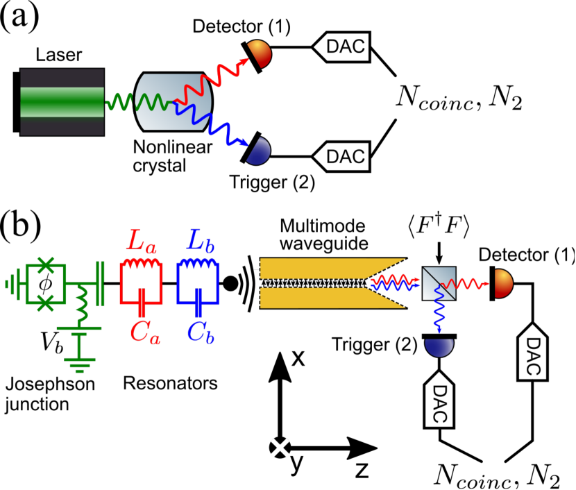
Figure 10: Analogy between photon-pair production during parametric down-conversion in a nonlinear crystal, (a), and due to charge-light coupling in a mesoscopic superconducting two-photon device, (b), like realized in [15, 18, 16, 19] (green, red and blue parts of the figure). In (b), the red and blue photons excite the waveguide (for instance through chip-waveguide coupling [37]) and are radiated in the same or in different polarization states, dependent on their frequencies, into the detector and trigger apertures after scattering off a frequency-selective beamsplitter. The analog-to-digital converters (ADCs) count coincidences $N_{coinc}$ between detector and trigger and photon counts $N_{2}$ of the trigger alone. For detector characterization, the thermal photon population of the environment, $\langle F^{\dagger}F\rangle$, has to be considered.

However, sPDC using a nonlinear crystal is usually an inefficient process and a laser setup is needed. Moreover, due to the momentum conservation, Eq. (8b), the detector and trigger apertures have to be aligned correctly to receive all of the power in order to conduct a proper measurement. Also, the condition Eq. (8b) is frequency dependent such that the emission direction changes when the frequencies are adjusted. Additionally, the outgoing polarized fields usually do not have well defined Gaussian beam properties since the crystal influences the beam shape of the signal and idler fields.

A solution to these difficulties is provided by the two-mode non-classical source demonstrated by Westig et al. [15]. It can be coupled by chip-waveguide coupling [37] to the waveguide in a setup proposed in Fig. 10(b). Since the diagonal-horn antenna at the output of the multimode waveguide provides constant Gaussian beam properties over a large frequency bandwidth, detector and trigger can be kept at constant position. Furthermore, in the example the two-mode non-classical source is based on the dynamical Coulomb blockade of a battery-powered Josephson junction coupled to a tailored electro-magnetic environment, therefore, complex laser setups are not needed.

Together with the progress reported in this paper on the polarization changes of the diagonal-horn antenna as a function of the frequency, a polarization sensitive detector can be characterized using the method of Ware et al. [36]. Specifically, in our proposal a detector and a trigger would be employed which are only sensitive to linearly polarized electro-magnetic fields which is an often encountered technological situation. The task would be to measure the efficiency of such a detector, only sensitive to a linear polarization. The emitted field of the diagonal-horn antenna, excited by the multimode waveguide, provides two options for such a measurement. First, when the signal (red) and the idler (blue) have frequencies such that only the $\mathrm{TE}_{10}$ mode is excited, detector and trigger have to be aligned in such a way to receive the same polarization direction. When the signal frequency remains in the $\mathrm{TE}_{10}$ mode but the idler frequency excites higher order modes, the trigger has to be rotated by $45^{\circ}$ with respect to the detector, cf. Fig. 5(b) and (c). The separation of the different frequencies is achieved by a frequency selective beamsplitter. At the open port of the beamsplitter a thermal photon population is important to quantify, when only a single detector setup would be used for characterization of the detector efficiency. For a correlation setup measuring coincidences like proposed by Fig. 10(b), the thermal photon population does not influence the measurement outcome since it is not correlated at two different frequencies.

References

- nat [2013] Terahertz optics taking off, Nat. Photon. 7, 665 EP (2013), editorial.
- Mittleman [2013] D. M. Mittleman, Frontiers in terahertz sources and plasmonics, Nature Photonics 7, 666 (2013).
- Horiuchi and Zhang [2013] N. Horiuchi and X.-C. Zhang, Bright terahertz sources, Nature Photonics 7, 670 EP (2013).
- Dhillon et al. [2017] S. S. Dhillon, M. S. Vitiello, E. H. Linfield, A. G. Davies, M. C. Hoffmann, J. Booske, C. Paoloni, M. Gensch, P. Weightman, G. P. Williams, et al., The 2017 terahertz science and technology roadmap, Journal of Physics D: Applied Physics 50, 043001 (2017).
- Wallraff et al. [2004] A. Wallraff, D. I. Schuster, A. Blais, L. Frunzio, R.-S. Huang, J. Majer, S. Kumar, S. M. Girvin, and R. J. Schoelkopf, Strong coupling of a single photon to a superconducting qubit using circuit quantum electrodynamics, Nature 431, 162 EP (2004).
- Sanz et al. [2018] M. Sanz, K. G. Fedorov, F. Deppe, and E. Solano, Challenges in open-air microwave quantum communication and sensing, in 2018 IEEE Conference on Antenna Measurements Applications (CAMA) (2018) pp. 1–4.
- Deninger [2013] A. Deninger, 11 - state-of-the-art in terahertz continuous-wave photomixer systems, in Handbook of Terahertz Technology for Imaging, Sensing and Communications, Woodhead Publishing Series in Electronic and Optical Materials, edited by D. Saeedkia (Woodhead Publishing, 2013) pp. 327 – 373.
- Westig et al. [2020] M. Westig, H. Thierschmann, A. Katan, M. Finkel, and T. M. Klapwijk, Analysis of a single-mode waveguide at sub-terahertz frequencies as a communication channel, AIP Advances 10, 015008 (2020), https://doi.org/10.1063/1.5128451 .
- Rolland et al. [2019] C. Rolland, A. Peugeot, S. Dambach, M. Westig, B. Kubala, Y. Mukharsky, C. Altimiras, H. le Sueur, P. Joyez, D. Vion, et al., Antibunched photons emitted by a dc-biased josephson junction, Phys. Rev. Lett. 122, 186804 (2019).
- Gramich et al. [2013] V. Gramich, B. Kubala, S. Rohrer, and J. Ankerhold, From coulomb-blockade to nonlinear quantum dynamics in a superconducting circuit with a resonator, Phys. Rev. Lett. 111, 247002 (2013).
- Dambach et al. [2015] S. Dambach, B. Kubala, V. Gramich, and J. Ankerhold, Time-resolved statistics of nonclassical light in josephson photonics, Phys. Rev. B 92, 054508 (2015).
- Grimm et al. [2019] A. Grimm, F. Blanchet, R. Albert, J. Leppäkangas, S. Jebari, D. Hazra, F. Gustavo, J.-L. Thomassin, E. Dupont-Ferrier, F. Portier, et al., Bright on-demand source of antibunched microwave photons based on inelastic cooper pair tunneling, Phys. Rev. X 9, 021016 (2019).
- Leppäkangas et al. [2015] J. Leppäkangas, M. Fogelström, A. Grimm, M. Hofheinz, M. Marthaler, and G. Johansson, Antibunched photons from inelastic cooper-pair tunneling, Phys. Rev. Lett. 115, 027004 (2015).
- Leppäkangas et al. [2016] J. Leppäkangas, M. Fogelström, M. Marthaler, and G. Johansson, Correlated cooper pair transport and microwave photon emission in the dynamical coulomb blockade, Phys. Rev. B 93, 014506 (2016).
- Westig et al. [2017] M. Westig, B. Kubala, O. Parlavecchio, Y. Mukharsky, C. Altimiras, P. Joyez, D. Vion, P. Roche, D. Esteve, M. Hofheinz, et al., Emission of nonclassical radiation by inelastic cooper pair tunneling, Phys. Rev. Lett. 119, 137001 (2017).
- Leppäkangas et al. [2013] J. Leppäkangas, G. Johansson, M. Marthaler, and M. Fogelström, Nonclassical photon pair production in a voltage-biased josephson junction, Phys. Rev. Lett. 110, 267004 (2013).
- Leppäkangas et al. [2014] J. Leppäkangas, G. Johansson, M. Marthaler, and M. Fogelstr m, Input–output description of microwave radiation in the dynamical coulomb blockade, New Journal of Physics 16, 015015 (2014).
- Armour et al. [2015] A. D. Armour, B. Kubala, and J. Ankerhold, Josephson photonics with a two-mode superconducting circuit, Phys. Rev. B 91, 184508 (2015).
- Trif and Simon [2015] M. Trif and P. Simon, Photon cross-correlations emitted by a josephson junction in two microwave cavities, Phys. Rev. B 92, 014503 (2015).
- Zijlstra et al. [2007] T. Zijlstra, C. F. J. Lodewijk, N. Vercruyssen, F. D. Tichelaar, D. N. Loudkov, and T. M. Klapwijk, Epitaxial aluminum nitride tunnel barriers grown by nitridation with a plasma source, Applied Physics Letters 91, 233102 (2007), https://doi.org/10.1063/1.2819532 .
- Kawamura et al. [1999] J. Kawamura, J. Chen, D. Miller, J. Kooi, J. Zmuidzinas, B. Bumble, H. G. LeDuc, and J. A. Stern, Low-noise submillimeter-wave nbtin superconducting tunnel junction mixers, Applied Physics Letters 75, 4013 (1999), https://doi.org/10.1063/1.125522 .
- Nakamura et al. [2011] Y. Nakamura, H. Terai, K. Inomata, T. Yamamoto, W. Qiu, and Z. Wang, Superconducting qubits consisting of epitaxially grown nbn/aln/nbn josephson junctions, Applied Physics Letters 99, 212502 (2011), https://doi.org/10.1063/1.3663539 .
- Anferov et al. [2020] A. Anferov, A. Suleymanzade, A. Oriani, J. Simon, and D. I. Schuster, Millimeter-wave four-wave mixing via kinetic inductance for quantum devices, Phys. Rev. Applied 13, 024056 (2020).
- Faist et al. [1994] J. Faist, F. Capasso, D. L. Sivco, C. Sirtori, A. L. Hutchinson, and A. Y. Cho, Quantum cascade laser, Science 264, 553 (1994), http://science.sciencemag.org/content/264/5158/553.full.pdf .
- Friedli et al. [2013] P. Friedli, H. Sigg, B. Hinkov, A. Hugi, S. Riedi, M. Beck, and J. Faist, Four-wave mixing in a quantum cascade laser amplifier, Applied Physics Letters 102, 222104 (2013), https://doi.org/10.1063/1.4807662 .
- Justen et al. [2017] M. Justen, K. Otani, D. Turinkov , F. Castellano, M. Beck, U. U. Graf, D. B chel, M. Schultz, and J. Faist, Waveguide Embedding of a Double-Metal 1.9-THz Quantum Cascade Laser: Design, Manufacturing, and Results, IEEE Trans. Terahertz Sci. Technol. 7, 609 (2017).
- [27] CST - Computer Simulation Technology, URL = https://www.cst.com.
- de Graauw, Th. et al. [2010] de Graauw, Th., Helmich, F. P., Phillips, T. G., Stutzki, J., Caux, E., Whyborn, N. D., Dieleman, P., Roelfsema, P. R., Aarts, H., Assendorp, R., et al., The herschel-heterodyne instrument for the far-infrared (hifi)*, A&A 518, L6 (2010).
- [29] We use commercially available GaAs photomixers and the TeraScan 780 system from TOPTICA Photonics AG, Lochhamer Schlag 19, 82166 Gräfelfing/Germany. The source has the specification EK-000831 and the detector has the specification EK-000832. Further specifications are accessible in their online documentation, URL = https://www.toptica.com.
- Born and Wolf [1985] M. Born and E. Wolf, Principles of Optics, sixth (corrected) ed. (Pergamon Press, Headington Hill Hall, Oxford OX3 0BW, England, 1985).
- Roggenbuck et al. [2010] A. Roggenbuck, H. Schmitz, A. Deninger, I. C. Mayorga, J. Hemberger, R. Güsten, and M. Grüninger, Coherent broadband continuous-wave terahertz spectroscopy on solid-state samples, New Journal of Physics 12, 043017 (2010).
- [32] URL = http://www.tydexoptics.com.
- Vogt and Leonhardt [2017] D. W. Vogt and R. Leonhardt, High resolution terahertz spectroscopy of a whispering gallery mode bubble resonator using hilbert analysis, Opt. Express 25, 16860 (2017).
- Ludwig [1973] A. C. Ludwig, The definition of cross polarization, IEEE Trans. Antennas Propagat. 21, 116 (1973).
- Silver and James [1949] S. Silver and H. M. James, eds., Microwave antenna theory and design (McGraw-Hill Book Company, Inc., The Maple Press Company, York, PA, United States of America, 1949) Page 563 explains the experimental method of measuring the co- and cross-polarizations. We employ this method in our electromagnetic-field simulation, shown in Fig. 9.
- Ware and Migdall [2004] M. Ware and A. Migdall, Single-photon detector characterization using correlated photons: The march from feasibility to metrology, Journal of Modern Optics 51, 1549 (2004), https://doi.org/10.1080/09500340408235292 .
- Westig et al. [2011] M. P. Westig, K. Jacobs, J. Stutzki, M. Schultz, M. Justen, and C. E. Honingh, Balanced superconductor–insulator–superconductor mixer on a 9 m silicon membrane, Superconductor Science and Technology 24, 085012 (2011).