Dry Active Matter exhibits a self-organized “Cross Sea” Phase
Abstract
The Vicsek model of self-propelled particles is known in three different phases: a polar ordered homogeneous phase also called Toner-Tu phase, a phase of polar ordered regularly arranged high density bands (waves) with surrounding low density regions without polar order and a homogeneous phase without polar order. It has been questioned whether the band phase should be divided into two parts Chaté (2020): one with periodically arranged and one with strongly interacting but not ordered bands. We answer this question by showing that the standard Vicsek model has a fourth phase for large system sizes: a polar ordered cross sea phase. Close to the transition towards this phase becomes unstable and looks like strongly interacting bands. We demonstrate that the cross sea phase is not just a superposition of two waves, but it is an independent complex pattern. Furthermore we show that there is a non-zero mass flow through the structure of the cross sea pattern within its co-moving frame.
pacs:
05.65+b, 45.70.Qj, 64.60.De, 64.60.EjActive matter is characterized by the transformation of free energy into directed motion. The energy is supplied e.g. by chemicals (or food), external fields or radiation. On the other hand, active particles dissipate energy into their environment such that there is an interplay between energy supply and dissipation. Such processes are clearly far from thermodynamic equilibrium.
Active entities appear from micro length scales or even below e.g. for bacteria, Janus particles or molecular motors up to macroscopic sizes such as for birds, fish, mammals or robots. They might be living organism or artificially manufactured non-living objects. Several reviews give an overview of the field Chaté (2020); Vicsek and Zafeiris (2012); Romanczuk et al. (2012); Ramaswamy (2010); Toner et al. (2005). Theoretical descriptions involve field- or kinetic theories, see e.g. Toner and Tu (1995, 1998); Bertin et al. (2006, 2009); Toner (2012); Ihle (2011, 2016); Nikoubashman and Ihle (2019).
Usually, active particles are surrounded by a fluid like water or air. In many cases the fluid is important, in particular due to the conservation of momentum. Examples are swimming bacteria or artificial microswimmers that are subject to intense research over the last decades, see e.g. Soni et al. (2003); Peruani et al. (2012); Sokolov and Aranson (2012); Dunkel et al. (2013); Gachelin et al. (2014); Karani et al. (2019).
However, there is also a large class of active systems where the fluid can be neglected, e.g. particles moving close to a surface which can transfer arbitrary amounts of momentum to the surrounding, and thus, momentum conservation is effectively not an issue. Such systems with negligible fluid are called dry Chaté (2020) and can be modeled by stochastic equations including positive and negative (activity) dissipation Romanczuk et al. (2012). An important limiting case of strong activation and dissipation leads to a constant particle speed, an ingredient that is often directly incorporated in simplified models. One of such models was introduced 25 years ago by Vicsek et. al. Vicsek et al. (1995) and is one of the simplest and most studied models of active matter until today. In the two-dimensional Vicsek model one considers particles that move with constant speed in individual directions given by angles . Those directions interact at discrete instances of time and remain constant between those collisions. The interactions are given by the following rule
| (1) |
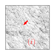
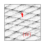
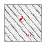
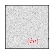
where the set contains the indexes of all particles that satisfy for some interaction radius . The function returns the angle that describes the direction of the two dimensional vector . The are independent random variables drawn uniformly from the interval . That is, after a discrete time interval all particles reorientate due to interactions. They take the average direction of all particles that are within distance , disturbed by random noise of strength . The model exhibits a transition towards collective motion for small noise (or large density) that was first believed to be continuous Vicsek et al. (1995). This shows the non-equilibrium nature of active matter, since in equilibrium such a transition would be strictly forbidden for short-range interactions in two dimensions Mermin and Wagner (1966); Hohenberg (1967). It was found later, that for large enough systems the transition is actually discontinuous and goes along with the formation of high density bands that arrange regularly into waves Grégoire and Chaté (2004); Chaté et al. (2008); Ihle (2013). For even smaller noise strength (or higher density) there is another transition towards a homogeneous polar ordered phase that is also called Toner-Tu phase Chaté et al. (2008); Solon et al. (2015a). The behavior of the model has been described in analogy to a liquid-gas transition Solon et al. (2015a, b). The disordered phase at high noise intensities is considered as a gas, see Fig. 1 for a snapshot of this phase. The phase of polar ordered bands is considered as coexistence of a polar ordered liquid (the bands) and a disordered gas (the particles between the bands with almost no polar order), see Fig. 1 and the Toner-Tu phase is considered as pure polar ordered liquid, see Fig. 1 . It was observed in phase but close to phase that the bands do not achieve a smectic arrangement but they interact strongly and do not order, see Fig. 2b of Ref. Chaté (2020). It was explicitly formulated as a pending issue in Chaté (2020) whether this system states should be considered separately from phase .
In this Letter, we answer this question demonstrating that the aforementioned parameter region represents another fourth phase of the Vicsek model, that has not been reported before to the best of the authors knowledge. In Fig. 1 we show a snapshot of this fourth phase which looks like a cross sea. This is a phenomenon sometimes observed in the oceans when two wave systems like a swell (waves that are no longer under wind influence) and a wind sea (waves generated by wind) are combined, see e.g. Onorato et al. (2010). It is considered to be particularly dangerous for ships, see e.g. Toffoli et al. (2005). Here however, this cross sea pattern is self-organized, since there is no external driving. Furthermore, we demonstrate below that the cross sea pattern of the Vicsek model is not just a superposition of two planar waves. We would also not expect this since nonlinear terms are important in the description of the Vicsek model. In fact, we find that the particle density at the crossing points of the pattern is much higher than the sum of two bands. Thus, particles accumulate at the crossing points of the pattern. Interestingly, similar effects seem to be present also in the cross sea in oceans, see Onorato et al. (2010) and references therein.
We performed simulations for particles in a quadratic domain of size with periodic boundary conditions. Other system parameters are and the noise strength was varied from to in steps of simulating ten realizations for each noise strength. We made snapshots after thermalization time steps 11footnotemark: 1. For the smallest noise strengths we observe more or less homogeneous states. Starting from about structures are formed and for the first cross sea state arises. For all observed realizations are clearly in a cross sea state. Starting from some of the realizations are clearly cross sea and some others are clearly bands, whereas for there are only band state realizations. Eventually, for all realizations are disordered, see supplemental material at pages 6-31. Hence, we observe three transitions between four different phases. The observed mesh sizes and crossing angles of the cross sea pattern vary with parameters but also for different realizations of the same parameter set. Possibly, they are affected by boundary conditions and the orientation of the average direction of motion with respect to the boundary might be important (for system sizes studied here). To answer this question, further studies with significantly more data and a sophisticated image analysis are required.
A system configuration similar to the cross sea state has been shown very recently in Fig. 2b of Chaté (2020). There, it was described as strongly interacting bands that do not order. In view of the results presented here, we can identify this state as very close to the transition between phases and . It looks very similar to the states we find for , see supplemental material.
To study the transitions in greater detail, we investigate a correlation order parameter that was recently introduced in Kürsten et al. (2019) and suggested to be used in the study of structural phase transitions, in particular out of equilibrium. It is a local integral over the two particle correlation function formally given by
| (2) |
where for one- and two-particle probability density functions and , is the Heaviside function. For isotropic systems, the parameter can be expressed in terms of the usual pair correlation function as
| (3) | ||||
Usually, this correlation parameter changes strongly when drastic spatial rearrangements occur. Thus, it is appropriate to study the phase transition that we observe here. Furthermore, it can be sampled efficiently, see Kürsten et al. (2019).
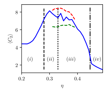
In Fig. 2 we show the average of the order parameter in dependence on the noise strength. It increases drastically at the transition from phase to phase , then it decreases from phase to phase and decreases much more at the transition from phase to phase . In the average over all realizations (solid blue line) we cannot detect the transition between phases and that clearly, since for a relatively large noise range, we find realizations in both states, as discussed above. However, if we measure the order parameter for realizations that show bands or cross sea states separately, we find significant differences in , see dashed red and green lines in Fig. 2. The clear separation of the two dashed lines shows the discontinuous nature of the transition, which is also expected due to the different topological properties of the patterns.
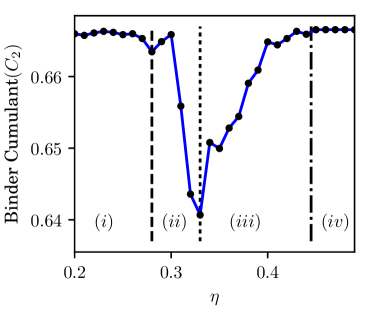
In order to justify whether the cross sea state is really a different phase, we measure the Binder cumulant of the order parameter. In Fig. 3 we see that there are two peaks separating phases and , and and , respectively. In principle, we expect a third peak indicating the transition from phases to . However, it has been shown in Kürsten et al. (2019) that this peak is extremely sharp for large system sizes and thus not covered by the resolution of noise strength used here. As this transition is not the major topic of this Letter, we just roughly estimated its position from looking at the snapshots and plotted it as the dash-dotted line in Fig. 3. The other transition noise strengths obtained from the peaks in the Binder cumulant, and , agree well with the picture we got looking at the snapshots. Remarkably, the peak between phases and is very broad. This can be easily understood, since we already observed that we find some realizations in both states over quite a large noise range. Nevertheless, the peak clearly indicates a phase transition. We expect that the peak is narrowed significantly for much larger systems.
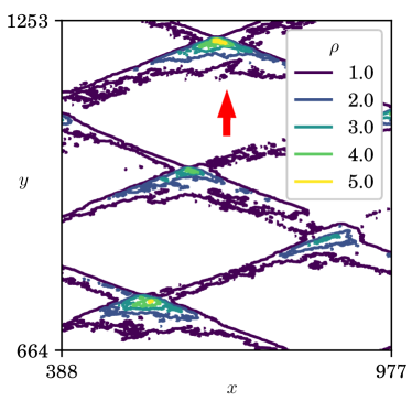
Looking on Fig. 1 we might suppose that the cross sea state is just a superposition of two planar waves as they occur in phase . To verify this hypothesis we measure the particle density averaged in the co-moving frame 222To obtain the pattern co-moving frame we calculated at each time step a histogram of all particles positions before streaming. We then shifted the particle positions after streaming along the axis given by the mean velocity of all particles (among distances not greater than the particle speed ) and also made a histogram of the shifted after-streaming particle positions. We looked for the correlation between the histograms before streaming and after streaming with shift. The shift leading to the maximal correlation was then applied to all particles. of the cross sea pattern. One example is displayed in Fig. 4. We observe that the density at the crossing points of the pattern is much larger than the sum of the densities of two fronts. Hence, we conclude that the cross sea phase represents a standalone complex pattern and not just the sum of two waves.
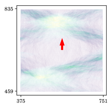
We also investigated the momentum density within the co-moving reference frame of the pattern. We observe a non-zero particle flow along the band structures of the pattern in the direction opposite to the movement of the pattern in the lab frame, see Fig. 5. The appearance of this mass flow is not too surprising since the pattern obeys no symmetry that would forbid such a flow. Furthermore, in this non-equilibrium model we do not expect detailed balance to be present.
In summary, in this numerical study, we have shown that the two-dimensional standard Vicsek model forms complex self-organized cross sea patterns for very large system sizes and in certain parameter regimes. We measured the density profile of the pattern and found that is not just a superposition of two waves but an independent structure. We observe an interesting mass transport in the opposite direction compared to the pattern propagation. Furthermore, measuring the Binder cumulant of a correlation order parameter, we have shown that the cross sea pattern represents a fourth phase of the Vicsek model. There are two transitions from the cross sea phase: for lower noise intensity the system enters the Toner-Tu phase and for higher noise intensity it enters the phase of high density waves. We thus answer a recently formulated question Chaté (2020). On the other hand, an theoretical understanding of this novel phase is still missing. Natural candidates for mathematical descriptions are field- or kinetic theories. Both approaches seem to be challenging, since a full two-dimensional treatment is likely to be necessary in contrast to the band phase. The appearance of the cross sea phase is likely to be relevant also for other models, similar to the Vicsek model. However, further studies are required. Another pending question is whether an analogous phase exists in the three-dimensional Vicsek model. A remarkable result from the general view on active matter is that apparently single species active systems can form complex patterns similar to those known from reaction-diffusion systems.
Acknowledgements.
The authors gratefully acknowledges the GWK support for funding this project by providing computing time through the Center for Information Services and HPC (ZIH) at TU Dresden on the HRSK-II. The authors gratefully acknowledges the Universitätsrechenzentrum Greifswald for providing computing time.References
- Chaté (2020) H. Chaté, Annu. Rev. Condens. Matter Phys. 11, 189 (2020).
- Vicsek and Zafeiris (2012) T. Vicsek and A. Zafeiris, Phys. Rep. 517, 71 (2012).
- Romanczuk et al. (2012) P. Romanczuk, M. Bär, W. Ebeling, B. Lindner, and L. Schimansky-Geier, Eur. Phys. J. - Spec. Top. 202, 1 (2012).
- Ramaswamy (2010) S. Ramaswamy, Annu. Rev. Condens. Matter Phys. 1, 323 (2010).
- Toner et al. (2005) J. Toner, Y. Tu, and S. Ramaswamy, Ann. Phys. 318, 170 (2005).
- Toner and Tu (1995) J. Toner and Y. Tu, Phys. Rev. Lett. 75, 4326 (1995).
- Toner and Tu (1998) J. Toner and Y. Tu, Phys. Rev. E 58, 4828 (1998).
- Bertin et al. (2006) E. Bertin, M. Droz, and G. Grégoire, Phys. Rev. E 74, 022101 (2006).
- Bertin et al. (2009) E. Bertin, M. Droz, and G. Grégoire, J. Phys. A: Math. Theor. 42, 445001 (2009).
- Toner (2012) J. Toner, Phys. Rev. E 86, 031918 (2012).
- Ihle (2011) T. Ihle, Phys. Rev. E 83, 030901 (2011).
- Ihle (2016) T. Ihle, J. Stat. Mech. - Theory E. 2016, 083205 (2016).
- Nikoubashman and Ihle (2019) A. Nikoubashman and T. Ihle, Phys. Rev. E 100, 042603 (2019).
- Soni et al. (2003) G. Soni, B. J. Ali, Y. Hatwalne, and G. Shivashankar, Biophys. J. 84, 2634 (2003).
- Peruani et al. (2012) F. Peruani, J. Starruß, V. Jakovljevic, L. Søgaard-Andersen, A. Deutsch, and M. Bär, Phys. Rev. Lett. 108, 098102 (2012).
- Sokolov and Aranson (2012) A. Sokolov and I. S. Aranson, Phys. Rev. Lett. 109, 248109 (2012).
- Dunkel et al. (2013) J. Dunkel, S. Heidenreich, K. Drescher, H. H. Wensink, M. Bär, and R. E. Goldstein, Phys. Rev. Lett. 110, 228102 (2013).
- Gachelin et al. (2014) J. Gachelin, A. Rousselet, A. Lindner, and E. Clement, New J. Phys. 16, 025003 (2014).
- Karani et al. (2019) H. Karani, G. E. Pradillo, and P. M. Vlahovska, Phys. Rev. Lett. 123, 208002 (2019).
- Vicsek et al. (1995) T. Vicsek, A. Czirók, E. Ben-Jacob, I. Cohen, and O. Shochet, Phys. Rev. Lett. 75, 1226 (1995).
- Mermin and Wagner (1966) N. D. Mermin and H. Wagner, Phys. Rev. Lett. 17, 1133 (1966).
- Hohenberg (1967) P. C. Hohenberg, Phys. Rev. 158, 383 (1967).
- Grégoire and Chaté (2004) G. Grégoire and H. Chaté, Phys. Rev. Lett. 92, 025702 (2004).
- Chaté et al. (2008) H. Chaté, F. Ginelli, G. Grégoire, and F. Raynaud, Phys. Rev. E 77, 046113 (2008).
- Ihle (2013) T. Ihle, Phys. Rev. E 88, 040303 (2013).
- Solon et al. (2015a) A. P. Solon, H. Chaté, and J. Tailleur, Phys. Rev. Lett. 114, 068101 (2015a).
- Solon et al. (2015b) A. P. Solon, J.-B. Caussin, D. Bartolo, H. Chaté, and J. Tailleur, Phys. Rev. E 92, 062111 (2015b).
- Onorato et al. (2010) M. Onorato, D. Proment, and A. Toffoli, Eur. Phys. J. - Spec. Top. 185, 45 (2010).
- Toffoli et al. (2005) A. Toffoli, J. Lefevre, E. Bitner-Gregersen, and J. Monbaliu, Appl. Ocean Res. 27, 281 (2005).
- Note (1) For the smallest noise strength in the disordered phase, , we still used , for lager noise stengths, we used a shorter time of since thermalization is much faster in the disordered phase.
- Kürsten et al. (2019) R. Kürsten, S. Stroteich, M. Zumaya-Hérnandez, and T. Ihle, (2019), arXiv:1910.04244 [cond-mat.soft] .
- Note (2) To obtain the pattern co-moving frame we calculated at each time step a histogram of all particles positions before streaming. We then shifted the particle positions after streaming along the axis given by the mean velocity of all particles (among distances not greater than the particle speed ) and also made a histogram of the shifted after-streaming particle positions. We looked for the correlation between the histograms before streaming and after streaming with shift. The shift leading to the maximal correlation was then applied to all particles.
Appendix A Supplemental material: Snapshots of ten realizations, all started from random initial conditions, parameters as in the letter.
.
![[Uncaptioned image]](/html/2002.03198/assets/r1eta0_20.jpg)
![[Uncaptioned image]](/html/2002.03198/assets/r2eta0_20.jpg)
![[Uncaptioned image]](/html/2002.03198/assets/r3eta0_20.jpg)
![[Uncaptioned image]](/html/2002.03198/assets/r4eta0_20.jpg)
![[Uncaptioned image]](/html/2002.03198/assets/r5eta0_20.jpg)
![[Uncaptioned image]](/html/2002.03198/assets/r6eta0_20.jpg)
![[Uncaptioned image]](/html/2002.03198/assets/r7eta0_20.jpg)
![[Uncaptioned image]](/html/2002.03198/assets/r8eta0_20.jpg)
![[Uncaptioned image]](/html/2002.03198/assets/r9eta0_20.jpg)
![[Uncaptioned image]](/html/2002.03198/assets/r10eta0_20.jpg)
.
![[Uncaptioned image]](/html/2002.03198/assets/r1eta0_21.jpg)
![[Uncaptioned image]](/html/2002.03198/assets/r2eta0_21.jpg)
![[Uncaptioned image]](/html/2002.03198/assets/r3eta0_21.jpg)
![[Uncaptioned image]](/html/2002.03198/assets/r4eta0_21.jpg)
![[Uncaptioned image]](/html/2002.03198/assets/r5eta0_21.jpg)
![[Uncaptioned image]](/html/2002.03198/assets/r6eta0_21.jpg)
![[Uncaptioned image]](/html/2002.03198/assets/r7eta0_21.jpg)
![[Uncaptioned image]](/html/2002.03198/assets/r8eta0_21.jpg)
![[Uncaptioned image]](/html/2002.03198/assets/r9eta0_21.jpg)
![[Uncaptioned image]](/html/2002.03198/assets/r10eta0_21.jpg)
.
![[Uncaptioned image]](/html/2002.03198/assets/r1eta0_22.jpg)
![[Uncaptioned image]](/html/2002.03198/assets/r2eta0_22.jpg)
![[Uncaptioned image]](/html/2002.03198/assets/r3eta0_22.jpg)
![[Uncaptioned image]](/html/2002.03198/assets/r4eta0_22.jpg)
![[Uncaptioned image]](/html/2002.03198/assets/r5eta0_22.jpg)
![[Uncaptioned image]](/html/2002.03198/assets/r6eta0_22.jpg)
![[Uncaptioned image]](/html/2002.03198/assets/r7eta0_22.jpg)
![[Uncaptioned image]](/html/2002.03198/assets/r8eta0_22.jpg)
![[Uncaptioned image]](/html/2002.03198/assets/r9eta0_22.jpg)
![[Uncaptioned image]](/html/2002.03198/assets/r10eta0_22.jpg)
.
![[Uncaptioned image]](/html/2002.03198/assets/r1eta0_23.jpg)
![[Uncaptioned image]](/html/2002.03198/assets/r2eta0_23.jpg)
![[Uncaptioned image]](/html/2002.03198/assets/r3eta0_23.jpg)
![[Uncaptioned image]](/html/2002.03198/assets/r4eta0_23.jpg)
![[Uncaptioned image]](/html/2002.03198/assets/r5eta0_23.jpg)
![[Uncaptioned image]](/html/2002.03198/assets/r6eta0_23.jpg)
![[Uncaptioned image]](/html/2002.03198/assets/r7eta0_23.jpg)
![[Uncaptioned image]](/html/2002.03198/assets/r8eta0_23.jpg)
![[Uncaptioned image]](/html/2002.03198/assets/r9eta0_23.jpg)
![[Uncaptioned image]](/html/2002.03198/assets/r10eta0_23.jpg)
.
![[Uncaptioned image]](/html/2002.03198/assets/r1eta0_24.jpg)
![[Uncaptioned image]](/html/2002.03198/assets/r2eta0_24.jpg)
![[Uncaptioned image]](/html/2002.03198/assets/r3eta0_24.jpg)
![[Uncaptioned image]](/html/2002.03198/assets/r4eta0_24.jpg)
![[Uncaptioned image]](/html/2002.03198/assets/r5eta0_24.jpg)
![[Uncaptioned image]](/html/2002.03198/assets/r6eta0_24.jpg)
![[Uncaptioned image]](/html/2002.03198/assets/r7eta0_24.jpg)
![[Uncaptioned image]](/html/2002.03198/assets/r8eta0_24.jpg)
![[Uncaptioned image]](/html/2002.03198/assets/r9eta0_24.jpg)
![[Uncaptioned image]](/html/2002.03198/assets/r10eta0_24.jpg)
.
![[Uncaptioned image]](/html/2002.03198/assets/r1eta0_25.jpg)
![[Uncaptioned image]](/html/2002.03198/assets/r2eta0_25.jpg)
![[Uncaptioned image]](/html/2002.03198/assets/r3eta0_25.jpg)
![[Uncaptioned image]](/html/2002.03198/assets/r4eta0_25.jpg)
![[Uncaptioned image]](/html/2002.03198/assets/r5eta0_25.jpg)
![[Uncaptioned image]](/html/2002.03198/assets/r6eta0_25.jpg)
![[Uncaptioned image]](/html/2002.03198/assets/r7eta0_25.jpg)
![[Uncaptioned image]](/html/2002.03198/assets/r8eta0_25.jpg)
![[Uncaptioned image]](/html/2002.03198/assets/r9eta0_25.jpg)
![[Uncaptioned image]](/html/2002.03198/assets/r10eta0_25.jpg)
.
![[Uncaptioned image]](/html/2002.03198/assets/r1eta0_26.jpg)
![[Uncaptioned image]](/html/2002.03198/assets/r2eta0_26.jpg)
![[Uncaptioned image]](/html/2002.03198/assets/r3eta0_26.jpg)
![[Uncaptioned image]](/html/2002.03198/assets/r4eta0_26.jpg)
![[Uncaptioned image]](/html/2002.03198/assets/r5eta0_26.jpg)
![[Uncaptioned image]](/html/2002.03198/assets/r6eta0_26.jpg)
![[Uncaptioned image]](/html/2002.03198/assets/r7eta0_26.jpg)
![[Uncaptioned image]](/html/2002.03198/assets/r8eta0_26.jpg)
![[Uncaptioned image]](/html/2002.03198/assets/r9eta0_26.jpg)
![[Uncaptioned image]](/html/2002.03198/assets/r10eta0_26.jpg)
.
![[Uncaptioned image]](/html/2002.03198/assets/r1eta0_27.jpg)
![[Uncaptioned image]](/html/2002.03198/assets/r2eta0_27.jpg)
![[Uncaptioned image]](/html/2002.03198/assets/r3eta0_27.jpg)
![[Uncaptioned image]](/html/2002.03198/assets/r4eta0_27.jpg)
![[Uncaptioned image]](/html/2002.03198/assets/r5eta0_27.jpg)
![[Uncaptioned image]](/html/2002.03198/assets/r6eta0_27.jpg)
![[Uncaptioned image]](/html/2002.03198/assets/r7eta0_27.jpg)
![[Uncaptioned image]](/html/2002.03198/assets/r8eta0_27.jpg)
![[Uncaptioned image]](/html/2002.03198/assets/r9eta0_27.jpg)
![[Uncaptioned image]](/html/2002.03198/assets/r10eta0_27.jpg)
.
![[Uncaptioned image]](/html/2002.03198/assets/r1eta0_28.jpg)
![[Uncaptioned image]](/html/2002.03198/assets/r2eta0_28.jpg)
![[Uncaptioned image]](/html/2002.03198/assets/r3eta0_28.jpg)
![[Uncaptioned image]](/html/2002.03198/assets/r4eta0_28.jpg)
![[Uncaptioned image]](/html/2002.03198/assets/r5eta0_28.jpg)
![[Uncaptioned image]](/html/2002.03198/assets/r6eta0_28.jpg)
![[Uncaptioned image]](/html/2002.03198/assets/r7eta0_28.jpg)
![[Uncaptioned image]](/html/2002.03198/assets/r8eta0_28.jpg)
![[Uncaptioned image]](/html/2002.03198/assets/r9eta0_28.jpg)
![[Uncaptioned image]](/html/2002.03198/assets/r10eta0_28.jpg)
.
![[Uncaptioned image]](/html/2002.03198/assets/r1eta0_29.jpg)
![[Uncaptioned image]](/html/2002.03198/assets/r2eta0_29.jpg)
![[Uncaptioned image]](/html/2002.03198/assets/r3eta0_29.jpg)
![[Uncaptioned image]](/html/2002.03198/assets/r4eta0_29.jpg)
![[Uncaptioned image]](/html/2002.03198/assets/r5eta0_29.jpg)
![[Uncaptioned image]](/html/2002.03198/assets/r6eta0_29.jpg)
![[Uncaptioned image]](/html/2002.03198/assets/r7eta0_29.jpg)
![[Uncaptioned image]](/html/2002.03198/assets/r8eta0_29.jpg)
![[Uncaptioned image]](/html/2002.03198/assets/r9eta0_29.jpg)
![[Uncaptioned image]](/html/2002.03198/assets/r10eta0_29.jpg)
.
![[Uncaptioned image]](/html/2002.03198/assets/r1eta0_30.jpg)
![[Uncaptioned image]](/html/2002.03198/assets/r2eta0_30.jpg)
![[Uncaptioned image]](/html/2002.03198/assets/r3eta0_30.jpg)
![[Uncaptioned image]](/html/2002.03198/assets/r4eta0_30.jpg)
![[Uncaptioned image]](/html/2002.03198/assets/r5eta0_30.jpg)
![[Uncaptioned image]](/html/2002.03198/assets/r6eta0_30.jpg)
![[Uncaptioned image]](/html/2002.03198/assets/r7eta0_30.jpg)
![[Uncaptioned image]](/html/2002.03198/assets/r8eta0_30.jpg)
![[Uncaptioned image]](/html/2002.03198/assets/r9eta0_30.jpg)
![[Uncaptioned image]](/html/2002.03198/assets/r10eta0_30.jpg)
.
![[Uncaptioned image]](/html/2002.03198/assets/r1eta0_31.jpg)
![[Uncaptioned image]](/html/2002.03198/assets/r2eta0_31.jpg)
![[Uncaptioned image]](/html/2002.03198/assets/r3eta0_31.jpg)
![[Uncaptioned image]](/html/2002.03198/assets/r4eta0_31.jpg)
![[Uncaptioned image]](/html/2002.03198/assets/r5eta0_31.jpg)
![[Uncaptioned image]](/html/2002.03198/assets/r6eta0_31.jpg)
![[Uncaptioned image]](/html/2002.03198/assets/r7eta0_31.jpg)
![[Uncaptioned image]](/html/2002.03198/assets/r8eta0_31.jpg)
![[Uncaptioned image]](/html/2002.03198/assets/r9eta0_31.jpg)
![[Uncaptioned image]](/html/2002.03198/assets/r10eta0_31.jpg)
.
![[Uncaptioned image]](/html/2002.03198/assets/r1eta0_32.jpg)
![[Uncaptioned image]](/html/2002.03198/assets/r2eta0_32.jpg)
![[Uncaptioned image]](/html/2002.03198/assets/r3eta0_32.jpg)
![[Uncaptioned image]](/html/2002.03198/assets/r4eta0_32.jpg)
![[Uncaptioned image]](/html/2002.03198/assets/r5eta0_32.jpg)
![[Uncaptioned image]](/html/2002.03198/assets/r6eta0_32.jpg)
![[Uncaptioned image]](/html/2002.03198/assets/r7eta0_32.jpg)
![[Uncaptioned image]](/html/2002.03198/assets/r8eta0_32.jpg)
![[Uncaptioned image]](/html/2002.03198/assets/r9eta0_32.jpg)
![[Uncaptioned image]](/html/2002.03198/assets/r10eta0_32.jpg)
.
![[Uncaptioned image]](/html/2002.03198/assets/r1eta0_33.jpg)
![[Uncaptioned image]](/html/2002.03198/assets/r2eta0_33.jpg)
![[Uncaptioned image]](/html/2002.03198/assets/r3eta0_33.jpg)
![[Uncaptioned image]](/html/2002.03198/assets/r4eta0_33.jpg)
![[Uncaptioned image]](/html/2002.03198/assets/r5eta0_33.jpg)
![[Uncaptioned image]](/html/2002.03198/assets/r6eta0_33.jpg)
![[Uncaptioned image]](/html/2002.03198/assets/r7eta0_33.jpg)
![[Uncaptioned image]](/html/2002.03198/assets/r8eta0_33.jpg)
![[Uncaptioned image]](/html/2002.03198/assets/r9eta0_33.jpg)
![[Uncaptioned image]](/html/2002.03198/assets/r10eta0_33.jpg)
.
![[Uncaptioned image]](/html/2002.03198/assets/r1eta0_34.jpg)
![[Uncaptioned image]](/html/2002.03198/assets/r2eta0_34.jpg)
![[Uncaptioned image]](/html/2002.03198/assets/r3eta0_34.jpg)
![[Uncaptioned image]](/html/2002.03198/assets/r4eta0_34.jpg)
![[Uncaptioned image]](/html/2002.03198/assets/r5eta0_34.jpg)
![[Uncaptioned image]](/html/2002.03198/assets/r6eta0_34.jpg)
![[Uncaptioned image]](/html/2002.03198/assets/r7eta0_34.jpg)
![[Uncaptioned image]](/html/2002.03198/assets/r8eta0_34.jpg)
![[Uncaptioned image]](/html/2002.03198/assets/r9eta0_34.jpg)
![[Uncaptioned image]](/html/2002.03198/assets/r10eta0_34.jpg)
.
![[Uncaptioned image]](/html/2002.03198/assets/r1eta0_35.jpg)
![[Uncaptioned image]](/html/2002.03198/assets/r2eta0_35.jpg)
![[Uncaptioned image]](/html/2002.03198/assets/r3eta0_35.jpg)
![[Uncaptioned image]](/html/2002.03198/assets/r4eta0_35.jpg)
![[Uncaptioned image]](/html/2002.03198/assets/r5eta0_35.jpg)
![[Uncaptioned image]](/html/2002.03198/assets/r6eta0_35.jpg)
![[Uncaptioned image]](/html/2002.03198/assets/r7eta0_35.jpg)
![[Uncaptioned image]](/html/2002.03198/assets/r8eta0_35.jpg)
![[Uncaptioned image]](/html/2002.03198/assets/r9eta0_35.jpg)
![[Uncaptioned image]](/html/2002.03198/assets/r10eta0_35.jpg)
.
![[Uncaptioned image]](/html/2002.03198/assets/r1eta0_36.jpg)
![[Uncaptioned image]](/html/2002.03198/assets/r2eta0_36.jpg)
![[Uncaptioned image]](/html/2002.03198/assets/r3eta0_36.jpg)
![[Uncaptioned image]](/html/2002.03198/assets/r4eta0_36.jpg)
![[Uncaptioned image]](/html/2002.03198/assets/r5eta0_36.jpg)
![[Uncaptioned image]](/html/2002.03198/assets/r6eta0_36.jpg)
![[Uncaptioned image]](/html/2002.03198/assets/r7eta0_36.jpg)
![[Uncaptioned image]](/html/2002.03198/assets/r8eta0_36.jpg)
![[Uncaptioned image]](/html/2002.03198/assets/r9eta0_36.jpg)
![[Uncaptioned image]](/html/2002.03198/assets/r10eta0_36.jpg)
.
![[Uncaptioned image]](/html/2002.03198/assets/r1eta0_37.jpg)
![[Uncaptioned image]](/html/2002.03198/assets/r2eta0_37.jpg)
![[Uncaptioned image]](/html/2002.03198/assets/r3eta0_37.jpg)
![[Uncaptioned image]](/html/2002.03198/assets/r4eta0_37.jpg)
![[Uncaptioned image]](/html/2002.03198/assets/r5eta0_37.jpg)
![[Uncaptioned image]](/html/2002.03198/assets/r6eta0_37.jpg)
![[Uncaptioned image]](/html/2002.03198/assets/r7eta0_37.jpg)
![[Uncaptioned image]](/html/2002.03198/assets/r8eta0_37.jpg)
![[Uncaptioned image]](/html/2002.03198/assets/r9eta0_37.jpg)
![[Uncaptioned image]](/html/2002.03198/assets/r10eta0_37.jpg)
.
![[Uncaptioned image]](/html/2002.03198/assets/r1eta0_38.jpg)
![[Uncaptioned image]](/html/2002.03198/assets/r2eta0_38.jpg)
![[Uncaptioned image]](/html/2002.03198/assets/r3eta0_38.jpg)
![[Uncaptioned image]](/html/2002.03198/assets/r4eta0_38.jpg)
![[Uncaptioned image]](/html/2002.03198/assets/r5eta0_38.jpg)
![[Uncaptioned image]](/html/2002.03198/assets/r6eta0_38.jpg)
![[Uncaptioned image]](/html/2002.03198/assets/r7eta0_38.jpg)
![[Uncaptioned image]](/html/2002.03198/assets/r8eta0_38.jpg)
![[Uncaptioned image]](/html/2002.03198/assets/r9eta0_38.jpg)
![[Uncaptioned image]](/html/2002.03198/assets/r10eta0_38.jpg)
.
![[Uncaptioned image]](/html/2002.03198/assets/r1eta0_39.jpg)
![[Uncaptioned image]](/html/2002.03198/assets/r2eta0_39.jpg)
![[Uncaptioned image]](/html/2002.03198/assets/r3eta0_39.jpg)
![[Uncaptioned image]](/html/2002.03198/assets/r4eta0_39.jpg)
![[Uncaptioned image]](/html/2002.03198/assets/r5eta0_39.jpg)
![[Uncaptioned image]](/html/2002.03198/assets/r6eta0_39.jpg)
![[Uncaptioned image]](/html/2002.03198/assets/r7eta0_39.jpg)
![[Uncaptioned image]](/html/2002.03198/assets/r8eta0_39.jpg)
![[Uncaptioned image]](/html/2002.03198/assets/r9eta0_39.jpg)
![[Uncaptioned image]](/html/2002.03198/assets/r10eta0_39.jpg)
.
![[Uncaptioned image]](/html/2002.03198/assets/r1eta0_40.jpg)
![[Uncaptioned image]](/html/2002.03198/assets/r2eta0_40.jpg)
![[Uncaptioned image]](/html/2002.03198/assets/r3eta0_40.jpg)
![[Uncaptioned image]](/html/2002.03198/assets/r4eta0_40.jpg)
![[Uncaptioned image]](/html/2002.03198/assets/r5eta0_40.jpg)
![[Uncaptioned image]](/html/2002.03198/assets/r6eta0_40.jpg)
![[Uncaptioned image]](/html/2002.03198/assets/r7eta0_40.jpg)
![[Uncaptioned image]](/html/2002.03198/assets/r8eta0_40.jpg)
![[Uncaptioned image]](/html/2002.03198/assets/r9eta0_40.jpg)
![[Uncaptioned image]](/html/2002.03198/assets/r10eta0_40.jpg)
.
![[Uncaptioned image]](/html/2002.03198/assets/r1eta0_41.jpg)
![[Uncaptioned image]](/html/2002.03198/assets/r2eta0_41.jpg)
![[Uncaptioned image]](/html/2002.03198/assets/r3eta0_41.jpg)
![[Uncaptioned image]](/html/2002.03198/assets/r4eta0_41.jpg)
![[Uncaptioned image]](/html/2002.03198/assets/r5eta0_41.jpg)
![[Uncaptioned image]](/html/2002.03198/assets/r6eta0_41.jpg)
![[Uncaptioned image]](/html/2002.03198/assets/r7eta0_41.jpg)
![[Uncaptioned image]](/html/2002.03198/assets/r8eta0_41.jpg)
![[Uncaptioned image]](/html/2002.03198/assets/r9eta0_41.jpg)
![[Uncaptioned image]](/html/2002.03198/assets/r10eta0_41.jpg)
.
![[Uncaptioned image]](/html/2002.03198/assets/r1eta0_42.jpg)
![[Uncaptioned image]](/html/2002.03198/assets/r2eta0_42.jpg)
![[Uncaptioned image]](/html/2002.03198/assets/r3eta0_42.jpg)
![[Uncaptioned image]](/html/2002.03198/assets/r4eta0_42.jpg)
![[Uncaptioned image]](/html/2002.03198/assets/r5eta0_42.jpg)
![[Uncaptioned image]](/html/2002.03198/assets/r6eta0_42.jpg)
![[Uncaptioned image]](/html/2002.03198/assets/r7eta0_42.jpg)
![[Uncaptioned image]](/html/2002.03198/assets/r8eta0_42.jpg)
![[Uncaptioned image]](/html/2002.03198/assets/r9eta0_42.jpg)
![[Uncaptioned image]](/html/2002.03198/assets/r10eta0_42.jpg)
.
![[Uncaptioned image]](/html/2002.03198/assets/r1eta0_43.jpg)
![[Uncaptioned image]](/html/2002.03198/assets/r2eta0_43.jpg)
![[Uncaptioned image]](/html/2002.03198/assets/r3eta0_43.jpg)
![[Uncaptioned image]](/html/2002.03198/assets/r4eta0_43.jpg)
![[Uncaptioned image]](/html/2002.03198/assets/r5eta0_43.jpg)
![[Uncaptioned image]](/html/2002.03198/assets/r6eta0_43.jpg)
![[Uncaptioned image]](/html/2002.03198/assets/r7eta0_43.jpg)
![[Uncaptioned image]](/html/2002.03198/assets/r8eta0_43.jpg)
![[Uncaptioned image]](/html/2002.03198/assets/r9eta0_43.jpg)
![[Uncaptioned image]](/html/2002.03198/assets/r10eta0_43.jpg)
.
![[Uncaptioned image]](/html/2002.03198/assets/r1eta0_44.jpg)
![[Uncaptioned image]](/html/2002.03198/assets/r2eta0_44.jpg)
![[Uncaptioned image]](/html/2002.03198/assets/r3eta0_44.jpg)
![[Uncaptioned image]](/html/2002.03198/assets/r4eta0_44.jpg)
![[Uncaptioned image]](/html/2002.03198/assets/r5eta0_44.jpg)
![[Uncaptioned image]](/html/2002.03198/assets/r6eta0_44.jpg)
![[Uncaptioned image]](/html/2002.03198/assets/r7eta0_44.jpg)
![[Uncaptioned image]](/html/2002.03198/assets/r8eta0_44.jpg)
![[Uncaptioned image]](/html/2002.03198/assets/r9eta0_44.jpg)
![[Uncaptioned image]](/html/2002.03198/assets/r10eta0_44.jpg)
.
![[Uncaptioned image]](/html/2002.03198/assets/r1eta0_45.jpg)
![[Uncaptioned image]](/html/2002.03198/assets/r2eta0_45.jpg)
![[Uncaptioned image]](/html/2002.03198/assets/r3eta0_45.jpg)
![[Uncaptioned image]](/html/2002.03198/assets/r4eta0_45.jpg)
![[Uncaptioned image]](/html/2002.03198/assets/r5eta0_45.jpg)
![[Uncaptioned image]](/html/2002.03198/assets/r6eta0_45.jpg)
![[Uncaptioned image]](/html/2002.03198/assets/r7eta0_45.jpg)
![[Uncaptioned image]](/html/2002.03198/assets/r8eta0_45.jpg)
![[Uncaptioned image]](/html/2002.03198/assets/r9eta0_45.jpg)
![[Uncaptioned image]](/html/2002.03198/assets/r10eta0_45.jpg)
Snapshots for look very similar to those at and are not presented here.