Optimal topological generators of $U(1)$

Abstract.

Sarnak’s golden mean conjecture states that $(m+1)d_{\varphi}(m)\leqslant 1+\frac{2}{\sqrt{5}}$ for all integers $m\geqslant 1$, where $\varphi$ is the golden mean and $d_{\theta}$ is the discrepancy function for $m+1$ multiples of $\theta$ modulo 1. In this paper, we characterize the set $\mathcal{S}$ of values $\theta$ that share this property, as well as the set $\mathcal{T}$ of those with the property for some lower bound $m\geqslant M$. Remarkably, $\mathcal{S}\operatorname{mod}1$ has only 16 elements, whereas $\mathcal{T}$ is the set of $GL_{2}(\mathbb{Z})$-transformations of $\varphi$.

1. Introduction

The unitary group $U(1)$ is compact with an invariant measure, and which may be modeled as acting by rotation on the circle $S^{1}\subset\mathbb{C}$ taken to have length 1. It is well known in this model that $U(1)$ is (monogenically) topologically generated by a rotation by any irrational angle. A natural question here is which of these topological generators is the best. To answer this inquiry, we introduce the following function:

Definition (cf. [1]).

Let $[[m]]=\{0,\dots,m\}$. Define $d_{\theta}(m)$ as

$$\sup\{\left\lvert I\right\rvert:\text{$I\subset\mathbb{R}$ an interval},(I+\mathbb{Z})\cap[[m]]\theta=\varnothing\}.$$

$d_{\theta}(m)$ measures the largest “gap,” modulo 1, of $m+1$ consecutive integer multiples of the real number $\theta$. It is clear that if $\theta$ is rational with the reduced fraction representation $\theta=\frac{a}{b}$, then $d_{\theta}(m)=\frac{1}{b}$ for all $m\geqslant b-1$. Meanwhile, when $\theta$ is irrational it is a topological generator of $U(1)$, so

$$\lim\limits_{m\to\infty}d_{\theta}(m)=0$$

weakly monotonically. For all choices of $\theta$, $(m+1)d_{\theta}(m)\geqslant 1$ since equality is attained precisely when $d_{\theta}(m)=\frac{1}{m+1}$, but by the pigeonhole principle, $d_{\theta}(m)\geqslant\frac{1}{m+1}$. Therefore, $d_{\theta}(m)$ can be thought of as the discrepancy between the first $m+1$ iterates of $\theta$ and an equidistribution, and $(m+1)d_{\theta}(m)$ can be thought of as measuring how quickly $d_{\theta}(m)$ tends to 0 for irrational $\theta$.

Graham and van Lint [1] studied asymptotic behavior of this quantity, using the language of continued fractions. We say that two continued fractions $\theta$ and $\sigma$ are equivalent, written $\theta\asymp\sigma$, if there are positive integers $m$ and $n$ such that $\theta$ and $\sigma$ agree after removing the length-$m$ and length-$n$ prefixes, respectively. The golden ratio is $\varphi=\frac{1+\sqrt{5}}{2}$, and has continued fraction consisting of all 1’s.

Theorem ([1], Theorem 2).

For any irrational $\theta$,

$$\limsup\limits_{m\to\infty}(m+1)d_{\theta}(m)\geqslant 1+\frac{2}{\sqrt{5}}$$

with equality iff $\theta\asymp\varphi$.

Here, we prove a stronger result about these asymptotics:

Theorem 1.

Given $\theta\in\mathbb{R}$, there exists $M\in\mathbb{N}$ for which $m\geqslant M$ implies $(m+1)d_{\theta}(m)<1+\frac{2}{\sqrt{5}}$ if and only if $\theta\asymp\varphi$.

Letting $\mathcal{T}$ be the set of values $\theta$ for which the condition on $d_{\theta}(m)$ in Theorem 1 holds, we will see, as is well known, that $\mathcal{T}$ is the set of linear fractional transformations by $GL_{2}(\mathbb{Z})$ of $\varphi$, a dense countable subset of $\mathbb{R}$.

For many choices of $\theta$, $(m+1)d_{\theta}(m)$ rises above $1+\frac{2}{\sqrt{5}}$ before settling below, i.e. $M=1$ as in Theorem 1 does not suffice for us here. To study this new sought-after phenomenon—a global generalization of $\limsup\limits_{m\to\infty}(m+1)d_{\theta}(m)=1+\frac{2}{\sqrt{5}}$—we introduce a new measure of quality for topological generators.

Definition.

$D(\theta)=\sup\limits_{m\in\mathbb{N}}(m+1)d_{m}(\theta)$.

From [1], $D(\theta)\geqslant 1+\frac{2}{\sqrt{5}}$ with equality on some (possibly empty) subset $\mathcal{S}\subset\mathcal{T}$. Sarnak conjectured, and Mozzochi recently proved, the following (the “golden mean conjecture”):

Theorem ([4]).

$D(\varphi)=1+\frac{2}{\sqrt{5}}$.

This can be expanded to a surprising result completely characterizing $\mathcal{S}$.

Theorem 2.

There exist exactly 16 values $\theta$, modulo 1, for which $D(\theta)=1+\frac{2}{\sqrt{5}}$, which are specified in Figure 1.

Unsurprisingly, $\varphi$ (and $\varphi^{2}=\varphi+1$) is in one of these 16 modulo-1 classes: note that $\varphi+\eta_{7}=2$.

One way to measure the “quality” of a generator on $1\leqslant m\leqslant M$ is by the largest value of $(m+1)d_{\theta}(m)$ attained on that range. To put this formally, we introduce:

Definition.

$D_{M}(\theta)=\max\limits_{m\in[M]}(m+1)d_{\theta}(m)$.

Then, there is no single “best” generator, in the sense of minimizing this quantity:

Theorem 3.

For each $\theta_{0}\in\mathcal{S}$, there are infinitely many values $M\in\mathbb{N}$ for which $\theta_{0}=\operatornamewithlimits{argmin}\limits_{\theta\in\mathcal{S}}D_{M}(\theta)$.

	0	1	2	3	4	5	matrix	exact	num. val.
$\eta_{7}$	0	2	1	1	1	$\dot{1}$	$\begin{pmatrix}1\\ 2&1\end{pmatrix}$	$\frac{3-\sqrt{5}}{2}$	0.381…
$\eta_{6}$	0	2	1	2	1	$\dot{1}$	$\begin{pmatrix}3&1\\ 8&3\end{pmatrix}$	$\frac{25-\sqrt{5}}{62}$	0.367…
$\eta_{8}$	0	2	2	1	1	$\dot{1}$	$\begin{pmatrix}2&1\\ 5&2\end{pmatrix}$	$\frac{7+\sqrt{5}}{22}$	0.419…
$\eta_{4}$	0	3	1	1	1	$\dot{1}$	$\begin{pmatrix}1\\ 3&1\end{pmatrix}$	$\frac{5-\sqrt{5}}{10}$	0.276…
$\eta_{5}$	0	3	2	1	1	$\dot{1}$	$\begin{pmatrix}2&1\\ 7&3\end{pmatrix}$	$\frac{9+\sqrt{5}}{38}$	0.295…
$\eta_{2}$	0	4	1	1	1	$\dot{1}$	$\begin{pmatrix}1\\ 4&1\end{pmatrix}$	$\frac{7-\sqrt{5}}{22}$	0.216…
$\eta_{3}$	0	4	2	1	1	$\dot{1}$	$\begin{pmatrix}2&1\\ 9&4\end{pmatrix}$	$\frac{11+\sqrt{5}}{58}$	0.228…
$\eta_{1}$	0	5	2	1	1	$\dot{1}$	$\begin{pmatrix}2&1\\ 11&5\end{pmatrix}$	$\frac{13+\sqrt{5}}{82}$	0.185…

Figure 1. The values in $(\mathcal{S}\operatorname{mod}1)\cap\left[0,\frac{1}{2}\right]$ in lexicographic order of continued fraction. Indices reflect the canonical order with respect to embedding the $\mathcal{S}\operatorname{mod}1\hookrightarrow[0,1]$ in the obvious way.

2. Definitions and past results

Henceforth let $\theta$ be irrational. $d_{\theta}(m)$ may be evaluated exactly, using the language of continued fractions. We recall the following from [1, 2]:

Definition.

Consider the infinite continued fraction $\theta=[a_{0},a_{1},\dots]$. We have the following notation, for nonnegative integers $n$:

• $\frac{h_{n}}{k_{n}}=\frac{a_{n}h_{n-1}+h_{n-2}}{a_{n}k_{n-1}+k_{n-2}}=[a_{0},a_{1},\dots,a_{n}]$ is the $n$th convergent.

• $x_{n}=[a_{n+1},\dots,a_{1}]$.

• $\theta_{n}=[a_{n},a_{n+1},\dots]$.

• $[a_{0},\dots,a_{n-1},\dot{1}]=[a_{0},\dots,a_{n-1},1,1,1,\dots]$.

Remark 4.

Let $\theta=[a_{0},\dots,a_{N},\dot{1}]$, where for $n>N$ we have $a_{n}=1$. Then, for such $n=N+d$, $k_{n}=F_{d+1}k_{N}+F_{d}k_{N-1}$. By the recurrence $k_{n}=a_{n}k_{n-1}+k_{n-2}$ and the stipulation that $a_{n}\in\mathbb{N}$, $k_{n}\geqslant F_{n+1}$.

Indeed, the $n$th convergent $g_{n}=[1,\dots,1]$ to $\varphi=[\dot{1}]$ equals $\frac{F_{n+2}}{F_{n+1}}$, for $F_{n}$ the $n$th Fibonacci number, indexed from $F_{0}=0$ and $F_{1}=1$, and so in this way $\varphi$ has the smallest convergents.

Using our new notation, we can write more concisely that if $\theta\asymp\sigma$ then there exist positive integers $m$ and $n$ for which $\theta_{m}=\sigma_{n}$. The relationship between equivalent continued fractions can be made even more explicit:

Theorem (cf. [2], Theorems 174 and 176).

Equivalence of continued fractions is an equivalence relation, and two continued fractions $\theta$ and $\sigma$ are equivalent if and only if there exists $\mathfrak{M}=\begin{pmatrix}a&b\\ c&d\end{pmatrix}\in GL_{2}(\mathbb{Z})$ for which $\theta=\frac{a\sigma+b}{c\sigma+d}$, denoted by $\mathfrak{M}\sigma$ in this context.

In this terminology, the aforementioned theorem of [1] and Theorem 1 can be thought of as a biconditional with $\theta\asymp\varphi$, and $\mathcal{T}$ can be seen as $GL_{2}(\mathbb{Z})\varphi$.

The following are long-established results about continued fractions:

Lemma 5 (cf. [2], pp.140).

Fixing again $\frac{h_{n}}{k_{n}}$ and $\theta_{n}$ with respect to $\theta$:

($$* \theta-\frac{h_{n}}{k_{n}} =\frac{(-1)^{n}}{k_{n}(k_{n-1}+k_{n}\theta_{n+1})}.$$)

With these notions in hand, the following is proved by Slater [9] and Sós [10] and used extensively in [1]:

Lemma 6.

Given $\theta=[a_{0},a_{1},\dots]$ and nonnegative integers $\alpha$ and $m$ satisfying $\alpha<a_{n+2}$ and $k_{n}+(\alpha+1)k_{n+1}-1\leqslant m\leqslant k_{n}+(\alpha+2)k_{n+1}-2$, it is the case that

($$** d_{\theta}(m)=\left\lvert(k_{n}\theta-h_{n})-\alpha(k_{n+1}\theta-h_{n+1})\right\rvert.$$)

Combining ($*$ ‣ 5) into ($**$ ‣ 6), with some algebraic manipulation we have:

Corollary 7.

Given $\theta=[a_{0},a_{1},\dots]$ and nonnegative integers $\alpha$ and $m$ satisfying $\alpha<a_{n+2}$ and $k_{n}+(\alpha+1)k_{n+1}-1\leqslant m\leqslant k_{n}+(\alpha+2)k_{n+1}-2$, it is the case that

$$d_{\theta}(m)=\frac{\theta_{n+2}-\alpha}{k_{n}+k_{n+1}\theta_{n+2}}.$$

Henceforth, let $\rho=1+\frac{2}{\sqrt{5}}$.

3. Proofs of Theorem 1 and Theorem 2

Theorem 1 asserts that $\mathcal{T}=GL_{2}(\mathbb{Z})\varphi$, via linear fractional transformation; that is, $\mathcal{T}$ is the set of continued fractions $\theta\asymp\varphi$. Towards the proof of this result, we first prove a useful lemma. Of course, this lemma can be generalized considerably, but this is not needed to prove the result in mind.

Lemma 8.

Let $f(x)=[1,\dots,1,x]$ be a function on $\mathbb{R}^{+}$, where the continued fraction is length $n+2$. Then $f$ is monotonic (either increasing or decreasing).

Proof.

Fix $x$. Then

$$f(x)=\frac{h_{n}x+h_{n-1}}{k_{n}x+k_{n-1}}=\frac{F_{n+2}x+F_{n+1}}{F_{n+1}x+F_{n}}$$

which is clearly differentiable on $\mathbb{R}^{+}$, so taking the derivative gives

$$f^{\prime}(x)=\frac{F_{n}F_{n+2}-F_{n+1}^{2}}{(F_{n+1}x+F_{n})^{2}}=\pm\frac{1}{(F_{n+1}x+F_{n})^{2}}$$

which has constant sign in $x$. ∎

This simple lemma equips us to characterize the set $\mathcal{T}$.

Proof of Theorem 1.

We know from [1] that equivalence to $\varphi$ is necessary, since if $\theta\not\asymp\varphi$ then $\limsup(m+1)d_{\theta}(m)=\ell>\rho$ so for all $M_{0}\in\mathbb{N}$, there is $m>M_{0}$ with $(m+1)d_{\theta}(m)>\frac{1}{2}(\ell+\rho)>\rho$.

We now show that equivalence to $\varphi$ is sufficient. Write $\theta=[0,a_{1}\dots,a_{N},\dot{1}]$, where for $n>N$ we have $a_{n}=1$. [4] shows that when $a_{n}=1$ and $k_{n}+k_{n+1}-1\leqslant m\leqslant k_{n}+2k_{n+1}-2$,

$$\max(m+1)d_{\theta}(m)=\frac{1+2x_{n}-\frac{1}{k_{n}}}{\theta_{n+1}+\frac{1}{x_{n-1}}}=\frac{1+2x_{n}-\frac{1}{k_{n}}}{\varphi+x_{n}-1}.$$

We see that

($$\star x_{n}<\varphi+\frac{5+2\sqrt{5}}{k_{n}}$$)

is necessary and sufficient to show $\max(m+1)d_{\theta}(m)<\rho$ over that range for $m$, by algebraic manipulation. $x_{n}=[1,\dots,1,a_{N},\dots,a_{1}]$ with $d=n-N$ 1’s. By Lemma 8 and since $a_{N}\in\mathbb{N}$ implies $a_{N}\geqslant 1$, $x_{n}$ is bounded between $g_{d+1}$ and $g_{d}$, so

$$\left\lvert\varphi-x_{n}\right\rvert\leqslant\max\left\{\left\lvert\varphi-g_{d}\right\rvert,\left\lvert\varphi-g_{d+1}\right\rvert\right\}<\frac{1}{F_{d+1}^{2}}.$$

Since $k_{n}=F_{d+1}k_{N}+F_{d}k_{N-1}$, we simply require $F_{d+1}^{2}>\frac{F_{d+1}k_{N}+F_{d}k_{N-1}}{5+2\sqrt{5}}$. This holds if

($$\star\star F_{d+1}>\frac{k_{N}+k_{N-1}}{5+2\sqrt{5}}$$)

which, since $d$ is variable while $N$ is fixed, is eventually true. If we let $d_{0}$ be the least $d$ for which ($\star\star$ ‣ 3) holds, and let $N_{0}=N+d_{0}$, then we see that ($\star$ ‣ 3) holds for $n\geqslant N_{0}$ and so the theorem holds for $M_{0}=k_{N_{0}}+k_{N_{0}+1}-1$. ∎

We now investigate when the lower bound can be made $M_{0}=1$, and we let $\mathcal{S}$ denote the set of such irrational numbers. Of course, by Theorem 1, any such generator is equivalent to $\varphi$. While $\mathcal{T}$ is dense in $\mathbb{R}$, Theorem 2 asserts that $\mathcal{S}$ is remarkably sparse: $\#(\mathcal{S}\operatorname{mod}1)=16$. Towards this result, we prove two lemmas. The first establishes when the continued fractions of $\mathcal{S}$’s elements must become $\dot{1}$. The second establishes upper bounds on the values that can appear in the prefix of those continued fractions. It is then merely a matter of verifying with the aid of a short computer program (§5.1) which values suffice.

Lemma 9.

Write $\theta=[0,a_{1},\dots]$. Suppose $n\geqslant 6$. If $a_{n}>1$ then $\theta\not\in\mathcal{S}$.

Proof.

If $\theta\not\in GL_{2}(\mathbb{Z})\varphi$ then we already know the result to hold, by Theorem 1. So, we take $\theta\in GL_{2}(\mathbb{Z})\varphi$.

Suppose towards contradiction that for some $N\geqslant 5$, $a_{n}=1$ for all $n\geqslant N+2$, but $a_{N+1}>1$, yet $\theta\in\mathcal{S}$. From Corollary 7, we have for $k_{N}+k_{N+1}-1\leqslant m\leqslant k_{N}+2k_{N+1}-2$:

$$d_{\theta}(m)=\frac{1}{\theta_{N+1}k_{N}+k_{N-1}}.$$

It therefore follows that for $m=k_{N}+2k_{N+1}-2$:

$$(m+1)d_{\theta}(m)=\frac{2k_{N+1}+k_{N}-1}{\theta_{N+1}k_{N}+k_{N-1}}.$$

Since $\theta\in\mathcal{S}$, $(m+1)d_{\theta}(m)<\rho$. Rearranging the inequality, along with the substitutions

$$\theta_{N+1} =a_{N+1}-1+\varphi$$

$$k_{N+1} =a_{N+1}k_{N}+k_{N-1},$$

yields the following:

$$((2-\rho)a_{N+1}+1+\rho-\rho\varphi)k_{N}+(2-\rho)k_{N-1}<1.$$

Using Remark 4, the fact that $a_{N+1}\geqslant 2$ by hypothesis, and numerical values of $\varphi$ and $\rho$, we note that the left-hand side is lower-bounded by $0.04F_{N+1}+0.1F_{N}$, which, since $F_{6}=13$ and $F_{5}=8$, is lower-bounded by 1.3. This provides the desired contradiction and proves the result. ∎

Lemma 10.

If $[0,a,b,c,d,e,\dot{1}]\in\mathcal{S}$, then:

$$a \leqslant 18, b \leqslant 18, c \leqslant 14, d \leqslant 12, e \leqslant 11.$$

Proof.

Consider any $\theta=[0,a_{1},\dots]\in\mathcal{S}$, and fix $n\in[5]$. We know that we have for $k_{n-1}+(\alpha+1)k_{n}-1\leqslant m\leqslant k_{n-1}+(\alpha+2)k_{n}-2$, $d_{\theta}(m)=\frac{1}{\theta_{n}k_{n-1}+k_{n-2}}$ and so $(m+1)d_{\theta}(m)$ attains its maximum on this range:

$$\frac{k_{n-1}+(\alpha+2)k_{n}-1}{\theta_{n}k_{n-1}+k_{n-2}}.$$

In order for this value to be less than $\rho$ (a necessary—but far from sufficient—condition for $\theta\in\mathcal{S}$), we must have, for $\alpha=0$:

$$k_{n-1}+2k_{n}-1<\rho(\theta_{n}k_{n-1}+k_{n-2}).$$

Using the substitutions

$$\theta_{n} =a_{n}+\frac{1}{\theta_{n+1}}$$

$$k_{n} =a_{n}k_{n-1}+k_{n-2}$$

we apply the fact that $\theta_{n+1}\geqslant 1$ and rearrange to obtain

$$(2-\rho)k_{n-1}a_{n}+k_{n-1}\left(1-\frac{\rho}{\theta_{n+1}}\right)+(2-\rho)k_{n-2}<1$$

and therefore

$$a_{n} <\frac{\rho-1}{2-\rho}+\frac{k_{n-2}}{k_{n-1}}+\frac{1}{(2-\rho)k_{n-1}}$$

$$<\frac{\rho-1}{2-\rho}+1+\frac{1}{(2-\rho)F_{n}}.$$

Using the numerical value of $\rho$ and letting $n$ range on [5] gives the desired bounds. ∎

Proof of Theorem 2.

Lemma 9 and Lemma 10 are sufficient to prove that $\#(S\operatorname{mod}1)<\infty$. Running the code specified in §5.1 reveals the values specified in Figure 1. All that remains to be shown is the correctness of the program; each step is evident except for why n only needs to be checked up to 29. This is merely a consequence of ($\star\star$ ‣ 3) for $N=5$, specifically in the “worst case” (in terms of the sizes of $k_{4}$ and $k_{5}$) of $\theta=[0,18,18,14,12,11,\dot{1}]$, where $k_{4}=55141$ and $k_{5}=611119$ so $F_{d+1}>\frac{k_{5}+k_{4}}{5+2\sqrt{5}}\approx 70000$, hence $d=24$. Because this justifies the code used, the Theorem is true. ∎

To demonstrate the empirical difference between $\mathcal{S}$ and a worse choice of $\theta$, see Figure 2 for the partition of the circle for $m=75$ for each element of $\mathcal{S}$ as well as $\theta=\pi$. Stylistically, these diagrams are inspired by Motta, Shipman, and Springer’s Figure 1 [5]. When there are three distinct lengths, the longest one is colored red and the shortest green; when there are two distinct lengths (Figure 2(d)), the longer one is colored orange and the shorter black. The code for this figure is found in §5.2.

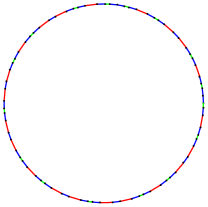
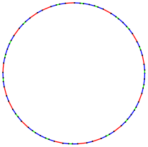
(a) $\eta_{1}$	(b) $\eta_{2}$	(c) $\eta_{3}$ [b]
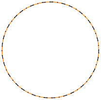
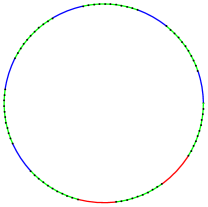
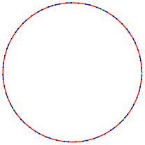
(d) $\eta_{4}$	(e) $\pi$	(f) $\eta_{5}$ [b]
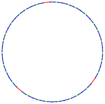
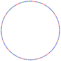
(g) $\eta_{6}$	(h) $\eta_{7}$	(i) $\eta_{8}$

Figure 2. The partition of $S^{1}$ for nine values of $\theta$ with $m=75$. Note that for (e), the partition is far less uniform than in the other figures.

4. Proof of Theorem 3

Remark.

Let $\bowtie$ be the equivalence relation on $\mathcal{S}$ of $\theta\bowtie\upsilon$ iff $\theta\pm\upsilon\in\mathbb{Z}$. Clearly $\#(\mathcal{S}/\bowtie)=8$, and for $\theta,\upsilon\in\mathcal{S}$, $d_{\theta}(m)=d_{\upsilon}(m)$ iff $\theta\bowtie\upsilon$. Therefore, $f_{m}:(\mathcal{S}/\bowtie)\to\mathbb{R}^{+}$ with $f_{m}(\theta)=d_{\theta}(m)$ is well-defined. $\mathcal{S}/\bowtie$ has the convenient choice of representatives $\{\eta_{i}:i\in[8]\}$.

As a consequence of this remark, we treat $\mathcal{S}$ implicitly as $\mathcal{S}/\bowtie$ because of our primary concern with the context of $d_{\theta}(m)$. We now introduce some further notation.

Definition.

Define the functions $w:\mathbb{N}\to\mathcal{S}$ and $W:\mathcal{S}\times\mathbb{N}\to\mathbb{R}$ as

$$w(M) =\operatornamewithlimits{argmin}\limits_{\theta\in\mathcal{S}}D_{M}(\theta)$$

$$W_{\theta}(M) =\#\{m\in[M]:\theta=w(m)\}.$$

We have the shorthand

$$LI(i) =\liminf\limits_{M\to\infty}\frac{W_{\eta_{i}}(M)}{M}$$

$$LS(i) =\limsup\limits_{M\to\infty}\frac{W_{\eta_{i}}(M)}{M}.$$

We now begin our approach towards Theorem 3. It is an immediate corollary to the following:

Theorem 11.

We have the following asymptotics, where the third and fifth column the give the percentages rounded to the nearest tenth:

$$\begin{array}[]{c||c|r||c|r||}i&\lx@intercol\hfil LI(i)\hfil\lx@intercol\vrule\lx@intercol\vrule\lx@intercol&\lx@intercol\hfil LS(i)\hfil\lx@intercol\vrule\lx@intercol\vrule\lx@intercol\\ \hline\cr\hline\cr 1&\frac{4\sqrt{5}-6}{11}&26.8&\frac{13+\sqrt{5}}{41}&37.2\bigstrut\\ \hline\cr 2&\frac{7-2\sqrt{5}}{29}&8.7&\frac{2-3\sqrt{5}}{11}&13.4\bigstrut\\ \hline\cr 3&9-4\sqrt{5}&5.6&\frac{7-2\sqrt{5}}{29}&8.7\bigstrut\\ \hline\cr 4&\frac{11-3\sqrt{5}}{38}&11.3&\frac{3\sqrt{5}-5}{10}&17.1\bigstrut\\ \hline\cr 5&\frac{19-8\sqrt{5}}{41}&2.7&\frac{12-5\sqrt{5}}{19}&4.3\bigstrut\\ \hline\cr 6&\frac{7\sqrt{5}-15}{10}&6.5&\frac{13-3\sqrt{5}}{62}&10.1\bigstrut\\ \hline\cr 7&\frac{4-\sqrt{5}}{11}&16.0&\sqrt{5}-2&23.6\bigstrut\\ \hline\cr 8&\frac{27-11\sqrt{5}}{62}&3.9&\frac{17-7\sqrt{5}}{22}&6.1\bigstrut\\ \hline\cr\end{array}$$

In particular, each of the $\liminf$s is positive.

As an illustration of the alternating nature for small $M$, see Figure 3, where if $\eta_{i}=\operatornamewithlimits{argmin}\limits_{\theta\in\mathcal{S}}D_{M}(\theta)$ then the $M$th data point $\left(M,\min\limits_{\theta\in\mathcal{S}}D_{M}(\theta)\right)$ is colored with the $i$th color in the following list: red, orange, purple, green, blue, brown, black, aquamarine. The code used to generate this figure can be found in §5.3.

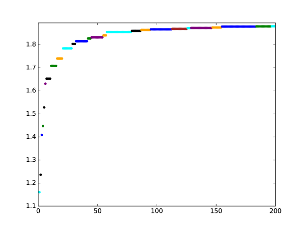
Figure 3. A plot of $\min\limits_{\theta\in\mathcal{S}}D_{M}(\theta)$ for $M\in[200]$, colored corresponding to $\operatornamewithlimits{argmin}\limits_{\theta\in\mathcal{S}}D_{M}(\theta)$.

The proof of this Theorem involves indirectly computing particular values of $W$ by computing the values at which each $\theta\in\mathcal{S}$ is the minimizer, in terms of the convergents. It is now convenient to look at the convergents as functions $k_{5},k_{6}:\mathcal{S}\to\mathbb{N}$:

$$k_{5}(\eta_{1}) =43 k_{6}(\eta_{1}) =70$$

$$k_{5}(\eta_{2}) =23 k_{6}(\eta_{2}) =37$$

$$k_{5}(\eta_{3}) =35 k_{6}(\eta_{3}) =57$$

$$k_{5}(\eta_{4}) =18 k_{6}(\eta_{4}) =29$$

$$k_{5}(\eta_{5}) =27 k_{6}(\eta_{5}) =44$$

$$k_{5}(\eta_{6}) =19 k_{6}(\eta_{6}) =30$$

$$k_{5}(\eta_{7}) =13 k_{6}(\eta_{7}) =21$$

$$k_{5}(\eta_{8}) =19 k_{6}(\eta_{8}) =31$$

We then define new sequences

$$K_{n}(1) =70F_{n}+43F_{n-1}$$

$$K_{n}(2) =71F_{n}+44F_{n-1}$$

$$K_{n}(3) =76F_{n}+47F_{n-1}$$

$$K_{n}(4) =79F_{n}+49F_{n-1}$$

$$K_{n}(5) =81F_{n}+50F_{n-1}$$

$$K_{n}(6) =89F_{n}+55F_{n-1}$$

$$K_{n}(7) =92F_{n}+57F_{n-1}$$

$$K_{n}(8) =97F_{n}+60F_{n-1}$$

with the further convention that for any $n\in\mathbb{N}$, $m\in\mathbb{Z}$, and $i\in[8]$,

$$K_{n}(i+8m)=K_{n-m}(i).$$

So, for instance, $K_{n}(0)=K_{n-1}(8)$.

Note that this is merely a reindexing of each $k_{n}(\cdot)$ by the permutation $\pi=(2\ 8\ 5)(3\ 7\ 6\ 4)\in S_{8}$ (that is, $K_{n}(j)$ is a shift of the convergents $k_{n}(\eta_{i})$ for $j=\pi i$). Call $\reflectbox{\rotatebox[origin={c}]{180.0}{$\pi$}}=\pi^{-1}$.

Lemma 12.

For all positive integers $n$,

$$K_{n}(1)<K_{n}(2)<K_{n}(3)<K_{n}(4)<K_{n}(5)<K_{n}(6)<K_{n}(7)<K_{n}(8)<K_{n+1}(1).$$

Proof.

Equivalently, $K_{n}(i)<K_{n}(j)<K_{n+1}(i)$ for all $1\leqslant i<j\leqslant 8$. The first inequality is obvious: if $K_{n}(i)=a_{i}F_{n}+b_{i}F_{n-1}$, then by inspection, $a_{i}<a_{j}$ whenever $i<j$. The second inequality comes from observing that $K_{n+1}(i)=a_{i}F_{n+1}+b_{i}F_{n}=(a_{i}+b_{i})F_{n}+a_{i}F_{n-1}$ and since $a_{i}>b_{j}$ for all $i,j$. ∎

Lemma 13.

Define the sequences $\sigma_{n}(i)$ and $\tau_{n}(i)$, where $\sigma_{n}(i)<\tau_{n}(i)<\sigma_{n+1}(i)-1$, as follows:

$$\{M\in\mathbb{N}:\eta_{i}=w(M)\}=\bigsqcup\limits_{n\in\mathbb{N}}[\sigma_{n}(i),\tau_{n}(i)].$$

Then, we have that $j=\pi i$ and

$$\sigma_{n}(i) =\left\lceil(K_{n+3}(j-2)-3)\left(\frac{K_{n-1}(j-1)+K_{n}(j-1)\varphi}{K_{n-1}(j-2)+K_{n}(j-2)\varphi}\right)\right\rceil-1$$

$$\tau_{n}(i) =\left\lceil(K_{n+3}(j-1)-3)\left(\frac{K_{n-1}(j)+K_{n}(j)\varphi}{K_{n-1}(j-1)+K_{n}(j-1)\varphi}\right)\right\rceil-2.$$

Proof.

We first establish that these sequences are well-defined for all $i$. $w(M)$ is $\eta_{i}$ for which $D_{M}(\eta_{i})<D_{M}(\eta_{j})$ for all $j\neq i$. However, for all choices of $i\neq j$ and $n$, with $M_{n}(i)=K_{n}(\pi i)+2K_{n+1}(\pi i)-2=K_{n+3}(\pi i)-2$, we have

$$D_{M_{n}(i)}(\eta_{i})\geqslant(M_{n}(i)+1)d_{\eta_{i}}(M_{n}(i))>D_{M_{n}(i)}(\eta_{j}).$$

The first inequality is trivial. The second follows by considering $m+1$ and $d_{\eta_{j}}(m)$ separately: clearly on $m\in[M_{n}(i)]$, $m+1\leqslant M_{n}(i)+1$. Then, say for fixed $j$ that $K_{n+2}(\pi j)-1\leqslant M_{n}(i)\leqslant K_{n+3}(\pi j)-2$. By Lemma 12, $M_{n-1}(i)<K_{n+2}(\pi j)<M_{n}(i)$, from which we conclude that $K_{n}(\pi i)<K_{n}(\pi j)$. By Corollary 7, we have that

$$d_{\eta_{i}}(M_{n}(i)) =\frac{1}{K_{n-1}(\pi i)+K_{n}(\pi i)\varphi}$$

$$d_{\eta_{j}}(M_{n}(i)) =\frac{1}{K_{n-1}(\pi j)+K_{n}(\pi j)\varphi}$$

Therefore $d_{\eta_{i}}(M_{n}(i))>d_{\eta_{j}}(M_{n}(i))$, concluding the second inequality. Thus, there are infinitely many values $M$ (e.g. those of the form $M_{n}(i)$) at which $\eta_{i}\neq w(M)$. Hence $\sigma_{n}(i)$ and $\tau_{n}(i)$ are well-defined sequences for all $i$.

Further, it is evident from the above argument that the “order of succession” for $M$ sufficiently large, e.g. $M\geqslant K_{1}(1)=70$, is $\eta_{\reflectbox{\rotatebox[origin={c}]{180.0}{$\pi$}}i}$ for $i=1,2,\dots,8$ and repeating—that is, $w(M)=\eta_{1}$ for $M$ on some interval $[s_{1},s_{2}-1]$, followed by $w(M)=\eta_{2}$ on $[s_{2},s_{3}-1]$, etc., up to $w(M)=\eta_{8}$ on $[s_{8},s_{1}^{\prime}-1]$, and then this cycle repeats with $w(M)=\eta_{1}$ on $[s_{1}^{\prime},s_{2}^{\prime}-1]$. Therefore we just need to compare $\eta_{\reflectbox{\rotatebox[origin={c}]{180.0}{$\pi$}}i}$ against $\eta_{\reflectbox{\rotatebox[origin={c}]{180.0}{$\pi$}}(i-1)}$ and $\eta_{\reflectbox{\rotatebox[origin={c}]{180.0}{$\pi$}}(i+1)}$. See Figure 4 for an illustration of the interval-based behvaior.

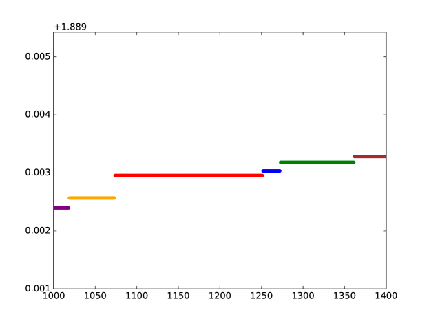
Figure 4. A plot of $\min\limits_{\theta\in\mathcal{S}}D_{M}(\theta)$ for $M\in[1200,1400]$, colored corresponding to $\operatornamewithlimits{argmin}\limits_{\theta\in\mathcal{S}}D_{M}(\theta)$.

It is now convenient to define “dual” sequences $\widehat{\sigma}_{n}(i)$ and $\widehat{\tau}_{n}(i)$ defined as $[\widehat{\sigma}_{n}(i),\widehat{\tau}_{n}(i)]\ni M$ the $n$th range on $\mathbb{N}\cap[70,\infty)$ for which $\eta_{\reflectbox{\rotatebox[origin={c}]{180.0}{$\pi$}}i}$ maximizes $D_{M}(\theta)$ over $\theta\in\mathcal{S}$. We see that for similar reasons, this maximizer cycles through $1,2,\dots,8$. We compute $\widehat{\sigma}_{n}(i)$ by considering $\eta_{\reflectbox{\rotatebox[origin={c}]{180.0}{$\pi$}}(i-1)},\eta_{\reflectbox{\rotatebox[origin={c}]{180.0}{$\pi$}}i}$: at what value $m>M_{n}(\reflectbox{\rotatebox[origin={c}]{180.0}{$\pi$}}(i-1))$ does it first occur that

$$(m+1)d_{\eta_{\reflectbox{\rotatebox[origin={c}]{180.0}{$\pi$}}i}}(m)\geqslant(M_{n}(\reflectbox{\rotatebox[origin={c}]{180.0}{$\pi$}}(i-1))+1)d_{\eta_{\reflectbox{\rotatebox[origin={c}]{180.0}{$\pi$}}(i-1)}}(M_{n}(\reflectbox{\rotatebox[origin={c}]{180.0}{$\pi$}}(i-1)))?$$

Algebraic manipulation gives $m\geqslant(M_{n}(\reflectbox{\rotatebox[origin={c}]{180.0}{$\pi$}}(i-1))-1)\left(\frac{K_{n-1}(\reflectbox{\rotatebox[origin={c}]{180.0}{$\pi$}}i)+K_{n}(\reflectbox{\rotatebox[origin={c}]{180.0}{$\pi$}}i)\varphi}{K_{n-1}(\reflectbox{\rotatebox[origin={c}]{180.0}{$\pi$}}(i-1))+K_{n}(\reflectbox{\rotatebox[origin={c}]{180.0}{$\pi$}}(i-1))\varphi}\right)$, hence

$$\widehat{\sigma}_{n}(i)=\left\lceil(M_{n}(\reflectbox{\rotatebox[origin={c}]{180.0}{$\pi$}}(i-1))-1)\left(\frac{K_{n-1}(\reflectbox{\rotatebox[origin={c}]{180.0}{$\pi$}}i)+K_{n}(\reflectbox{\rotatebox[origin={c}]{180.0}{$\pi$}}i)\varphi}{K_{n-1}(\reflectbox{\rotatebox[origin={c}]{180.0}{$\pi$}}(i-1))+K_{n}(\reflectbox{\rotatebox[origin={c}]{180.0}{$\pi$}}(i-1))\varphi}\right)-1\right\rceil.$$

Then, since $\mathbb{N}\cap[70,\infty)\subset\bigsqcup\limits_{n\in\mathbb{N}}\bigsqcup\limits_{i\in[8]}[\widehat{\sigma}_{n}(i),\widehat{\tau}_{n}(i)]$, we immediately obtain the relationship

$$\widehat{\tau}_{n}(i)=\widehat{\sigma}_{n}(i+1)-1.$$

Finally, we observe that

$$\sigma_{n}(i) =\widehat{\sigma}_{n}(\pi i-1)$$

$$\tau_{n}(i) =\widehat{\tau}_{n}(\pi i-1)=\widehat{\sigma}_{n}(\pi i)-1$$

because by that interval, all $j\neq i$ will have already achieved a maximum surpassing $\eta_{\reflectbox{\rotatebox[origin={c}]{180.0}{$\pi$}}i}$’s. ∎

Proof of Theorem 11.

Given $i$ and $M$, let $j=\pi i$ and let $n$ be the greatest integer such that $K_{n}(j)\leqslant M$. $W_{\eta_{i}}(M)\in\Theta\left(\tau_{n}(j)-\sigma_{n}(j)\right)$ and so we have the following asymptotic tendencies:

$$\liminf\limits_{M\to\infty}\frac{W_{\eta_{i}}(M)}{M} =\lim\limits_{n\to\infty}\frac{\tau_{n}(j)-\sigma_{n}(j)}{\sigma_{n+1}(j)-\sigma_{n}(j)}$$

$$\limsup\limits_{M\to\infty}\frac{W_{\eta_{i}}(M)}{M} =\lim\limits_{n\to\infty}\frac{\tau_{n}(j)-\sigma_{n}(j)}{\tau_{n}(j)-\tau_{n-1}(j)}$$

and using the exact values computed in Lemma 13 gives the stated values. ∎

We can interpret this result as saying that as $M$ grows, each element of $\mathcal{S}$ is represented as $w(M)$ infinitely many times. Further, $\eta_{1}=w(M)$ with marginally higher probability than the alternatives.

There is an interesting parallel to be drawn with Theorems 3 and 11 and with work in analytic number theory on prime distributions. In 1914, Littlewood [3] proved the unexpected fact that the difference $\pi(x)-\operatorname{li}(x)$ alternates infinitely often. Likewise, Theorem 3 gives eightfold (rather than twofold) alternation. Earlier, in 1853, Chebyshev noticed that $\pi(x,4,3)>\pi(x,4,1)$ despite the asymptotic behavior $\frac{\pi(x,4,3)}{\pi(x,4,1)}\to 1$, a result strengthened and generalized considerably by Rubinstein–Sarnak [8] and termed “Chebbyshev’s bias.” Here we see a much stronger emergent bias in the statement of Theorem 11, where there exists some $M_{0}\in\mathbb{N}$ where for all $M>M_{0}$, we have

$$W_{\eta_{1}}(M)>W_{\eta_{7}}(M)>W_{\eta_{4}}(M)>W_{\eta_{2}}(M)>W_{\eta_{6}}(M)>W_{\eta_{3}}(M)>W_{\eta_{8}}(M)>W_{\eta_{5}}(M).$$

In preliminary explorations that became this paper, an attempt was made at the related problem of

for each $M\in[49]$, minimize $D_{M}(\theta)$ over all $\theta\in\left[0,\frac{1}{2}\right]$.

The approach was to naïvely sample from the interval a large number of times (100000) for each $M$. Except when $M$ takes the values 30 and 31—where the optimum is approximately $\frac{1}{30}$ and $\frac{1}{31}$, respectively, to within one part in $10^{6}$—the values agree with the problem constrained for $\theta\in\mathcal{S}$ as is solved in this section of the text to within one part in at least $10^{3}$.

We can also compare these results with Ridley [7], which studies a related problem in packing efficiency of features in plants which grow at fixed divergence angles. There, the optimal angle (out of total angle 1) is determined to be $(\varphi-1)^{2}$; note that $\eta_{7}=(\varphi-1)^{2}$ (as enumerated in Figure 1). Therefore, we see that Ridley’s notion of optimality coincides with the notion explored here using $D_{M}(\theta)$ when $M$ takes the values 2, 5, 7–10, 29, 45, and 47–49, where in Ridley’s model, $M$ represents the number of generations, that is, the number of features (e.g. petals on a flower) that have grown using the constant divergence angle $\theta$.

5. Code

5.1. Python 2.7 code for the proof of Theorem 2

The following Python code was used following Lemma 10 to prove Theorem 2.

⬇

1phi = (1+5**0.5)/2

2rho = 1+2/5**0.5

3def V(n,a):

4 xl = [(a*i) % 1 for i in range(n+1)]

5 xl.sort()

6 xl.append(1)

7 maxGap = 0

8 for i in range(n+1):

9 if xl[i+1] - xl[i] > maxGap:

10 maxGap = xl[i+1] - xl[i]

11 return maxGap

12

13A = 18

14B = 18

15C = 14

16D = 12

17E = 11

18

19for a in range(1,A+1):

20 for b in range(1,B+1):

21 for c in range(1,C+1):

22 for d in range(1,D+1):

23 for e in range(1,E+1):

24 gt = [1,a,b,c,d,e,1,1,1,1,1,1,1,1,1,1,1, \

25 1,1,1,1,1,1,1,1,1,1,1,1,1,1,1,1]

26 xp = 1+1/(a+1/(b+1/(c+1/(d+1/(e+1/phi)))))

27 kcurr = 0

28 knext = 1

29 continueQ = True

30 for n in range(-1,30):

31 xp = 1./(xp-gt[n+1])

32 if n > 6:

33 xp = phi

34 for ga in range(0,gt[n+2]):

35 m = kcurr+(ga+2)*knext-2

36 if (m+1)*(xp-ga)/(knext*xp+kcurr) > rho:

37 continueQ = False

38 break

39 if not continueQ:

40 break

41 newknext = gt[n+2]*knext+kcurr

42 kcurr = knext

43 knext = newknext

44 if continueQ:

45 print a,b,c,d,e

5.2. Mathematica 12 code for generating Figure 2

The following Mathematica code was used to generate Figure 2.

Warning: due to internal precision error, the code sometimes crashes. The source of this error is in pos = Sort[N[DeleteDuplicates[Differences[L] // FullSimplify]]]; where DeleteDuplicates might leave a list of length longer than 3, in turn causing nearest3 to throw an error. This can be resolved manually for given a and n.

⬇

1nearest2[{a_, b_}][x_] := If[x < (a + b)/2, 1, 2];

2nearest3[{a_, b_, c_}][x_] := If[x < (a + b)/2, 1,

3 If[(a + b)/2 <= x < (b + c)/2, 2, 3]];

4tricolor[a_, n_] := Module[{L = Vlist[a, n], pos},

5 pos = Sort[N[DeleteDuplicates[Differences[L] // FullSimplify]]];

6 Table[{

7 If[Length[pos] == 2, {Black, Orange}[[

8 nearest2[pos][L[[i + 1]] - L[[i]]]]], {Green, Blue, Red}[[

9 nearest3[pos][L[[i + 1]] - L[[i]]]]]],

10 Thick, Circle[{0, 0}, 1, {2Pi L[[i]], 2Pi L[[i + 1]]}],

11 Black, Point[{Cos[2Pi L[[i]]], Sin[2Pi L[[i]]]}]

12 }, {i, 1, n + 1}]];

13

14Manipulate[Graphics[tricolor[a, n]], {n, 1, 100, 1},

15 {a, {(13 + Sqrt[5])/82 -> ”\!\(\*SubscriptBox[\(a\), \(1\)]\)”,

16 ( 7 - Sqrt[5])/22 -> ”\!\(\*SubscriptBox[\(a\), \(2\)]\)”,

17 (11 + Sqrt[5])/58 -> ”\!\(\*SubscriptBox[\(a\), \(3\)]\)”,

18 ( 5 - Sqrt[5])/10 -> ”\!\(\*SubscriptBox[\(a\), \(4\)]\)”,

19 ( 9 + Sqrt[5])/38 -> ”\!\(\*SubscriptBox[\(a\), \(5\)]\)”,

20 (25 - Sqrt[5])/62 -> ”\!\(\*SubscriptBox[\(a\), \(6\)]\)”,

21 ( 3 - Sqrt[5])/ 2 -> ”\!\(\*SubscriptBox[\(a\), \(7\)]\)”,

22 ( 7 + Sqrt[5])/22 -> ”\!\(\*SubscriptBox[\(a\), \(8\)]\)”}}]

5.3. Python 2.7 code for generating Figure 3

The following Python code was used to generate Figure 3. It is admittedly not the most efficient way to handle this data, but given the relatively small numbers used, ease of coding took priority over asymptotic efficiency.

V and rho are as in §5.1.

In order to produce an output on a different range $[a,b]$ of $x$-axis values (such as in Figure 4), replace the outer loop with for m in range(1,b+1) and the last line with plt.xlim(a,b).

⬇

1import matplotlib.pyplot as plt

2from math import sqrt

3etas = [ (13+sqrt(5))/82, (7-sqrt(5))/22, (11+sqrt(5))/58, (5-sqrt(5))/10, (9+sqrt(5))/38, (25-sqrt(5))/62, (3-sqrt(5))/2, (7+sqrt(5))/22 ]

4colors = [”red”,”orange”,”purple”,”green”,”blue”,”brown”,”black”,”aqua”]

5Vs = [[],]*8

6

7for m in range(1,201):

8 min = rho

9 minAt = 8

10 for i in range(8):

11 Vs[i] = Vs[i] + [(m+1)*V(m,etas[i])]

12 if max(Vs[i]) < min:

13 min = max(Vs[i])

14 minAt = i

15 plt.scatter([m],[min],c=colors[minAt],linewidths=0)

16plt.ylim(top=rho)

17plt.xlim(0,200)

References

- [1] R. L. Graham and J. H. van Lint. “On the Distribtion of modulo 1.” In: Can. J. Math. 20 (1966), pp. 1020–1024.
- [2] G. H. Hardy and E. M. Wright. An Introduction to the Theory of Numbers. Oxford University Press, 1938. ISBN: 9780199219865.
- [3] J. E. Littlewood. “Sur la distribution des nombres premiers.” In: Comptes Rendus 158 (1914), pp. 1869–1872.
- [4] C. J. Mozzochi. “A Proof of Sarnak’s Golden Mean Conjecture.” In: J. Number Theory (2020), to appear.
- [5] F. Motta, P. Shipman, and B. Springer. “Optimally Topologically Transitive Orbits in Discrete Dynamical Systems.” In: Am. Math. Mon. 123(2) (2016), pp. 115–135.
- [6] O. Parzanchevski and P. Sarnak. “Super-Golden-Gates for .” In: Adv. Math. 327 (2018), pp. 869–901.
- [7] J. N. Ridley. “Descriptive Phyllotaxis on Surfaces with Circular Symmetry.” In: Math Model 8 (1987), pp. 751–755.
- [8] M. Rubinstein and P. Sarnak. “Chebyshev’s bias.” In: Experiment. Math. 3(3) (1994), pp. 173–197.
- [9] N. Slater. “The distribution of the integer for which .” In: Proc. Cambridge Philos. Soc. 46 (1950), pp. 525–537.
- [10] V. Sós. “On the theory of diophantine approximations I.” In: Acta Math. 8 (1957), pp. 461–472.
5. Code