Storyboard: Optimizing Precomputed Summaries for Aggregation

Abstract.

An emerging class of data systems partition their data and precompute approximate summaries (i.e., sketches and samples) for each segment to reduce query costs. They can then aggregate and combine the segment summaries to estimate results without scanning the raw data. However, given limited storage space each summary introduces approximation errors that affect query accuracy. For instance, systems that use existing mergeable summaries cannot reduce query error below the error of an individual precomputed summary. We introduce Storyboard, a query system that optimizes item frequency and quantile summaries for accuracy when aggregating over multiple segments. Compared to conventional mergeable summaries, Storyboard leverages additional memory available for summary construction and aggregation to derive a more precise combined result. This reduces error by up to 25$\times$ over interval aggregations and 4.4$\times$ over data cube aggregations on industrial datasets compared to standard summarization methods, with provable worst-case error guarantees.

1. Introduction

An emerging class of data systems precompute aggregate summaries over a dataset to reduce query times. These precomputation (AggPre (Peng et al., 2018)) systems trade off preprocessing time at data ingest to avoid scanning the data at query time. In particular, Druid and similar systems partition datasets into disjoint segments and precompute summaries for each segment (Yang et al., 2014; Im et al., 2018). They can then process queries by aggregating results from the segment summaries. Unlike traditional data cube systems (Gray et al., 1997), the summaries go beyond scalar counts and sums and include data structures that can approximate quantiles and frequent items (Cormode et al., 2012). As an example, our collaborators at Microsoft often issue queries to estimate 99th percentile request latencies over hours-long time windows. Their Druid-like system precomputes quantile summaries (Dunning and Ertl, 2019; Gan et al., 2018) for 5 minute time segments and then combines summaries to estimate quantiles over a longer window, reducing data access and runtime at query time by orders of magnitude (Ray, 2013).

Although querying summaries is more efficient than querying raw data, precomputing summaries also limits query accuracy. Given a total storage budget and many data segments, each segment summary in an AggPre system has limited storage space – often <$10$ kilobytes – and thus limited accuracy (dru, 2020). Prior work on mergeable summaries introduces summaries that can be combined with no loss in accuracy, and are commonly used in AggPre systems (Agarwal et al., 2012; Gan et al., 2018; Ray, 2013). However, even mergeable summaries have maximum accuracy capped by the accuracy of an individual summary.

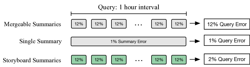
Figure 1. Given a space budget, mergeable summaries preserve accuracy when combined but cannot match the accuracy of using a single larger summary. Storyboard closes the gap by optimizing summaries for accurate aggregations.

We illustrate this challenge in Figure 1. Consider a query for the 99th percentile latency from 1:05pm to 2:05pm, and suppose we precompute mergeable quantile summaries for 5 minute time segments that individually have $12\%$ error. Calculating quantiles over the full hour requires aggregating results from $12$ summaries, and mergeable summaries would maintain $12\%$ error for the final result. This is not ideal: if the same space were instead used to store a single large summary for the entire interval, we would have $12\times$ less error with $\epsilon=1\%$. On the other hand, using a single large summary restricts the granularity of possible queries.

In this paper we introduce Storyboard, an AggPre query system that optimizes frequent items and quantile summaries for aggregation. Unlike mergeable summaries, Storyboard queries that combine results from multiple summaries have lower relative error than any summary individually. To do so Storyboard uses a different resource model than most existing summaries were designed for. While mergeable summaries assume the amount of memory available for constructing and aggregating (combining) summaries is the same as that for storage, we have seen in real-world deployments that AggPre systems have orders of magnitude more memory for construction and aggregation. Storyboard takes advantage of these additional resources to construct summaries that compensate for the errors in other summaries they may be combined with, and then aggregate results using a large and precise accumulator.

Storyboard focuses on supporting queries over intervals and data cubes roll-ups. Interval queries aggregate over one-dimensional contiguous ranges, such as a time window from 1:00pm to 9:00pm (Basat et al., 2018), while data cube queries aggregate over data matching specific dimension values, such as loc=USA AND type=TCP (Gray et al., 1997). When aggregating $k$ summaries together, Storyboard can reduce relative error by nearly a factor of $k$ for interval aggregations and a factor of $\sqrt{k}$ for other aggregations, compared with no reduction in error for mergeable summaries. These two query types cover a wide class of common queries and Storyboard can construct summaries optimized for either of the two types.

Interval Queries. For interval queries, Storyboard uses novel summarization techniques which we call cooperative summaries. Cooperative summaries account for the cumulative error over consecutive sequences of summaries, and adjust the error in new summaries to compensate. For instance, if five consecutive item frequency (heavy hitters) summaries have tended to underestimate the true frequency of item $x$, cooperative summaries can bias the next summary to overestimate $x$. This keeps the total error for queries spanning $k$ segments smaller than existing summarization techniques. Hierarchical approximation techniques (Basat et al., 2018; Qardaji et al., 2013) can also be used here but require additional space and provide worse accuracy in practice.

We prove that our summaries have cumulative error no worse than state of the art randomized summaries (Zengfeng Huang et al., 2011), and for frequencies exceed the accuracy of state of the art hierarchical approaches (Basat et al., 2018). Empirically, cooperative summaries provide a 4-25$\times$ reduction in error on queries aggregating multiple summaries compared with existing sketching and summarization techniques.

Multi-dimensional Cube Queries. Data cube queries can aggregate the same summary along different dimensions, so compensating for errors explicitly along a single dimension is insufficient. Instead, for cube workloads Storyboard used randomized weighted samples and reduces error further by optimizing for an expected workload of queries. Storyboard exploits the fact that data cubes often have dimensions with skewed value distributions: some values or combination of values that occur far more frequently than others. Then, Storyboard optimizes the allocation of storage space and introduces targeted biases where they will have the greatest impact to minimize average query error. Empirically, these optimizations yield an up to $4.4\times$ reduction in average error compared with standard data cube summarization techniques.

In summary, we make the following contributions:

1. We introduce Storyboard, an approximate AggPre system that provides improved query accuracy for aggregations by taking advantage of additional memory resources at data ingest and query time.

2. We develop cooperative frequency and quantile summaries that minimize error when aggregating over intervals and establish worst-case bounds on their error.

3. We develop techniques for allocating space and bias among randomized summaries to minimize average error under cube aggregations.

The remainder of the paper proceeds as follows. In Section 2 we provide motivating context. In Section 3 we present Storyboard and its query model. In Section 4 we describe cooperative summaries optimized for intervals. In Section 5 we describe optimizations for data cubes. In Section 6 we evaluate Storyboard’s accuracy. We describe related work in Section 7 and conclude in Section 8.

2. Background

Storyboard targets aggregation queries common in monitoring and data exploration applications, and improves accuracy for these queries by taking advantage of memory resources that real world summary precomputation systems already have available at query and ingest time. This motivation comes out of our experience collaborating with engineers at Imply, the developers of Druid, as well as a cloud services team at Microsoft.

Aggregation Queries. Existing usage of AggPre systems feature queries that span many segment summaries but follow structured patterns. At a cloud services team at Microsoft, users interacted with a Druid-like system primarily through a time-series monitoring dashboard which they used to track trends and explore anomalies. In addition to count and average queries, Top-K (heavy hitters) item frequency and quantile queries were prevalent. The most common forms of aggregations were over time intervals and grouped cube roll-ups. For instance, engineers often wanted to see the most common ip address frequencies over specific release windows or server configurations.

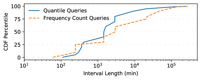
Figure 2. Distribution of user-issued time interval queries to a Druid-like system at Microsoft. More than half of the queries span $>100$ five-minute segments.

Notably, the queries over time intervals and data cubes involved combining results from a large number of summaries. In Figure 2 we describe a set of 33K Top-K item frequency queries and 130K quantile queries issued to an AggPre system at Microsoft. More than half of the queries span intervals longer than a day. Since the system stored summaries at a 5 minute granularity, this meant combining results from hundreds of summaries or reverting to less accurate, coarser grained roll-ups. Data cube roll-ups were also common. Users would commonly issue queries that filtered or grouped on a dimension, and “drill-down” (Gray et al., 1997) as needed, sometimes as part of anomaly explanation systems like MacroBase (Abuzaid et al., 2018b; Abuzaid et al., 2018a). Over 50% of all cubes had more than 10K dimension value segments and queries that span hundreds of cube segments were common.

Storyboard thus optimizes for the accuracy of time interval and cube queries that span not just a single summary, but aggregate over many summaries.

Memory Constraints. At both Imply and Microsoft, the storage space available to each summary was limited. Since summaries are maintained for each of potentially millions of segments, and nodes have limited memory and cache, the memory must be divided amongst the segment summaries. To illustrate, by default each quantile summary in Druid is configured for $2\%$ error and roughly 10 kB of memory usage (dru, 2020). Thus it is important to use summaries that provide high accuracy with minimal storage overhead. However, in real-world deployments there is much more memory available during summary construction and aggregation than there is for storage. For instance, in Druid the use of Hadoop map-reduce jobs for batch data ingestion allows for effectively unconstrained memory limits during summary construction. Then, at query time, engineers at Imply report that a standard deployment uses query processing jobs with $0.5$ GB of memory each when aggregating summaries together.

While standard mergeable summaries (Agarwal et al., 2012) are designed to maintain the same memory footprint during construction and aggregation that they use in storage, Storyboard takes advantage of additional memory at both construction and query time to achieve higher query accuracy.

3. System Design

In this section we describe Storyboard’s system design. We discuss the types of queries supported, how summaries are constructed for different query types, and how summaries are aggregated to provide accurate query results. We outline the system components in Figure 3.

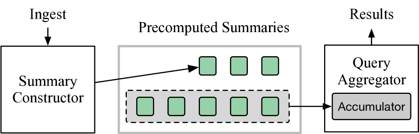
Figure 3. Storyboard precomputes summaries at ingest optimized to minimize error under aggregations. At query time, results from multiple summaries are combined using a precise accumulator to provide accurate results.

3.1. Queries

Consider data records $\rho=(x,t,d_{1},\dots,d_{m_{d}})$ where $x$ is either a categorical or ordinal value of interest (i.e. ip address, latency), $t$ is an ordered dimension for interval queries (i.e. timestamp), and the $d_{j}$ are categorical dimensions (i.e. location). A Storyboard query $g_{\mathcal{Q}}(x)$ specifies an aggregation of records $\mathcal{Q}$ and a function $g$ to estimate for the value $x$. $\mathcal{Q}$ defines an aggregation with a selection condition: either a one-dimensional interval or a multi-dimensional cube query (Basat et al., 2018; Gray et al., 1997).

Definition 1.

An interval aggregation specifies $\mathcal{Q}^{\text{(time)}}=\{\rho:T_{0}\leq t<T_{1}\}$ for $T_{0},T_{1}$ aligned at a time-resolution $T_{G}$ ($T_{0},T_{1}\bmod T_{G}=0$) and maximum length $T_{1}-T_{0}\leq k_{T}\cdot T_{G}$.

Definition 2.

A data cube aggregation specifies $\mathcal{Q}^{\text{(cube)}}=\{\rho:d_{i_{1}}=v_{i_{1}}\wedge\dots\ \wedge d_{i_{k}}=v_{i_{k}}\}$ for $d_{i_{1}},\dots,d_{i_{k}}$ a subset of the dimensions to condition on.

The query function $g$ is either an item frequency $f$ or rank $r$ (Cormode and Hadjieleftheriou, 2010; Luo et al., 2016). An item frequency $f(x)$ is the total count of records with value $x$ while a rank $r(x)$ is the total count of records with values less than or equal to $x$. We use $g$ generically denote either frequencies or ranks.

(1) $$f_{\mathcal{Q}}(x)=\sum_{\rho_{i}\in\mathcal{Q}}1_{x_{i}=x}\qquad\qquad r_{\mathcal{Q}}(x)=\sum_{\rho_{i}\in\mathcal{Q}}1_{x_{i}\leq x}.$$

Using these primitives, Storyboard can also return estimates for quantiles and Top K / Heavy Hitters queries, which we will discuss in more detail in Section 3.3.

3.2. Data Ingest

Before Storyboard can ingest data, users specify whether they want the dataset to support interval or data cube aggregations, and whether they want the dataset to support frequency or rank query functions. Users also specify total space constraints and workload parameters. A dataset can be loaded multiple times to support different combinations of the above.

Storyboard then splits the data records into atomic segments $\mathcal{D}$. These segments form a disjoint partitioning of a dataset, and are chosen so that any aggregation can be expressed as a union of segments. For interval aggregations users specify a time resolution $T_{G}$ and a maximum length $k_{T}$, defining segments $\mathcal{D}_{i}=\{\rho:i\cdot T_{G}\leq t<(i+1)\cdot T_{G}\}$ For cube aggregations the partitions are defined by grouping by all $m_{d}$ of the dimensions $\mathcal{D}_{\vec{v}}=\{\rho:d_{1}=v_{1}\wedge\dots\wedge d_{m_{d}}=v_{m_{d}}\}$. Once the dataset is partitioned we can represent the records in each segment as mappings from values to counts:

$$\mathcal{D}=\{x_{1}\mapsto\delta_{1},\dots,x_{r}\mapsto\delta_{r}\}.$$

For each segment $\mathcal{D}$ Storyboard constructs a summary $S$ consisting of $s$ value, count mappings

$$S\coloneqq\{x_{1}\mapsto\gamma_{1},\dots,x_{s}\mapsto\gamma_{s}\}.$$

This is similar to other counter based summaries (Metwally et al., 2005; Cormode and Hadjieleftheriou, 2010) and weighted sampling summaries (Zengfeng Huang et al., 2011). Unlike tabular sketches such as the Count-Min Sketch (Cormode and Muthukrishnan, 2005) Storyboard summaries include the values $x$. We assume we have enough memory and compute to generate $S$, making our routines closer to coreset construction (Phillips, 2017) than streaming sketches (Muthukrishnan et al., 2005). More details on how the values $x$ and counts $\gamma$ are chosen for each summary are given in Section 4.1 for interval aggregations and Section 5.1 for cube aggregations.

3.3. Query Processing

After the summaries have been constructed, the Storyboard query processor can return query estimates $\hat{g}_{\mathcal{Q}}(x)$ for different aggregations $\mathcal{Q}$ by using the summaries $S_{i}$ as proxies for the segments $\mathcal{D}_{i}$. Then, using $g$ to denote a generic query function, we can derive frequency or rank estimates over a query aggregation $\mathcal{Q}$ by adding up the estimates for the segment summaries.

$$f_{S}(x)\coloneqq\sum_{x_{j}\in S}\gamma_{j}\cdot 1_{x_{j}=x}\qquad r_{S}(x)\coloneqq\sum_{x_{j}\in S}\gamma_{j}\cdot 1_{x_{j}\leq x}$$

(2) $$\hat{g}_{\mathcal{Q}}(x)=\sum_{S_{i}\in\mathcal{Q}}g_{S_{i}}(x)$$

For single rank or frequency estimates $\hat{g}_{\mathcal{Q}}(x)$ the query processor can precisely add up scalar estimates using Equation 2. This is more efficient than merging mergeable summaries (Agarwal et al., 2012), since we are just accumulating scalars, and potentially more accurate as we will discuss in Section 3.4.

Storyboard uses a richer accumulator data structure $A$ to support quantile and top-k / heavy hitter queries. When there is sufficient memory, $A$ tracks the proxy values and counts in $S_{1},\dots,S_{k}$. We then sort the items in $A$ by value to estimate quantiles or by count to estimate heavy hitters. When memory is constrained, we instead let $A$ be a standard but very large stream summary of the proxy values and counts stored in $S_{1},\dots,S_{k}$. We specifically use a Space Saving sketch (Metwally et al., 2005) for heavy hitters and a PPS (VarOpt (Cohen et al., 2011)) sample for quantiles. Then we can query $A$ to get quantile or heavy hitters estimates. In practice the space $s_{A}$ available to $A$ is orders of magnitude greater than the space $s$ available to any precomputed summary, i.e. 50,000$\times$ in the deployment described in Section 2.

3.4. Error Model

Consider the absolute (i.e. unscaled) error $\varepsilon_{\mathcal{Q}}$ which is the difference between the true and estimated item frequency counts, or the difference between the true and estimated ranks for a query aggregation $\mathcal{Q}$. Throughout the paper, we will use absolute errors $\varepsilon$ for analysis, when comparing final query quality we use the relative (scaled) error ${\epsilon^{\prime}}=\varepsilon/|\mathcal{Q}|$ (Cormode and Hadjieleftheriou, 2010) where $|\mathcal{Q}|=\sum_{\rho_{i}\in\mathcal{Q}}1$.

When accumulating scalar rank or frequency estimates directly using Equation 2 the error $\varepsilon_{\mathcal{Q}}(x)$ is just the sum of the errors introduced by the segment summaries for $\mathcal{Q}$:

(3) $$\varepsilon_{\mathcal{Q}}(x)=\sum_{\mathcal{D}_{i}\in\mathcal{Q}}\varepsilon_{\mathcal{D}_{i}}(x)=\sum_{\mathcal{D}_{i}\in\mathcal{Q}}\left(g_{\mathcal{D}_{i}}(x)-g_{S_{i}}(x)\right)$$

When using the accumulator $A$ a quantile or heavy hitter estimate will be based off the distribution defined by the $\hat{g}_{S}(x)$, but $A$ introduces its own additional error $\varepsilon^{\text{(A)}}_{S}$ in approximating the proxy values in the summaries $S$, yielding a total error of:

(4) $$\varepsilon^{\text{(A)}}_{\mathcal{Q}}(x)\leq|\varepsilon_{\mathcal{Q}}(x)|+|\varepsilon^{\text{(A)}}_{S}(x)|.$$

Furthermore we are interested in systems that provide error bounds over all values of $x$, so we consider the worst case error $\varepsilon^{\text{(A)}}_{\mathcal{Q}}\coloneqq\max_{x}|\varepsilon^{\text{(A)}}_{\mathcal{Q}}(x)|$. A bound on the maximum error over all $x$ also bounds the error of any quantile or heavy hitter frequency estimate derived from the raw estimates $\hat{g}$.

To analyze the error, consider an aggregation $\mathcal{Q}$ accumulating $k$ segments, each with total weight $n=|\mathcal{D}|=\sum_{x_{i}\in\mathcal{D}}\delta_{i}$ and represented using summaries of size $s$. Also, suppose that the accumulator $A$ has size $s_{A}\gg s$. Suppressing logarithmic factors, state of the art frequency and quantile summaries have absolute error $O(n/s)$ (Karnin et al., 2016; Cormode and Hadjieleftheriou, 2010; Agarwal et al., 2012; Phillips, 2017). Different summarization techniques yield different errors as the size of the aggregation $k$ grows. Storyboard can reduce relative error significantly for large $k$. We summarize the error bounds in Table 1.

Table 1. Summary Error ignoring constants combining $k$ summaries. The summaries used by storyboard: CoopQuant, CoopFreq, and PPS, all have reduced errors as for large $k$.

Summary	Relative ${\epsilon^{\prime}}_{\mathcal{Q}}$	Tot. Space
CoopFreq	${\log{k_{T}}}/({sk})+1/s_{A}$	$sk$
CoopQuant	$\sqrt{k_{T}}/({sk})+1/s_{A}$	$sk$
PPS (Cohen et al., 2011)	$1/(s\sqrt{k})+1/s_{A}$	$sk$
Mergeable (Agarwal et al., 2012)	$1/s$	$sk$
Uniform Sample	$1/\sqrt{sk}+1/s_{A}$	$sk$
Hierarchical (Basat et al., 2018; Qardaji et al., 2013)	$\log{k}/(sk)+1/s_{A}$	$sk\log{k_{T}}$

Using mergeable summaries (Agarwal et al., 2012) for both $S$ and the accumulator $A$ gives us maximum absolute error $\varepsilon^{\text{(merge)}}_{\mathcal{Q}}\leq O(|\mathcal{Q}|/s)\leq O(kn/s)$ and maximum relative error

(5) $${\epsilon^{\prime}}^{\text{(merge)}}_{\mathcal{Q}}\leq O(1/s).$$

Storyboard’s accumulator $A$ applied to standard summaries gives us in the worst case $\varepsilon^{\text{(A)naive}}_{\mathcal{Q}}\leq\sum_{\mathcal{D}_{i}\in\mathcal{Q}}|O(n/s)|+O(nk/s_{A})$ so

(6) $${\epsilon^{\prime}}^{\text{(A)naive}}_{\mathcal{Q}}\leq O(1/s)+O(1/s_{A})$$

where the $O(1/s_{A})$ is negligible for $s_{A}\gg s$.

However, Storyboard is able to achieve lower query error by reducing the sum of errors from summaries in Equation 3. By using independent, unbiased, weighted random samples – specifically PPS summaries in Section 5.1 – sums of random errors centered around zero will concentrate to zero, and one can use Hoeffding’s inequality to show that with high probability and ignoring log terms $\sum_{\mathcal{D}_{i}\in\mathcal{Q}}\varepsilon_{\mathcal{D}_{i}}(x)\leq O(\sqrt{k}n/s)$ so

(7) $${\epsilon^{\prime}}^{\text{(A)PPS}}_{\mathcal{Q}} \leq O\left(\frac{1}{\sqrt{k}{s}}\right)+O(1/s_{A}).$$

This already is lower than the relative error for mergeable summaries in Equation 5 for $k\gg 1$ and $s_{A}\gg s$.

In practice, Cooperative summaries (Section 4) achieve even better error than PPS summaries for interval queries. We can prove that cooperative quantile summaries satisfy $\max_{x}|\varepsilon_{\mathcal{Q}}^{(A)\texttt{Coop\-Quant}}(x)|\leq O(n\sqrt{k_{T}}/s)$

(8) $${\epsilon^{\prime}}_{\mathcal{Q}}^{(A)\texttt{Coop\-Quant}} \leq O\left(\frac{\min(\sqrt{k_{T}},k)}{ks}\right)+O(1/s_{A})$$

with much better empirical performance over intervals than PPS, while cooperative frequency summaries satisfy
$\max_{x}|\varepsilon_{\mathcal{Q}}^{(A)\texttt{Coop\-Freq}}(x)|\leq O(n\log{k_{T}}/s)$

(9) $${\epsilon^{\prime}}_{\mathcal{Q}}^{(A)\texttt{Coop\-Freq}} \leq O\left(\frac{\min(\log{k_{T}},k)}{ks}\right)+O(1/s_{A})$$

where $k_{T}$ is the maximum length of an interval. See Section 4.2 for more details and proof sketches.

Hierarchical estimation is a common solution for interval (range) queries (Basat et al., 2018; Cormode and Muthukrishnan, 2005) and show up in differential privacy as well (Cormode et al., 2019). We will describe an instance of these methods to illustrate their error scaling. A dyadic (base $2$) hierarchy stores summaries of size $s\cdot 2^{h}$ for $h=1\dots\log{k_{T}}$ to track segments of different lengths. They can thus estimate intervals of length $k$ with error $\varepsilon_{\mathcal{Q}}^{\text{(A)Hier}}\leq O(n\log{k}/s)+O(1/s_{A})$, similar to our cooperative frequency sketches. However, they incur an additional $\log{k_{T}}$ factor in space usage to maintain their multiple levels of summaries and provide worse error empirically than our Cooperative summaries.

4. Cooperative Summaries

In this section we describe the cooperative summarization algorithms Storyboard uses for interval queries. These summaries achieve high query accuracy when combined by compensating for accumulated errors over sequences of summaries.

4.1. Interval Summary Construction

For interval queries, we assume that users specify a space limit $s$ to use for summarizing an incoming data segment $\mathcal{D}$. Cooperative summaries then must make efficient use of their $s$ samples ($x_{i}\mapsto\gamma_{i}$) to accurately represent a local segment of data. To match state of the art summaries, we want

(10) $$\max_{x}|\hat{g}_{S}(x)-g_{\mathcal{D}}(x)|\leq r|\mathcal{D}|/s$$

for an accuracy parameter $r\geq 1$. However, there are many possible ways to choose the items to store in $S$ that would satisfy Equation 10.

Within these constraints, Storyboard can choose $x_{i},\gamma_{i}$ to minimize the total error for queries that aggregate multiple summaries. Storyboard explicitly minimizes the error over a set of queries with fixed start points every $k_{T}$ segments. We call these aggregation intervals “prefix” intervals $\text{Pre}_{t}$, a modification of standard prefix-sum ranges (Ho et al., 1997).

(11) $$\text{Pre}_{t}=\{\mathcal{D}_{k_{T}\lfloor t/k_{T}\rfloor},\dots,\mathcal{D}_{k_{T}\lfloor t/k_{T}\rfloor+t\bmod k_{T}}\}.$$

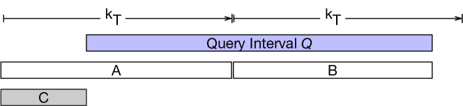
Figure 4. Any contiguous interval can be expressed as a linear combination of aligned intervals $\text{Pre}_{t}$. In this example, $Q$ is expressed as $A\cup B\setminus C$

Figure 4 illustrates how any consecutive interval of up to $k_{T}$ segments can be represented as an additive combination of up to $3$ prefix intervals. As long as prefix intervals have bounded error $\varepsilon_{\text{Pre}_{t}}=g_{\text{Pre}_{t}}-\hat{g}_{\text{Pre}_{t}}$, any contiguous interval up to length $k_{T}$ has error at most $3\varepsilon$. In order to minimize $\varepsilon_{\text{Pre}_{t}}(x)$ Storyboard will have to track its exact values, which may be resource intensive but is done during data ingest. The details of the summary construction algorithm differ for frequencies and ranks.

function CoopFreq($\mathcal{D}_{t},s$)

     $h\leftarrow|\mathcal{D}_{t}|/s$

     $\varepsilon_{\text{Pre}_{t}}(x)\leftarrow\varepsilon_{\text{Pre}_{t-1}}(x)+f_{\mathcal{D}_{t}}(x)$

     $S_{t}\leftarrow\{x\mapsto f_{\mathcal{D}_{t}}(x):f_{\mathcal{D}_{t}}(x)\geq h\}$ $\triangleright$ Heavy hitters

     while $|S_{t}|<s$ do $\triangleright$ Correct Accumulated Errors

         $x_{m}\leftarrow\arg\max_{x\in\text{Pre}_{t}\setminus S_{t}}\left(\varepsilon_{\text{Pre}_{t}}(x)\right)$

         $\delta_{m}\leftarrow\min\left(r\cdot h,\varepsilon_{\text{Pre}_{t}}(x)\right)$

         $S_{t}\leftarrow S_{t}\cup\{x_{m}\mapsto\delta_{m}\}$

         $\varepsilon_{\text{Pre}_{t}}(x)\leftarrow\varepsilon_{\text{Pre}_{t}}(x)-\delta_{m}\cdot 1_{x=x_{s}}$      

     return $S_{t}$

Algorithm 1 Cooperative Item Frequencies Summary

In Algorithm 1 we present pseudocode for constructing a cooperative summary of size $s$ for frequency estimates on a data segment $\mathcal{D}_{t}$. To satisfy Equation 10 and accurately represent $\mathcal{D}_{t}$, we store the true count for any segment-local heavy hitter items in $\mathcal{D}_{t}$ that occur with count greater than $|\mathcal{D}_{t}|/s$. The remaining space in the summary is allocated to compensating the $x$ with the highest cumulative undercount $\varepsilon_{\text{Pre}_{t}}(x)$ thus far so that overcounting $x$ in $S_{t}$ will adjust for the undercount in the other summaries going forward. For each of these compensating $x$, we store the smaller of $r|\mathcal{D}|/s$ and $\varepsilon_{\text{Pre}_{t}}(x)$. This ensures Equation 10 is satisfied and also keeps $\varepsilon_{\text{Pre}_{t}}(x)$ positive, a useful invariant for proofs later. Larger $r$ allow the algorithm trade off higher local error for less error accumulation across summaries.

function CoopQuant($\mathcal{D}_{t},s$)

     $h\leftarrow|\mathcal{D}_{t}|/s$; $S_{t}\leftarrow\{\}$

     $\varepsilon_{\text{Pre}_{t}}(x)\leftarrow\varepsilon_{\text{Pre}_{t-1}}(x)+r_{\mathcal{D}_{t}}(x)$

     $\mathcal{D}_{t1},\dots,\mathcal{D}_{ts}\leftarrow\textsc{Partition}(\mathcal{D}_{t},s)$ $\triangleright$ Sorted Chunks

     for $i\in 1\dots s$ do

         $L(z)\coloneqq\sum_{y\in U}\phi(\varepsilon_{\text{Pre}_{t}}(y))$

         $x_{s}\leftarrow\arg\min_{z\in\mathcal{D}_{ti}}L(z)$ $\triangleright$ Minimize Loss

         $S_{t}\leftarrow S_{t}\cup\{x_{s}\mapsto h\}$

         $\varepsilon_{\text{Pre}_{t}}(x)\leftarrow\varepsilon_{\text{Pre}_{t}}(x)-h\cdot 1_{x\geq x_{s}}$      

     return $S_{t}$

Algorithm 2 Cooperative Quantile Summary

In Algorithm 2 we present pseudocode for constructing a cooperative summary of size $s$ for rank estimates on a data segment $\mathcal{D}_{t}$. To satisfy Equation 10 and accurately represent $\mathcal{D}_{t}$, we sort the values in $\mathcal{D}$ and partition the sorted values into $s$ equally sized chunks. Then CoopQuant selects one value in each chunk to include in $S_{t}$ as a representative with proxy count $|\mathcal{D}|/s$. This ensures that the any rank can be estimated using $S_{t}$ with error at most $|\mathcal{D}|/s$. Within each chunk, we store the item that minimizes a total loss $L=\sum_{x\in U}\phi(\varepsilon_{\text{Pre}_{t}}(x))$ with $\phi(\epsilon)=\cosh{(\alpha\epsilon)}$, $\alpha=s/({\sqrt{k_{T}}n_{\text{max}}})$, $n_{\text{max}}=\max_{t}|\mathcal{D}_{t}|$ the maximum size of a data segment, and $k_{T}$ the maximum interval length. $\cosh(x)=\frac{1}{2}(e^{x}+e^{-x})$ is used in discrepancy theory (Spencer, 1977) to exponentially penalize both large positive and large negative errors, so $L$ serves as a proxy for the $L_{\infty}$ maximum error. Note that we need to bound $n_{\text{max}}$ to set $\alpha$ for this algorithm, though in practice accuracy changes very little depending on $n_{\text{max}}$

4.2. Interval Query Error

CoopFreq and CoopQuant both provide estimates with local error $\varepsilon_{\mathcal{D}}(x)\leq r|\mathcal{D}|/s$ for a single segment $\mathcal{D}$, and minimize the cumulative error over $\varepsilon_{\text{Pre}_{t}}(x)$ prefix intervals (and thus general intervals). In this section we analyze how $\varepsilon_{\text{Pre}_{t}}(x)$ grows with $t$. This allows us to prove Equations 8 and 9 in Section 3.4 which bound the query error from accumulating results over any sequence of $k_{T}$ summaries.

The general strategy will be to define a loss $L_{t}$ which is a function of the errors $\varepsilon_{\text{Pre}_{t}}(x)$ parameterized by a cost function $\phi$

(12) $$L_{t}\coloneqq\sum_{x\in U}\phi\left(\varepsilon_{\text{Pre}_{t}}(x)\right)$$

where $U$ is the universe of observed values $x\in|\text{Pre}_{t}|$. We can bound the growth of $L_{t}$ when CoopQuant and CoopFreq are used to construct sequences of summaries. Then, we can relate $L_{t}$ and $\max_{x}|\varepsilon_{\text{Pre}_{t}}(x)|$ to bound the latter. Omitted proofs in this section can be found in Appendix A.

4.2.1. CoopFreq Error

For frequency summaries, we use the cost function $\phi(x)=\exp(\alpha x)$ for a parameter $\alpha$. We minimize a sum of exponentials as a proxy for the maximum error. Lemma 1 bounds how much $L_{t}$ can increase with $t$.

Lemma 0.

When CoopFreq constructs a summary with size $s$ for $\mathcal{D}_{t}$ the loss satisfies

$$L_{t}\leq L_{t-1}+\alpha r|\mathcal{D}_{t}|$$

for $\phi(x)=\exp(\alpha x)$ as long as $0<\alpha\leq 2\frac{s}{|\mathcal{D}_{t}|}\frac{r-1}{r^{2}}$.

Given this, we can bound the cumulative error:

Theorem 2.

CoopFreq maintains

$$\max_{x\in U}|\varepsilon_{\text{Pre}_{t}}(x)|\leq\frac{1}{\alpha}\ln\left(1+\alpha r\sum_{i=1}^{t}|\mathcal{D}_{i}|\right)$$

where $\alpha=2\frac{s}{\max_{i}{|\mathcal{D}_{i}|}}\frac{r-1}{r^{2}}$.

Proof.

$\alpha$ satisfies the conditions in Lemma 1 so $L_{t}\leq L_{0}+\alpha r\sum_{i=0}^{t}|\mathcal{D}_{i}|$ and thus

$$\exp(\alpha\max_{x\in U}\varepsilon_{t}(x))-1\leq\alpha r\sum_{i=0}^{t}|\mathcal{D}_{i}|$$

∎

To illustrate the asymptotic behavior we can apply Theorem 2 with $r=\frac{3}{2}$ and consistent segment weights $n=|\mathcal{D}_{i}|$ to see in Corrollarry 1 that the absolute error grows logarithmically with the number of segments $k$ in the interval.

Corollary 1.

For $r=\frac{3}{2}$ and $|\mathcal{D}_{i}|=n$, CoopFreq maintains

$$\max_{x\in U}|\varepsilon_{k}(x)|\leq\frac{9}{4}\frac{n}{s}\ln\left(1+\frac{2}{3}nk\right)$$

In fact this result is close to optimal: an adversary generating incoming data can guarantee at least $\Omega(\log{k})$ error accumulation by generating data containing items the summaries have undercounted the most so far.

4.2.2. CoopQuant Error

For rank queries we use the cost function $\phi(x)=\cosh{\alpha x}$. Since $\cosh{z}=\frac{1}{2}(\exp(z)+\exp(-z))$ this exponentially penalizes both under and over-estimates symmetrically, and is thus a smooth proxy for the maximum absolute error of the error, also used in discrepancy theory (Spencer, 1977). As with CoopFreq, Lemma 3 bounds how much $L_{t}$ can increase with $t$.

Lemma 0.

When CoopQuant constructs a summary with size $s$ for $\mathcal{D}_{t}$ the loss function satisfies

$$L_{t}\leq L_{t-1}\exp{\alpha^{2}(|\mathcal{D}_{t}|/s)^{2}/2}$$

for $\phi(x)=\cosh(\alpha x)$

From Lemma 3 we can bound the maximum rank error.

Theorem 4.

CoopQuant maintains

$$\max_{x\in U}|\varepsilon_{\text{Pre}_{t}}(x)|\leq\frac{1+2\ln{(2|U|)}}{2s}\sqrt{\sum_{i}^{t}|\mathcal{D}|_{t}^{2}}$$

with $\phi(x)=\cosh(\alpha x)$ and $\alpha=s\left(\sum_{i=0}^{t}|\mathcal{D}_{i}|^{2}\right)^{-1/2}$.

Proof.

Using Lemma 3:

$$L_{t} \leq L_{0}\exp{\left(\alpha^{2}/2\sum_{i=0}^{t}\left(\frac{|\mathcal{D}_{i}|}{s}\right)^{2}\right)}$$

$$\max_{x\in U}|\varepsilon_{t}(x)| \leq\frac{1}{\alpha}\ln(2|U|)+\frac{\alpha}{2}\sum_{i=0}^{t}\left(\frac{|\mathcal{D}_{i}|}{s}\right)^{2}$$

Then setting $\alpha=s/{\sqrt{\sum_{i=0}^{t}|\mathcal{D}_{i}|^{2}}}$ completes the proof. ∎

This can be instantiated for data segments with constant total weight in Corrollary 2, which shows that CoopQuant has error $O(\sqrt{k}/s)$.

Corollary 2.

For $|\mathcal{D}_{t}|=n$ constant and $\phi(x)=\cosh(\alpha x)$ with $\alpha=\frac{s}{n\sqrt{k}}$, CoopQuant maintains

$$\max_{i\in U}|\varepsilon_{\text{Pre}_{k}}(i)|\leq\frac{n}{2s}\left(\sqrt{k}+2\ln{(2|U|)}\right)$$

5. Optimizing Cube Queries

In this section we describe the weighted probability proportional to size samples (PPS) (Cohen et al., 2011; Ting, 2018) Storyboard uses to summarize segments for both frequency and rank data cube aggregations. These randomized summaries have errors which cancel out with high probability. Then we describe how Storyboard optimizes the allocation of space and bias to these summaries to increase average query accuracy further for target cube workloads.

5.1. PPS Summaries

A PPS summary is a weighted random sample that includes items with probability proportional to their size or total count in a data segment $\mathcal{D}$ (Cohen et al., 2011; Ting, 2018; Zengfeng Huang et al., 2011). Values $x_{i}$ with true occurence count $\mathcal{D}(x_{i})=\delta_{i}$ are sampled for inclusion in the summary $S$ according to Equation 13

(13) $$\Pr[x_{i}\in S] =\min(1,\delta_{i}/h)$$

(14) $$S(x_{i}) =\begin{cases}h&\delta_{i}\leq h\\ \delta_{i}&\delta_{i}>h\end{cases}.$$

For an accuracy parameter $h$, heavy hitters that occur more than $h$ times are always sampled with their true count, while those with count $0\leq\delta_{i}\leq h$ are either included with a proxy weight of $h$ or excluded from the summary. Thus, $S(x_{i})$ is an unbiased estimate for $\delta_{i}$ with maximum local error of $h$. We will see later that rank estimates $\hat{r}_{S}(x)\sum_{x_{j}\in S}\gamma_{j}\cdot 1_{x_{j}\leq x}$ can also bounded by $h$.

Setting $h\leq|\mathcal{D}|/s$ ensures that the summary will have expected size $s$, but is conservative. In Algorithm 3 we present the procedure from (Cohen et al., 2011) we use to set $h$ to minimize error while keeping the summary size at most $s$ by excluding the effect of heavy hitters.

function CalcT($\mathcal{D},s$)

     $h\leftarrow|\mathcal{D}|/s$

     $H\leftarrow\{\}$ $\triangleright$ Local Heavy Hitters

     while $\max_{x\in\mathcal{D}\setminus H}f_{\mathcal{D}}(x)\geq h$ do

         $x_{\text{max}}\leftarrow\arg\max_{x\in\mathcal{D}\setminus H}\mathcal{D}(x)$

         $H\leftarrow H\cup\{x_{\text{max}}\}$

         $h\leftarrow\frac{\sum_{x\in\mathcal{D}\setminus H}f_{\mathcal{D}}(x)}{s-|H|}$      

     return $h$

Algorithm 3 Calculate minimal $h$ threshold

One way to implement PPS is to independently sample items according to Equation 13, but this does not guarantee the summary will store exactly $s$ values. Instead we use the PairAgg procedure in Algorithm 4 to transform sampling probabilities for pairs of items until we have $s$ or $s-1$ values with probability $1$. We can do so in a way that guarantees that the error $\max_{x}|\varepsilon(x)|\leq h$ and is unbiased with $E[\varepsilon(x)]=0$ for both frequency and rank queries. See (Cohen et al., 2011) for details.

function PairAgg($p_{i},p_{j}$)

    if $p_{i}+p_{j}<1$ then

         if $\text{rand}()<p_{i}/(p_{i}+p_{j})$ then $p_{i}\leftarrow p_{i}+p_{j}$; $p_{j}\leftarrow 0$

         else  $p_{j}\leftarrow p_{i}+p_{j}$; $p_{i}\leftarrow 0$          

    else

         if $\text{rand}()<\frac{1-p_{j}}{2-p_{i}-p_{j}}$ then $p_{i}\leftarrow 1$; $p_{j}\leftarrow p_{i}+p_{j}-1$

         else  $p_{i}\leftarrow p_{i}+p_{j}-1$; $p_{j}\leftarrow 1$              

Algorithm 4 Pair Aggregation for PPS

5.2. Cube Summary Construction

For data cubes, storyboard maintains a collection of PPS summaries for data segments $\mathcal{D}_{i}$ that form a complete, atomic partition of combinations of dimension values. A cube query then specifies a set of segments $\mathcal{Q}_{s}=\{\mathcal{D}_{1},\dots,\mathcal{D}_{k}\}$ that match dimension value filters. Storyboard ingests a complete cube dataset in batch and is given a total space budget $S_{T}$ for storing summaries. This opens up the opportunity for optimizations across the entire collection of summaries.

In most multi-dimensional data cubes some queries and dimension values will be much rarer than others. This makes it wasteful to optimize for worst-case error: even the rarest data segment would require the same error and space as more representative segments of the cube. Thus, in Storyboard we make use of limited space by optimizing for the average error of queries sampled from a probabilistic workload $W$ specified by the user. We show in Section 6.3.1 that the workload does not have to be perfectly specified to achieve accuracy improvements.

We consider a workload $W$ as a distribution over possible queries $\mathcal{Q}_{i}$ where $\Pr[\mathcal{Q}_{i}\sim W]=q_{i}$. This is based off of the workloads in STRAT (Chaudhuri et al., 2007), though STRAT targets only count and sum queries using simple uniform samples. To limit worst-case accuracy, we can optionally impose a minimium size for each segment summary $s_{\text{min}}$ so that the maximum relative error for any query is ${\epsilon^{\prime}}\leq\frac{1}{s_{\text{min}}}$.

5.3. Minimizing Average Error

Consider the error incurred by combining summaries over a query $\mathcal{Q}=\mathcal{D}_{1},\dots,\mathcal{D}_{k}$, where the segment summaries $S_{i}$ have size $s_{i}$ and represent segments with total count $|\mathcal{D}_{i}|=n_{i}$. Then, based on Equation 13, the relative error ${\epsilon^{\prime}}_{\mathcal{Q}}(x)$ is a random variable that depends on the items selected for inclusion in the PPS summaries. We will bound the mean squared relative error $E[{\epsilon^{\prime}}(x)^{2}]$.

For a single segment $\mathcal{D}_{i}$, the PPS summary is unbiased and returns both frequency and rank estimates that lie within a possible range of length $h$. Thus, the absolute error satisfies $E[\varepsilon_{\mathcal{D}_{i}}(x)]=0$ and $E[\varepsilon_{\mathcal{D}_{i}}(x)^{2}]\leq\frac{1}{4}h^{2}\leq\frac{1}{4}n_{i}^{2}/s_{i}^{2}$, and since the summaries $S_{i}$ are independent:

$$E[\varepsilon_{\mathcal{Q}}^{2}]\leq\frac{1}{4}\sum_{\mathcal{D}_{i}\in\mathcal{Q}}\left(\frac{n_{i}}{s_{i}}\right)^{2}.$$

Space Allocation. Now, we minimize the mean squared relative error (MSRE) for queries drawn from a workload $\mathcal{Q}_{z}\sim W$ where $\Pr[\mathcal{Q}_{z}]=q_{z}$. Let $|\mathcal{Q}_{z}|=\sum_{\mathcal{D}_{i}\in\mathcal{Q}_{z}}|\mathcal{D}_{i}|$.

(15) $$E_{\mathcal{Q}_{z}\sim W}\left[{\epsilon^{\prime}}_{\mathcal{Q}}^{2}\right] \leq\frac{1}{4}\sum_{\mathcal{D}_{i}\in\mathcal{\mathcal{D}}}\frac{n_{i}^{2}}{s_{i}^{2}}\left(\sum_{z|\mathcal{D}_{i}\in\mathcal{Q}_{z}}q_{z}|\mathcal{Q}_{z}|^{-2}\right)$$

We can solve for the $s_{i}$ that minimize the RHS of Equation 15 under the total space constraint that $\sum_{i}s_{i}=S_{T}$ using Lagrange multipliers. The optimal $s_{i}$ are $s_{i}\propto\alpha_{i}^{1/3}$ where

(16) $$\alpha_{i}=n_{i}^{2}\sum_{z|\mathcal{D}_{i}\in\mathcal{Q}_{z}}q_{z}|\mathcal{Q}_{z}|^{-2}$$

Since we can compute $\alpha_{i}$ given $W$, this gives us a closed form expression for an allocation of storage space.

Bias and Variance. When estimating item frequencies, we can further reduce error by tuning the bias of PPS summaries to reduce their variance. Though this does not generalize to quantile queries, the improvements in accuracy for frequency queries can be substantial, and we have not seen other systems optimize for bias across a collection of summaries.

For example, consider a segment $\mathcal{D}$ with $n>4$ unique items that each only occur once. If we summarize the data with an empty summary, estimating $0$ for the count of each item, we introduce a fixed bias of $1$ but have a deterministic estimator with no variance. This substantially reduces the error compared to an unbiased PPS estimator constructed on $\mathcal{D}$ which will have variance $n^{2}(\frac{1}{n}\cdot(1-\frac{1}{n}))=n(1-\frac{1}{n})>3$.

In general, if we have a segment $\mathcal{D}$ consisting of item weights $\{x_{i}\mapsto\delta_{i}\}$ then we bias the frequency estimates $\hat{f}_{\mathcal{D}}(x)$ by subtracting $b$ from the count of every distinct element in $\mathcal{D}$ before constructing a PPS summary, and then adding $b$ back to the stored weights. During PPS construction, $h$ and thus the variance is reduced because $\mathcal{D}$ has a lower effective total weight $n_{i}[b]$ given by

(17) $$n_{i}\left[b\right]=\sum_{x_{i}\in\mathcal{D}}\left(\delta_{i}-b\right)^{+}$$

where $(x)^{+}$ is the positive part function $(x)^{+}=\text{max}(x,0)$.

The error for a single segment $\mathcal{D}_{i}$ is now bounded by $\varepsilon_{i}\leq b_{i}+\nu_{i}$ where $b_{i}$ is the bias and $\nu_{i}$ is the remaining unbiased PPS error on the bias-adjusted weights, so the MSRE for a query $\mathcal{Q}$ is:

(18) $$E\left[{\epsilon^{\prime}}_{\mathcal{Q}}^{2}\right] \leq|\mathcal{Q}|^{-2}\left(\left(\sum_{\mathcal{D}_{i}\in\mathcal{Q}}b_{i}\right)^{2}+\sum_{\mathcal{D}_{i}\in\mathcal{Q}}\frac{1}{4}\left(\frac{n_{i}\left[b_{i}\right]^{2}}{s_{i}^{2}}\right)\right)$$

Equation 17 shows that $n[b]$ is convex with respect to $b$ since it is a sum of convex functions (max is convex), so the RHS of Equation 18 is convex as well.

Recap. In summary Storyboard does the following for cube aggregations.

1. Set summary sizes $s_{i}\propto\alpha_{i}^{1/3}$ using Equation 16, scaled so $\sum s_{i}=S_{T}$.

2. Solve for biases $\vec{b}$ that minimize the RHS of Equation 18 for $\mathcal{Q}$ a query over the entire dataset.

3. Construct PPS summaries according to $\vec{s}$ and $\vec{b}$

We optimize Equation 18 using the LBFGS-B solver (Byrd et al., 1995) in SciPy (Jones et al., 01). To simplify computation we optimize $b_{i}$ for a single aggregation: the whole cube. An optimal setting of $\vec{b}$ for this whole cube query will not increase relative error over any other query compared to $\vec{b}=0$. Finding efficient and accurate proxies to optimize is a direction for future work.

6. Evaluation

In our evalution, we show that:

1. Storyboard’s cooperative summaries achieve lower error as interval length increases compared with other summarization techniques: up to $8\times$ for frequencies and $25\times$ for quantiles (Section 6.2.1).

2. Storyboard’s space and bias optimizers provide lower average error for cube queries compared with alternative techniques, with reductions between $15$% to $4.4\times$ (Section 6.2.2).

3. Storyboard’s accuracy generalizes across different system and summary parameters, including accumulator size, maximum interval length, and workload specification (Sections 6.3.1 and 6.3.2).

6.1. Experimental Setup

Error Measurement. Recall from Section 3.4 that we are interested in error bounds that are independent of a specific item or value $x$, so we look at the maximum error over values $x$, ${\epsilon^{\prime}}_{\mathcal{Q}}\coloneqq\max_{x}|{\epsilon^{\prime}}_{\mathcal{Q}}(x)|$. For a large domain of values $U$ it is infeasible to compute $\max_{x\in U}$ so for frequency queries we estimate this maximum over a sample of 200 items drawn at random from the data excluding duplicates and for rank queries over a set of 200 equally spaced values from the global value distribution. Following common practice for approximate summaries (Cormode and Hadjieleftheriou, 2010), we rescale the absolute error by the total size of the queried data to report relative errors ${\epsilon^{\prime}}_{\mathcal{Q}}=\varepsilon_{\mathcal{Q}}/|\mathcal{Q}|$.

The final query error ${\epsilon^{\prime}}_{\mathcal{Q}}^{\text{(A)}}$ is then bounded by the sum of the summary and accumulator errors ${\epsilon^{\prime}}_{\mathcal{Q}}+{\epsilon^{\prime}}^{\text{(A)}}$. In our evaluations we assume that the accumulator is large enough to introduce negligible additional error, and confirm that the additional error rapidly vanishes as the size of the accumulator grows in Figure 7. When summaries provide a native merge routine, we still benchmark query accuracy by accumulating their estimates rather than merging the summaries directly. This is strictly more accurate than merging, which will further compress intermediate results to fit in the original summary space, and provides a more fair comparison with Storyboard.

Implementation. We evaluate a prototype implementation of Storyboard written in Python with core summarization and query processing logic compiled to C and code available. Since our focus is query accuracy under space constraints, our prototype is a single node in-memory system though it can be extended to a distributed system in the same manner as Druid.

Our implementation of CoopFreq (Algorithm 1) uses $r=1$ and sets $h$ using CalcT in Algorithm 3 rather than letting $h=|\mathcal{D}_{t}|/s$. $h\coloneqq\texttt{CalcT}$ gives us better segment accuracy and the error bounds still hold under a modified proof. We implement CoopQuant (Algorithm 2) with a cost function parameter $\alpha$ set based on a maximum interval length of $k_{T}=1024$, and loss $L$ calculated over the universe of elements seen so far when the full universe is not known ahead of time.

Datasets. We evaluate frequency estimates on 10 million destination ip addresses (CAIDA) from a Chicago Equinix backbone on 2016-01-21 available from CAIDA (CAIDA, 2016), 10 million items (Zipf) drawn from a Zipf (Pareto) distribution with parameter $s=1.1$, and 10 million records from a production service request log at Microsoft with categorical item values for network service provider (Provider) and OS Build (OSBuild).

We evaluate quantile estimates on 2 million active power readings (Power) from the UCI Individual household electric power consumption dataset (Dua and Graff, 2017), 10 million random values (Uniform) drawn from a continuous uniform $U\sim[0,1]$ distribution, and 10 million records from the same Microsoft request log with numeric traffic values (Traffic).

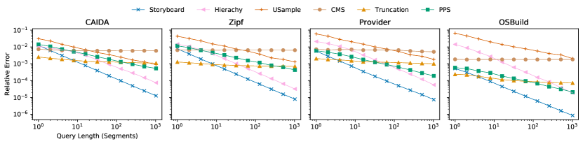
(a) Frequency Queries

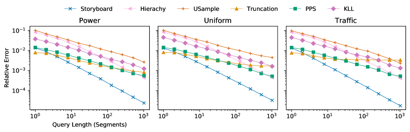
(b) Quantile Queries

Figure 5. Query error over interval queries of different lengths. Storyboard’s cooperative summaries have increasingly high accuracy as the query length increases.

6.2. Overall Query Accuracy

Summarization Methods. We compare a number of summarization techniques for frequencies and quantiles, and configure them to match total space usage when comparing accuracy. For all counter and sample-based summaries including CoopFreq, CoopQuant, and PPS, we set the number of counters or samples to the same $s$.

We compare against two popular mergeable summaries: the optimal quantiles sketch (KLL) from (Karnin et al., 2016), and the Count-Min frequency sketch (CMS) (Cormode and Muthukrishnan, 2005). For the count-min sketch we set $d=5$ and let the width $w=s$ parameter represent the space usage. We also compare against uniform random sampling (USample) (Cormode et al., 2012), and optimal single-segment summaries (Truncation) that summarize a segment by storing the exact item counts for the top $s$ items, or storing $s$ equally spaced values for quantiles.

For interval queries we also compare with storing Truncation summaries in a hierarchy (Hierarchy) following (Basat et al., 2018; Cormode et al., 2019). Specifically, the Hierarchy summarization strategy with base $b$ constructs $h$ layers of summaries. Summaries in layer $i$ are allocated space $b^{i}\cdot s_{0}$ to summarize aligned intervals of $b^{i}$ segments. Any query interval of length $k$ can be represented using $b\lceil{\log_{b}{k}}\rceil$ summaries from different layers. Since this requires maintaining $h=\log_{b}{k_{T}}$ layers, to fairly compare total space usage we scale the space $s_{0}$ allocated to the lowest layer summaries by a factor $s_{0}=s/\log_{b}{k_{T}}$. Unless otherwise stated we use $b=2$, though we will show in Section 6.3 that the choice does not have a significant impact on accuracy.

For cube queries we also compare with cube AQP techniques that use uniform USample with different space allocations: the USample:Prop method uses USample summaries but allocates space proportional to each segment size as a baseline random reservoir sample would (Vitter, 1985) while the STRAT method uses the method in the STRAT AQP system (Chaudhuri et al., 2007), which like Storyboard allocates space to minimize average error.

6.2.1. Interval Queries

We first evaluate Storyboard accuracy on interval queries, partitioning datasets with associated time or sequence columns into $k_{T}=2048$ size time segments. Then, we construct summaries with storage size $s=64$.

In Figures 5(a) and 5(b) we show how relative query error ${\epsilon^{\prime}}_{\mathcal{Q}}$ varies with the number of segments $k$ spanned by the interval. For $k=1,2,4,\dots,1024$ we sample 100 random start and end times for intervals with length $k$ and plot the average and standard deviation of the query error.

Storyboard, which uses cooperative summaries, outperforms any system that uses mergeable summaries or random sampling as $k$ increases. As the interval length increases merging the mergeable summaries (CMS, KLL) maintain their error as expected. Accumulating Truncation summaries also maintains the same constant error. Hierarchy, PPS, and USample are all able to reduce error when combining multiple summaries, while Cooperative summaries outperform all alternatives as $k$ exceeds 10 summaries. We also observe that despite our weaker worst-case bounds for cooperative quantile summaries, they achieve higher accuracy in practice compared to alternative methods. However, Storyboard gives up a constant factor in accuracy when aggregating less than $10$ summaries compared to alternatives.

6.2.2. Cube Queries

(a) Frequency Queries

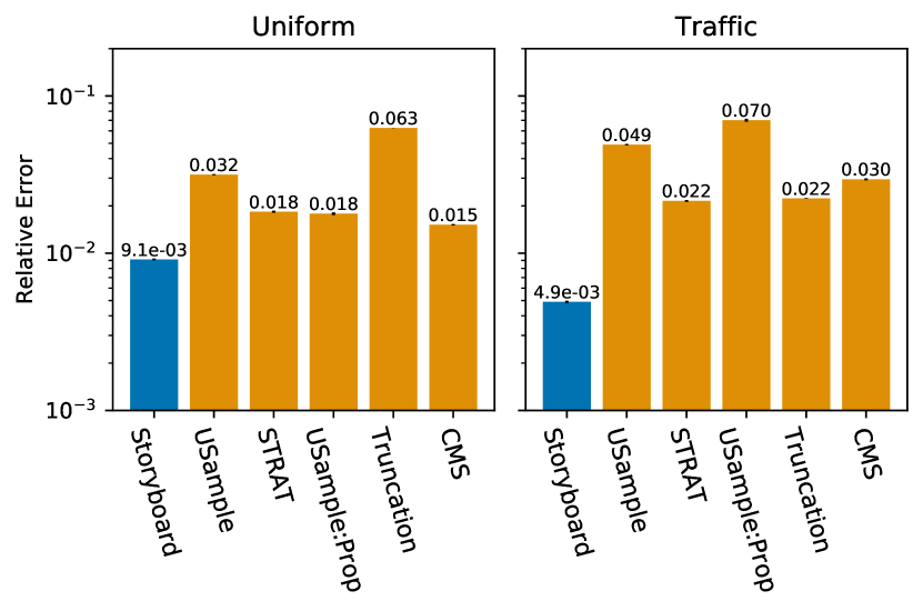
(b) Quantile Queries

Figure 6. Average query error over a workload of cube queries.

Table 2. Cube Datasets

Data	# Segments	Summary Space
Instacart	10080	300000
Zipf, Uniform	10000	50000
Traffic	4613	50000
OSBuild, Provider	4613	100000

We evaluate cube queries on our datasets with categorical dimension columns, and partitioned them along four dimension columns with parameters summarized in Table 2 and total space limit set to provide roughly consistent query error across the datasets. For each of these datasets we evaluate on a default query workload where each dimension has an independent $p=.2$ probability of being included as a filter, and if selected the dimension value is chosen uniformly at random.

In Figures 6(a) and 6(b) we show the average relative error for frequency and quantile queries over 10000 random cube queries drawn over the different dataset workloads. We see that, on average, Storyboard outperforms alternative summarization techniques that allocate equal space to each segment, as well as uniform sampling techniques that optimize sample size allocation.

6.3. Varying Parameters

Now we vary different system and summarization parameters to see their impact on accuracy, confirming that Storyboard is able to provide improved accuracy under a variety of conditions.

6.3.1. System Design

The Storyboard system depends on a number of parameters that go beyond a single summary. In this section we will show how accuracy varies with the accumulator size $s_{A}$, the size of cube aggregations, and the presence of each of the optimizations storyboard uses for data cubes.

Finite Accumulator.

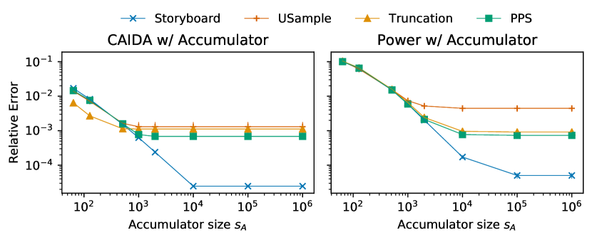
Figure 7. Query error as we vary the size of the accumulator $s_{A}$. For the large accumulators used in practice there is negligible additional error from the accumulator.

As described in Section 3.1, Storyboard accumulates precise frequency and ranks estimates from the summaries for point queries $\hat{g}(x)$, and accumulates summaries into a large accumulator $A$ for quantile and heavy hitters queries. In our evaluations thus far we have measured the maximum point query error, which bounds the maximum quantile or heavy hitter error as well (Section 3.4). The accumulator $A$ introduces an additional approximation error ${\epsilon^{\prime}}^{\text{(A)}}=1/s_{A}$ which is negligible as $s_{A}\rightarrow\infty$.

In Figure 7 we illustrate how using accumulators of different sizes, affects final query accuracy on the Power and CAIDA datasets. For each accumulator size, we measure the error after accumulating 100 random interval aggregations spanning $k=512$ segments. For the accumulators here we use SpaceSaving (Metwally et al., 2005) for frequency queries and a streaming implementation of PPS (VarOpt (Cohen et al., 2011)) for quantiles. ${\epsilon^{\prime}}^{\text{(A)}}$ quickly goes to $0$ as $s_{A}\rightarrow\infty$, so with at least 10 megabytes of memory available for $s_{A}$ the additional error is negligible.

Cube Query Spans. As seen already for interval queries, Storyboard improves the query error for queries combining results from multiple segment summaries. We can confirm this for cubes by looking at query error broken down by the number of dimensions in each query filter condition. Queries that filter on fewer columns will combine results from more segments. In Figure 8 we compare the error for queries that filter on different numbers of dimensions on the Uniform and Zipf cube workloads. Storyboard reduces the error for common queries that filter on zero or one dimension. As a tradeoff Storyboard incurs higher error than other methods for rarer queries with three or more filters. For a workload where queries with 3 or more filters are much less common than queries with 0 or 1 filters, this tradeoff is useful, and is configurable based on the user specified workload.

Cube Optimizer Lesion Study. In Figure 9 we show how the optimizations Storyboard (SB) uses for summarizing data cubes all play a role in providing high query accuracy by removing individual optimizations on the Zipf dataset. We experiment with removing the size optimizations (SB (-Size)) and bias optimizations (SB (-Bias)), and try replacing PPS summaries with uniform random samples (SB (-PPS)). When, size optimization or bias optimization are removed, error increases, and similarly error increases when PPS summaries are replaced with uniform random samples.

Cube Workload Specification. We also evaluate how Storyboard accuracy depends on precise workload specification by constructing Storyboard instances configured for incorrectly specified workloads. Rather than the true $p=0.2$ probability of including a dimension in the cube filter, we try optimizing cubes for $p=0.05$ in Work1 and $p=0.50$ in Work2. As included in Figure 9, in both cases error remains below existing cube construction methods. Interestingly, accuracy improves for Work1, indicating our optimization is not tight.

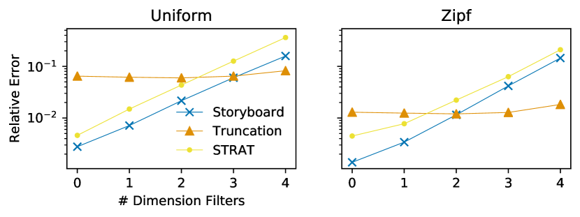
Figure 8. Query error broken down by number of dimension filters in a query. Storyboard achieves lower error on queries that have fewer filters and aggregate more segments.

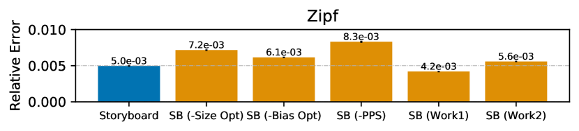
Figure 9. Lesion Study on Zipf cube optimizations. Removing any component reduces accuracy, though adjusting the workload parameter slightly improves accuracy.

Interval Length Specification. For interval aggregations users specify a maximum expected interval length $k_{T}$. In Figure 10 we show the relative error for 20 random queries of length $k=64$ as we vary $k_{T}$. All values $k_{T}\geq 64$ achieve good error and setting $k_{T}$ much larger does not negatively affect results. In practice accuracy is also robust to different values of $k_{T}$ as long as it is conservatively longer than the expected queries.

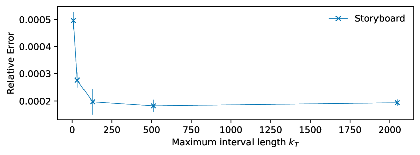
Figure 10. Error as we vary the maximum interval length parameter $k_{T}$. Overestimating $k_{T}$ does not significantly change the quality of results.

6.3.2. Summary Design

Now we will examine how Storyboard’s Cooperative and PPS summaries perform as individual segment summaries. The experiments below are run on the CAIDA dataset for interval aggregations.

Space Scaling. In Figure 11 we vary the space available to summaries for different interval lengths, confirming that like other state of the art summaries and sketches Cooperative and PPS summaries provide local segment error that scales inversely proportional to the space given, and maintain their accuracy under a wide range of summary sizes.

Hierarchical base $b$. Although Hierarchy summaries are parameterized by a base $b$, in Figure 12 we show that different values for $b$ do not noticeably improve performance. Although there are improvements in optimizing $b$ when merging small numbers ($k<10$) of summaries, the difference is less than $10\%$ for larger aggregations.

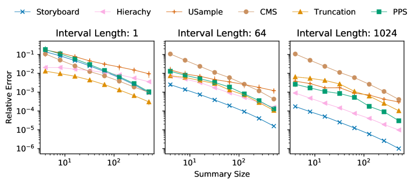
Figure 11. Query error as summary size changes. Cooperative summaries, like state of the art, have error ${\epsilon^{\prime}}=O(1/s)$

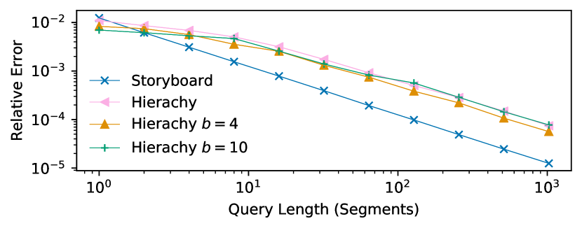
Figure 12. Hierarchy summary accuracy for different bases $b$. $b$ does not have a large impact when accumulating across multiple summaries.

.

7. Related Work

Precomputing Summaries. A number of existing approximate query processing (AQP) systems make use of precomputed approximate data summaries. An overview of these “offline” AQP systems can be found in (Li and Li, 2018), and they are an instance of the AggPre systems described in (Peng et al., 2018). Like data cube systems they materialize partial results (Harinarayan et al., 1996), but can support more complex query functions not captured by simple totals. Another class of systems use “online” AQP (Hellerstein et al., 1997; Budiu et al., 2019; Rabkin et al., 2014) and provide different latency and accuracy guarantees by computing approximations at query-time.

We are particularly motivated by Druid (Yang et al., 2014; Ray, 2013) and similar offline systems (Im et al., 2018) which aggregate over query-specific summaries for disjoint segments of data. However, these systems use mergeable summaries as-is, and do not optimize for improving accuracy under aggregation or take advantage of additional memory at query time to accumulate results more precisely. The authors in (Yi et al., 2014) apply hierarchical strategies to maintain summary collections for interval queries but like mergeable summaries maintain do not reduce error when combining summaries. Systems like BlinkDB (Agarwal et al., 2013), STRAT (Chaudhuri et al., 2007), and AQUA (Acharya et al., 1999) maintain random stratified samples to support general-purpose queries. Our choice of minimizing mean squared error over a workload follows the setup in STRAT (Chaudhuri et al., 2007). However, individual simple random samples are not as accurate as specialized frequency or quantile summaries (Mozafari and Niu, 2015).

Techniques for summarizing hierarchical intervals (Basat et al., 2018) are complementary, but incur additional storage overhead making them less accurate than Cooperative summaries and scale poorly to cubes with multiple dimensions (Qardaji et al., 2013).

Streaming and Mergeable Summaries. Many compact data summaries are developed in the streaming literature (Greenwald and Khanna, 2001; Misra and Gries, 1982; Cormode and Muthukrishnan, 2005; Karnin et al., 2016), including summaries for sliding windows (Arasu and Manku, 2004). However, they assume a different system model than Storyboard provides. The standard streaming model generally considers queries with working memory limited during summary construction (Muthukrishnan et al., 2005). Mergeable summaries (Agarwal et al., 2012) allow combining multiple summaries but require that intermediate results take up no more space than the inputs, and thus merely maintain relative error under merging. Other work targeting AggPre systems has focused on improving summary update and merge runtime performance (Gan et al., 2018; Masson et al., 2019) rather than improving the accuracy of merged summary results.

Other Summarization Models. The Storyboard model, where more memory is available for construction and aggregation than for storage, is closer to the model used in non-streaming settings including discrepancy theory and communication theory.

Coresets and $\epsilon$-approximations are data structures for approximate queries that allow more resource-intensive precomputation and aggregation (Phillips, 2017). $\epsilon$-approximations are part of discrepancy theory which attempts to approximate an underlying distribution with proxy samples (Chazelle, 2000). We draw inspiration from discrepancy theory to manage error accumulation in our cooperative summaries, especially the results in (Spencer, 1977) which pioneered the use of the $\cosh$ cost function. Other work in this area minimize error accumulation along multiple dimensions (Phillips, 2008). However, we are not away of coreset or $\epsilon$-approximations that allow for complex queries Storyboard supports: quantiles and item frequencies over multiple data segments. and cube aggregations. In particular, existing work supporting range queries (Phillips, 2008) do not provide per-segment local guarantees.

Work in communication theory and distributed streaming assume a setting where sending summaries over the network is a bottleneck equivalent to storage costs limits in Storyboard. There is existing work analyzing how multiple random samples can be combined to reduce aggregate error in this setting (Zengfeng Huang et al., 2011; Zhao et al., 2006). However, in communication theory the samples are constructed per-query, while Storyboard precomputes summaries that can be used for arbitrary future queries. Furthermore the random samples are not as space efficient as cooperative summaries.

Related techniques in differential privacy (Qardaji et al., 2013; Cormode et al., 2019) and matrix rounding (Doerr et al., 2006) consider approximate representations of data segments for the purposes of privacy, but do not explicitly optimize for space or support heavy hitters and quantile queries.

8. Conclusion

When aggregating multiple precomputed summaries, Storyboard optimizes and accumulates summaries for reduced query error. It does so by taking advantage of additional memory resources at summary construction and aggregation while targeting a common class of structured frequency and quantile queries. This system can thus efficiently serve a range of monitoring and data exploration workloads. Extensions to other query and aggregation types are a rich area for future work.

Appendix A Cooperative Summary Proofs

Lemma 1.

Proof.

Recall that we have a segment

$$\mathcal{D}_{t}=\{x_{1}\mapsto\delta_{1},\dots,x_{r}\mapsto\delta_{r}\}.$$

Let $H$ be the set of local heavy hitters $H=\{x_{i}:\delta_{i}\geq h\}$ and let $U^{\prime}=U\setminus H$ be the remaining items. We can decompose our summary as $S_{t}=S_{H}\cup S_{V}$ where $V=S_{t}\setminus H$.

(19) $$S_{H} =\{x_{i}\mapsto\delta_{i}:x_{i}\in H\}$$

(20) $$S_{V} =\{x_{i}\mapsto\min(\varepsilon_{t-1}(x_{i})+\delta_{i},rh):x_{i}\in V\}.$$

This keeps $\varepsilon_{t}(x)\geq 0$ across segments, i.e. our estimates are always underestimates.

Let $G=L_{t}-L_{t-1}=\sum_{x_{i}\in U}\left[\phi(\varepsilon_{t}(x_{i}))-\phi(\varepsilon_{t-1}(x_{i}))\right]$ where $\phi(z)=\exp(\alpha z)$. For heavy hitters $\varepsilon_{t}(x_{i})=\varepsilon_{t-1}(x_{i})$ so they do not change the cumulative cost $L_{t}$.

$$G =\sum_{x_{i}\in V}\left[\phi(\max(\varepsilon_{t-1}(x_{i})+\delta_{i}-rh,0))-\phi(\varepsilon_{t-1}(x_{i}))\right]$$

$$\quad+\sum_{x_{i}\in U^{\prime}\setminus V}\left[\phi(\varepsilon_{t-1}(x_{i})+\delta_{i})-\phi(\varepsilon_{t-1}(x_{i}))\right]$$

Simplifying using $\max(0,y)=y+(0-y)1_{y\leq 0}$ and $\phi(x+y)=\phi(x)\phi(y)$:

$$G =\sum_{x_{i}\in U^{\prime}\setminus V}\phi(\varepsilon_{t-1}(x_{i})+\delta_{i})\left[1-\phi(-\delta_{i})\right]$$

$$\quad+\sum_{x_{i}\in V}\phi(\varepsilon_{t-1}(x_{i})+\delta_{i})\left[\phi(-rh)-\phi(-\delta_{i})\right]$$

$$\quad+\sum_{x_{i}\in V}\left[\phi(0)-\phi(\varepsilon_{t-1}(x_{i})+\delta_{i}-rh)\right]\cdot 1_{\varepsilon_{t-1}+\delta_{i}\leq rh}$$

For non-heavy hitters, Algorithm 1 selects items in $V$ with the highest $\varepsilon_{t-1}(x_{i})+\delta_{i}$. If we let $\ell=\arg\min_{x_{i}\in V}\varepsilon_{t-1}(x_{i})+\delta_{i}$ then

$$\forall x_{i}\in V \quad\varepsilon_{t-1}(x_{\ell})+\delta_{\ell}\leq\varepsilon_{t-1}(x_{i})+\delta_{i}$$

$$\forall x_{i}\in U^{\prime}\setminus V \quad\varepsilon_{t-1}(x_{\ell})+\delta_{\ell}\geq\varepsilon_{t-1}(x_{i})+\delta_{i}.$$

Technical but standard applications of the inequalities $\phi(x)\geq 1+ax$, and $\phi(x)\leq 1+\alpha x+\alpha^{2}x^{2}/2$ for $x\leq 0$ yields:

$$G\leq \phi(\varepsilon_{t-1}(x_{\ell})+\delta_{\ell})|V|\left[\alpha h-\alpha hr+\alpha^{2}h^{2}r^{2}/2\right]+\alpha rh|V|$$

$|V|\leq s$ and $h\leq|\mathcal{D}_{t}|/s$ so when $\alpha\leq\frac{2}{h}\frac{r-1}{r^{2}}$, $G\leq\alpha r|\mathcal{D}_{t}|$ ∎

Lemma 3.

Proof.

First note that the choice of which element $z_{j}$ is chosen from each chunk for inclusion in the summary sample $S_{t}$ does not affect $\varepsilon_{t}(x)$ for $x$ outside the chunk $\mathcal{D}_{t,j}$ so we can consider the choices independently. This is because the selected element is assigned a proxy count equal to the population of the whole chunk $h=|\mathcal{D}_{t,j}|=|\mathcal{D}_{t}|/s$.

Let $L_{t,j}\coloneqq\sum_{x_{i}\in\mathcal{D}_{t,j}}\phi\left(\varepsilon_{t}(x_{i})\right)$ be total cost for chunk $j$. Since Algorithm 2 selects a value $z$ that minimizes $L_{t}$, the final value for $L_{t,j}$ must be lower than any weighted average of the possible $L_{t,j}$ for different choices of $x$.

$$L_{t,j} \leq\sum_{z\in\mathcal{D}_{t,j}}\frac{f_{\mathcal{D}_{t}}(z)}{h}\left[\sum_{x\in\mathcal{D}_{t,j}}\phi\left(\varepsilon_{t-1}(x)+r_{\mathcal{D}_{t,j}}(x)-1_{x\geq z}h\right)\right]$$

Abbreviate $p_{x}\coloneqq\frac{1}{h}r_{\mathcal{D}_{t,j}}(x)=\frac{1}{h}\sum_{x_{i}\in\mathcal{D}_{t,j}}\delta_{i}\cdot 1_{x_{i}\leq x}$. Switching the order of summation gives:

$$L_{t,j} \leq\sum_{x\in\mathcal{D}_{t,j}}[p_{x}\phi(\varepsilon_{t-1}(x)+hp_{x}-h)$$

$$\qquad+(1-p_{x})\phi(\varepsilon_{t-1}(x)+hp_{x})]$$

Now we can make use of Lemma 21 below to simplify

$$L_{t,j} \leq\exp(\alpha^{2}h^{2}/2)L_{t-1,j}$$

Finally, since $L_{t}=\sum_{j=1}^{s}L_{t,j}$ we have the lemma. ∎

Lemma 21 can be proven using the cosh angle addition formula and Taylor expansions.

Lemma 0.

For $0\leq p\leq 1$ and $t\geq 0$

(21) $$p\cosh(x+t(p-1))+(1-p)\cosh(x+tp)\leq\exp(t^{2}/2)\cosh(x)$$

Proof.

We abbreciate $\cosh,\sinh$ as $c,s$ and the left hand side of Equation 21 as $LHS$. Using the angle addition formula:

$$LHS =p\left[c(x)c(t(p-1))+s(x)s(t(p-1))\right]$$

$$\quad+(1-p)\left[c(x)c(tp)+s(x)s(tp)\right]$$

Then since $s(x)\leq c(x)$:

$$LHS \leq pc(x)\left[c(t(p-1))+s(t(p-1))\right]$$

$$\quad+(1-p)c(x)\left[c(tp)+s(tp)\right]$$

$$=c(s)\left[p\exp(t(p-1))+(1-p)\exp(tp)\right]$$

We now consider two cases: $t<2$ and $t\geq 2$.

If $t<2$, we expand out taylor series to get that:

$$p\exp(t(p-1))+(1-p)\exp(tp) \leq 1+\frac{t^{2}}{2}(p(1-p))\cdot 3$$

$$\leq 1+t^{2}/2\leq\exp(t^{2}/2)$$

If $t\geq 2$ then

$$p\exp(t(p-1))+(1-p)\exp(tp) \leq\exp(tp)$$

$$\leq\exp(t)\leq\exp(t^{2}/2)$$

In either case we can conclude that:

$$LHS \leq\cosh(x)\exp(t^{2}/2)$$

∎

A.1. Error Lower Bounds

In this section we will provide details on an adversarial dataset for which no online selection of items for a counter-based summary can achieve better than absolute $\varepsilon=\Omega(\log{k})$ error for item frequency queries.

Theorem 2.

There exists a sequence of $k=2^{h+1}$ data segments $\mathcal{D}_{i}$ consisting of $|\mathcal{D}_{i}|=2s$ item values each such that for all possible selections of $s$ items for counter-based summaries $S_{i}$, $\exists x.|f_{\mathcal{D}_{i},\dots,\mathcal{D}_{k}}(x)-\hat{f}_{S_{i},\dots,S_{k}}(x)|\geq h$.

Proof.

Consider a universe of item values $U=1,\dots,2s2^{h}$. For $i=1,\dots,2^{h}$ let $\mathcal{D}_{i}=\{2s(i-1)+1,\dots,2si\}$ where each item occurs at most once. Since each summary $S_{i}$ can only store $s$ item values, there must be a set of $s2^{h}$ items ($U_{1}$) that are not stored in any summary, but that have appeared at least once in the data. Now let the next $2^{h-1}$ data segments $\mathcal{D}_{i}$ for $i\geq 2^{h}+1$ constain $2s$ distinct item values each from $U_{1}$. Again, since each summary can only store $s$ item values now there must be a set of $s2^{h-1}$ items ($U_{2}$) that are not stored in any summary, but that have appeared twice in the data. This repeats for for increasing $U_{i}$: at each stage $U_{i}$ we have data segments come in that contain only items the summaries have not been able to store, until we have at least one item not stored in any summary but that has appeared $h+1$ times in the data. ∎

References

- (1)
- dru (2020) 2020. DataSketches Quantiles Sketch module. https://druid.apache.org/docs/latest/development/extensions-core/datasketches-quantiles.html.
- Abuzaid et al. (2018a) Firas Abuzaid, Peter Bailis, Jialin Ding, Edward Gan, Samuel Madden, Deepak Narayanan, Kexin Rong, and Sahaana Suri. 2018a. MacroBase: Prioritizing Attention in Fast Data. ACM Trans. Database Syst. 43, 4, Article 15 (2018), 45 pages.
- Abuzaid et al. (2018b) Firas Abuzaid, Peter Kraft, Sahaana Suri, Edward Gan, Eric Xu, Atul Shenoy, Asvin Ananthanarayan, John Sheu, Erik Meijer, Xi Wu, Jeff Naughton, Peter Bailis, and Matei Zaharia. 2018b. DIFF: A Relational Interface for Large-scale Data Explanation. PVLDB 12, 4 (2018), 419–432.
- Acharya et al. (1999) Swarup Acharya, Phillip B. Gibbons, Viswanath Poosala, and Sridhar Ramaswamy. 1999. The Aqua Approximate Query Answering System. In SIGMOD. 574–576.
- Agarwal et al. (2012) Pankaj K. Agarwal, Graham Cormode, Zengfeng Huang, Jeff Phillips, Zhewei Wei, and Ke Yi. 2012. Mergeable Summaries. In PODS.
- Agarwal et al. (2013) Sameer Agarwal, Barzan Mozafari, Aurojit Panda, Henry Milner, Samuel Madden, and Ion Stoica. 2013. BlinkDB: Queries with Bounded Errors and Bounded Response Times on Very Large Data. In EuroSys. 29–42.
- Arasu and Manku (2004) Arvind Arasu and Gurmeet Singh Manku. 2004. Approximate Counts and Quantiles over Sliding Windows. In PODS. 286–296.
- Basat et al. (2018) Ran Ben Basat, Roy Friedman, and Rana Shahout. 2018. Stream Frequency over Interval Queries. PVLDB 12, 4 (2018), 433–445.
- Budiu et al. (2019) Mihai Budiu, Parikshit Gopalan, Lalith Suresh, Udi Wieder, Han Kruiger, and Marcos K. Aguilera. 2019. Hillview: A Trillion-cell Spreadsheet for Big Data. PVLDB 12, 11 (July 2019), 1442–1457.
- Byrd et al. (1995) Richard H. Byrd, Peihuang Lu, Jorge Nocedal, and Ciyou Zhu. 1995. A Limited Memory Algorithm for Bound Constrained Optimization. SIAM J. Sci. Comput. 16, 5 (1995), 1190–1208.
- CAIDA (2016) CAIDA. 2016. The CAIDA UCSD Anonymized Internet Traces. http://www.caida.org/data/passive/passive_dataset.xml http://www.caida.org/data/passive/passive_dataset.xml.
- Chaudhuri et al. (2007) Surajit Chaudhuri, Gautam Das, and Vivek Narasayya. 2007. Optimized Stratified Sampling for Approximate Query Processing. ACM Trans. Database Syst. 32, 2 (2007).
- Chazelle (2000) Bernard Chazelle. 2000. The Discrepancy Method: Randomness and Complexity. Cambridge University Press, New York, NY, USA.
- Cohen et al. (2011) Edith Cohen, Graham Cormode, and Nick G. Duffield. 2011. Structure-Aware Sampling: Flexible and Accurate Summarization. PVLDB 4, 11 (2011), 819–830.
- Cormode et al. (2012) Graham Cormode, Minos Garofalakis, Peter J Haas, and Chris Jermaine. 2012. Synopses for massive data: Samples, histograms, wavelets, sketches. Foundations and Trends in Databases 4, 1–3 (2012), 1–294.
- Cormode and Hadjieleftheriou (2010) Graham Cormode and Marios Hadjieleftheriou. 2010. Methods for finding frequent items in data streams. The VLDB Journal 19, 1 (Feb 2010), 3–20.
- Cormode et al. (2019) Graham Cormode, Tejas Kulkarni, and Divesh Srivastava. 2019. Answering Range Queries Under Local Differential Privacy. PVLDB 12, 10 (2019), 1126–1138.
- Cormode and Muthukrishnan (2005) Graham Cormode and S. Muthukrishnan. 2005. An Improved Data Stream Summary: The Count-min Sketch and Its Applications. J. Algorithms 55, 1 (2005), 58–75.
- Doerr et al. (2006) Benjamin Doerr, Tobias Friedrich, Christian Klein, and Ralf Osbild. 2006. Unbiased Matrix Rounding. In Algorithm Theory – SWAT 2006, Lars Arge and Rusins Freivalds (Eds.). 102–112.
- Dua and Graff (2017) Dheeru Dua and Casey Graff. 2017. UCI Machine Learning Repository. http://archive.ics.uci.edu/ml
- Dunning and Ertl (2019) Ted Dunning and Otmar Ertl. 2019. Computing extremely accurate quantiles using t-digests. https://github.com/tdunning/t-digest. arXiv preprint arXiv:1902.04023 (2019).
- Gan et al. (2018) Edward Gan, Jialin Ding, Kai Sheng Tai, Vatsal Sharan, and Peter Bailis. 2018. Moment-based Quantile Sketches for Efficient High Cardinality Aggregation Queries. PVLDB 11, 11 (July 2018), 1647–1660.
- Gray et al. (1997) Jim Gray, Surajit Chaudhuri, Adam Bosworth, Andrew Layman, Don Reichart, Murali Venkatrao, Frank Pellow, and Hamid Pirahesh. 1997. Data cube: A relational aggregation operator generalizing group-by, cross-tab, and sub-totals. Data mining and knowledge discovery 1, 1 (1997), 29–53.
- Greenwald and Khanna (2001) Michael Greenwald and Sanjeev Khanna. 2001. Space-efficient online computation of quantile summaries. In SIGMOD, Vol. 30. 58–66.
- Harinarayan et al. (1996) Venky Harinarayan, Anand Rajaraman, and Jeffrey D. Ullman. 1996. Implementing Data Cubes Efficiently. In SIGMOD. 205–216.
- Hellerstein et al. (1997) Joseph M. Hellerstein, Peter J. Haas, and Helen J. Wang. 1997. Online Aggregation. In SIGMOD. 171–182.
- Ho et al. (1997) Ching-Tien Ho, Rakesh Agrawal, Nimrod Megiddo, and Ramakrishnan Srikant. 1997. Range Queries in OLAP Data Cubes. SIGMOD 26, 2 (1997), 73–88.
- Im et al. (2018) Jean-François Im, Kishore Gopalakrishna, Subbu Subramaniam, Mayank Shrivastava, Adwait Tumbde, Xiaotian Jiang, Jennifer Dai, Seunghyun Lee, Neha Pawar, Jialiang Li, and Ravi Aringunram. 2018. Pinot: Realtime OLAP for 530 Million Users. In SIGMOD. 583–594.
- Jones et al. (01 ) Eric Jones, Travis Oliphant, Pearu Peterson, et al. 2001–. SciPy: Open source scientific tools for Python. http://www.scipy.org/ [Online; accessed Oct 2019].
- Karnin et al. (2016) Z. Karnin, K. Lang, and E. Liberty. 2016. Optimal Quantile Approximation in Streams. In FOCS. 71–78.
- Li and Li (2018) Kaiyu Li and Guoliang Li. 2018. Approximate Query Processing: What is New and Where to Go? Data Science and Engineering 3, 4 (01 Dec 2018), 379–397.
- Luo et al. (2016) Ge Luo, Lu Wang, Ke Yi, and Graham Cormode. 2016. Quantiles over data streams: experimental comparisons, new analyses, and further improvements. VLDB 25, 4 (2016), 449–472.
- Masson et al. (2019) Charles Masson, Jee E. Rim, and Homin K. Lee. 2019. DDSketch: A Fast and Fully-Mergeable Quantile Sketch with Relative-Error Guarantees. PVLDB 12, 12 (Aug. 2019), 2195–2205.
- Metwally et al. (2005) Ahmed Metwally, Divyakant Agrawal, and Amr El Abbadi. 2005. Efficient Computation of Frequent and Top-k Elements in Data Streams. In Proceedings of the 10th International Conference on Database Theory (ICDT’05). 398–412.
- Misra and Gries (1982) J. Misra and David Gries. 1982. Finding repeated elements. Science of Computer Programming 2, 2 (1982), 143 – 152.
- Mozafari and Niu (2015) Barzan Mozafari and Ning Niu. 2015. A Handbook for Building an Approximate Query Engine. IEEE Data Eng. Bull. 38, 3 (2015), 3–29.
- Muthukrishnan et al. (2005) Shanmugavelayutham Muthukrishnan et al. 2005. Data streams: Algorithms and applications. Foundations and Trends® in Theoretical Computer Science 1, 2 (2005), 117–236.
- Peng et al. (2018) Jinglin Peng, Dongxiang Zhang, Jiannan Wang, and Jian Pei. 2018. AQP++: Connecting Approximate Query Processing With Aggregate Precomputation for Interactive Analytics. In SIGMOD. 1477–1492.
- Phillips (2008) Jeff M. Phillips. 2008. Algorithms for -Approximations of Terrains. In Proceedings of the 35th International Colloquium on Automata, Languages and Programming - Volume Part I (ICALP ’08). 447–458.
- Phillips (2017) Jeff M. Phillips. 2017. Coresets and Sketches. In Handbook of Discrete and Computational Geometry, Csaba D. Toth, Joseph O’Rourke, and Jacob E. Goodman (Eds.). CRC Press, Chapter 48, 1267–1286.
- Qardaji et al. (2013) Wahbeh Qardaji, Weining Yang, and Ninghui Li. 2013. Understanding Hierarchical Methods for Differentially Private Histograms. PVLDB 6, 14 (Sept. 2013), 1954–1965.
- Rabkin et al. (2014) Ariel Rabkin, Matvey Arye, Siddhartha Sen, Vivek S. Pai, and Michael J. Freedman. 2014. Aggregation and Degradation in JetStream: Streaming Analytics in the Wide Area. In NSDI. 275–288.
- Ray (2013) Nelson Ray. 2013. The Art of Approximating Distributions: Histograms and Quantiles at Scale. http://druid.io/blog/2013/09/12/the-art-of-approximating-distributions.html.
- Spencer (1977) Joel Spencer. 1977. Balancing games. Journal of Combinatorial Theory, Series B 23, 1 (1977), 68 – 74.
- Ting (2018) Daniel Ting. 2018. Data Sketches for Disaggregated Subset Sum and Frequent Item Estimation. In SIGMOD. 1129–1140.
- Vitter (1985) Jeffrey S. Vitter. 1985. Random Sampling with a Reservoir. ACM Trans. Math. Softw. 11, 1 (1985), 37–57.
- Yang et al. (2014) Fangjin Yang, Eric Tschetter, Xavier Léauté, Nelson Ray, Gian Merlino, and Deep Ganguli. 2014. Druid: A Real-time Analytical Data Store. In SIGMOD. 157–168.
- Yi et al. (2014) Ke Yi, Lu Wang, and Zhewei Wei. 2014. Indexing for Summary Queries: Theory and Practice. ACM Trans. Database Syst. 39, 1 (Jan. 2014).
- Zengfeng Huang et al. (2011) Zengfeng Huang, Ke Yi, Yunhao Liu, and Guihai Chen. 2011. Optimal sampling algorithms for frequency estimation in distributed data. In 2011 Proceedings IEEE INFOCOM. 1997–2005.
- Zhao et al. (2006) Qi (George) Zhao, Mitsunori Ogihara, Haixun Wang, and Jun (Jim) Xu. 2006. Finding Global Icebergs over Distributed Data Sets. In PODS. 298–307.