Snippext: Semi-supervised Opinion Mining with Augmented Data

Abstract.

Online services are interested in solutions to opinion mining, which is the problem of extracting aspects, opinions, and sentiments from text. One method to mine opinions is to leverage the recent success of pre-trained language models which can be fine-tuned to obtain high-quality extractions from reviews. However, fine-tuning language models still requires a non-trivial amount of training data.

In this paper, we study the problem of how to significantly reduce the amount of labeled training data required in fine-tuning language models for opinion mining. We describe $\mathsf{Snippext}$, an opinion mining system developed over a language model that is fine-tuned through semi-supervised learning with augmented data. A novelty of $\mathsf{Snippext}$ is its clever use of a two-prong approach to achieve state-of-the-art (SOTA) performance with little labeled training data through: (1) data augmentation to automatically generate more labeled training data from existing ones, and (2) a semi-supervised learning technique to leverage the massive amount of unlabeled data in addition to the (limited amount of) labeled data. We show with extensive experiments that $\mathsf{Snippext}$ performs comparably and can even exceed previous SOTA results on several opinion mining tasks with only half the training data required. Furthermore, it achieves new SOTA results when all training data are leveraged. By comparison to a baseline pipeline, we found that $\mathsf{Snippext}$ extracts significantly more fine-grained opinions which enable new opportunities of downstream applications.

1. Introduction

Online services such as Amazon, Yelp, or Booking.com are constantly extracting aspects, opinions, and sentiments from reviews and other online sources of user-generated information. Such extractions are useful for obtaining insights about services, consumers, or products and answering consumer questions. Aggregating the extractions can also provide summaries of actual user experiences directly to consumers so that they do not have to peruse all reviews or other sources of information. One method to easily mine opinions with a good degree of accuracy is to leverage the success of pre-trained language models such as BERT (Devlin et al., 2018) or XLNet (Yang et al., 2019) which can be fine-tuned to obtain high-quality extractions from text. However, fine-tuning language models still requires a significant amount of high-quality labeled training data. Such labeled training data are usually expensive and time-consuming to obtain as they often involve a great amount of human effort. Hence, there has been significant research interest in obtaining quality labeled data in a less expensive or more efficient way (Settles et al., 2008; Settles, 2009).

In this paper, we study the problem of how to reduce the amount of labeled training data required in fine-tuning language models for opinion mining. We describe $\mathsf{Snippext}$, an opinion mining system developed based on a language model that is fine-tuned through semi-supervised learning with augmented data. $\mathsf{Snippext}$ is motivated by the need to accurately mine opinions, with small amounts of labeled training data, from reviews of different domains, such as hotels, restaurants, companies, etc.

Example 1.1.

$\mathsf{Snippext}$ mines three main types of information from reviews: aspects, opinions, and sentiments, which the following example illustrates.

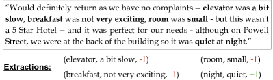
Figure 1. Extractions from a hotel review.

Figure 1 shows an example where triples of the form $(\mathsf{asp},\mathsf{opi},s)$ are derived from a hotel review. For example, the triple (elevator, a bit slow, -1) consists of two spans of tokens that are extracted from the review, where “a bit slow” is an opinion term about the aspect term “elevator”. The polarity score -1 is derived based on the sentence that contains the aspect and opinion terms and it indicates a negative sentiment in this example. (1 indicates positive, -1 is negative, and 0 is neutral.)

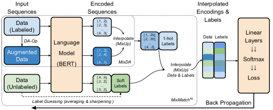
Figure 2. Overall Architecture of $\mathsf{Snippext}$. $\mathsf{MixDA}$ augments and interpolate the labeled training sequences. $\mathsf{MixMatch^{NL}}$ further combines labeled and unlabeled data into supervisory signal for fine-tuning the pre-trained Language Model (LM).

As mentioned earlier, one can simply fine-tune a pre-trained language model such as BERT (Devlin et al., 2018) using labeled training data to obtain the triples as shown in Figure 1. Recent results (Xu et al., 2019; Sun et al., 2019a; Li et al., 2019) showed that BERT with fine-tuning achieved state-of-the-art (SOTA) performance in many extraction tasks, outperforming previous customized neural network approaches. However, the fine-tuning approach still requires a significant amount of high-quality labeled training data. For example, the SOTA for aspect term extraction for restaurants is trained on 3,841 sentences labeled by linguistic experts through a non-trivial process (Pontiki et al., 2014). In many cases, labeled training data are obtained by crowdsourcing (Li et al., 2016). Even if the monetary cost of crowdsourcing may not be an issue, preparing crowdsourcing task, launching, and post-processing the results are usually very time-consuming. The process often needs to be repeated a few times to make necessary adjustments. Also, in many cases, measures have to be taken to remove malicious crowdworkers and to ensure the quality of crowdworkers. Furthermore, the labels for a sentence have to be collected several times to reduce possible errors and the results have to be cleaned before they are consumable for downstream tasks. Even worse, this expensive labeling process has to be repeated to train the model on each different domain (e.g., company reviews).

Motivated by the aforementioned issues, we investigate the problem of reducing the amount of labeled training data required for fine-tuning language models such as BERT. Specifically, we investigate solutions to the following problem.

Problem 1.

Given the problem of extracting aspect and opinion pairs from reviews, and deriving the corresponding sentiment of each aspect-opinion pair, can we fine-tune a language model with half (or less) of training examples and still perform comparably with the SOTA?

Contributions  We present $\mathsf{Snippext}$, our solution to the above problem. The architecture of $\mathsf{Snippext}$ is depicted in Figure 2. Specifically, we make the following contributions:

• We developed $\mathsf{Snippext}$ (snippets of extractions), a system for extracting aspect and opinion pairs, and corresponding sentiments from reviews by fine-tuning a language model with very little labeled training data. $\mathsf{Snippext}$ is not tied to any language model although we use the state-of-the-art language model BERT for our implementation and experiments as depicted in Figure 2.

• A novelty of $\mathsf{Snippext}$ is the clever use of a two-prong approach to achieve SOTA performance with little labeled training data: through (1) data augmentation to automatically generate more labeled training data ($\mathsf{MixDA}$, top-left of Figure 2), and through (2) a semi-supervised learning technique to leverage the massive amount of unlabeled data in addition to the (limited amount of) labeled data ($\mathsf{MixMatch^{NL}}$, right half of Figure 2). The unlabeled data allows the trained model to better generalize the entire data distribution and avoid overfitting to the small training set.

• $\mathsf{Snippext}$ introduces a new data augmentation technique, called $\mathsf{MixDA}$, which allows one to only “partially” transform a text sequence so that the resulting sequence is less likely to be distorted. This is done by a non-trivial adaptation of the $\mathsf{MixUp}$ technique, which we call $\mathsf{MixUp^{NL}}$, from computer vision to text (see Section 3). $\mathsf{MixUp^{NL}}$ uses the convex interpolation technique on the text’s language model encoding rather than the original data. With $\mathsf{MixDA}$, we develop a set of effective data augmentation ($\mathsf{DA}$) operators suitable for opinion mining tasks.

• $\mathsf{Snippext}$ exploits the availability of unlabeled data through a component called $\mathsf{MixMatch^{NL}}$, which is a novel adaptation of $\mathsf{MixMatch}$ (Berthelot et al., 2019b) from images to text. $\mathsf{MixMatch^{NL}}$ guesses the labels for unlabeled data and interpolates data with guessed labels and data with known labels. While the guess and interpolate idea has been carried out in computer vision for training high-accuracy image classifiers, this is the first time the idea is adapted for text. $\mathsf{MixMatch^{NL}}$ leverages $\mathsf{MixUp^{NL}}$(described earlier). Our data augmentation based on $\mathsf{MixDA}$ also provides further performance improvement to $\mathsf{MixMatch^{NL}}$.

• We evaluated the performance of $\mathsf{Snippext}$ on four Aspect-Based Sentiment Analysis (ABSA) benchmark datasets. The highlights of our experimental analysis include: (1) We achieve new SOTA F1/Macro-F1 scores on all four tasks established by $\mathsf{MixDA}$ and $\mathsf{MixMatch^{NL}}$ of $\mathsf{Snippext}$. (2) Further, a surprising result is that we already achieve the previous SOTA when given only 1/2 or even 1/3 of the original training data.

• We also evaluate the practical impact of $\mathsf{Snippext}$ by applying it to a large real-world hotel review corpus. Our analysis shows that $\mathsf{Snippext}$ is able to extract more fine-grained opinions/customer experiences that are missed by previous methods.

Outline  In Section 2, we overview $\mathsf{Snippext}$ and its core modules. We introduce our data augmentation technique $\mathsf{MixDA}$ in Section 3. Section 4 introduces $\mathsf{MixMatch^{NL}}$, an adaptation of $\mathsf{MixMatch}$ to text. We show our experiment results in Section 5 and 6. Finally, we discuss related work in Sections 7 and conclude in Section 8.

2. Preliminary

Table 1. Different tasks in ABSA and $\mathsf{Snippext}$.

Tasks	Task Types	Vocabulary	Examples Input/Output
Aspect/Opinion Ext. (similarly for AE in ABSA)	Tagging	{B-AS, I-AS, B-OP, I-OP, O}	$S=$ Everybody was very nice , but the food was average at best . $\Rightarrow$ B-AS O B-OP I-OP O O O B-AS O B-OP I-OP I-OP O
Aspect Sentiment Cls.	Span Cls.	{-1, +1, 0}	$P=\{(1,1)\}$ (i.e.,“Everybody”) $\Rightarrow+1$ ; $P=\{(8,8)\}$ (i.e.,“food”) $\Rightarrow 0$
Attribute Cls.	Span Cls.	Domain-specific attributes	$P=\{(1,1)\}$ $\Rightarrow\mathbf{Staff}$ ; $P=\{(8,8)\}$ $\Rightarrow\mathbf{Food}$
Aspect/Opinion Pairing	Span Cls.	{PAIR, NOTPAIR}	$P=\{(1,1),(3,4)\}\Rightarrow$ PAIR ; $P=\{(8,8),(3,4)\}\Rightarrow$ NOTPAIR ($\times$“very nice food”)

The goal of $\mathsf{Snippext}$ is to extract high-quality information from text with small amounts of labeled training data. In this paper, we focus on four main types of extraction tasks, which can be formalized as either tagging or span classification problems.

2.1. Tagging and Span Classification

Types of extraction tasks  Figure 1 already illustrates the tagging and sentiment classification extraction tasks. Implicit in Figure 1 is also the pairing task that understands which aspect and opinion terms go together. Figure 3 makes these tasks explicit, where in addition to tagging, pairing, and sentiment classification, there is also the attribute classification task, which determines which attribute a pair of aspect and opinion terms belong to. Attributes are important for downstream applications such as summarization and query processing (Li et al., 2019; Evensen et al., 2019). As we will describe, sentiment classification, pairing, and attribute classification are all instances of the span classification problem. In what follows, we sometimes refer to an aspect-opinion pair as an opinion.

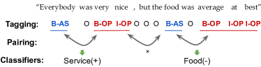
Figure 3. The tagging model identifies all aspect (AS) and opinion (OP) spans. Among all candidate pairs of AS-OP spans, the pairing model identifies the correct associations, e.g., (“very nice”, “Everybody”) is correct but not (“very nice”, “food”). Finally, there are two classifiers decide: (1) which attribute that an extracted pair should be assigned to and (2) the sentiment (positive, negative, or neutral) of the opinion.

Definition 2.1.

(Tagging) Let $V$ be a vocabulary of labels. A tagging model $M$ takes as input a sequence $S=[s_{1},\dots,s_{n}]$ of tokens and outputs a sequence of labels $M(S)=[l_{1},\dots,l_{n}]$ where each label $l_{i}\in V$.

Aspect and opinion term extractions are sequence tagging tasks as in ABSA  (Wang et al., 2016, 2017; Li et al., 2019; Xu et al., 2019), where $V=\{\mathsf{B\text{-}AS},\mathsf{I\text{-}AS},\mathsf{B\text{-}OP},\mathsf{I\text{-}OP},\\ \mathsf{O}\}$ using the classic IOB format. The $\mathsf{B\text{-}AS}$/$\mathsf{B\text{-}OP}$ tags indicate that a token is at the beginning of an aspect/opinion term, the $\mathsf{I\text{-}AS}$/$\mathsf{I\text{-}OP}$ tags indicate that a token is inside an aspect/opinion term and $\mathsf{O}$ tags indicate that a token is outside of any aspect/opinion term.

Definition 2.2.

(Span Classification) Let $V$ be a vocabulary of class labels. A span classifier $M$ takes as input a sequence $S=[s_{1},\dots,s_{n}]$ and a set $P$ of spans. Each span $p\in P$ is represented by a pair of indices $p=(a,b)$ where $1\leq a\leq b\leq n$ indicating the start/end positions of the span. The classifier outputs a class label $M(S,P)\in V$.

Both Aspect Sentiment Classification (ASC) (Xu et al., 2019; Sun et al., 2019a) and the aspect-opinion pairing task can be formulated as span classification tasks (Li et al., 2019). For ASC, the span set $P$ contains a single span which is the targeted aspect term. The vocabulary $V=\{+1,0,-1\}$ indicates positive, neutral, or negative sentiments. For pairing, $P$ contains two spans: an aspect term and an opinion term. The vocabulary $V=\{\mathsf{PAIR},\mathsf{NOTPAIR}\}$ indicates whether the two spans in $P$ are correct pairs to be extracted or not. Attribute classification can be captured similarly. Table 1 summarizes the set of tasks considered in ABSA and $\mathsf{Snippext}$.

2.2. Fine-tuning Pre-trained Language Models

Figure 2 shows the basic model architecture in $\mathsf{Snippext}$, where it makes use of a pre-trained language model (LM).

Pre-trained LMs such as BERT (Devlin et al., 2018), GPT-2 (Radford et al., 2018), and XLNet (Yang et al., 2019) have demonstrated good performance in a wide range of NLP tasks. In our implementation, we use the popular BERT language model although our proposed techniques (detailed in Sections 3 and 4) are independent of the choice of LMs. We optimize BERT by first fine-tuning it with a domain-specific text corpus then fine-tune the resulting model for the different subtasks. This has been shown to be a strong baseline for various NLP tasks (Beltagy et al., 2019; Lee et al., 2019; Xu et al., 2019) including ABSA.

Fine-tuning LMs for specific subtasks. Pre-trained LMs can be fine-tuned to a specific task through a task-specific labeled training set as follows:

1. Add task-specific layers (e.g., a simple fully connected layer for classification) after the final layer of the LM;

2. Initialize the modified network with parameters from the pre-trained model;

3. Train the modified network on the task-specific labeled data.

We fine-tune BERT to obtain our tagging and span classification models. For both tagging and span classification, the task-specific layers consist of only one fully connected layer followed by a softmax output layer. The training data also need to be encoded into BERT’s input format. We largely follow the fine-tuning approach described in (Devlin et al., 2018; Xu et al., 2019) and Figure 4 shows an example of the model architecture for tagging aspect/opinion terms. We describe more details in Section 5.

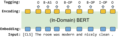
Figure 4. Fine-tuning BERT for aspect/opinion term extraction.

As mentioned earlier, our proposed techniques are independent of the choice of LMs and task-specific layers. We use the basic 12-layer uncased BERT and one fully connected task-specific layer in this paper but one can also use higher-quality models with deeper LMs (e.g., a larger BERT or XLNet) or adopt more complex task-specific layers (e.g., LSTM and CRF) to further improve the results obtained.

Challenges in optimizing LMs. It has been shown that fine-tuning BERT for specific tasks achieves good results, often outperforming previous neural network models for multiple tasks of our interest (Xu et al., 2019; Sun et al., 2019b). However, like in many other deep learning approaches, to achieve good results on fine-tuning for specific tasks requires a fair amount of quality labeled training data (e.g., 3,841 labeled sentences were used for aspect term extraction for restaurants (Pontiki et al., 2014, 2015)) and creating such datasets with desired quality is often expensive.

$\mathsf{Snippext}$ overcomes the requirement of having a large quality labeled training set by addressing the following two questions:

• Can we make the best of a small set of labeled training data by generating high-quality training examples from it?

• Can we leverage BOTH labeled and unlabeled data for fine-tuning the in-domain LM for specific tasks and obtain better results?

We address these two questions in Sections 3 and 4 respectively.

3. MixDA: augment and interpolate

Data augmentation ($\mathsf{DA}$) is a technique to automatically increase the size of the training data without using human annotators. DA is shown to be effective for certain tasks in computer vision and NLP. In computer vision, labeled images that are augmented through simple operators such as rotate, crop, pad, flip are shown to be effective for training deep neural networks (Perez and Wang, 2017; Cubuk et al., 2018). In NLP, sentences that are augmented by replacing tokens with their corresponding synonyms are shown to be effective for training sentence classifiers (Wei and Zou, 2019). Intuitively, such augmented data allow the trained model to learn properties that remain invariant in the data (e.g., the meaning of a sentence remains unchanged if a token is replaced with its synonym). However, in NLP tasks the use of DA is still limited, as synonyms of a word are very limited and other operators can distort the meaning of the augmented sentence. Motivated by above issues and inspired by the ideas of data augmentation and $\mathsf{MixUp}$ (Zhang et al., 2017), we introduce the $\mathsf{MixDA}$ technique that generates augmented data through (1) carefully augmenting the set of labeled sentences through a set of data augmentation operators suitable for tagging and span-classification, and (2) performing a convex interpolation on the augmented data with the original data to further reduce the noise that may occur in the augmented data. $\mathsf{MixDA}$ uses the resulting interpolation as the training signal.

3.1. Data Augmentation Operators

The typical data augmentation operators that have been proposed for text (Wei and Zou, 2019; Xie et al., 2019) include: token replacement (replaces a token with a new one in the example); token insertion (inserts a token into the example); token deletion (removes a token from the example); token swap (swaps two tokens in the example); and back translation (translates the example into a different language and back, e.g., EN $\rightarrow$ FR $\rightarrow$ EN).

Although these operators were shown to be effective in augmenting training data for sentence classification, a naive application of these operators can be problematic for the tagging or span classification tasks as the following example illustrates.

The	food	was	average	at	best	.
O	B-AS	O	B-OP	I-OP	I-OP	O

A naive application of swap or delete may leave the sequence with an inconsistent state of tags (e.g., if “average” was removed, I-OP is no longer preceded by B-OP). Even worse, replace or insert can change the meaning of tokens and also make the original tags invalid (e.g., by replacing “at” with “and”, the correct tags should be “average (B-OP) and(O) best(B-OP)”). Additionally, back translation changes the sentence structure and tags are lost during the translation.

The above example suggests that $\mathsf{DA}$ operators must be carefully applied. Towards this, we distinguish two types of tokens. We call the consecutive tokens with non-“$\mathsf{O}$” tags (or consecutive tokens represented by a pair of indices in span classification tasks), the target spans. The tokens within target spans are target tokens and the tokens with “$\mathsf{O}$” tags, are the non-target tokens. To guarantee the correctness of the tagging sequence, we apply $\mathsf{DA}$ operators over target spans and non-target tokens. Specifically, we consider only 4 token-level operators similar to what was described earlier (TR (replace), INS (insert), DEL (delete), and SW (swap)) but apply them only on non-target tokens. We also introduced a new span-level operator (SPR for span-level replacement), which augments the input sequences by replacing a target span with a new span of the same type. Table 2 summarizes the set of $\mathsf{DA}$ operators in $\mathsf{Snippext}$.

Table 2. $\mathsf{DA}$ operators of $\mathsf{Snippext}$. TR, INS, DEL, SW are modified from prior operators. SPR is a new span-level operator.

Operator	Description
TR	Replace non-target token with a new token.
INS	Insert before or after a non-target token with a new token.
DEL	Delete a non-target token.
SW	Swap two non-target tokens.
SPR	Replace a target span with a new span.

To apply a $\mathsf{DA}$ operator, we first sample a token (or span) from the original example. If the operator is INS, TR, or SPR, then we also need to perform a post-sampling step to determine a new token (or span) to insert or replace the original one. There are two strategies for sampling (and one more for post sampling):

• Uniform sampling: picks a token or span from the sequence with equal probability. This is a commonly used strategy as in (Wei and Zou, 2019).

• Importance-based sampling: picks a token or span based on probability proportional to the importance of the token/span, which is measured by the token’s TF-IDF (Xie et al., 2019) or the span’s frequency.

• Semantic Similarity (post-sampling only): picks a token or span with probability proportional to its semantic similarity with the original token/span. Here, we measure the semantic similarity by the cosine similarity over token’s or span’s embeddings.

For INS/TR/SPR, the post-sampling step will pick a similar token (resp. span) to insert or to replace the token (resp. span) that was picked in the pre-sampling step. We explored different combinations of pre-sampling and post-sampling strategies and report the most effective strategies in Section 5.

3.2. Interpolate

Although the $\mathsf{DA}$ operators are designed to minimize distortion to the original sentence and its labels, the operators can still generate examples that are “wrong” with regard to certain labels. As we found in Section 5.3, these wrong labels can make the $\mathsf{DA}$ operator less effective or even hurt the resulting model’s performance.

Example 3.1.

Suppose the task is to classify the aspect sentiment of “Everybody”:

Everybody (+1) was very nice …

The $\mathsf{DA}$ operators can still generate examples that are wrong with regard to the labels. For example, TR may replace “nice” with a negative/neutral word (e.g., “poor”, “okay”) and hence the sentiment label is no longer +1. Similarly, DEL may drop “nice”, INS may insert “sometimes” after “was”, or SPR can replace “Everybody” with “Nobody” so that the sentiment label would now be wrong.

To reduce the noise that may be introduced by the augmented data, we propose a novel technique called $\mathsf{MixDA}$ that performs a convex interpolation on the augmented data with the original data and uses the interpolated data as training data instead. Intuitively, the interpolated result is an intermediary between an example and an augmented example. By taking this “mixed” example, which is only“partially augmented” and “closer” to the original example than the augmented example, the resulting training data are likely to contain less distortion.

MixUp^NL. Let $x_{1}$ and $x_{2}$ be two text sequences and $y_{1}$ and $y_{2}$ as their one-hot label vectors respectively. We assume that both sequences are padded into the same length. We first create two new sequences $x^{\prime}$ and $y^{\prime}$ as follows:

(1) $$\mathsf{BERT}(x^{\prime}) = \lambda\cdot\mathsf{BERT}(x_{1})+(1-\lambda)\cdot\mathsf{BERT}(x_{2})$$

(2) $$y^{\prime} = \lambda\cdot y_{1}+(1-\lambda)\cdot y_{2}\vspace{-1mm}$$

where $\mathsf{BERT}(x_{1})$ and $\mathsf{BERT}(x_{2})$ are the BERT encoding for $x_{1}$ and $x_{2}$, $y_{1}$ are original labels of $x_{1}$, $y_{2}$ labels are generated directly from $y_{1}$ when performing DA operators, and $\lambda\in[0,1]$ is a random variable sampled from a symmetric Beta distribution $\text{Beta}(\alpha,\alpha)$ for a hyper-parameter $\alpha$. Note that we do not actually generate the interpolated sequence $x^{\prime}$ but instead, only use the interpolated encoding $\mathsf{BERT}(x^{\prime})$ to carry out the computation in the task-specific layers of the neural network. Recall that the task-specific layers for tagging take as input the entire $\mathsf{BERT}(x^{\prime})$ while the span-classification tasks only require the encoding of the aggregated “$\mathsf{[CLS]}$” token.

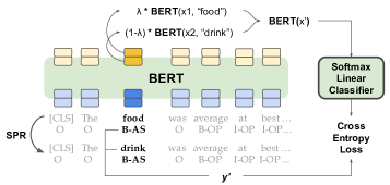
Figure 5. MixDA augments by interpolating over the BERT encoding.

Figure 5 illustrates how we train a model using the results of $\mathsf{MixDA}$. Given an example $(x,y)$, $\mathsf{MixDA}$ trains a model through three main steps:

• Data Augmentation: a $\mathsf{DA}$ operator (see Section 3.1) is applied to obtain $(x_{\text{aug}},y_{\text{aug}})$.

• Interpolation: perform the $\mathsf{MixUp^{NL}}$ interpolation on the pair of input $(x,y)$ and $(x_{\text{aug}},y_{\text{aug}})$ to obtain $(\mathsf{BERT}(x^{\prime}),y^{\prime})$. The resulting $\mathsf{BERT}(x^{\prime})$ corresponds to the encoding of a sequence “in between” the original sequence $x$ and the fully augmented sequence $x_{\text{aug}}$.

• Back Propagation: feed the interpolated encoding $\mathsf{BERT}(x^{\prime})$ to the remaining layers, compute the loss over $y^{\prime}$, and back propagate to update the model.

• Data Augmentation Optimization: Since $\mathsf{DA}$ operators may change the sequence length, for tagging, $\mathsf{MixDA}$ also carefully aligns the label sequence $y_{\text{aug}}$ with $y$. This is done by padding tokens to both $x$ and $x_{\text{aug}}$ when the inserting/deleting/replacing of tokens/spans creates misalignments in the two sequences. When the two sequences are perfectly aligned, Equation 2 simplifies to $y^{\prime}=y_{1}$.

Intuitively, by the interpolation, $\mathsf{MixDA}$ allows an input sequence to be augmented by a $\mathsf{DA}$ operator partially (by a fraction of $1-\lambda$) to effectively reduce the distortion produced by the original operator. Our experiment results in Section 5.3 confirms that applying $\mathsf{DA}$ operators with $\mathsf{MixDA}$ is almost always beneficial (in 34/36 cases) and can result in up to 2% performance improvement in aspect sentiment classification.

Discussion. The interpolation step of $\mathsf{MixDA}$ is largely inspired by the $\mathsf{MixUp}$ operator (Zhang et al., 2017; Verma et al., 2018) in computer vision, which has been shown to be a very effective regularization technique for learning better image representations. $\mathsf{MixUp}$ produces new training examples by combining two existing examples through their convex interpolation. With the interpolated examples as training data, the trained model can now make predictions that are “smooth” in between the two examples. For example, in a binary classification of cat and dog images, the model would learn that (1) the “combination” of two cats (or dogs) should be classified as cat (or dog); (2) something “in between” a cat and a dog should be given less confidence, i.e., the model should predict both classes with similar probability.

Unlike images, however, text sequences are not continuous and have different lengths. Thus, we cannot apply convex interpolation directly over the sequences. In $\mathsf{Snippext}$, we compute the language model’s encoding of the two sequences and interpolate the encoded sequences instead. A similar idea was considered in computer vision (Verma et al., 2018) and was shown to be more effective than directly interpolating the inputs. Furthermore, in contrast to image transformations that generate a continuous range of training examples in the vicinity of the original image, traditional text $\mathsf{DA}$ operators only generate a limited finite set of examples. $\mathsf{MixDA}$ increases the coverage of $\mathsf{DA}$ operators by generating varying degrees of partially augmented training examples. Note that $\mathsf{MixUp}$ has been applied in NLP in a setting (Guo et al., 2019) with sentence classification and CNN/RNN-based models. To the best of our knowledge, $\mathsf{MixDA}$ is the first to apply $\mathsf{MixUp}$ on text with a pre-trained LM and data augmentation.

4. Semi-Supervised Learning with MixMatch^NL

Semi-supervised learning (SSL) is the learning paradigm (Zhu, 2005) where models learn from a small amount of labeled data and a large amount of unlabeled data. We propose $\mathsf{MixMatch^{NL}}$, a novel SSL framework for NLP based on an adaptation of $\mathsf{MixMatch}$ (Berthelot et al., 2019b), which is a recently proposed technique in computer vision for training high-accuracy image classifiers with limited amount of labeled images.

Overview. As shown in Figure 2 earlier, $\mathsf{MixMatch^{NL}}$ leverages the massive amount of unlabeled data by label guessing and interpolation. For each unlabeled example, $\mathsf{MixMatch^{NL}}$ produces a “soft” (i.e., continuous) label (i.e., the guessed label) predicted by the current model state. The guessed labeled example can now be used as training data. However, it can be noisy due to the current model’s quality. Thus, like in $\mathsf{MixMatch}$ which does not use the guessed labeled example directly, we interpolate this guessed labeled example with a labeled one and use the interpolated result for training instead. However, unlike $\mathsf{MixMatch}$ which interpolates two images, $\mathsf{MixMatch^{NL}}$ interpolates two text sequences by applying the $\mathsf{MixUp^{NL}}$ idea again that was previously described in $\mathsf{MixDA}$. Instead of interpolating the guessed labeled example with the labeled example directly, we interpolate the two sequences’ encoded representation that we obtain from a language model such as BERT. The interpolated sequences and labels are then fed into the remaining layers and we compute the loss and back-propagate to update the network’s parameters.

$\mathsf{MixMatch^{NL}}$ also benefits from the integration with $\mathsf{MixDA}$. As we will show in Section 5.4, replacing the normal $\mathsf{DA}$ operators with $\mathsf{MixDA}$ allows $\mathsf{MixMatch^{NL}}$ to achieve a performance improvement of up to 1.8% in our experiment results with opinion mining tasks. Combining $\mathsf{MixDA}$ and by leveraging the unlabeled data, $\mathsf{MixMatch^{NL}}$ effectively reduces the requirement of labeled data by 50% or more to achieve previous SOTA results.

We now describe each component. $\mathsf{MixMatch^{NL}}$ takes as input a batch $B$ of labeled examples $X=\{(x_{b},y_{b})\}_{1\leq b\leq B}$ and a batch of unlabeled examples $U=\{u_{b}\}_{1\leq b\leq B}$. Each $x_{b}$ and $u_{b}$ is a text sequence and $y_{b}$ is an one-hot vector (or a sequence of one-hot vectors for tagging tasks) representing the label(s) of $x_{b}$. We assume that sequences in $X$ and $U$ are already padded into the same length. Like in MixMatch, $\mathsf{MixMatch^{NL}}$ augments and mixes the two batches and then uses the mixed batches as training signal in each training iteration. This is done as follows.

Data Augmentation. Both $X$ and $U$ are first augmented with the $\mathsf{DA}$ operators. So every $(x,y)\in X$, is augmented into a new example $(\hat{x},\hat{y})$. We denote by $\hat{X}$ the augmented labeled examples. Similarly, each unlabeled example $u_{b}\in U$ is augmented into $k$ examples $\{\hat{u}_{b,1},\dots,\hat{u}_{b,k}\}$ for a hyper-parameter $k$.

Label Guessing. Next, we guess the label for each unlabeled example in $U$. Each element of a guessed label of $u_{b}\in U$ is a probability distribution over the label vocabulary computed as the average of the model’s current prediction on the $k$ augmented examples of $u_{b}$. Formally, the guessed label $\bar{q}_{b}$ is computed as

$$\bar{q}_{b}=\dfrac{1}{k}\sum_{j=1}^{k}\mathsf{Model}(\hat{u}_{b,j})\vspace{-2mm}$$

where $\mathsf{Model}(\hat{u}_{b,j})$ is the label distribution output of the model on the example $\hat{u}_{b,j}$ based on the current model state.

In addition, to make the guessed distribution closer to an one-hot distribution, $\mathsf{MixMatch^{NL}}$ further reduces the entropy of $\bar{q}_{b}$ by computing $q_{b}=\mathsf{Sharpen}(\bar{q}_{b})$. $\mathsf{Sharpen}$ is an element-wise sharpening function where for each guessed distribution $p$ in $q_{b}$:

$$\mathsf{Sharpen}(p)_{i}:=p_{i}^{1/T}\bigg{/}\sum_{j=1}^{v}p_{j}^{1/T}\vspace{-2mm}$$

$v$ is the vocabulary size and $T$ is a hyper-parameter in the range $[0,1]$. Intuitively, by averaging and sharpening the multiple “guesses” on the augmented examples, the guessed label $q_{b}$ becomes more reliable as long as most guesses are correct. The design choices in this step largely follow the original MixMatch. To gain further performance improvement, we generate each $\hat{u}_{b,j}$ with $\mathsf{MixDA}$ instead of regular $\mathsf{DA}$. We set $k=2$ for the number of guesses.

Mixing Up. The original MixMatch requires interpolating the augmented labeled batch $\hat{X}=\{(\hat{x}_{b},y_{b})\}_{1\leq b\leq B}$ and the unlabeled batch with guessed labels $\hat{U}=\{\hat{u}_{b,j},q_{b})\}_{1\leq b\leq B,1\leq j\leq k}$, but it is not trivial how to interpolate text data. We again use $\mathsf{MixUp^{NL}}$’s idea of interpolating the LM’s output. In addition, we also apply $\mathsf{MixDA}$ in this step to improve the performance of the $\mathsf{DA}$ operators. Formally, we

• Compute the LM encoding $\mathsf{enc}(\cdot)$ of $X$, $\hat{X}$, and $\hat{U}$ where

  $$\mathsf{enc}(X) =\{(\mathsf{BERT}(x_{b}),y_{b})\}_{1\leq b\leq B},$$

  $$\mathsf{enc}(\hat{X}) =\{(\mathsf{BERT}(\hat{x}_{b}),y_{b})\}_{1\leq b\leq B},$$

  $$\mathsf{enc}(\hat{U}) =\{(\mathsf{BERT}(\hat{u}_{b,j}),q_{b})\}_{1\leq b\leq B,1\leq j\leq k}.$$

• Sample $\lambda_{1}\sim\text{Beta}(\alpha_{\text{aug}},\alpha_{\text{aug}})$ $\lambda_{2}\sim\text{Beta}(\alpha_{\text{mix}},\alpha_{\text{mix}})$ for two given hyper-parameters $\alpha_{\text{aug}}$ and $\alpha_{\text{mix}}$. Here $\lambda_{1}$ is the interpolation parameter for $\mathsf{MixDA}$ and $\lambda_{2}$ is the one for mixing labeled data with unlabeled data. We set $\lambda_{2}\leftarrow\max\{\lambda_{2},1-\lambda_{2}\}$ to ensure that the interpolation is closer to the original batch.

• Perform $\mathsf{MixDA}$ between $X$ and $\hat{X}$. We use the notation ^v to represent virtual examples not generated but whose LM encodings are obtained by interpolation. Let $\hat{X}^{\mathsf{v}}$ be the $\mathsf{MixDA}$ interpolation of $X$ and $\hat{X}$, and $\mathsf{enc}(\hat{X}^{\mathsf{v}})$ be its LM encoding. We have

  $$\mathsf{enc}(\hat{X}^{\mathsf{v}})=\lambda_{1}\cdot\mathsf{enc}(X)+(1-\lambda_{1})\cdot\mathsf{enc}(\hat{X}).$$

• Shuffle the union of the $\mathsf{MixDA}$ output $\mathsf{enc}(\hat{X}^{\mathsf{v}})$ and the LM encoding $\hat{U}$, then mix with $\mathsf{enc}(\hat{X}^{\mathsf{v}})$ and $\mathsf{enc}(\hat{U})$. Let $X^{\mathsf{v}}$ and $U^{\mathsf{v}}$ be the virtual interpolated labeled and unlabeled batch and their LM encodings be $\mathsf{enc}(X^{\mathsf{v}})$ and $\mathsf{enc}(U^{\mathsf{v}})$ respectively. We compute:

  $$W =\text{Shuffle}(\text{ConCat}(\mathsf{enc}(\hat{X}^{\mathsf{v}}),\mathsf{enc}(\hat{U}))),$$

  $$\mathsf{enc}(X^{\mathsf{v}}) =\lambda_{2}\cdot\mathsf{enc}(\hat{X}^{\mathsf{v}})+(1-\lambda_{2})\cdot W_{[1\dots B]},$$

  $$\mathsf{enc}(U^{\mathsf{v}}) =\lambda_{2}\cdot\mathsf{enc}(\hat{U})+(1-\lambda_{2})\cdot W_{[B+1\dots(k+1)B]}.$$

In essence, we “mix” $\hat{X}$ with the first $|B|$ examples of $W$ and $\hat{U}$ with the rest. The resulting $\mathsf{enc}(X^{\mathsf{v}})$ and $\mathsf{enc}(U^{\mathsf{v}})$ are batches of pairs $\{(\mathsf{BERT}(x^{\mathsf{v}}_{b}),y^{\mathsf{v}}_{b})\}_{1\leq b\leq B}$ and $\{(\mathsf{BERT}(u^{\mathsf{v}}_{b,j}),q^{\mathsf{v}}_{b})\}_{1\leq b\leq B,1\leq j\leq k}$ where each $\mathsf{BERT}(x^{\mathsf{v}}_{b})$ (and $\mathsf{BERT}(u^{\mathsf{v}}_{b,j})$) is an interpolation of two BERT representations. The interpolated text sequences, $x^{\mathsf{v}}_{b}$ and $u^{\mathsf{v}}_{b,j}$, are not actually generated.

Note that $\mathsf{enc}(X^{\mathsf{v}})$ and $\mathsf{enc}(U^{\mathsf{v}})$ contain interpolations of (1) labeled examples, (2) unlabeled examples, and (3) pairs of labeled and unlabeled examples. Like in the supervised setting, the interpolations encourage the model to make smooth transitions “between” examples. In the presence of unlabeled data, such regularization is imposed not only between pairs of labeled data but also unlabeled data and pairs of label/unlabeled data.

The two batches $\mathsf{enc}(X^{\mathsf{v}})$ and $\mathsf{enc}(U^{\mathsf{v}})$ are then fed into the remaining layers of the neural network to compute the loss and back-propagate to update the network’s parameters.

Loss Function. Similar to MixMatch, $\mathsf{MixMatch^{NL}}$ also adjusts the loss function to take into account the predictions made on the unlabeled data. The loss function is the sum of two terms: (1) a cross-entropy loss between the predicted label distribution with the groundtruth label and (2) a Brier score (L2 loss) for the unlabeled data which is less sensitive to the wrongly guessed labels. Let $\mathsf{Model}(x)$ be the model’s predicted probability distributions on BERT’s output $\mathsf{BERT}(x)$. Note that $x$ might be an interpolated sequence in $X^{\mathsf{v}}$ or $U^{\mathsf{v}}$ without being actually generated. The loss function is $\mathsf{Loss}(\mathsf{enc}(X^{\mathsf{v}}),\mathsf{enc}(U^{\mathsf{v}}))=\mathsf{Loss}_{X}+\lambda_{U}\mathsf{Loss}_{U}$ where

$$\mathsf{Loss}_{X} =\dfrac{1}{|X^{\mathsf{v}}|}\sum_{\mathsf{BERT}(x),y\in\mathsf{enc}(X^{\mathsf{v}})}\text{CrossEntropy}(y,\mathsf{Model}(x)),$$

$$\mathsf{Loss}_{U} =\dfrac{1}{|\mathsf{vocab}|\cdot|U^{\mathsf{v}}|}\sum_{\mathsf{BERT}(u),q\in\mathsf{enc}(U^{\mathsf{v}})}\big{\|}q-\mathsf{Model}(u)\big{\|}_{2}.\vspace{-3mm}$$

The value $B$ is the batch size, $|\mathsf{vocab}|$ is the size of the label vocabulary and $\lambda_{U}$ is the hyper-parameter controlling the weight of unlabeled data at training. Intuitively, this loss function encourages the model to make prediction consistent to the guessed labels in addition to correctly classifying the labeled examples.

5. Experiments on ABSA tasks

Here, we evaluate the effectiveness of $\mathsf{MixDA}$ and $\mathsf{MixMatch^{NL}}$ by applying them on two ABSA tasks: Aspect Extraction (AE) and Aspect Sentiment Classification (ASC). On four ABSA benchmark datasets, $\mathsf{MixDA}$ and $\mathsf{MixMatch^{NL}}$ achieve previous SOTA results (within 1% difference or better) using only 50% or less of the training data and outperforms SOTA (by up to 3.55%) when full data is in use. Additionally, we found that although $\mathsf{DA}$ operators can result in different performance on different datasets/tasks, applying them with $\mathsf{MixDA}$ is generally beneficial. $\mathsf{MixMatch^{NL}}$ further improves the performance when unlabeled data are taken into account especially when given even fewer labels ($\leq$ 500).

5.1. Experimental Settings

Table 3. Some statistics for the benchmark ABSA datasets. S: number of sentences; A: number of aspects; P, N, and Ne: number of positive, negative and neutral polarities.

	AE	ASC	LM Fine-tuning
Restaurant	SemEval16 Task5	SemEval14 Task4	Yelp
Train	2000 S / 1743 A	2164 P / 805 N / 633 Ne	2M sents
Test	676 S / 622 A	728 P / 196 N / 196 Ne	-
Unlabeled	50,008 S	35,554 S	-
Laptop	SemEval14 Task4	SemEval4 Task4	Amazon
Train	3045 S / 2358 A	987 P / 866 N / 460 Ne	1.17M sents
Test	800 S / 654 A	341 P / 128 N / 169 Ne	-
Unlabeled	30,450 S	26,688 S	-

Datasets and Evaluation Metrics. We consider 4 SemEval ABSA datasets (Pontiki et al., 2014, 2016) from two domains (restaurant and laptop) over the two tasks (AE and ASC). Table 3 summarizes the 4 datasets. We split the datasets into training/validation sets following the settings in (Xu et al., 2019), where 150 examples from the training dataset are held for validation for all tasks. For each domain, we create an in-domain BERT model by fine-tuning on raw review text. We use 1.17 million sentences from Amazon reviews (He and McAuley, 2016) for the laptop domain and 2 million sentences from Yelp Dataset reviews (Yelp_Dataset, [n.d.]) for the restaurant domain. These corpora are also used for sampling unlabeled data for $\mathsf{MixMatch^{NL}}$ and training Word2Vec models when needed. We use a baseline AE model to generate aspects for the ASC unlabeled sentences. We use F1 as the evaluation metric for the two AE tasks and Macro-F1 (MF1) for the ASC tasks.

Varying Number of Training Examples. We evaluate the performance of different methods when the size of training data is varied. Specifically, for each dataset, we vary the number of training examples from 250, 500, 750, to 1000. We create 3 uniformly sampled subsets of each size and run the method 5 times on each sample resulting in 15 runs. For a fair comparison, we also run the method 15 times on all the training data (full). We report the average results (F1 or MF1) on the test set of the 15 runs.

Implementation Details. All evaluated models are based on the 12-layer uncased BERT (Devlin et al., 2018) model. We use HuggingFace’s default setting for the in-domain fine-tuning of BERT. In all our experiments, we fix the learning rate to be 5e-5, batch size to 32, and max sequence length to 64. The training process runs a fixed number of epochs depending on the dataset size and returns the checkpoint with the best performance evaluated on the dev-set.

Figure 6. Performance of $\mathsf{DA}$, $\mathsf{MixDA}$, and $\mathsf{MixMatch^{NL}}$ on 4 ABSA datasets at different training set sizes.

Evaluated Methods. In previous work, methods based on fine-tuning pre-trained LMs achieve SOTA results in ABSA tasks. We compare $\mathsf{MixDA}$ and $\mathsf{MixMatch^{NL}}$ with these methods as baselines.

• BERT-PT (Xu et al., 2019) (SOTA): $\mathsf{BERT\text{-}PT}$ achieves state-of-the-art performance on multiple ABSA tasks. Note that in addition to post-training in-domain BERT, $\mathsf{BERT\text{-}PT}$ largely leverages an extra labeled reading comprehension dataset.

• BERT-PT^- (Xu et al., 2019): Unlike $\mathsf{BERT\text{-}PT}$, $\mathsf{BERT\text{-}PT^{-}}$fine-tunes on the specific tasks without the labeled reading comprehension dataset.

• BERT-FD: This is our implementation of fine-tuning in-domain BERT on specific tasks. $\mathsf{BERT\text{-}FD}$ is similar to $\mathsf{BERT\text{-}PT^{-}}$ except that it leverages a more recent BERT implementation.

• DA (Section 3.1): $\mathsf{DA}$ extends $\mathsf{BERT\text{-}FD}$ by augmenting the training set through applying a single data augmentation operator.

• MixDA (Section 3.2): $\mathsf{MixDA}$ optimizes $\mathsf{DA}$ by interpolating the augmented example with the original example.

• MixMatch^NL (Section 4): $\mathsf{MixMatch^{NL}}$ further leverages on unlabeled datasets to train the model.

Among all choices of $\mathsf{DA}$ operators, we pick and report the one with the best performance on samples of size 1000 (since this is the labeling budget that we want to optimize under) for $\mathsf{DA}$, $\mathsf{MixDA}$, and $\mathsf{MixMatch^{NL}}$. The performance numbers reported for $\mathsf{BERT\text{-}PT}$ and $\mathsf{BERT\text{-}PT^{-}}$ are from the original paper (Xu et al., 2019).

Roadmap: In the remainder of this section, we first present our main result in Section 5.2 and demonstrate that our proposed solutions outperform the state-of-the-art models on all ABSA benchmark datasets; we then show a detailed comparison of the different $\mathsf{DA}$ operators, their performance, and the improvement when we apply $\mathsf{MixDA}$ in Section 5.3; finally, we conduct ablation analysis of the proposed $\mathsf{MixMatch^{NL}}$ model in Section 5.4.

5.2. Main Results

Figure 6 shows the performance of $\mathsf{DA}$, $\mathsf{MixDA}$, and $\mathsf{MixMatch^{NL}}$ on the four ABSA datasets with different sizes of training data. Table 4 tabulates the detailed performance numbers on each dataset at size 1000 and full sizes.

Low resource setting. As shown in Table 4, $\mathsf{MixDA}$ and $\mathsf{MixMatch^{NL}}$ achieve significant performance improvement in lower-resource settings. In restaurant AE and ASC, $\mathsf{MixMatch^{NL}}$ already outperforms $\mathsf{BERT\text{-}PT^{-}}$, which is trained with the full data, using only 1,000 labeled training examples, i.e., 50% and 28% of training examples respectively. $\mathsf{MixDA}$ also achieves similar good performance with only 1000 size training set on restaurant AE and even outperforms $\mathsf{BERT\text{-}PT}$ on full training data by 0.9% (77.79-76.9) on the restaurant ASC task. In laptop AE and ASC, $\mathsf{MixMatch^{NL}}$ achieves results within 2.07% and 0.04% to $\mathsf{BERT\text{-}PT^{-}}$ using 33% or 43% of training examples respectively. In general, as Figure 6 shows, the performance gaps from the proposed methods ($\mathsf{MixDA}$ and $\mathsf{MixMatch^{NL}}$) to the baseline ($\mathsf{BERT\text{-}PT}$) become larger as there are fewer labels ($<=$500). These results indicate that the proposed methods are able to significantly reduce the number of training labels required for opinion mining tasks.

Table 4. Results on 1,000 samples and full training sets.

Methods	AE@1000		ASC@1000		AE@full		ASC@full
	rest	laptop	rest	laptop	rest	laptop	rest	laptop
$\mathsf{BERT\text{-}PT}$ (Xu et al., 2019)	-	-	-	-	77.97	84.26	76.90	75.08
$\mathsf{BERT\text{-}PT^{-}}$(Xu et al., 2019)	-	-	-	-	77.02	83.55	75.45	73.72
$\mathsf{BERT\text{-}FD}$	76.77	79.78	74.74	70.28	79.59	84.25	78.98	73.83
$\mathsf{DA}$	77.23	81.00	76.73	71.74	79.67	85.39	79.79	74.02
$\mathsf{MixDA}$	77.61	81.19	77.79	72.72	79.79	84.07	79.22	75.34
$\mathsf{MixMatch^{NL}}$	77.18	81.48	77.40	73.68	79.65	85.26	80.45	75.16

High resource setting. All three methods consistently outperform the $\mathsf{BERT\text{-}FD}$ baseline in the high-resource setting as well and achieve similar good performance. $\mathsf{MixMatch^{NL}}$ outperforms $\mathsf{BERT\text{-}PT}$ (SOTA) in all the 4 tasks and by up to 3.55% (restaurant ASC). We achieve the new SOTA results in all the 4 tasks via the combination of data augmentation ($\mathsf{DA}$, $\mathsf{MixDA}$) and SSL ($\mathsf{MixMatch^{NL}}$). Note that although $\mathsf{MixMatch^{NL}}$ does not significantly outperform $\mathsf{DA}$ or $\mathsf{MixDA}$, its models are expected to be more robust to labeling errors because of the regularization by the unlabeled data as shown in previous SSL works (Miyato et al., 2017; Carmon et al., 2019). This is confirmed by our error analysis where we found that most of $\mathsf{MixMatch^{NL}}$’s mistakes are due to mislabeled test data.

We emphasize that the proposed $\mathsf{MixDA}$ and $\mathsf{MixMatch^{NL}}$ techniques are independent of the underlying pre-trained LM and we expect that our results can be further improved by choosing a more advanced pre-trained LM or tuning the hyper-parameters more carefully. Our first implementation of $\mathsf{BERT\text{-}FD}$, which leverages a more recent BERT implementation, already outperforms $\mathsf{BERT\text{-}PT}$ and $\mathsf{BERT\text{-}PT^{-}}$ but it can be further improved.

5.3. DA operators and MixDA

We evaluate 9 $\mathsf{DA}$ operators based on the operator types introduced in Section 3 combined with different pre-sampling and post-sampling strategies. The 9 $\mathsf{DA}$ operators are listed in Table 5. Recall that all token-level operators avoid tokens within target spans (the aspects). When we apply an operator on a sentence $s$, if the operator is at token-level, we apply it by $\max\{1,\lfloor|s|/10\rfloor\}$ times. Span-level operators are applied one time if $s$ contains an aspect. For ASC, we use SentiWordNet to avoid tokens conflicting with the polarity.

Table 5. Details of the 9 evaluated $\mathsf{DA}$ operators. For operators with TF-IDF sampling, tokens with lower TF-IDF (less important) are more likely to be sampled. For the SPR variants, all new spans are sampled from the training data. Similarity-based methods sample token/span with probability proportional to the similarity among the top 10 most similar tokens/spans. BERT similarity is taken to be the cosine similarity between the [CLS] tokens’ encoding.

Operator	Type	Pre-sampling	Post-sampling
TR	Replace	Uniform	Word2Vec Similarity
TR-IMP	Replace	TF-IDF	Word2Vec Similarity
INS	Insert before/after	Uniform	Word2Vec Similarity
DEL	Delete	Uniform	-
DEL-IMP	Delete	TF-IDF	-
SW	Swap tokens	Uniform	Uniform
SPR	Replace	Uniform	Uniform
SPR-FREQ	Replace	Uniform	Frequency
SPR-SIM	Replace	Uniform	BERT Similarity

We fine-tune the in-domain BERT model on the augmented training sets for each $\mathsf{DA}$ operator and rank these operators by their performance. For each dataset, we rank the operators by their performance with training data of size 1000. Table 6 shows the performance of the top-5 operators and their $\mathsf{MixDA}$ version .

As shown in Table 6, the effectiveness of $\mathsf{DA}$ operators varies across different tasks. Span-level operators (SPR, SPR-SIM, and SPR-FREQ) are generally more effective than token-level ones in the ASC tasks. This matches our intuition that changing the target aspect (e.g., “roast beef” $\rightarrow$ “vegetarian options”) is unlikely to change the sentiment on the target. Deletion operators (DEL and DEL-IMP) perform well on the AE tasks. One explanation is that deletion does not introduce extra information to the input sequence and thus it is less likely to affect the target spans; but on the ASC tasks, deletion operators can remove tokens related to the sentiment on the target span.

In general, $\mathsf{MixDA}$ is more effective than $\mathsf{DA}$. Among the $36$ settings that we experimented with, we found that $\mathsf{MixDA}$ improves the base $\mathsf{DA}$ operator’s performance in $34$ ($94.4\%$) cases. On average, $\mathsf{MixDA}$ improves a DA operator by $1.17\%$. In addition, we notice that $\mathsf{MixDA}$ can have different effects on different operators thus a sub-optimal operator can become the best choice after $\mathsf{MixDA}$. For example, in restaurant ASC, SPR outperforms SPR-SIM (the original top-1) by 1.33% after $\mathsf{MixDA}$.

Table 6. Top-5 DA operators of each task with 1000 examples. Recall that the baseline ($\mathsf{BERT\text{-}FD}$) performance is 77.26 (F1), 79.78 (F1), 74.74 (MF1), and 70.28 (MF1) on Restaurant-AE, Laptop-AE, Restaurant-ASC, and Laptop-ASC respectively.

	Restaurant-AE		Laptop-AE
Rank	Operator	$\mathsf{DA}$ / $\mathsf{MixDA}$	Operator	$\mathsf{DA}$ / $\mathsf{MixDA}$
1	TR	77.23 / 77.61 $\color[rgb]{0,1,0}{\uparrow}$	DEL-IMP	81.00 / 81.10 $\color[rgb]{0,1,0}{\uparrow}$
2	DEL	77.03 / 77.10 $\color[rgb]{0,1,0}{\uparrow}$	SW	80.23 / 81.00 $\color[rgb]{0,1,0}{\uparrow}$
3	SPR-SIM	76.88 / 76.47 $\color[rgb]{1,0,0}{\downarrow}$	SPR-SIM	80.14 / 80.35 $\color[rgb]{0,1,0}{\uparrow}$
4	TR-IMP	76.60 / 76.91 $\color[rgb]{0,1,0}{\uparrow}$	TR-IMP	80.17 / 81.18 $\color[rgb]{0,1,0}{\uparrow}$
5	DEL-IMP	76.14 / 77.09 $\color[rgb]{0,1,0}{\uparrow}$	DEL	79.95 / 81.19 $\color[rgb]{0,1,0}{\uparrow}$

	Restaurant-ASC		Laptop-ASC
Rank	Operator	$\mathsf{DA}$ / $\mathsf{MixDA}$	Operator	$\mathsf{DA}$ / $\mathsf{MixDA}$
1	SPR-SIM	76.73 / 76.46 $\color[rgb]{1,0,0}{\downarrow}$	SPR-SIM	71.74 / 72.63 $\color[rgb]{0,1,0}{\uparrow}$
2	SPR-FREQ	76.12 / 77.37 $\color[rgb]{0,1,0}{\uparrow}$	SPR-FREQ	71.43 / 72.72 $\color[rgb]{0,1,0}{\uparrow}$
3	SPR	75.59 / 77.79 $\color[rgb]{0,1,0}{\uparrow}$	TR	71.01 / 71.65 $\color[rgb]{0,1,0}{\uparrow}$
4	TR-IMP	74.42 / 74.90 $\color[rgb]{0,1,0}{\uparrow}$	SPR	70.62 / 72.20 $\color[rgb]{0,1,0}{\uparrow}$
5	INS	73.95 / 75.40 $\color[rgb]{0,1,0}{\uparrow}$	INS	70.35 / 71.58 $\color[rgb]{0,1,0}{\uparrow}$

To verify the findings on different sizes of training data, we present the performance of two representative $\mathsf{DA}$ operators and their $\mathsf{MixDA}$ versions in the two ASC tasks at different training set sizes in Figure 7. The results show that there can be a performance gap of up to 4% among the $\mathsf{DA}$ operators and their $\mathsf{MixDA}$ versions. There are settings where the $\mathsf{DA}$ operator can even hurt the performance of the fine-tuned model (restaurant@750 and laptop@1000). In general, applying the $\mathsf{DA}$ operator with $\mathsf{MixDA}$ is beneficial. In 14/20 cases, the $\mathsf{MixDA}$ version outperforms the original operator. Note that the $\mathsf{MixDA}$ operators are optimized on datasets of size 1000, and we can achieve better results if we tune hyper-parameters of $\mathsf{MixDA}$ for each dataset size.

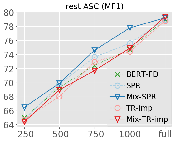
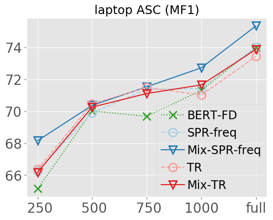
Figure 7. Two representative DA operators and their MixDA versions.

5.4. Ablation analysis with MixMatch${}^{\text{NL}}$

We analyze the effect of each component of $\mathsf{MixMatch^{NL}}$ by ablation. The results are shown in Table 7. We consider a few variants. First, we replace the $\mathsf{MixDA}$ component with regular $\mathsf{DA}$’s (the “w/o. $\mathsf{MixDA}$” row). Second, we disable the use of unlabeled data. The resulting method is equivalent to the $\mathsf{BERT\text{-}FD}$ baseline but with $\mathsf{MixUp^{NL}}$ as regularization (the 3rd row). Third, to investigate if the guessed labels by pre-mature models harm the performance, we disable label guessing for the first 3 epochs (the 4th row).

Hyper-parameters. We tune the the hyper-parameters of $\mathsf{MixMatch^{NL}}$ based on our findings with $\mathsf{MixDA}$. We choose DEL-IMP and SPR-FREQ as the $\mathsf{DA}$ operators for AE and ASC respectively. We set $(\alpha_{\text{mix}},\alpha_{\text{aug}},\lambda_{U})$ to be $(.2,.2,.1)$ for Restaurant AE, $(.2,.5,.1)$ for Laptop AE, and $(.8,.8,.25)$ for the two ASC datasets. Note that training $\mathsf{MixMatch^{NL}}$ generally takes longer time than simple fine-tuning thus we were not able to try all combinations exhaustively. For $\mathsf{MixUp^{NL}}$, we pick the best result with $\alpha$ chosen from $\{0.2,0.5,0.8\}$.

Table 7. Ablation analysis of $\mathsf{MixMatch^{NL}}$. We evaluate performance with F1 score for AE and MF1 for ASC.

Methods	AE@1000		ASC@1000		AE@full		ASC@full
	rest	laptop	rest	laptop	rest	laptop	rest	laptop
$\mathsf{MixMatch^{NL}}$	77.18	81.48	77.40	73.68	79.65	85.26	80.45	75.16
w/o. $\mathsf{MixDA}$	76.76	81.15	75.60	73.13	79.29	85.26	80.29	75.36
$\mathsf{MixUp^{NL}}$	76.15	80.69	74.78	71.46	78.07	84.70	78.32	73.00
w/o. pre-mature	76.90	81.18	77.88	74.00	79.27	85.73	80.47	75.01

Results. Table 7 shows that both $\mathsf{MixDA}$ and unlabeled data are important to $\mathsf{MixMatch^{NL}}$’s performance. The performance generally degrades as $\mathsf{MixDA}$ is removed (by up to 1.8% in Restaurant ASC@1000) and unlabeled data are removed (by up to 2.6%). The effectiveness of the two optimizations is similar among both AE and ASC tasks. As expected, both optimizations are more effective in the settings with less data (a total of 9.76% absolute improvement at size 1000 vs. 6.75% at full size). Finally, it is unclear whether discarding guessed labels from pre-mature models helps improve the performance (with only $\sim$1% difference overall).

6. Snippext in Practice

Next, we demonstrate $\mathsf{Snippext}$’s performance in practice on a real-world hotel review corpus. This hotel review corpus consists of 842,260 reviews of 494 San Francisco hotels and is collected by an online review aggregation company whom we collaborate with.

We apply $\mathsf{Snippext}$ to extract opinions/customer experiences from the hotel review corpus. We obtain labeled training datasets from (Li et al., 2019) for tagging, pairing, and attribute classificationto train $\mathsf{Snippext}$’s models for the hotel domain. In addition to their datasets, we labeled 1,500 more training examples and added 50,000 unlabeled sentences for semi-supervised learning. Since the aspect sentiment data are not publicly available for the hotel corpus, we use the restaurant ASC dataset described in Section 5. A summary of the data configurations is shown in Table 8.

We train each model as follows. All 4 models use the base BERT model fine-tuned on hotel reviews. Both the tagging and pairing models are trained using $\mathsf{MixMatch^{NL}}$ with the TR-IMP $\mathsf{DA}$ operator and $(\alpha_{\text{mix}},\alpha_{\text{aug}},\lambda_{U})=(0.2,0.8,0.5)$. For the attribute model, we use the baseline’s fine-tuning method instead of $\mathsf{MixMatch^{NL}}$ since the task is simple and there is adequate training data available. The sentiment model is trained with the best configuration described in the last section.

For each model, we repeat the training process 5 times and select the best performing model in the test set for deployment. Table 8 summarizes each model’s performance on various metrics. $\mathsf{Snippext}$’s models consistently outperform models obtained with the baseline method in (Li et al., 2019) (i.e., fine-tuned vanilla BERT) significantly. The performance improvement ranges from 1.5% (tagging F1) to 3.8% (pairing accuracy) in absolute values.

Table 8. Models for Hotel Extractions.

Tasks	Train / Test / Raw	Metrics	$\mathsf{Snippext}$	Baseline
Tagging	2,452 / 200 / 50,000	P / R / F1	71.1 / 81.0 75.7	68.9 / 80.5 74.2
Pairing	4,180 / 561 / 75,699	Acc. / F1	84.7 / 78.3	80.9 / 74.5
Attribute	4,000 / 1,000 / -	Acc. / MF1	88.0 / 86.9	86.2 / 83.3
Sentiment	3,452 / 1,120 / 35,554	Acc. / MF1	87.1 / 80.7	-

With these 4 models deployed, $\mathsf{Snippext}$ can extract 3.49M aspect-opinion tuples from the review corpus, compared to only 3.16M tuples extracted by the baseline pipeline. To better understand the coverage difference, we look into the aspect-opinion pairs extracted only by $\mathsf{Snippext}$ but not by the baseline pipeline. We list the most frequent ones in Table 9. Observe that $\mathsf{Snippext}$ extracts more fine-grained opinions. For example, “hidden, fees” appears 198 times in $\mathsf{Snippext}$’s extractions, out of 707 “fees” related extractions. In contrast, there are only 124 “fees” related extractions with the baseline method and the most frequent ones are “too many, fees”, which is less informative than “hidden fees” (and “hidden fees” are not extracted by the baseline method). As another example, there are only 95 baseline extractions about the price (i.e., contains “$” and a number) of an aspect. In comparison, $\mathsf{Snippext}$ extracts 21,738 (228$\times$ more) tuples about the price of an aspect (e.g., “$50, parking”).

Such finer-grained opinions are useful information for various applications such as opinion summarization and question answering. For example, if a user asks “Is this hotel in a good or bad location?”, then a hotel QA system can provide the general answer “Good location” and additionally, also provide finer-grained information to explain the answer (e.g., “5 min away from Fisherman’s Wharf”).

Table 9. Most frequent new opinion tuples discovered by $\mathsf{Snippext}$.

Tuples	Count	Tuples	Count
definitely recommend, hotel	1411	own, bathroom	211
going on, construction	635	only, valet parking	208
some, noise	532	many good, restaurants	199
close to, all	449	went off, fire alarm	198
great little, hotel	383	hidden, fees	198
some, street noise	349	many great, restaurants	197
only, coffee	311	excellent location, hotel	185
very happy with, hotel	286	very much enjoyed, stay	184
$ 50, parking	268	drunk, people	179
just off, union square	268	few, amenities	171
noisy at, night	266	loved, staying	165
enjoy, city	245	quiet at, night	163
hidden, review	227	some, construction	161
definitely recommend, place	217	some, homeless people	151
too much trouble, nothing	212	truly enjoyed, stay	145

7. Related Work

Structured information, such as aspects, opinions, and sentiments, which are extracted from reviews are used to support a variety of real-world applications (Archak et al., 2007; Kim et al., 2011; Marrese-Taylor et al., 2014; Li et al., 2019; Evensen et al., 2019). Mining such information is challenging and there has been extensive research on these topics (Kim et al., 2011; Liu, 2012), from document-level sentiment classification (Zhang et al., 2015; Maas et al., 2011) to the more informative Aspect-Based Sentiment Analysis (ABSA) (Pontiki et al., 2014, 2015) or Targeted ABSA (Saeidi et al., 2016). Many techniques have been proposed for review mining, from lexicon-based and rule-based approaches (Hu and Liu, 2004; Ku et al., 2006; Poria et al., 2014) to supervised learning-based approaches (Kim et al., 2011). Traditionally, supervised learning-based approaches (Jakob and Gurevych, 2010; Zhang and Liu, 2011; Mitchell et al., 2013) mainly rely on Conditional Random Fields (CRF) and require heavy feature engineering. More recently, deep learning models (Tang et al., 2015; Poria et al., 2016; Wang et al., 2017; Xu et al., 2018) and word embedding techniques have also been shown to be very effective in ABSA tasks even with little or no feature engineering. Furthermore, the performance of deep learning approaches (Xu et al., 2019; Sun et al., 2019a) can be further boosted by pre-trained language models, such as BERT (Devlin et al., 2018) and XLNet (Yang et al., 2019).

$\mathsf{Snippext}$ also leverages deep learning and pre-trained LMs to perform the review-mining-related tasks and focuses on the problem of reducing the amount of training data required. One of its strategies is to augment the available training data through data augmentation. The most popular $\mathsf{DA}$ operator in NLP is by replacing words with other words selected by random sampling (Wei and Zou, 2019), synonym dictionary (Zhang et al., 2015), semantic similarity (Wang and Yang, 2015), contextual information (Kobayashi, 2018), and frequency (Fadaee et al., 2017; Xie et al., 2019). Other operators, such as random insert/delete/swap words (Wei and Zou, 2019) and back translation (Yu et al., 2018), are also proved to be effective in text classification tasks. As naively applying these operators may produce significant distortion to the labeled data, $\mathsf{Snippext}$ proposes a set of $\mathsf{DA}$ operators suitable for opinion mining and only “partially” augments the data through $\mathsf{MixDA}$.

A common strategy in Semi-Supervised Learning (SSL) is
Expectation-Maximization (EM) (Nigam et al., 2000), which uses both labeled and unlabeled data to estimate parameters in a generative classifier, such as naive Bayes. Other strategies include self-training (Rosenberg et al., 2005; Wang et al., 2008; Sajjadi et al., 2016), which first learns an initial model from the labeled data then uses unlabeled data to further teach and learn from itself, and multi-view training (Blum and Mitchell, 1998; Zhou and Li, 2005; Xu et al., 2013; Clark et al., 2018), which extends self-training to multiple classifiers that teach and learn from each other while learning from different slices of the unlabeled data. MixMatch (Berthelot et al., 2019b, a; Song et al., 2019) is a recently proposed SSL paradigm that extends previous self-training methods by interpolating labeled and unlabeled data. MixMatch outperformed previous SSL algorithms and achieved promising results in multiple image classification tasks with only few hundreds of labels. $\mathsf{Snippext}$ uses $\mathsf{MixMatch^{NL}}$, an adaptation of MixMatch to the text setting. $\mathsf{MixMatch^{NL}}$ demonstrated SOTA results in many cases and this opens up new opportunities for leveraging the abundance of unlabeled reviews that are available on the Web. In addition to pre-training word embeddings or LMs, the unlabeled reviews can also benefit fine-tuning of LMs in obtaining more robust and generalized models (Carmon et al., 2019; Miyato et al., 2017; Hendrycks et al., 2019).

8. Conclusion

We proposed $\mathsf{Snippext}$, a semi-supervised opinion mining system that extracts aspects, opinions, and sentiments from text. Driven by the novel data augmentation technique $\mathsf{MixDA}$ and semi-supervised learning algorithm $\mathsf{MixMatch^{NL}}$, $\mathsf{Snippext}$ achieves SOTA results in multiple opinion mining tasks with only half the amount of training data used by SOTA techniques. $\mathsf{Snippext}$ is already making practical impacts on our ongoing collaboration with a hotel review aggregation platform and a job-seeking company. In the future, we will explore optimization opportunities such as multitask learning and active learning to further reduce the labeled data requirements in $\mathsf{Snippext}$.

References

- (1)
- Archak et al. (2007) Nikolay Archak, Anindya Ghose, and Panagiotis G Ipeirotis. 2007. Show me the money!: deriving the pricing power of product features by mining consumer reviews. In Proceedings of the 13th ACM SIGKDD international conference on Knowledge discovery and data mining. ACM, 56–65.
- Beltagy et al. (2019) Iz Beltagy, Arman Cohan, and Kyle Lo. 2019. Scibert: Pretrained contextualized embeddings for scientific text. arXiv preprint arXiv:1903.10676 (2019).
- Berthelot et al. (2019a) David Berthelot, Nicholas Carlini, Ekin D Cubuk, Alex Kurakin, Kihyuk Sohn, Han Zhang, and Colin Raffel. 2019a. ReMixMatch: Semi-Supervised Learning with Distribution Alignment and Augmentation Anchoring. arXiv preprint arXiv:1911.09785 (2019).
- Berthelot et al. (2019b) David Berthelot, Nicholas Carlini, Ian Goodfellow, Nicolas Papernot, Avital Oliver, and Colin Raffel. 2019b. Mixmatch: A holistic approach to semi-supervised learning. arXiv preprint arXiv:1905.02249 (2019).
- Blum and Mitchell (1998) Avrim Blum and Tom Mitchell. 1998. Combining labeled and unlabeled data with co-training. In Proceedings of the eleventh annual conference on Computational learning theory. Citeseer, 92–100.
- Carmon et al. (2019) Yair Carmon, Aditi Raghunathan, Ludwig Schmidt, John C. Duchi, and Percy Liang. 2019. Unlabeled Data Improves Adversarial Robustness. In Advances in Neural Information Processing Systems (NeurIPS) 2019. 11190–11201.
- Clark et al. (2018) Kevin Clark, Minh-Thang Luong, Christopher D Manning, and Quoc V Le. 2018. Semi-supervised sequence modeling with cross-view training. arXiv preprint arXiv:1809.08370 (2018).
- Cubuk et al. (2018) Ekin D Cubuk, Barret Zoph, Dandelion Mane, Vijay Vasudevan, and Quoc V Le. 2018. Autoaugment: Learning augmentation policies from data. arXiv preprint arXiv:1805.09501 (2018).
- Devlin et al. (2018) Jacob Devlin, Ming-Wei Chang, Kenton Lee, and Kristina Toutanova. 2018. Bert: Pre-training of deep bidirectional transformers for language understanding. arXiv preprint arXiv:1810.04805 (2018).
- Evensen et al. (2019) Sara Evensen, Aaron Feng, Alon Halevy, Jinfeng Li, Vivian Li, Yuliang Li, Huining Liu, George Mihaila, John Morales, Natalie Nuno, et al. 2019. Voyageur: An Experiential Travel Search Engine. In The World Wide Web Conference. ACM, 3511–5.
- Fadaee et al. (2017) Marzieh Fadaee, Arianna Bisazza, and Christof Monz. 2017. Data augmentation for low-resource neural machine translation. arXiv preprint arXiv:1705.00440 (2017).
- Guo et al. (2019) Hongyu Guo, Yongyi Mao, and Richong Zhang. 2019. Augmenting Data with Mixup for Sentence Classification: An Empirical Study. arXiv preprint arXiv:1905.08941 (2019).
- He and McAuley (2016) Ruining He and Julian McAuley. 2016. Ups and downs: Modeling the visual evolution of fashion trends with one-class collaborative filtering. In WWW. 507–517.
- Hendrycks et al. (2019) Dan Hendrycks, Norman Mu, Ekin D Cubuk, Barret Zoph, Justin Gilmer, and Balaji Lakshminarayanan. 2019. AugMix: A Simple Data Processing Method to Improve Robustness and Uncertainty. arXiv preprint arXiv:1912.02781 (2019).
- Hu and Liu (2004) Minqing Hu and Bing Liu. 2004. Mining and summarizing customer reviews. In Proceedings of the tenth ACM SIGKDD international conference on Knowledge discovery and data mining. ACM, 168–177.
- Jakob and Gurevych (2010) Niklas Jakob and Iryna Gurevych. 2010. Extracting opinion targets in a single-and cross-domain setting with conditional random fields. In Proceedings of the 2010 conference on empirical methods in natural language processing. Association for Computational Linguistics, 1035–1045.
- Kim et al. (2011) Hyun Duk Kim, Kavita Ganesan, Parikshit Sondhi, and ChengXiang Zhai. 2011. Comprehensive review of opinion summarization. Technical Report.
- Kobayashi (2018) Sosuke Kobayashi. 2018. Contextual augmentation: Data augmentation by words with paradigmatic relations. arXiv preprint arXiv:1805.06201 (2018).
- Ku et al. (2006) Lun-Wei Ku, Yu-Ting Liang, and Hsin-Hsi Chen. 2006. Opinion extraction, summarization and tracking in news and blog corpora. In Proceedings of AAAI. 100–107.
- Lee et al. (2019) Jinhyuk Lee, Wonjin Yoon, Sungdong Kim, Donghyeon Kim, Sunkyu Kim, Chan Ho So, and Jaewoo Kang. 2019. Biobert: pre-trained biomedical language representation model for biomedical text mining. arXiv preprint arXiv:1901.08746 (2019).
- Li et al. (2016) Guoliang Li, Jiannan Wang, Yudian Zheng, and Michael J Franklin. 2016. Crowdsourced data management: A survey. IEEE Transactions on Knowledge and Data Engineering 28, 9 (2016), 2296–2319.
- Li et al. (2019) Yuliang Li, Aaron Xixuan Feng, Jinfeng Li, Saran Mumick, Alon Halevy, Vivian Li, and Wang-Chiew Tan. 2019. Subjective Databases. PVLDB 12, 11 (2019), 1330–1343.
- Liu (2012) Bing Liu. 2012. Sentiment Analysis and Opinion Mining. Morgan & Claypool.
- Maas et al. (2011) Andrew L Maas, Raymond E Daly, Peter T Pham, Dan Huang, Andrew Y Ng, and Christopher Potts. 2011. Learning word vectors for sentiment analysis. In Proceedings of the 49th annual meeting of the association for computational linguistics: Human language technologies-volume 1. Association for Computational Linguistics, 142–150.
- Marrese-Taylor et al. (2014) Edison Marrese-Taylor, Juan D Velásquez, and Felipe Bravo-Marquez. 2014. A novel deterministic approach for aspect-based opinion mining in tourism products reviews. Expert Systems with Applications 41, 17 (2014), 7764–7775.
- Mikolov et al. (2013) Tomas Mikolov, Kai Chen, Greg Corrado, and Jeffrey Dean. 2013. Efficient estimation of word representations in vector space. arXiv preprint arXiv:1301.3781 (2013).
- Mitchell et al. (2013) Margaret Mitchell, Jacqui Aguilar, Theresa Wilson, and Benjamin Van Durme. 2013. Open domain targeted sentiment. In Proceedings of the 2013 Conference on Empirical Methods in Natural Language Processing. 1643–1654.
- Miyato et al. (2017) Takeru Miyato, Andrew M. Dai, and Ian J. Goodfellow. 2017. Adversarial Training Methods for Semi-Supervised Text Classification. In 5th International Conference on Learning Representations, ICLR 2017.
- Nigam et al. (2000) Kamal Nigam, Andrew Kachites McCallum, Sebastian Thrun, and Tom Mitchell. 2000. Text classification from labeled and unlabeled documents using EM. Machine learning 39, 2-3 (2000), 103–134.
- Perez and Wang (2017) Luis Perez and Jason Wang. 2017. The effectiveness of data augmentation in image classification using deep learning. arXiv preprint arXiv:1712.04621 (2017).
- Pontiki et al. (2016) Maria Pontiki, Dimitris Galanis, Haris Papageorgiou, Ion Androutsopoulos, Suresh Manandhar, AL-Smadi Mohammad, Mahmoud Al-Ayyoub, Yanyan Zhao, Bing Qin, Orphée De Clercq, et al. 2016. SemEval-2016 task 5: Aspect based sentiment analysis. In SemEval-2016. 19–30.
- Pontiki et al. (2015) Maria Pontiki, Dimitris Galanis, Haris Papageorgiou, Suresh Manandhar, and Ion Androutsopoulos. 2015. Semeval-2015 task 12: Aspect based sentiment analysis. In Proceedings of the 9th International Workshop on Semantic Evaluation (SemEval 2015). 486–495.
- Pontiki et al. (2014) Maria Pontiki, Dimitris Galanis, John Pavlopoulos, Harris Papageorgiou, Ion Androutsopoulos, and Suresh Manandhar. 2014. SemEval-2014 Task 4: Aspect Based Sentiment Analysis. In Proceedings of the 8th International Workshop on Semantic Evaluation (SemEval 2014). 27–35.
- Poria et al. (2016) Soujanya Poria, Erik Cambria, and Alexander Gelbukh. 2016. Aspect extraction for opinion mining with a deep convolutional neural network. Knowledge-Based Systems 108 (2016), 42–49.
- Poria et al. (2014) Soujanya Poria, Erik Cambria, Lun-Wei Ku, Chen Gui, and Alexander Gelbukh. 2014. A rule-based approach to aspect extraction from product reviews. In Proceedings of the second workshop on natural language processing for social media (SocialNLP). 28–37.
- Radford et al. (2018) Alec Radford, Karthik Narasimhan, Tim Salimans, and Ilya Sutskever. 2018. Improving language understanding by generative pre-training. URL https://s3-us-west-2. amazonaws. com/openai-assets/researchcovers/languageunsupervised/language understanding paper. pdf (2018).
- Rosenberg et al. (2005) Chuck Rosenberg, Martial Hebert, and Henry Schneiderman. 2005. Semi-Supervised Self-Training of Object Detection Models. WACV/MOTION 2 (2005).
- Saeidi et al. (2016) Marzieh Saeidi, Guillaume Bouchard, Maria Liakata, and Sebastian Riedel. 2016. Sentihood: Targeted aspect based sentiment analysis dataset for urban neighbourhoods. arXiv preprint arXiv:1610.03771 (2016).
- Sajjadi et al. (2016) Mehdi Sajjadi, Mehran Javanmardi, and Tolga Tasdizen. 2016. Regularization with stochastic transformations and perturbations for deep semi-supervised learning. In Advances in Neural Information Processing Systems. 1163–1171.
- Settles (2009) Burr Settles. 2009. Active learning literature survey. Technical Report. University of Wisconsin-Madison Department of Computer Sciences.
- Settles et al. (2008) Burr Settles, Mark Craven, and Lewis Friedland. 2008. Active learning with real annotation costs. In Proceedings of the NIPS workshop on cost-sensitive learning. Vancouver, CA, 1–10.
- Song et al. (2019) Shuang Song, David Berthelot, and Afshin Rostamizadeh. 2019. Combining MixMatch and Active Learning for Better Accuracy with Fewer Labels. arXiv preprint arXiv:1912.00594 (2019).
- Sun et al. (2019a) Chi Sun, Luyao Huang, and Xipeng Qiu. 2019a. Utilizing BERT for Aspect-Based Sentiment Analysis via Constructing Auxiliary Sentence. arXiv preprint arXiv:1903.09588 (2019).
- Sun et al. (2019b) Chi Sun, Luyao Huang, and Xipeng Qiu. 2019b. Utilizing BERT for Aspect-Based Sentiment Analysis via Constructing Auxiliary Sentence. arXiv preprint arXiv:1903.09588 (2019).
- Tang et al. (2015) Duyu Tang, Bing Qin, and Ting Liu. 2015. Document modeling with gated recurrent neural network for sentiment classification. In Proceedings of the 2015 conference on empirical methods in natural language processing. 1422–1432.
- Verma et al. (2018) Vikas Verma, Alex Lamb, Christopher Beckham, Aaron Courville, Ioannis Mitliagkis, and Yoshua Bengio. 2018. Manifold mixup: Encouraging meaningful on-manifold interpolation as a regularizer. stat 1050 (2018), 13.
- Wang et al. (2008) Bin Wang, Bruce Spencer, Charles X Ling, and Harry Zhang. 2008. Semi-supervised self-training for sentence subjectivity classification. In Conference of the Canadian Society for Computational Studies of Intelligence. Springer, 344–355.
- Wang et al. (2016) Wenya Wang, Sinno Jialin Pan, Daniel Dahlmeier, and Xiaokui Xiao. 2016. Recursive Neural Conditional Random Fields for Aspect-based Sentiment Analysis. In EMNLP. 616–626.
- Wang et al. (2017) Wenya Wang, Sinno Jialin Pan, Daniel Dahlmeier, and Xiaokui Xiao. 2017. Coupled Multi-Layer Attentions for Co-Extraction of Aspect and Opinion Terms.. In AAAI. 3316–3322.
- Wang and Yang (2015) William Yang Wang and Diyi Yang. 2015. That’s so annoying!!!: A lexical and frame-semantic embedding based data augmentation approach to automatic categorization of annoying behaviors using# petpeeve tweets. In Proceedings of the 2015 Conference on Empirical Methods in Natural Language Processing. 2557–2563.
- Wei and Zou (2019) Jason W Wei and Kai Zou. 2019. Eda: Easy data augmentation techniques for boosting performance on text classification tasks. arXiv preprint arXiv:1901.11196 (2019).
- Xie et al. (2019) Qizhe Xie, Zihang Dai, Eduard Hovy, Minh-Thang Luong, and Quoc V Le. 2019. Unsupervised data augmentation. arXiv preprint arXiv:1904.12848 (2019).
- Xu et al. (2013) Chang Xu, Dacheng Tao, and Chao Xu. 2013. A survey on multi-view learning. arXiv preprint arXiv:1304.5634 (2013).
- Xu et al. (2018) Hu Xu, Bing Liu, Lei Shu, and Philip S Yu. 2018. Double embeddings and cnn-based sequence labeling for aspect extraction. arXiv preprint arXiv:1805.04601 (2018).
- Xu et al. (2019) Hu Xu, Bing Liu, Lei Shu, and Philip S Yu. 2019. Bert post-training for review reading comprehension and aspect-based sentiment analysis. arXiv preprint arXiv:1904.02232 (2019).
- Yang et al. (2019) Zhilin Yang, Zihang Dai, Yiming Yang, Jaime Carbonell, Ruslan Salakhutdinov, and Quoc V Le. 2019. XLNet: Generalized Autoregressive Pretraining for Language Understanding. arXiv preprint arXiv:1906.08237 (2019).
- Yelp_Dataset ([n.d.]) Yelp_Dataset. [n.d.]. https://www.yelp.com/dataset.
- Yu et al. (2018) Adams Wei Yu, David Dohan, Minh-Thang Luong, Rui Zhao, Kai Chen, Mohammad Norouzi, and Quoc V Le. 2018. Qanet: Combining local convolution with global self-attention for reading comprehension. arXiv preprint arXiv:1804.09541 (2018).
- Zhang et al. (2017) Hongyi Zhang, Moustapha Cisse, Yann N Dauphin, and David Lopez-Paz. 2017. mixup: Beyond empirical risk minimization. arXiv preprint arXiv:1710.09412 (2017).
- Zhang and Liu (2011) Lei Zhang and Bing Liu. 2011. Extracting resource terms for sentiment analysis. In Proceedings of 5th International Joint Conference on Natural Language Processing. 1171–1179.
- Zhang et al. (2015) Xiang Zhang, Junbo Zhao, and Yann LeCun. 2015. Character-level convolutional networks for text classification. In NeurIPS. 649–657.
- Zhou and Li (2005) Zhi-Hua Zhou and Ming Li. 2005. Tri-training: Exploiting unlabeled data using three classifiers. IEEE Transactions on Knowledge & Data Engineering 11 (2005), 1529–1541.
- Zhu (2005) Xiaojin Jerry Zhu. 2005. Semi-supervised learning literature survey. Technical Report. University of Wisconsin-Madison Department of Computer Sciences.