Parallel PERM

Abstract

We develop and implement a parallel flatPERM algorithm [8, 12] with mutually interacting parallel flatPERM sequences and use it to sample self-avoiding walks in 2 and 3 dimensions. Our data show that the parallel implementation accelerates the convergence of the flatPERM algorithm. Moreover, increasing the number of interacting flatPERM sequences (rather than running longer simulations) improves the rate of convergence. This suggests that a more efficient implementation of flatPERM will be a massively parallel implementation, rather than long simulations of one, or a few parallel sequences. We also use the algorithm to estimate the growth constant of the self-avoiding walk in two and in three dimensions using simulations over 12 parallel sequences. Our best results are

$$\mu_{d}=\cases{2.6381585(1),&\hbox{if $d=2$};\cr 4.684039(1),&\hbox{if $d=3$}.}$$

Keywords: PERM, flatPERM, Parallel Computing, Rosenbluth Method, Self-avoiding Walk

1 Introduction

The Rosenbluth algorithm [9, 14] samples self-avoiding walks by recursively appending steps at the end of the walk. Since the sampling is not uniform, the algorithm continuously updates a weight function which is used for determining averages of observables with respect to the uniform distribution over walks of length $n$ from the origin.

More precisely, let ${\mathbb{S}}$ be the state space of self-avoiding walks from the origin $\vec{0}$ in the $d$-dimensional hypercubic lattice ${\mathbb{Z}}^{d}$, and denote the walk composed of the single vertex $\vec{0}$ and of length $0$ by $\emptyset$. Suppose a walk $\omega_{n}$ of length $n$ steps have been grown recursively, then append the next step as follows: Let $a_{+}(\omega_{n})$ be the number of possible (steps) edges incident with the end-point of the $\omega_{n}$ which may be appended to $\omega_{n}$ to get a walk $\omega_{n+1}$ of length $n+1$. Choose one of these edges uniformly, and append it to $\omega_{n}$ to obtain $\omega_{n+1}$. Recursive implementation of this generates a sequence (or chain) of walks $\left\langle\emptyset,\omega_{1},\omega_{2},\ldots,\omega_{n},\ldots\right\rangle$, which we shall also call a chain (realised by the algorithm), and where $\omega_{n}$ is a prefix of $\omega_{n+1}$.

Since $a_{+}(\emptyset)=2d$, the probability of adding one step to grow the walk $\omega_{1}$ of length one from $\emptyset$ is ${\hbox{P}_{\hskip-2.84526ptr}}(\emptyset\to\omega_{1})=\hbox{\large$\frac{1}{2d}$}$. More generally, the probability of obtaining a walk $\omega_{n+1}$ of length $n+1$ from a walk $\omega_{n}$ of length $n$ is ${\hbox{P}_{\hskip-2.84526ptr}}(\omega\to\omega_{n+1})=\hbox{\large$\frac{1}{a_{+}(\omega_{n})}$}\,{\hbox{P}_{\hskip-2.84526ptr}}(\omega_{n})$.

The probability of a particular sequence of walks $S_{n}=\left\langle\emptyset,\omega_{1},\omega_{2},\ldots,\omega_{n}\right\rangle$ being realised by the algorithm is

$${\hbox{P}_{\hskip-2.84526ptr}}(S_{n})=\prod_{j=1}^{n}{\hbox{P}_{\hskip-2.84526ptr}}(\omega_{j-1}\to\omega_{j})=\prod_{k=0}^{n-1}\hbox{\large$\frac{1}{a_{+}(\omega_{k})}$}$$ (1)

where $\omega_{0}=\emptyset$.

The weight of the sequence $S_{n}$ is defined by

$$W(S_{n})=\hbox{\large$\frac{1}{\footnotesize{{\hbox{P}_{\hskip-2.84526ptr}}(S_{n})}}$}=\prod_{k=0}^{n-1}a_{+}(\omega_{k}).$$ (2)

The function $W(S_{n})$ is an observable, and its exact value for walks of length $n$, computed over all sequences of walks $S$ of length $|S|=n$ is

$$W_{n}=\sum_{S:|S|=n}{\hbox{P}_{\hskip-2.84526ptr}}(S)\,W(S)=\sum_{S:|S|=n}\left({\hbox{P}_{\hskip-2.84526ptr}}(S)\times\hbox{\large$\frac{1}{\footnotesize{{\hbox{P}_{\hskip-2.84526ptr}}(S)}}$}\right)=\sum_{S:|S|=n}{\LARGE 1}=c_{n},$$ (3)

where $c_{n}$ is the number of walks of length $n$ from the origin and since each sequence $S$ of length $n$ ends in exactly one unique walk. Equation (3) is the Rosenbluth counting theorem. Estimating $W_{n}$ using the algorithm gives approximations of $c_{n}$, so that the Rosenbluth algorithm is an approximate enumeration algorithm. Since the algorithm grows walks recursively, there is a non-zero probability that a growing walk $\omega_{n}$ can be trapped (this occurs when $a_{+}(\omega_{n})=0$) in which case ${\hbox{P}_{\hskip-2.84526ptr}}(\omega_{n}\to\omega^{\prime})=0$. Any realised sequence or a chain which grow to include the trapped state $\omega_{n}$ is terminated, and the (hypothetical) subsequent states following $\omega_{n}$ are assigned the default weight zero. Since any self-avoiding walk of length $n$ can be grown by the algorithm, this algorithm is irreducible.

Implementation of the algorithm to grow walks of length $n$ gives a set of independently grown walks of length $n$ denoted by $\{\sigma_{1},\sigma_{2},\ldots,\sigma_{M}\}$ with weights $W_{n}(\sigma_{j})$. Since there are trapped states, for some $\sigma_{k}$ it may be the case that $W_{n}(\sigma_{k})=0$. The sample average of $W_{n}(\sigma)$ is

$$\left[W_{n}\right]_{M}^{sample}=\hbox{\normalsize$\frac{1}{M}$}\sum_{i=1}^{M}W_{n}({\sigma_{i}})=\hbox{\large$\frac{\sum_{i=1}^{M}W_{n}({\sigma_{i}})}{\sum_{i=1}^{M}W_{0}({\sigma_{i}})}$},$$ (4)

since $W_{0}({\sigma_{i}})=1$ and where $M$ is the number of sequences started by the algorithm (or more accurately, the number of times the sequence passes through the empty walk and restarts the sampling of a new walk), and $W_{n}({\sigma_{i}})$ is the weight of the state ${\sigma_{i}}$. By the strong law of large numbers one expects that $\left[W_{n}\right]_{M}^{sample}$ converges to $W_{n}=c_{n}$ as $M\to\infty$ (see equation (3)).

The estimator $\left[{\mathcal{O}}\right]_{M}^{est}$ over a set of $M$ walks realised by the algorithm for the (canonical) average of an observable ${\mathcal{O}}(\omega)$ over the uniform distribution of self-avoiding walks of length $n$ can computed using a ratio estimator:

$$\left[{\mathcal{O}}\right]_{M}^{est}=\frac{\sum_{i=1}^{M}W_{i}({\sigma_{i}}){\hskip 0.75pt}{\mathcal{O}}({\sigma_{i}})}{\sum_{i=1}^{M}W_{i}({\sigma_{i}})}=\frac{\left[W{\mathcal{O}}\right]_{M}^{sample}}{\left[W\right]_{M}^{sample}}.$$ (5)

As $M\to\infty$, then $\left[{\mathcal{O}}\right]_{M}^{est}\to\left\langle{\mathcal{O}}\right\rangle$.

In this paper the feasibility of a parallel implementation of algorithms based on Rosenbluth sampling (namely the PERM and flatPERM algorithms) is considered. The increasing parallel architecture of modern computers suggests that future improvements in performance will be obtained by implementing parallel versions of these algorithms, and such implementations may also bring improvements in convergence in the same way that gains were made by the introduction of multiple chains in parallel in Metropolis Monte Carlo methods [16]. In the next section we briefly review PERM and flatPERM, and in section 3 we explain a parallel implementation of these algorithms. This implementation is simple, and proceeds by seeding multiple PERM sequences in parallel (one per thread or CPU) and then collecting and sharing data between all the sequences as they evolve in real time.

We test the parallel implementation and its performance in a variety of ways in section 3, including estimating $c_{10,000}$ (the number of self-avoiding walks of length $10,000$), a total absolute error for simulations of walks up to length $10,\!000$, and estimating the least squares error and growth constant $\mu_{d}$ and entropic exponent $\gamma$ for self-avoiding walks. In section 4 we conclude the paper with a few final observations.

2 PERM and flatPERM

The Rosenbluth algorithm samples walks of moderate lengths (say up to length $100$) very efficiently, but the attrition of walks due to trapped conformations in low dimensions, and the increasing dispersion of weights over a wide range of orders of magnitude as walks grow in length, quickly degrade estimators as $n$ increases (see equation (5)). As a result, alterations to the algorithm to compensate for the dispersion of weights, and attrition of walks, have been introduced. These are variance reduction methods and they have greatly improved the performance of the Rosenbluth algorithm.

The first variance reduction method is due to Meirovitch [11], and is called the scanning method. Its implementation is not difficult, and it greatly improves the efficiency of Rosenbluth sampling by both dealing with the dispersion of weights and with attrition of walks due to trapped conformations. The second variance reduction method is due to Grassberger [8] (PERM), and a variant of this due to Prellberg and Krawczyk [12] (flatPERM) samples asymptotically over flat histograms over state space (flatPERM is also an example of rare event sampling).

The PERM and flatPERM implementation of the Rosenbluth algorithm are based on ideas of pruning and enrichment of states with low and high weights respectively [17, 7]. These implementations were also generalised in the flatGARM algorithm which is a more general algorithm based on Rosenbluth style sampling [13].

Suppose that a walk of length $n$ was grown using the Rosenbluth algorithm by appending steps starting at the empty walk along a sequence $\left\langle{\omega_{0}},{\omega_{1}},\ldots,{\omega_{n}}\right\rangle$ (where ${\omega_{0}}=\emptyset$). The weight of state ${\omega_{k}}$ is denoted by $W({\omega_{k}})$ and is given by equation (2) where $S_{k}=\left\langle{\omega_{0}},{\omega_{1}},\ldots,{\omega_{k}}\right\rangle$ so that $W({\omega_{k}})\equiv W(S_{k})$.

Introduce a cut-off $T_{k}$ on $W({\omega_{k}})$ for walks of length $k$. If $W({\omega_{k}})>T_{k}$, then enrich ${\omega_{k}}$ in $S_{k}$ by adding $M$ copies of ${\omega_{k}}$ to $S_{k}$ and by reducing (dividing) $W({\omega_{k}})$ by a factor of $M$. The algorithm then continues to grow $M$ walks from ${\omega_{k}}$ independently with reduced weights, in each case continually enriching states if their weights similarly exceed the cut-off $T_{k}$. This enrichment and weight reduction of states with large weights have the effect of reducing the dispersion of weights systematically. Enriching states also does not disturb the sample average of observables.

A state ${\omega_{k}}$ with a small weight can be pruned by removing it from $S$ and assigning it zero weight. This is implemented by introducing a lower cut-off $t_{k}$ at length $k$ on $W({\omega_{k}})$. If $W({\omega_{k}})<t_{k}$, then the walk is pruned with probability $1{\hskip 0.85pt{-}\hskip 0.85pt}\hbox{\normalsize$\frac{1}{q}$}$ where $q$ is a parameter of the algorithm. If the walk is not pruned (with probability $\frac{1}{q}$), then its weight is increased by a factor of $q$. Similarly to enrichment, pruning a state with low weight does not disturb sample averages.

The dispersion of the weights $W(S_{n})$ in PERM may be further reduced by taking the cut-offs in its implementation to be equal ($t_{k}=T_{k}$) and then to continually enrichment and prune states exceeding or falling below the cut-off. This is implemented as follows: Let $[W_{k}]_{M}^{sample}$ be the running average of the weights of walks of length $k$ after $M$ sequences were realised by the algorithm. If the walk ${\omega_{k}}$ in the $M$-th sequence has PERM weight $W({\omega_{k}})$, then compute the ratio

$$r=\frac{W({\omega_{k}})}{[W_{k}]_{M}^{sample}},$$ (6)

and where the weight $W({\omega_{k}})$ is also included in the calculation of $[W_{k}]_{M}^{sample}$. The value of $[W_{k}]_{M}^{sample}$ serves as a cut-off. If $r>1$ then the weight $W({\omega_{k}})$ exceeds its expected value, and the state may be enriched, and if $r<1$ then the state has lower than expected weight, and may be pruned.

If $r\geq 1$ then the state could be enriched. Compute probability $p={\left\lceil r\right\rceil}{\hskip 0.85pt{-}\hskip 0.85pt}r$ and put $c=\!\left\lfloor r\right\rfloor\!$ with probability $p$ and with default $c=\left\lceil r\right\rceil$. Place $c$ copies of ${\omega_{k}}$ in the sequence, each with reduced weight $\hbox{\normalsize$\frac{1}{c}$}W({\omega_{k}})$. Continue to grow the sequence from each of these states independently, and at each iteration, determine $r$ as above.

If $r<1$ then $W({\omega_{k}})$ is smaller than expected. Prune it with probability $1-r$. If it is not pruned, then increase $W({\omega_{k}})$ by multiplying it with $\frac{1}{r}$.

In flatPERM simulations the running average $[W_{k}]_{M}^{sample}$ of weights is initially poor but improves quickly, and the sampling stabilizes to flat histogram sampling. There are very low attrition of sequences, and the variance reduction in flatPERM gives a quickly convergent algorithm sampling over weights in a narrow range.

................................................................................................................................................................................................................................................................................................................................................................................................................................................................................................................................................................................................................................................................................................................................................................................................................................................................................................................................................................................................................................................................................................................................................................................................................................................................................................................$\bullet$$\bullet$$\bullet$$\bullet$$\bullet$$\bullet$............................................................................................................................................................................................................$1$$2$$3$$N$$W_{1}$$W_{2}$$W_{3}$$W_{N}$....................................................................................................................................................................................................................................................................................................................................................................................................................................................................................................................................................................................................................................................................................................................................................................................................................................................................................................$\bullet$$\bullet$$\bullet$...................................................................................................................................................................................................................................................................................................................................................123$N$ W

Figure 1: Parallel implementation of PERM. Algorithm 1: On the left $N$ independent PERM sequences sample independent walks with sample averages of weights $[W_{k}]^{sample}_{M}$ independently computed for each sequence. Enrichment and pruning of states are independently done in each sequence. Algorithm 2: On the right the $N$ sequences are interacting with each other by sharing collected weights (running averages of weights) in a single data location $W$. Enrichment and pruning of states in each sequence are done by comparing weights with the sample average of the weights computed over data collected over the $N$ sequences, including the data from partially completed sequences. In both algorithms each sequence is realised in its own CPU (or thread) in the computer and runs simultaneously with other sequences. While running averages of weights are quarantined in each realised sequence in Algorithm 1, in Algorithm 2 the weights are pooled into a shared data structure $W$ while each sequence is sampling along its own thread while accessing the pooled data to calculate enrichment and pruning parameters $p$ and $r$. The CPU times of Algorithms 1 and 2 are virtually the same for the same number of parallel sequences and iterations (or started walks).

3 Parallel PERM

Two parallel implementations of the PERM algorithm are shown in figure 1. We consider them in turn

Algorithm 1: On the left $N$ independent realisations of the algorithm (1 per CPU or per thread) are initiated. The $\ell$-th realisation calculates a sample average of weights $[W_{k}]^{sample}_{M,\ell}$ for $\ell=1,2,\ldots,N$ given by equation (4). The average over the $N$ parallel sequences is

$$[W_{k}]^{(\hbox{\scriptsize alg 1})}_{M,N}=\hbox{\large$\frac{1}{N}$}\sum_{\ell=1}^{N}[W_{k}]^{sample}_{M,\ell}$$ (7)

where $M$ is the length of each sequence, and $k$ is the length of the walk. By the strong law of large numbers, $[W_{k}]^{parallel}_{M,N}$ converges to $c_{k}$ if $M\to\infty$. The convergence is accelerated if $N$ is increased (that is, when more sequences are initiated in parallel).

Algorithm 2: An integrated parallel implementation of $N$ realised PERM sequences sharing data is shown on the right in figure 1. As opposed to the implementation on the left, this is a true parallel implementation in that the $N$ parallel sequences are not independent of each other, but communicate continuously by accessing data generated by all other sequences. These shared data are used to determine the enrichment and pruning in each of the parallel sequences, and each sequence is continuously updating the shared data as it progresses. The average weights in this case are denoted by $[W_{k}]^{(\hbox{\scriptsize alg 2})}_{M,N}$ and it is computed by using equation (4) (where $M$ is now the total number of passes of all sequence through the trivial walk of length zero).

The flatPERM algorithm was implemented using both Algorithm 1 and Algorithm 2 to sample along multiple sequences. In both implementations the algorithms were coded in $C$ with open-mp protocols [1] to access CPUs and to place one PERM sequence per thread. These algorithms were run on a desktop workstation and tested for convergence in various ways. Our results are shown below.

3.1 Estimating $c_{10,000}$

In table 1 the results for simulations with two sequences are shown. The number of started walks (iterations) is given in the top row (this is the total number of walks generated – since there are two sequences the number of walks per CPU is given by the powers of $10$ in each case). Estimates of $\log c_{10,000}$ were made by calculating the average weights of the realised sequences. In Algorithm 1 an estimate was obtained for each independent sequence, and the best estimate was calculated by taking the geometric average of the estimates from each sequence. In the case of Algorithm 2 there is only one set of data collected over all sequences, and the estimate of $\log c_{10,000}$ was obtained in this case by estimating the weight over all the pooled data. These estimates are listed in the third row of table 1.

Table 1: $\log c_{10,000}$ estimated using $2$ sequences

#Walks	$2\times 1$	$2\times 10$	$2\times 10^{2}$	$2\times 10^{3}$	$2\times 10^{4}$	$2\times 10^{5}$
Alg. 1	$9226.07$	$9601.69$	$9658.76$	$9701.30$	$9704.15$	$9704.11$
Alg. 2	$9491.40$	$9644.84$	$9702.71$	$9705.09$	$9703.88$	$9704.13$

The estimate by Algorithm 1 settles down by $2\times 10^{4}$ iterations (started walks) at a value close to $9704$. By increasing the number of iterations by a factor of $10$ each along the columns of the first row, the estimate in the second row is seen to increase as the simulation proceeds before it levels off. A similar pattern is seen for Algorithm 2 – however, it levels off close to $9704$ already by $10^{2}$ walks, and more definitely by $10^{3}$. This is a factor of $10$ faster than the convergence seen in Algorithm 1. These data and results seem to imply that Algorithm 2 gives a gain of a factor of about $10$ in convergence of the approximate estimates of $c_{10,000}$ in simulations which sample walks up to length $10^{4}$. For comparison, a very long simulation using flatPERM ($1.6\times 10^{9}$ iterations) gives the estimate

$$\log c_{10,000}=9704.14\ldots$$ (8)

in the square lattice.

Similar results are seen when more sequences are used in the simulations. In table 2 results similar to those in table 1 are shown, but now for walks sampled using $12$ sequences. These results again level off with increasing number of walks, and again a large gain is seen for Algorithm 2. By $12\times 10$ walks the estimate is within $7$ of the value in equation (8), while for Algorithm 1 it is still about $65$ below.

Table 2: $\log c_{10,000}$ estimated using $12$ sequences

#Walks	$12\times 1$	$12\times 10$	$12\times 10^{2}$	$12\times 10^{3}$	$12\times 10^{4}$	$12\times 10^{5}$
Alg. 1	$9273.79$	$9658.79$	$9692.63$	$9703.54$	$9704.38$	$9704.11$
Alg. 2	$9652.09$	$9697.79$	$9703.23$	$9704.04$	$9704.16$	$9704.18$

The results in tables 1 and 2 show that Algorithm 2 outperforms Algorithm 1 substantially in particular at the initial stage of the algorithm (after a few walks have been sampled). Convergence of Algorithm 1 appears to occur when the number of iterations (started walks) approach about $12\times 10^{4}$ while Algorithm 2 is already close to its target after $12\times 10^{2}$ iterations. This shows a substantial increase in the rate of convergence of flatPERM with the introduction of coupling between sequences as proposed in Algorithm 2. In addition, the results for Algorithm 2 in tables 1 and 2 show that increasing the number of sequences from two to twelve improves the results for lower number of walks, as expected. A similar gain is seen for Algorithm 1, but not to the same degree.

3.2 Total absolute error

We define the total absolute error per unit length of $\log c_{n}$ by

$$T_{M}=\hbox{\normalsize$\frac{1}{M}$}\sum_{n=1}^{M}\left|\log c_{n}^{best}-\log c_{n}^{est}\right|$$ (9)

where $c_{n}^{best}$ is the best estimates of $c_{n}$ and $c_{n}^{est}$ is the estimate for $c_{n}$ obtained by either algorithm 1 or algorithm 2. $M$ is the maximum length of walks sampled by the algorithms.

Good estimates for $c_{n}^{best}$ are obtained from a very long (ordinary) flatPERM simulation of $1.6\times 10^{9}$ iterations. For $c_{n}^{est}$ the average weights $[W_{k}]^{(\hbox{\scriptsize alg 1})}_{M,N}$ and $[W_{k}]^{(\hbox{\scriptsize alg 2})}_{M,N}$ are used respectively, and in each case $T_{M}$ will be an estimate of the total deviation per unit length of the estimates from the best values $\log c_{n}^{best}$. For example, determining $T_{M}$ from one sequence growing a single walk with the flatPERM algorithm gives a total absolute error per unit length of $239.33$ for walks of length up to $M=10,000$.

The results are shown in table 3 for both algorithms and for lengths of walks up to $10^{4}$. The first column gives the number of started walks per sequence for each algorithm ($S$). The columns under Algorithm 1 shows $T_{10,000}$ as measured using equation (9). For example, a simulation of Algorithm 1 using 2 sequences for $1$ started walk each gives the total absolute error $231.79$, as seen in the column $N=2$ under algorithm 1, while using two sequences in parallel in Algorithm 2 gives $113.17$, a significant reduction as seen in the column $N=2$ under Algorithm 2, especially at lower numbers of started walks.

Table 3: $T_{10,000}$

	Algorithm 1					Algorithm 2
S	$N=1$	$N=2$	$N=3$	$N=6$	$N=12$	$N=2$	$N=3$	$N=6$	$N=12$
$1$	$239.33$	$231.79$	$224.73$	$213.67$	$200.88$	$113.17$	$108.71$	$44.81$	$20.38$
$10$	$69.34$	$47.22$	$47.53$	$48.19$	$22.26$	$32.49$	$13.58$	$8.01$	$2.89$
$10^{2}$	$30.72$	$23.61$	$14.39$	$6.65$	$5.59$	$1.120$	$0.716$	$0.500$	$0.339$
$10^{3}$	$3.217$	$1.284$	$1.256$	$0.696$	$0.220$	$0.620$	$0.812$	$0.393$	$0.280$
$10^{4}$	$0.383$	$0.197$	$0.0920$	$0.271$	$0.145$	$0.190$	$0.0767$	$0.0657$	$0.0459$
$10^{5}$	$0.0446$	$0.0387$	$0.0466$	$0.0481$	$0.0310$	$0.0519$	$0.0928$	$0.0188$	$0.0144$
$10^{6}$	$0.0271$	$0.0106$	$0.0063$	$0.0047$	$0.0036$	$0.0098$	$0.0094$	$0.0057$	$0.0111$

The results in table 3 show that for each algorithm there is improved performance down each column (that is, increasing the number of started walks per sequence), and along each row (increasing the number of sequences and thus the total number of started walks). Since $T_{M}$ is the average of $|\log(c_{n}^{est}/c_{n}^{best})|$ over all values of $n\leq M$, its best value is zero, and large values are indicative of poor convergence of the algorithm. The data suggest that convergence is good when there are $10^{6}$ started walks in each squence, regardless of the number of independent or parallel sequences. The data also shows far superior performance for Algorithm 2, even at modest values of the number of started walks per sequence. For example, for two sequences at just 100 walks per sequence, $T_{10,000}$ is reduced from $23.61$ to $1.120$ if the sequences are coupled as in Algorithm 2. Similar results are seen as the number of sequences are increased in Algorithm 2.

3.3 Estimating $\mu$ and $\gamma$

The growth constant $\mu_{d}$ of self-avoiding walks in the $d$-dimensional hypercubic lattice is defined by the limit [9]

$$\lim_{n\to\infty}\hbox{\large$\frac{1}{n}$}\log c_{n}=\mu_{d}.$$ (10)

It is also known that [10]

$$\lim_{n\to\infty}\hbox{\large$\frac{c_{n+2}}{c_{n}}$}=\mu_{d}^{2}.$$ (11)

It is not known that the limit $\lim_{n\to\infty}(c_{n+1}/c_{n})$ exists, but the above shows that $c_{n}=\mu_{d}^{n+o(n)}$. The result in equation (8) shows that $\log\mu_{d}\approx 0.970$ in the square lattice. The best numerical estimates of $\mu_{d}$ in the square and cubic lattices are

$$\mu_{d}=\cases{2.63815853035(2),&if $d=2$ \cite[cite]{[\@@bibref{}{CJ12}{}{}]};\cr 4.684039931(27),&if $d=3$ \cite[cite]{[\@@bibref{}{C13}{}{}]}.}$$ (12)

Taking logarithms gives the best estimates

$$\log\mu_{d}=\cases{0.970081147258(8),&if $d=2$ \cite[cite]{[\@@bibref{}{CJ12}{}{}]};\cr 1.5441609707(58),&if $d=3$ \cite[cite]{[\@@bibref{}{C13}{}{}]}.}$$ (13)

There is numerical evidence that

$$c_{n}=C\,n^{\gamma-1}\,\mu_{d}^{n}\,(1+o(1))$$ (14)

where $\gamma$ is the entropic exponent. In two dimensions the exact value of $\gamma=\hbox{\normalsize$\frac{43}{32}$}$ [6] while in three dimensions $\gamma=1.15698(34)$ [15].

The efficiency of Algorithms 1 and 2 will be examined by calculating estimates of $\mu_{d}$ and $\gamma$ from our data, controlling for the number of sequences and increasing the number of walks per sequence. In order to estimate $\mu_{d}$, consider the ratio

$$\hbox{\large$\frac{c_{n+1}}{c_{n}}$}=\mu_{d}\,\left(1+\hbox{\large$\frac{1}{n}$}\right)^{\gamma-1}\,(1+o(1))$$ (15)

inspired by equations (11) and (14). Taking logarithms gives the model

$$\log\left(\hbox{\large$\frac{c_{n+1}}{c_{n}}$}\right)\approx\log\mu_{d}+(\gamma-1)\log\left(1+\hbox{\large$\frac{1}{n}$}\right)+\hbox{\large$\frac{c}{n^{2}}$}$$ (16)

where the last term is inserted as the first analytic correction. A three parameter linear least squares regression will give estimated values for $\mu_{d}$ and $\gamma$. Improved estimates of $\gamma$ are obtained by fixing $\mu_{d}$ at its best value in equation (13) and then using a two-parameter fit to estimate $\gamma$.

The performance of the algorithms can also be examined by looking at the level of noise in the estimates of $\log(\hbox{\large$\frac{c_{n+1}}{c_{n}}$})$ as a function of $n$. Since the correction terms in equation (16) approach zero fast, these estimates should scatter in a band around the right hand side of equation (16) and the width of the band will be a measure of how well converged the data are.

In figure 2 these data are shown for 2 sequences with $10$ walks generated by the Algorithms. In the panel on the left the data are shown for Algorithm 1, and on the right, for Algorithm 2. The width of the band can be estimated by computing the root of the least square error $E$ of a regression fitting $\log(\hbox{\large$\frac{c_{n+1}}{c_{n}}$})$ to the right hand side of equation (16). In this case the results are $E=0.1129$ on the left, and $E=0.08186$ on the right, confirming the perception that the band in the left panel is wider than the band in the right panel. In other words, the data obtained by Algorithm 2 are more clustered to the regression line, than the data obtained by Algorithm 1.

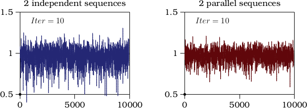
Figure 2: The variability of $\log(c_{n+1}/c_{n})$ plotted against $n$ for a simulation of $2$ chains and $10$ iterations per chain.

Increasing the number of walks per sequence to $100$ gives the results in figure 3. Both the bands are markedly narrower than in figure 2, and the values of $E$ confirm this, namely $0.06548$ for the left panel, and $0.0206$ for the panel on the right. This also supports a conclusion that the rate of convergence for Algorithm 2 is faster than that of Algoritm 1. Another example, in this case for $12$ sequences and $10^{4}$ started walks, are shown in figure 4, here the $E$ are $0.001951$ and $0.001091$, respectively, for the left and right panels.

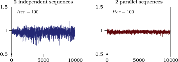
Figure 3: The variability of $\log(c_{n+1}/c_{n})$ plotted against $n$ for a simulation of $2$ chains and $100$ iterations per chain.

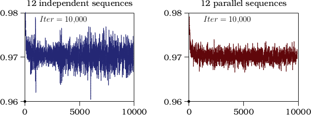
Figure 4: The variability of $\log(c_{n+1}/c_{n})$ plotted against $n$ for a simulation of $12$ chains and $10,\!000$ iterations per chain.

We have calculated $E$ for all our data and the results are shown in table 4. The notation is compacted so that $\overline{2}.1122\equiv 0.001122$ (that is, the barred digit is the number of zeros following the decimal point). Notice that Algorithm 2 consistently has smaller values for shorter runs, but that this advantage shrinks are longer simulations are done. By $10^{6}$ started walks, the widths are largerly the same. This suggest that the acceleration of convergence due to the parallel implementation in Algorithm 2 is best exploited by performing shorter simulations of the parallel implementation, and then to combine the results of several independent simulations for final results. In other words, more parallel sequences, rather than longer simulations, is the key to quick convergence and good results, and massively parallel implementations of Algorithm 2 may be the best approach.

Table 4: $E$ for Algorithms 1 and 2

	Algorithm 1					Algorithm 2
N	$N=1$	$N=2$	$N=3$	$N=6$	$N=12$	$N=2$	$N=3$	$N=6$	$N=12$
$1\;$	$0.2782$	$0.2578$	$0.2622$	$0.2708$	$0.2639$	$0.1886$	$0.1580$	$0.1113$	$\overline{1}.8023$
$10\;$	$0.1363$	$0.1129$	$0.1129$	$0.1129$	$\overline{1}.8501$	$\overline{1}.8186$	$\overline{1}.5643$	$\overline{1}.3870$	$\overline{1}.2556$
$10^{2}$	$\overline{1}.8394$	$\overline{1}.6548$	$\overline{1}.4348$	$\overline{1}.3292$	$\overline{1}.2388$	$\overline{1}.2060$	$\overline{1}.1754$	$\overline{1}.1284$	$\overline{2}.8540$
$10^{3}$	$\overline{1}.2783$	$\overline{1}.1103$	$\overline{1}.1077$	$\overline{1}.1112$	$\overline{2}.5158$	$\overline{2}.8695$	$\overline{2}.7670$	$\overline{2}.4156$	$\overline{2}.3038$
$10^{4}$	$\overline{2}.3329$	$\overline{2}.2493$	$\overline{2}.2130$	$\overline{2}.2903$	$\overline{2}.1951$	$\overline{2}.2811$	$\overline{2}.1979$	$\overline{2}.1551$	$\overline{2}.1091$
$10^{5}$	$\overline{2}.1244$	$\overline{3}.8238$	$\overline{3}.7084$	$\overline{3}.4961$	$\overline{3}.3755$	$\overline{3}.8673$	$\overline{3}.7317$	$\overline{3}.4936$	$\overline{3}.3511$
$10^{6}$	$\overline{3}.3980$	$\overline{3}.2771$	$\overline{3}.2294$	$\overline{3}.1590$	$\overline{3}.1125$	$\overline{3}.2742$	$\overline{3}.2262$	$\overline{3}.1575$	$\overline{3}.1120$
Notation: $\overline{a}.b_{1}b_{2}b_{3}b_{4}\equiv 0.b_{1}b_{2}b_{3}b_{4}\times 10^{-a}$

As a final test of our implementation we estimated the growth constants $\mu_{2}$ and $\mu_{3}$. In the square lattice we performed two simulation of walks of lengths up to $50,\!000$. The first simulation was stopped after a total of $105,\!685,\!556$ iterations (started walks) over $12$ parallel sequences (or about $8,\!807,\!130$ per parallel sequence), and the second was run to completion at $120,\!000,\!000$ iterations (started walks) over $12$ parallel sequence (or $10,\!000,\!000$ per parallel sequence). A three parameter fit of equation (16) to the weighted geometric average of the data for lengths $1\leq n\leq 50,\!000$ was used to determine an estimate of $\mu_{2}$. This shows that

$$\log\mu_{2}=0.970081152$$ (17)

compared to the estimate of $\log\mu_{2}=0.970081147258(8)$ by Clisby and Jensen [5], showing that our result is within $5\times 10^{-9}$ from their more accurate estimate. We do confirm the first 6 digits in the decimal expansion.

Next, we consider estimates of $\mu_{3}$ in the cubic lattice using more extensive simulations in order to both determine the efficiency of the algorithm, and to find good estimates of the growth constant.

In the cubic lattice we performed seven simulations of walks of lengths up to $50,\!000$ using Algorithm 2 with 12 parallel sequences, and discarded data for lengths over $49,\!900$ from our data due to boundary effects. The first simulation was of length $4,\!250,\!000$ iterations per parallel sequence (for a total of $51,\!000,\!000$ iterations), and the remaining six simulations were each of length $2,\!125,\!000$ iterations per parallel sequence (for a total of $25,\!500,\!000$ iterations for each simulation). These simulation give the $7$ estimates

$$\log\mu_{3}=\left\{\begin{array}[]{lll}1.5441604989&1.5441608584&1.5441603031\\ 1.5441607748&1.5441611068&1.5441612779\\ 1.5441608359\\ \end{array}\right.$$ (18)

each stated to 10 decimal places. A weighted average of these results give $\log\mu_{3}=1.544160769$. Rounding our result and comparing it to the best estimate by Clisby [3], namely $\log\mu_{3}=1.5441609707(58)$, show that we have verified six decimal places, namely

$$\log\mu_{3}=1.\underline{544160}77.$$ (19)

If, instead, the geometric averages over all the data in the seven simulations are taken, and then analysed, we obtain the estimate

$$\log\mu_{3}=1.54416076.$$ (20)

The total number of iterations, over all the simulations and sequences, is $204,\!000,\!000$.

The efficiency of algorithm 2 is best illustrated by performing shorter simulations, and comparing the results to the above. Simulations of walks to length $n=50,\!000$ were again performed, but now doing $200,\!000$ iterations per thread along $12$ sequences (for a total of $2,\!400,\!000$ per simulation - each of these simulation was just about $9.4$% of the length of those leading to the results in equation (18)). Over $31$ simulations we did a total of $74,\!400,\!000$ iterations. These simulations give the following results which are comparable in accuracy to the results in equation (18) and are

$$\log\mu_{3}=\left\{\begin{array}[]{llll}1.5441593027&1.5441599034&1.5441605413&1.5441604908\\ 1.5441611903&1.5441606073&1.5441603137&1.5441612410\\ 1.5441614305&1.5441604872&1.5441594056&1.5441608619\\ 1.5441599673&1.5441620647&1.5441622034&1.5441603728\\ 1.5441611795&1.5441607140&1.5441629101&1.5441609189\\ 1.5441591882&1.5441618451&1.5441618095&1.5441608069\\ 1.5441596354&1.5441606142&1.5441607758&1.5441595308\\ 1.5441597235&1.5441612369&1.5441619484\end{array}\right.$$ (21)

with results stated to 10 decimal places. Taking a simple average over these results gives $\log\mu_{3}=1.544160749$, showing that these data are converged. This result rounds to $1.54416075$ and is comparable to the result in equation (19). If the geometric average over all the data in the $31$ simulations are taken and then $\log\mu_{3}$ is computed, then the result is again

$$\log\mu_{3}=1.54416075,$$ (22)

as compared to equation (20).

The above results strongly suggest that shorter simulations using more sequences in parallel for longer walks give superior performance, at least when the aim is to estimate $\log\mu_{d}$ (our data also show that longer simulations are needed to get good results for the entropic exponent $\gamma$).

As a final test we sampled walks of length $n=200,\!000$. Nine simulations with $100,\!000$ started sequences per thread (for a total of $12\times 100,\!000=1,\!200,\!000$ iterations per simulation, or just half the number of started sequences per thread leading to the results in equation (21)) give the following estimates

$$\log\mu_{3}=\left\{\begin{array}[]{llll}1.5441618451&1.5441630316&1.5441630117\cr 1.5441625924&1.5441626936&1.5441623028\cr 1.5441628816&1.5441620305&1.5441633443\end{array}\right.$$ (23)

A simple average over the nine estimates gives $\log\mu_{3}=1.5441626371$. This slightly exceeds the better estimate in equation (22), but given that these simulations were very short (each taking an average of just 16.5 hours CPU time). The total number of iterations is $10,\!800,\!000$. Since these walks were also longer than those in equation (21), a better estimate of the exponent $\gamma$ is obtained, namely

$$\gamma=\left\{\begin{array}[]{llll}1.1608790435&1.1572583036&1.1613650153\cr 1.1543650430&1.1581152153&1.1578135872\cr 1.1576672680&1.1513397803&1.1561657305\end{array}\right.$$ (24)

Taking a simple average gives $\gamma=1.15722$, which compares well with the result in reference [15].

4 Conclusions

Our data clearly show that the parallel implementation of flatPERM using algorithm 2 (see figure 1) outperforms flatPERM as implemented using algorithm 1. Since algorithms 1 and 2 use the same computational resources (for example, CPU time and number of threads) our approach to analyse output in order to compare performance is a fair comparison to determine the relative improvement seen in algorithm 2 over algorithm 1.

The improvement seen in algorithm 2 is in particular evident by the reduction in the time it takes to see convergence after it is initialised. In addition, there is also a noticeable improvement with increasing the number of parallel sequences in algorithm 2. This is seen, for example, in table 3 where there is an improvement with increasing number of sequences for low numbers of iterations. Similar improvements are seen in tables 1 and 2. However, the reduction in noise with the increasing number in sequences, in particular for algorithm 2, as shown in figures 2, 3 and figure 4, is more dramatic, and this is confirmed by the data in table 4 showing that algorithm 2 outperforms algorithm 1 in particular when each parallel sequence is shorter than about $10^{4}$ iterations (started walks).

We also estimated the growth constant $\mu_{d}$ for walks using algorithm 2. Our best results are

$$\mu_{d}=\cases{2.6381585(1),&\hbox{if $d=2$};\cr 4.684039(1),&\hbox{if $d=3$},}$$ (25)

obtained by exponentiating the results in equations (17) and (20) and rounding it in $d=2$ to seven decimal places, and in $d=3$ to six decimal places. The result in $d=2$ is different by about $1\times 10^{-7}$ from the result in reference [5], and that in $d=3$ by less than $1\times 10^{-6}$ from the result in reference [3]; see equation (12). The simulations leading to the results in equation (18) were all done on a single DELL Optiplex Desktop workstation, and the results in equations (21) and (23) were obtained by submitting our programs to a Dell R340 node with 12 threads (and 6 cores).

Using our data leading to the estimates in equation (18) we also estimated the entropic exponent $\gamma$ (see equation (16)). This was done by using the three parameter model in equation (16) with a minimum cut-off $n_{min}$ for $n$ (that is, for $n\geq n_{min}$). By extrapolating the results against $n_{min}$ our best estimates are

$$\gamma=\cases{1.34416(42)&\hbox{if $d=2$};\cr 1.15643(55)&\hbox{if $d=3$}.}$$ (26)

If the analysis is done using the geometric average of the data instead, then the estimate $\gamma=1.15662$ is obtained instead in the cubic lattice.

If the analysis is repeated, but now using the best estimates for $\log\mu_{d}$ (equation (25)), then a two parameter fit using the model in equation (16) gives

$$\gamma=\cases{1.34319(56)&\hbox{if $d=2$};\cr 1.15681(17)&\hbox{if $d=3$}.}$$ (27)

These results should be compared to the exact value $\gamma=1.34375$ in two dimensions [6] and the estimate $\gamma=1.15698(34)$ [15] in three dimensions and are in both cases accurate to three decimal places (see also the estimate $1.15695300(95)$ [4] for a more accurate estimate in three dimensions). The differences from the exact value and the estimate in [15] are shown in brackets as an error term in equations (26) and (27).

The parallel implementation of PERM (using the flatPERM implementation of PERM) in this paper makes it possible to exploit the parallel architecture of modern computers by feeding a flatPERM-sequence to each thread. Each sequence is recursively evolved by the algorithm and the exchange of information between sequences occurs by the use of shared data which incorporates information about the ensemble landscape from the other sequences into a given sequence, thereby affecting its future evolution. This approach can be used in the same way to implement a parallel GARM algorithm (see reference [13]). Closer integration of communication between parallel sequences may also be imagined; for example, two sequences sampling walks in the square lattice may be considered as a single sequence sampling a path in the four dimensional hypercubic lattice. This approach may also give accelerated convergence but a parallel implementation may not be possible, as the four dimensional path will have to be sampled in a single thread.

We have also implemented an integrated parallel implementation of the Wang-Landau algorithm [18] using a set of interacting sequences on state space similar to algorithm 2. The Wang-Landau algorithm directly estimates the density of states by carrying out a random walk in energy space. It tracks the energy $E$ of a system: If the current energy $E_{old}$ ($g(E_{old})$) is the energy (respectively density) of the current configuration and $E_{new}$ ($g(E_{new})$) is the energy (respectively density) of the new proposed configuration, then the move is accepted with probability $p=\min\left\{\frac{g(E_{old})}{g(E_{new})},1\right\}$. Each time a state is visited by a sequence, the density of states is updated by a modification factor $f$ such that $g(E)\leftarrow g(E)\cdot f$. A histogram $H(E)$ of each visit is also kept and a flatness criterion for the histogram is used to update the modification factor $f$. That is, when the histogram achieves the flatness criterion it is reset and $f$ is reduced in a predetermined fashion. Care is usually taken here since if $f$ is decreased too rapidly this can lead to saturation errors (see reference [2]).

The parallel implementation for the Wang-Landau algorithm differs slightly from that of the PERM algorithm and an earlier approach of Zhan [19]. In our approach the parallel streams are used to control the update of a common $f$. The density of states for each stream are compared to estimate the error and then the updated $f$ value depends on this estimated error. That is, as the error declines the values of $f$ also decline. The standard observed relationship is that the statistical error scales proportionally with $\sqrt{\log{f}}$ (see reference [20]).

The benefit of dynamically adjusting the parameter $f$ is that the $f$ values decline rapidly when the algorithm is converging quickly and vice versa. In particular, as in the case of the PERM algorithm, we find that the initial rate of convergence is significantly accelerated. Previous works have suggested that in the absence of additional information, an optimal convergence rate might be achieved by decreasing $\log f$ at a rate of $1/t$ where $t$ is the normalized time of the simulation [21]. Moreover, numerical results suggest that this achieves a statistical error of $1/\sqrt{t}$ and, in general, a theoretical upper bound on the error behaviour was shown in reference [21] to be $1/t$. By taking advantage of the additional information provided by the communicating sequences in our algorithm, we report that for reasonable length simulations the estimates of $c_{n}$ are found to greater accuracy than those from independent parallel implementations of the standard $1/t$ algorithm.

Acknowledgements: EJJvR acknowledges financial support from NSERC (Canada) in the form of Discovery Grant RGPIN-2019-06303. SC acknowledges the support of NSERC (Canada) in the form of a Post Graduate Scholarship (Application No. PGSD3-535625-2019).

References

References

- [1] OpenMP API. https://www.openmp.org.
- [2] RE Belardinelli and VD Pereyra. Wang-Landau algorithm: A theoretical analysis of the saturation of the error. J Chem Phys, 127(18):184105, 2007.
- [3] N Clisby. Calculation of the connective constant for self-avoiding walks via the pivot algorithm. J Phys A: Math Theo, 46:245001, 2013.
- [4] N Clisby. Scale-free Monte Carlo method for calculating the critical exponent of self-avoiding walks. J Phys A: Math Theo, 50:264003, 2017.
- [5] N Clisby and I Jensen. A new transfer-matrix algorithm for exact enumerations: self-avoiding polygons on the square lattice. J Phys A: Math Theo, 45:115202, 2012.
- [6] B Duplantier. Polymer network of fixed topology: renormalization, exact critical exponent in two dimensions, and . Phys Rev Lett, 57:941–944, 1986.
- [7] SJ Fraser and MA Winnik. Variance reduction for lattice walks grown with markov chain sampling. J Chem Phys, 70:575–581, 1979.
- [8] P Grassberger. Pruned-enriched Rosenbluth method: simulations of polymers of chain length up to . Phys Rev E, 56:3682–3693, 1997.
- [9] JM Hammersley and KW Morton. Poor man’s Monte Carlo. J Roy Stat Soc Ser B (Meth), 16:23–38, 1954.
- [10] H Kesten. On the number of self-avoiding walks. J Math Phys, 4:960–969, 1963.
- [11] H Meirovitch. Computer simulation of the free energy of polymer chains with excluded volume and with finite interactions. Phys Rev A, 32:3709–3715, 1985.
- [12] T Prellberg and J Krawczyk. Flat histogram version of the pruned and enriched Rosenbluth method. Phys Rev Lett, 92:120602, 2004.
- [13] A Rechnitzer and EJ Janse van Rensburg. Generalized atmospheric Rosenbluth methods (GARM). J Phys A: Math Theo, 41:442002, 2008.
- [14] MN Rosenbluth and AW Rosenbluth. Monte Carlo calculation of the average extension of molecular chains. J Chem Phys, 23:356–359, 1955.
- [15] O Schramm. Conformally invariant scaling limits: an overview and a collection of problems. In Selected Works of Oded Schramm, pages 1161–1191. Springer, 2011.
- [16] MC Tesi, EJ Janse van Rensburg, E Orlandini, and SG Whittington. Monte Carlo study of the interacting self-avoiding walk model in three dimensions. J Stat Phys, 82:155–181, 1996.
- [17] FT Wall and JJ Erpenbeck. Statistical computation of radii of gyration and mean internal dimensions of polymer molecules. J Chem Phys, 30:637–641, 1959.
- [18] F Wang and DP Landau. Efficient, multiple-range random walk algorithm to calculate the density of states. Phys. Rev. Lett., 86:2050–2053, Mar 2001.
- [19] L Zhan. A parallel implementation of the Wang-Landau algorithm. Comp Phys Commun, 179(5):339–344, 2008.
- [20] C Zhou and RN Bhatt. Understanding and improving the Wang-Landau algorithm. Phys Rev E, 72(2):025701, 2005.
- [21] C Zhou and J Su. Optimal modification factor and convergence of the Wang-Landau algorithm. Phys Rev E, 78(4):046705, 2008.