DropCluster: A structured dropout for convolutional networks

Abstract

Dropout as a regularizer in deep neural networks has been less effective in convolutional layers than in fully connected layers. This is due to the fact that dropout drops features randomly. When features are spatially correlated as in the case of convolutional layers, information about the dropped pixels can still propagate to the next layers via neighboring pixels. In order to address this problem, more structured forms of dropout have been proposed. A drawback of these methods is that they do not adapt to the data. In this work, we introduce a novel structured regularization for convolutional layers, which we call DropCluster. Our regularizer relies on data-driven structure. It finds clusters of correlated features in convolutional layer outputs and drops the clusters randomly at each iteration. The clusters are learned and updated during model training so that they adapt both to the data and to the model weights. Our experiments on the ResNet-50 architecture demonstrate that our approach achieves better performance than DropBlock or other existing structured dropout variants. We also demonstrate the robustness of our approach when the size of training data is limited and when there is corruption in the data at test time.

1 Introduction

Convolutional neural networks (CNNs) have become a foundational tool for computer vision problems. Regularization is needed during CNN training to ensure that the model generalizes well to unseen data, especially when the training set is small, or the test set is noisy. Achieving good generalization is especially crucial for critical applications such as medical diagnostics, self-driving cars, or facial recognition.

Dropout is a well-known regularization approach to reduce generalization error (Srivastava et al., 2014). Dropout, which randomly drops units in hidden layers during each training iteration, can be interpreted as a way of ensembling thinned networks at test time. Although dropout has been successful for fully-connected layers, it has been less effective for CNNs. Recently, (Ghiasi et al., 2018) argued that the presence of spatial correlation between features in convolutional layers prevents the success of dropout.

In this work, we introduce a novel structured regularization for convolutional layers, called DropCluster, which learns the structure in feature maps and leverages this structure to drop features more effectively. Our method learns clusters in convolutional layer outputs during training. The clusters are learned after some number of epochs in training and updated at regular intervals for the rest of training. We drop features in two ways: first, we drop clusters of correlated features in each training step; second, if a channel does not demonstrate any clusterable structure, we drop that channel entirely.

The clustering algorithm we use is recursive nearest agglomeration (ReNA) (Hoyos-Idrobo et al., 2018). ReNA is well-suited to two-dimensional images because it assumes some prior graph structure connecting features which are likely to be correlated, and is appropriate for learning clusters during training due to its fast computation (Aydore et al., 2019). In our application, the graph structure is given by adjacent pixels in each feature map. Our experiments on CIFAR-100 and Tiny ImageNet with ResNet-50 architecture demonstrate that our approach performs better than the alternatives.

Typically, the performance of machine learning models is evaluated on a separate test dataset. It is assumed that the training data is representative of the unseen data. However, this is not necessarily true in real-world applications. It is possible to encounter new data from a distribution different than the distribution of the training data (Liu et al., 2018; Recht et al., 2018). Even when humans can barely notice the difference, this mismatch between training and new data distributions can produce incorrect scientific conclusions or let attackers fool machine learning systems by feeding manipulated input to the models (Hendrycks & Gimpel, 2016). Therefore, achieving robustness to small perturbations in the data is essential especially for applications such as spam filters, detecting diseases or discovering astronomical phenomena (Hendrycks & Dietterich, 2019; Hendrycks et al., 2018). In this work, without including adversarial training, we evaluate the robustness of our DropCluster to common corruptions in the data. We use noise and blur corruptions as also used by several studies to demonstrate the fragility of CNNs (Hosseini et al., 2017; Dodge & Karam, 2017). Our results show that our DropCluster is more robust to these corruptions compared to other structured regularizers.

Fitting deep learning models with many parameters can be even more challenging when the sample size of training data is small. This problem can occur in fields such as astronomy, genomics, chemistry and medical imaging where data acquisition is expensive (Fan & Li, 2006; Consortium et al., 2015). Therefore, it is important for a machine learning model to perform well when trained on data with small sample size. We provide performance comparisons between our approach and other approaches to evaluate robustness to small sample size. Our results show that DropCluster performs better than the others even when the size of training data is reduced.

2 Related work

In order to address the limitation of dropout in CNNs, structured variants of dropout such as DropBlock, SpatialDropout and StochasticDepth have been proposed. Among these, the most relevant work to ours is DropBlock. DropBlock randomly drops a small square region of a feature map to remove certain semantic information. DropBlock improves training of convolutional layers, where traditional dropout does not, because selecting contiguous blocks leverages the spatial correlation found in feature maps (Ghiasi et al., 2018). The intention is that information from dropped features cannot leak into training via the features’ correlated neighbors. However, the shape of the dropped region is constant. We provide analysis showing that the shapes of correlated regions in feature maps tend to vary between channels. Our algorithm uses these varying shapes directly, dropping exactly the features which are highly correlated with each other.

StochasticDepth is another regularization tool for CNNs (Huang et al., 2016). To address the redundancy between layers, StochasticDepth randomly removes a subset of layers during training while maintaining a full depth network at test time. In Tompson et al. (2015), the authors formulated another structured dropout method called SpatialDropout that randomly drops channels of the network. However, StochasticDepth and SpatialDropout only make use of correlation within layers and within channels, respectively. Furthermore, they are informed by the network architecture, and not by patterns observed during model training, unlike our approach.

These approaches, which were specifically designed for convolutional filters and common CNN architectures, improve generalization. Our algorithm goes a step beyond architecture-driven regularization with data-driven regularization. We demonstrate the appropriateness of our approach with cluster analysis, and we demonstrate its effectiveness with improved performance and robustness on benchmark datasets.

3 ReNA: Recursive Nearest Agglomeration

In this work, we use ReNA to compute clusters. Although our method is independent of the choice of clustering algorithm, we choose ReNA because it is fast enough to compute multiple times during training, and because its graph-based feature grouping is well suited to two-dimensional (and potentially three-dimensional) images and feature maps, which have a natural graph structure defined by adjacent pixels. In this section we provide some details of the ReNA algorithm as background.

ReNA is initialized by placing every feature (pixel) in its own cluster, and proceeds by greedily merging pairs of connected pixels whose values are consistently similar across examples. This process is repeated until reaching a pre-specified number of clusters. ReNA’s computation time is $\mathcal{O}(nm\log(m/k))$, where $m$ is the number of pixels in the feature map, $n$ is the number of examples, and $k$ is the number of clusters (Hoyos-Idrobo et al., 2018). We hold $n$ constant as the number of examples in a single mini-batch, and we hold $k$ constant as a tunable hyperparameter. More formally, let $\boldsymbol{\Phi}\in\mathbb{R}^{k\times m}$ represent a feature grouping matrix that represents the $k$ clusters of $m$ features such that

$$\boldsymbol{\Phi}=\left[\begin{array}[]{cccc}\alpha_{1}\cdots\alpha_{1}&0\cdots 0&\cdots&0\cdots 0\\ 0\cdots 0&\alpha_{2}\cdots\alpha_{2}&\cdots&0\cdots 0\\ \vdots&\vdots&\vdots&\vdots\\ 0\cdots 0&0\cdots 0&0\cdots 0&\alpha_{k}\cdots\alpha_{k}\end{array}\right]$$ (1)

with an appropriate permutation of the features. The $\alpha_{i}$ values are chosen so that $\boldsymbol{\Phi}$ is an orthonormal matrix. ReNA obtains this featuring grouping matrix by using neighborhood graphs based on local statistics of the image. The algorithm takes the data $\mathbf{X}\in\mathbb{R}^{m\times n}$ where $n$ is the number of samples and the regular square lattice represented by a binary adjacency matrix $\mathbf{G}\in\mathbb{R}^{m\times m}\in\left\{0,1\right\}$ as graph.

ReNA converges when the desired number of clusters are learned. However, when the data lack meaningful clusters, ReNA will fail to converge. We make use of this property of ReNA to identify channels in the network which are too noisy to contribute to the learning task. We show empirically that dropping these channels improves learning, and we compute cluster tendency statistics on the feature maps to demonstrate that the lack of structure is not an artifact of our selected clustering algorithm, but is an important property of CNN training.

4 Clusters in Convolutional Layers

In this section, we motivate our approach by providing evidence that convolutional layer feature maps exhibit cluster tendency. We demonstrate cluster tendency qualitatively by visualizing computed clusters, and quantitatively by computing clustering statistics. We reference the Hopkins statistic for computing the degree to which clusters exist in data, and we introduce a novel modification to make the statistic appropriate for spatial data, such as images.

We train a LeNet-5 model on the CIFAR-10 dataset, and a ResNet-50 model on the CIFAR-100 and Tiny ImageNet datasets. We compute clusters in each channel given a mini-batch of outputs from the first convolutional layer. It is important to note that as the size of the convolutional layer outputs gets smaller, it becomes more challenging to identify structure in the data. Therefore our algorithm implements clustering only after the first convolutional layer for the datasets used in this paper. We also note that clusters in each feature map change rapidly during the early stages of training. Therefore we do not attempt to learn clusters until the 50^th epoch.

4.1 Qualitative Approach

For visualization of computed clusters, we train LeNet-5 on CIFAR-10 and ResNet-50 on CIFAR-100. The LeNet-5 architecture is useful for analysis because the relatively large feature maps produced by its first convolutional layer contain recognizable features with obvious connections to the raw input image. Analysis of ResNet-50 demonstrates that the behavior observed in LeNet-5 persists in more modern CNN architectures.

For the LeNet-5 architecture trained on CIFAR-10, we compute clusters on the outputs of the first convolutional layer after training the model for 50 epochs. The third row in Figure 1 shows the clusters at each channel. It can be observed that channel 3 captures vertical features while channel 5 captures horizontal features. The correlated groups of features identified by clustering are not found in regular square blocks, which would be adequately regularized by a method such as DropBlock. Instead, they are irregularly shaped. Furthermore, we observed during our experiments that the structure of the clusters varies between training runs, due to random initialization of the model weights. Both of these observations point to the need for an adaptive, data-driven approach to regularizing convolutional layers.

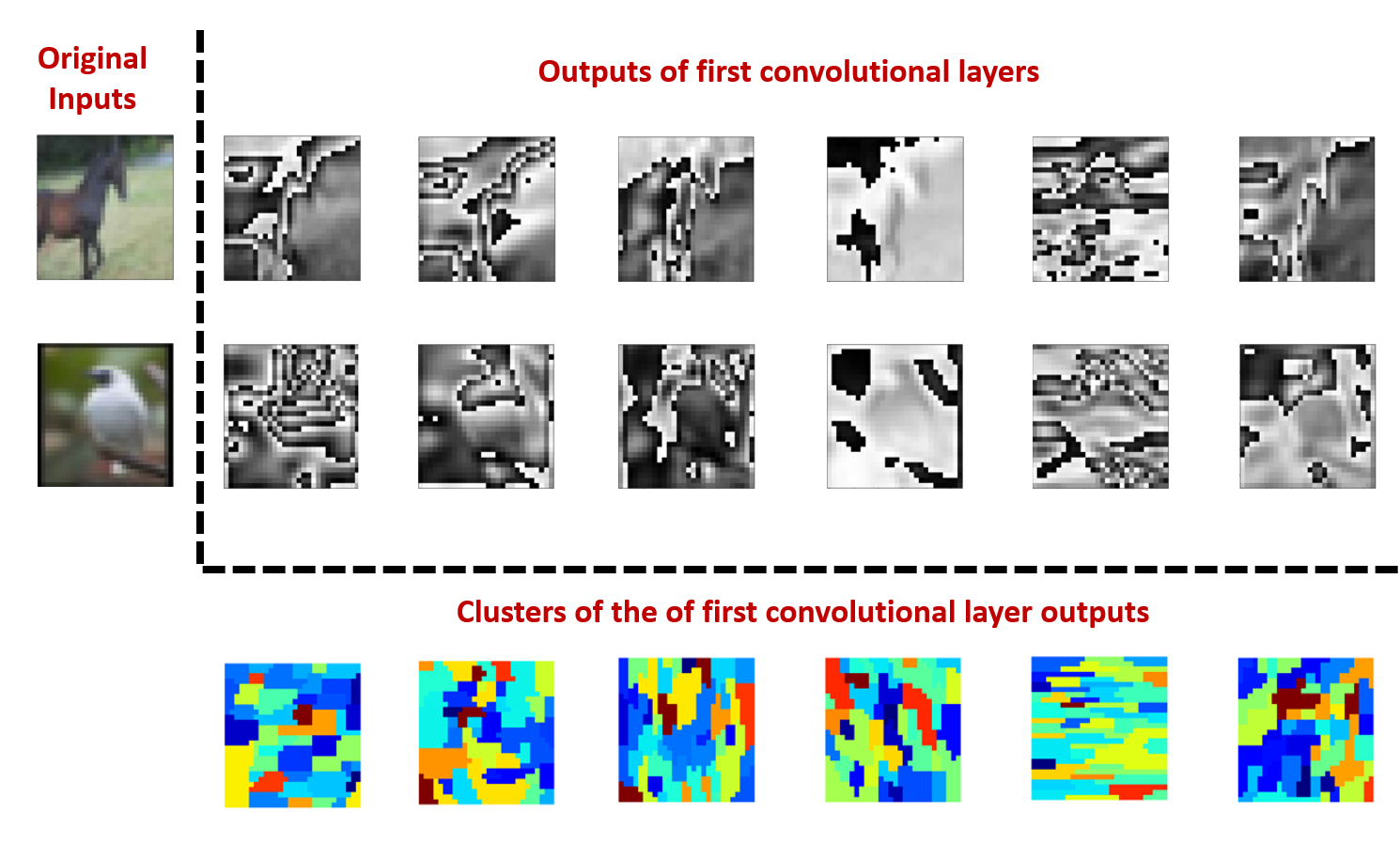
Figure 1: Clusters of the first convolutional layer outputs from a LeNet-5 model trained on the CIFAR-10 dataset after 50 epochs. This layer includes 6 channels. The left two images are the original input samples (horse and bird). The black-and-white images are the feature maps of these two samples at the first convolutional layer. The third row shows the clusters of these 6 channels.

Similarly, for ResNet-50 trained on CIFAR-100, we compute clusters on the outputs of the first convolutional layer after training the model for 50 epochs. This layer includes 64 channels. The output size of each channel is 16$\times$16 which is much smaller than the LeNet-5 outputs. For each channel, we compute 15 clusters. Figure 2 shows the clusters found in these 64 channels. Again, clusters are irregularly shaped, necessitating an adaptive regularization strategy.

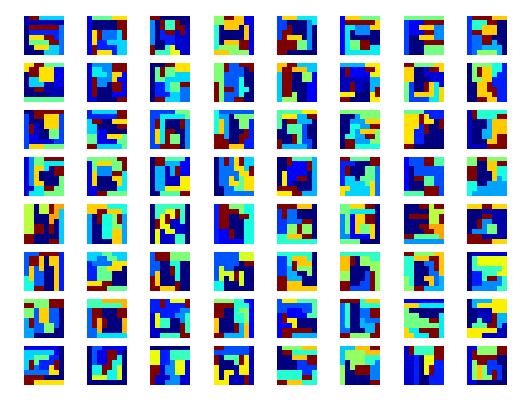
Figure 2: Clusters of the first convolutional layer outputs from a ResNet-50 model trained on the CIFAR-100 dataset.

Across many training runs, we found that training LeNet-5 on CIFAR-10 and ResNet-50 on CIFAR-100 did not result in any unstructured channels where features were not clusterable. However, unstructured channels were present when training ResNet-50 on Tiny ImageNet, where dropping unstructured channels improved performance. These unstructured channels are clearly visible in Figure 3. In channels $2,5,6,8,13,$ etc., ReNA was not able to converge, providing qualitative evidence of lack of structure. In the following section, we investigate this lack of structure more rigorously.

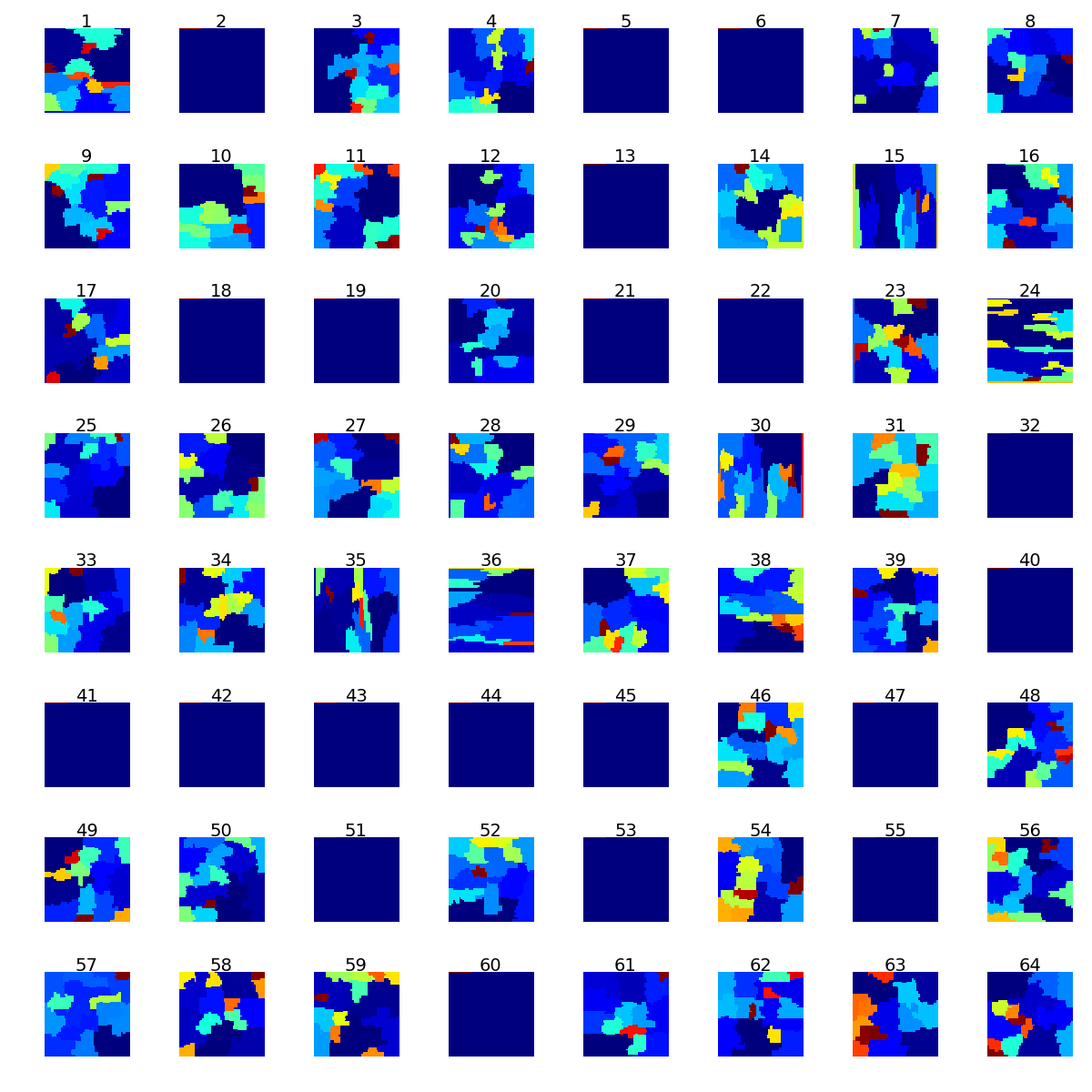
Figure 3: Clusters of the first convolutional layer outputs from a ResNet-50 model trained on the Tiny ImageNet dataset for $50$ epochs without any dropout. The channel indices are shown at the top of each image. The dark blue images represent the channels where ReNA was not able to compute the desired number of clusters ($15$ in this case). These channels also had cluster tendency values close to $0$.

4.2 Quantitative Approach: Spatial Clustering Statistics

In this section, we present quantitative evidence of the presence of clusters in feature maps, and of the variability of clusters between channels. We first discuss the Hopkins statistic (Banerjee & Dave, 2004), a measure used in clustering literature to quantify the presence of clusters in data. Then we propose a novel adaptation of the Hopkins statistic making it appropriate for image data.

The Hopkins statistic is a cluster tendency measure whose value is irrespective of any particular clustering algorithm. Computation of the Hopkins statistic begins by generating $m$ random points uniformly distributed between the minimum and maximum of each feature, and also sampling $m$ actual data points from the collection of $n$ data points $(m<<n)$. For both sets of points, it measures the distance to the nearest neighbor in the original dataset. For each sample $i$ in both sets, let $u_{i}$ be the nearest neighbor distance from the artificial points and $w_{i}$ be the nearest neighbor distance from the actual points. Then the Hopkins statistic is defined as

$$H=\frac{\sum_{i=1}^{m}u_{i}}{\sum_{i=1}^{m}u_{i}+\sum_{i=1}^{m}w_{i}}.$$ (2)

When the actual data points are approximately uniformly distributed, they will have similar distances to the randomly generated artificial points, and $H$ will be close to $0.5$, implying lack of cluster tendency. If, on the other hand, $H$ is close to $1$, then we can conclude that the data exhibits strong cluster tendency. Values of $H$ near $0$ implies the data are regularly spaced.

The Hopkins statistic is not applicable to image data because it does not take the ordering of features into account. Direct application to images would consider only the pixel intensities, and not their spatial locations. Therefore, we propose a new cluster tendency statistic Spatial Hopkins based on the difference of each pixel’s intensity from its neighbors. When there is spatial structure in the data, then each pixel’s intensity value will be close to its neighbors’ values. Based on this observation, we sample $m$ pixel locations $(x_{i},y_{i})$ uniformly randomly from $x_{i}\in\{2,\cdots,X-1\}$ and $y_{i}\in\{2,\cdots,Y-1\}$, $i\in 1,\cdots,m$ for an image $I$ of size $X\times Y$. We avoid pixels on the edges of the image for convenience. Similar to the Hopkins statistic, we choose $m<<XY$. Then we compute the average $L_{2}$ distance between the value of the pixel at this location and its $8$ neighbors as:

$$w_{i}=\frac{1}{8}\sum_{u,v}\|I(x_{i},y_{i})-I(u,v)\|_{2}$$ (3)

where $(u,v)\in\{(x_{i}-1,y_{i}-1),(x_{i}-1,y_{i}),(x_{i}-1,y_{i}+1),(x_{i},y_{i}-1),(x_{i},y_{i}+1),(x_{i}+1,y_{i}-1),(x_{i}+1,y_{i}),(x_{i}+1,y_{i}+1)\}$. Next, we sample another $m$ pixel locations, $(q_{1},r_{1}),\cdots,(q_{m},r_{m})$ again uniformly randomly in the image, and compute average distance between the intensities of $(x_{i},y_{i})$ and the neighbors of $(q_{i},r_{i})$:

$$z_{i}=\frac{1}{8}\sum_{u,v}\|I(q_{i},r_{i})-I(u,v)\|_{2}.$$ (4)

The set of points ${(u,v)}$ are the neighbors of $(x_{i},y_{i})$ in both equations. Finally, similar to the Hopkins statistic, we compute our Spatial Hopkins metric for a given image as:

$$S=\frac{\sum_{i=1}^{m}z_{i}}{\sum_{i=1}^{m}z_{i}+\sum_{i=1}^{m}w_{i}}.$$ (5)

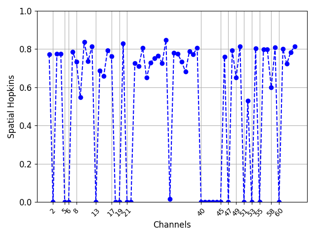
Figure 4: Spatial Hopkins statistic as a measure of cluster tendency for the first convolutional layer outputs from a ResNet-50 model trained on the Tiny ImageNet dataset for $50$ epochs without any dropout.

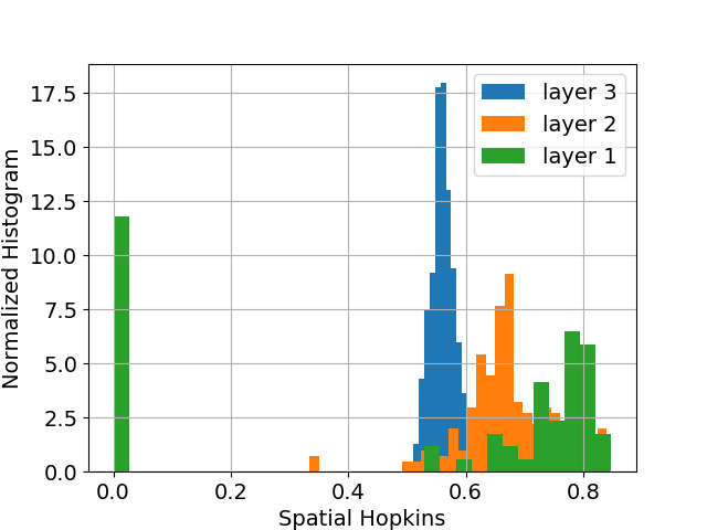
Figure 8: Histograms of Spatial Hopkins values from different layers. As the layer gets deeper, the center of histograms approach $0.5$ indicating less structure.

As is the case with the original Hopkins statistic, the Spatial Hopkins statistic will have values near $0.5$ if the data have no clustered structure. In Figure 4, we report the average Spatial Hopkins values across a mini-batch for each channel from the outputs of the first convolutional layer of Tiny ImageNet with a ResNet-50 model trained for $50$ epochs. It can be seen that the majority of the channels have Spatial Hopkins values close to $1$ indicating the presence of structure. In these channels, we cluster features and drop one cluster at a time. However, for channels such as $2,5,6,8,13,$ etc. the values are close to $0$, indicating a lack of structure. These correspond to the channels in Figure 3 where ReNA was not able to find any clusters. We set these channels’ output to zero in training and at test time. In Figure 8, we report the histogram of Spatial Hopkins values for deeper layers where it can be seen that the values tend toward $0.5$ for deeper layers. We advise practitioners to inspect these histograms to decide at which layer to implement DropCluster.

The variability in cluster shapes found in feature maps, and the variability in cluster tendency between structured and unstructured channels, demonstrate the need for data-driven regularization in CNN model training. Our algorithm’s ability to adapt to these sources of variability explains its improved performance.

Algorithm 1 Compute Clusters

Input:

$\mathbf{A}\in\mathbb{R}^{b\times t\times w\times h}$, output activations of the first convolution layer, where $b$ is the mini-batch size, $t$ is the number of channels and $w\times h$ is the size of feature map at each channel.

$n$, number of clusters to compute

Output:

$\mathbf{T}\in\{0,1\}^{t\times n\times w\times h}$, cluster assignments for each pixel in each channel, where $1$ indicates membership.

$\mathbf{N}$, set of indices of unstructured channels

1:  for $i=1$ to $t$ do

2:     Train ReNA on channel $i$: rena.fit$(A[:,i,:,:])$

3:     Let $m$ be the number of clusters found by ReNA

4:     if $m>n$ then

5:        Append $i$ to $\mathbf{N}$

6:     else

7:        {Record cluster indices}

8:        Let $\mathbf{T}=$ rena.get_clusters$()$

9:     end if

10:  end for

11:  Return $\mathbf{T}$, $\mathbf{N}$

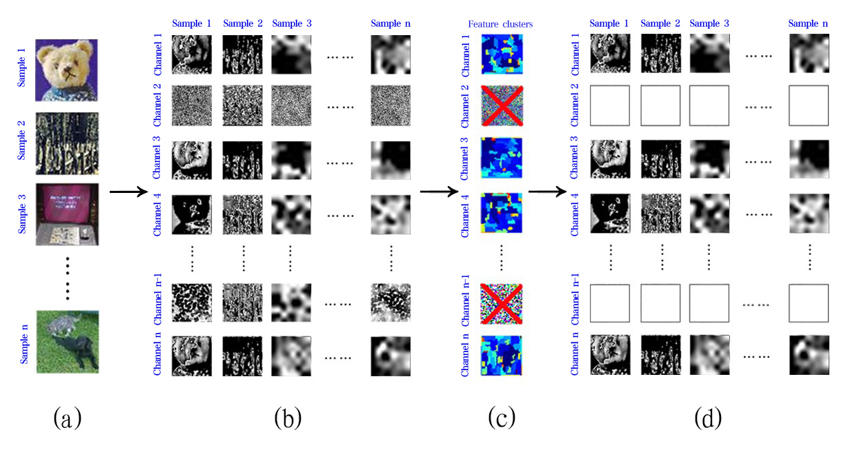
Figure 5: Illustration of dropping unstructured channels (a) Input image mini-batch to a CNN. (b) Output activations of a convolutional layer with several channels. (c) Feature clusters for each channel generated by ReNA. Channels that do not contain the desired number of clusters are identified as unstructured channels (marked with red X). (d) Inputs to the next layer after dropping unstructured channels.

5 DropCluster

In this section, we introduce our novel regularizer DropCluster. Our approach consists of two steps: (i) computing clusters in feature maps and identifying unstructured channels which are not clusterable, (ii) dropping random clusters from the structured channels during training and masking all unstructured channels both during training and inference.

First, we apply ReNA to extract clusters from the outputs of the first convolutional layer. Since structure in convolutional layers tends to change rapidly near the beginning of training, we apply this step after some fixed number of epochs, say $s$, in training and update it every $s$ epochs. We found $s=50$ to be a suitable choice, and we use it in all experiments in this paper. We use the publicly available implementation for ReNA (Idrobo, 2017) with the maximum number of iterations set to $1000$ and the graph structure defined by adjacency, where each pixel has connections to the four pixels above, below, left, and right. The clustering steps are explained in detail in Algorithm 1. Figure 5 illustrates dropping the unstructured channels.

Second, we drop randomly selected clusters from structured channels during training only, and mask unstructured channels during training and inference. Similar to standard dropout, we do not drop clusters in the structured channels during inference. But channels which are found to have no cluster structure stay masked in both training and inference, similar to channel pruning (He et al., 2017). The details of how clusters are dropped and channels are masked are given in Algorithm 2 and also illustrated in Figure 6.

Algorithm 2 Apply DropCluster

Input:

$\mathbf{A}\in\mathbb{R}^{b\times t\times w\times h}$, output activations of the first convolution layer, where $b$ is the mini-batch size, $t$ is the number of channels and $w\times h$ is the size of feature map at each channel.

$\mathbf{T}\in\{0,1\}^{t\times n\times w\times h}$, cluster assignments for each pixel in each channel

$\mathbf{N}$, the set of unstructured channel indices

$p$, the dropout probability

$n$, the number of clusters

Output:

$\mathbf{A}$, the masked outputs

1:  Initialize mask matrix to ones: $\mathbf{M}=\mathbf{1}_{t\times w\times h}$

2:  for $i=1$ to $t$ do

3:     if $i\in\mathbf{N}$ then

4:        Mask the entire channel: $\mathbf{M}[i,:,:]=\mathbf{0}_{w\times h}$

5:     else if $mode==Training$ then

6:        Randomly sample a set of cluster indices $\mathbf{L}\subset\{1,\cdots n\},|\mathbf{L}|=\lfloor pn\rfloor$

7:        for $l$ in $\mathbf{L}$ do

8:           $\mathbf{M}[i,:,:]\leftarrow\mathbf{M}\times(1-\mathbf{T}[i,l,:,:])$

9:        end for

10:     end if

11:  end for

12:  Repeat the mask along mini-batch dimension: $\mathbf{M}\leftarrow\mathbf{M}.repeat(b,1,1,1)$

13:  Apply the mask: $\mathbf{A}\leftarrow\mathbf{A}\times\mathbf{M}$

14:  Normalize the features: $\mathbf{A}\leftarrow\mathbf{A}\times\mbox{count}(M)/\mbox{count\_ones}(M)$

15:  return $\mathbf{A}$

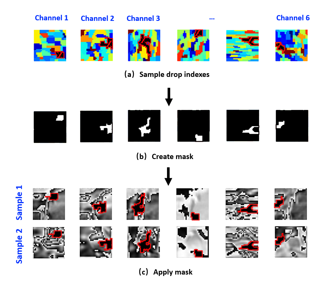
Figure 6: Visualization of dropping a single cluster from structured channels detailed in Algorithm 2. In practice, we drop more than a single cluster.

6 Experiments

In this section, we empirically evaluate the effectiveness of our DropCluster for image classification tasks. We compare our approach with dropout, DropBlock, SpatialDropout, StochasticDepth, and training without any type of dropout. We show that DropCluster achieves better Top1 (%) accuracy than other regularizers on both CIFAR-100 and Tiny ImageNet, and better Top5 (%) accuracy on CIFAR-100.

The goal of regularization is to improve how the model generalizes to unseen data. Two important problems in generalization are small sample sizes available at training time, and test data that comes from a different distribution than the training data. In order to study robustness to small sample size in training and corrupted test data, we supplement our standard benchmark results with experiments on various sample sizes and with noise and blur corruptions.

Implementation Details:

We use the standard widely used CNN architecture ResNet-50 (He et al., 2016) in all our experiments, changing only the types of dropout. We vary the dropout probability parameter $p$ for all dropout models for CIFAR-100 from $0.1$ to $0.3$ with a grid of $0.05$ and for Tiny ImageNet from $0.1$ to $0.5$ with a grid of $0.1$. We use the momentum SGD algorithm (Sutskever et al., 2013) with initial learning rate $0.1$ and momentum parameter $0.9$ for training. A scheduler is used with a multiplicative factor of learning rate decay $0.1$ applied at epochs $150$ and $200$. The weight decay parameter for CIFAR-100 is set to $5e-4$ and to $1e-4$ for Tiny ImageNet. We repeat each experiment for $4$ different random initializations. We report the average accuracy of predictions on the test set computed after each of the last $50$ epochs of training, averaged over $4$ random initializations.

The dropout and SpatialDropout regularizers are implemented by inserting the corresponding dropout layer with a dropout rate $p$ after the convolutional layer in the fourth group of ResNet blocks in both CIFAR-100 and Tiny ImageNet. Following the publicly available implementation of DropBlock (Ramos, 2019), we use a block size of $5\times 5$ for CIFAR-100 and $7\times 7$ for Tiny ImageNet in all experiments with DropBlock. We follow Ghiasi et al. (2018) to match up the effective dropout rate of DropBlock to the desired dropout rate $p$. A DropBlock layer is applied after the fourth group in Tiny ImageNet and first group CIFAR-100. In (Ghiasi et al., 2018), DropBlock is applied to the fourth layer only, as well as to the third and fourth layers for ImageNet. In our experiments, applying it to the fourth layer only performed best so we report those results. For the StochasticDepth regularizer, we follow the method from Zhang et al. (2019) that randomly drops out entire ResNet blocks at a dropout rate $p$ during training.

We implement DropCluster only after the first convolutional layer and before the first group of ResNet blocks. The size of the channels become too small to exhibit any structure information in the subsequent layers. We do not apply DropCluster until $50^{th}$ ($s$ in Section section 5) epoch in training since the structure information can be highly variable at the beginning of training. At every $50$ epochs in training, we compute the clusters in structured channels and identify unstructured channels. We drop the unstructured channels entirely both in training and inference, and we drop random clusters from structured channels in training only, selecting new clusters at each mini-batch. That is, we apply Algorithm 1 at epochs $50,100,\cdots$, and we apply Algorithm 2 for each mini-batch. The number of clusters, $n$, is set to $15$.

Computational details:

We use Python 3.6 for implementation (Oliphant, 2007) using open-source libraries PyTorch (Paszke et al., 2019), scikit-learn (Pedregosa et al., 2011), and NumPy (Walt et al., 2011). Experiments are run using 8 Nvidia RTX 2080 Ti GPUs with 512 GB memory. Our implementation will be openly available upon acceptance and is provided in the supplementary material.

6.1 CIFAR-100 Image Classification

The CIFAR-100 dataset consists of $32\times 32$ RGB images from $100$ classes (Krizhevsky et al., 2009). For each class, there are $600$ different images. The standard split contains $50,000$ training images and $10,000$ test images. For each training sample, we apply horizontal random flipping, random rotation, $32\times 32$ random crops after padding with 4 pixels on each side and normalization following the common practice (Huang et al., 2016). For test samples, we only apply normalization as a pre-processing step.

Model	Dropout Probability	Top1 (%)	Top5 (%)
No Dropout	0	60.82	83.66
Dropout	0.2	61.00	84.32
DropBlock	0.15	62.01	84.54
DropCluster	0.1	63.01	85.45
SpatialDropout	0.15	61.04	84.63
StochasticDepth	0.25	61.73	85.39

Table 1: Average accuracy of predictions on the CIFAR-100 test set computed after each of the last $50$ epochs of training, averaged over $4$ random initializations, when full training set is used. Except for the model trained without dropout, we report the best result with best dropout probability for each model.

Standard Settings:

In this experiment, we use the full training data for training and uncorrupted test data for evaluation. We report Top1 (%) and Top5 (%) accuracy results on test data when the full training set is used for all models in Table 1. For each regularizer, we report the best result among the range of dropout probability values. The results show that DropCluster achieves the highest performance among all regularizers both for Top1 (%) and Top5 (%) accuracies.

Small-sample Settings:

In this experiment, we explore the robustness of DropCluster to small sample sizes on CIFAR-100. For this purpose, we gradually reduce the size of the training dataset from $100\%$ to $20\%$ of the the full training size. Since DropBlock, DropCluster and StochasticDepth were the top $3$ performers when the full training set is used, we only compare these $3$ for the experiments in the small-sample setting. The results are summarized in Table 2. It can be seen that DropCluster stays more robust compared to DropBlock and StochasticDepth as the training set size decreases.

Model	DropBlock		DropCluster		StochasticDepth
Trainset size	Top1 (%)	Top5 (%)	Top1 (%)	Top5 (%)	Top1 (%)	Top5 (%)
100%	62.01	84.54	63.01	85.45	61.73	85.39
90%	61.89	85.07	62.31	85.01	56.30	82.11
80%	60.72	84.63	62.18	85.31	49.48	76.73
50%	61.39	85.84	61.36	85.69	42.16	70.81
20%	53.33	81.91	56.03	83.52	29.57	58.21

Table 2: Performance of DropBlock, DropCluster and StochasticDepth on test data of CIFAR-100 versus the training set size in %.

6.2 Tiny ImageNet (Tiny200) Classification

Tiny ImageNet dataset (CS231N, 2017) is a modified version of the original ImageNet dataset (Deng et al., 2009) containing $110,000$ images from $200$ classes with resolution $64\times 64$. We follow the standard $100,000$/$10,000$ training/validation split. We used horizontal random flip, scale, random crop and normalization for training images as in (Szegedy et al., 2015; Huang et al., 2017). During testing, we only apply a single crop and normalization. Following the common practice, we report the accuracy results on the validation set.

Standard Settings:

Similar to CIFAR-100, we first evaluate the performance of different dropout approaches trained on the full training dataset. In Table 3, we compare the performance of each model for the Tiny ImageNet dataset on uncorrupted validation data. The results show that our DropCluster performs the best for Top1 (%) accuracy. However, StochasticDepth performs better than DropCluster for Top5 (%) accuracy.

Model	Dropout Probability	Top1 (%)	Top5 (%)
No Dropout	0	64.69	83.49
Dropout	0.4	64.93	84.49
DropBlock	0.1	65.59	84.14
DropCluster	0.1	66.26	84.35
SpatialDropout	0.1	64.85	84.13
StochasticDepth	0.1	64.86	85.41

Table 3: Average accuracy of predictions on the Tiny ImageNet test set computed after each of the last $50$ epochs of training, averaged over $4$ random initializations, when full training set is used. Except for the model trained without dropout, we report the best result with best dropout probability for each model.

Small-sample Settings:

Similar to the experiments on the CIFAR-100 dataset, we explore the robustness of DropCluster, DropBlock and StochasticDepth to small training datasets. We summarize the results in Table 4. The results demonstrate that DropCluster is more robust than DropBlock to reduced sample size as measured by Top1 % accuracy. StochasticDepth performs better than DropCluster in Top1 % when the training size is $70\%$ and $50\%$.

Model	DropBlock		DropCluster		StochasticDepth
Trainset size	Top1 (%)	Top5 (%)	Top1 (%)	Top5 (%)	Top1 (%)	Top5 (%)
100%	65.59	84.14	66.26	85.35	64.86	85.41
90%	64.49	84.67	65.16	85.03	63.59	83.74
70%	61.89	82.70	62.29	82.88	62.52	83.23
50%	56.88	78.99	57.92	79.83	58.86	80.38
30%	48.42	72.03	49.18	72.65	48.97	72.26
10%	28.89	52.10	29.04	52.77	26.29	49.97

Table 4: Performance of DropBlock, DropCluster and StochasticDepth on Tiny ImageNet versus the training set size in % .

Corruption Settings:

In order to evaluate the robustness of DropCluster and other approaches to corruption in test data, we generated corrupted test datasets using the implementation provided by Hendrycks & Dietterich (2019). We use $7$ different types of corruption: Gaussian noise, shot noise, impulse noise, defocus blur, glass blur, motion blur and zoom blur using various severity levels as described in (Hendrycks & Dietterich, 2019). Figure 7 shows the effects of these corruptions on a sample image.

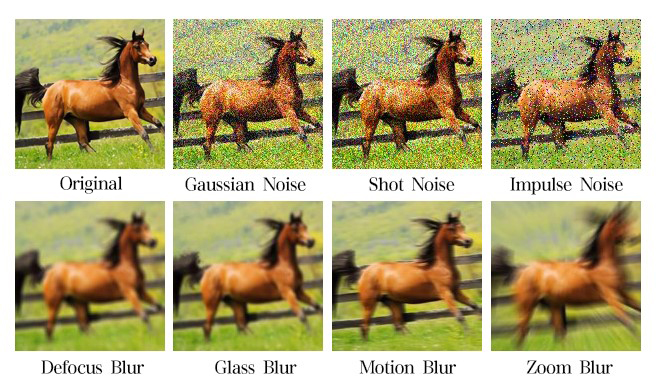
Figure 7: A sample image with different noise and blur corruptions.

We report the performance of DropBlock, DropCluster and StochasticDepth under common noise and blur corruptions with severity level 1 in Table 5. We also show the performance as a function of more severity levels in Figures 9 and 10. These results demonstrate that our DropCluster is more robust to corruption than DropBlock and StochasticDepth.

Model	DropBlock		DropCluster		StochasticDepth
CORRUPTION	Top1 (%)	Top5 (%)	Top1 (%)	Top5 (%)	Top1 (%)	Top5 (%)
GAUSSIAN	61.25	82.53	62.57	83.31	62.08	82.58
SHOT	60.57	82.46	61.92	82.79	61.64	82.00
IMPULSE	58.31	79.97	58.85	80.34	57.83	79.23
DEFOCUS	54.48	76.68	56.29	78.94	52.40	74.56
GLASS	48.87	72.44	51.94	75.23	47.92	70.60
MOTION	56.27	78.85	58.44	79.92	57.45	78.97
ZOOM	51.63	74.51	54.07	76.72	50.18	72.99

Table 5: Performance of DropBlock, DropCluster and StochasticDepth on validation data of Tiny ImageNet versus common noise and blur corruptions with severity level 1.

7 Conclusion

In this work, we propose a new data-driven regularizer DropCluster for CNNs. Our approach is based on learning correlated and redundant information in the data by using a clustering algorithm. DropCluster drops spatially correlated features in structured and all features in unstructured feature maps. We also propose a Spatial Hopkins statistic to evaluate cluster tendency. Our statistic does not depend on the clustering algorithm or the number of clusters. We show that convolutional layers exhibit cluster tendency via our Spatial Hopkins statistic and visual inspection. Our results on CIFAR-100 and Tiny ImageNet demonstrate that our approach performs better than the alternatives and is more robust to small-sample size of training data and corruption in new data. Our findings indicate that the structure in convolutional layers can be leveraged for training CNNs to achieve better performance and robustness.

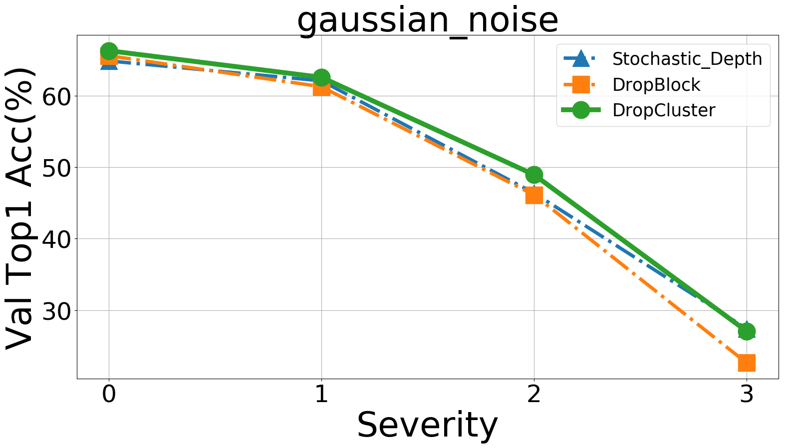
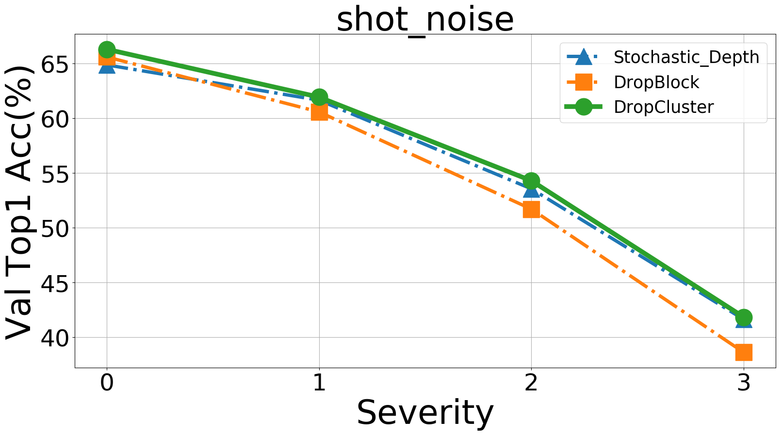
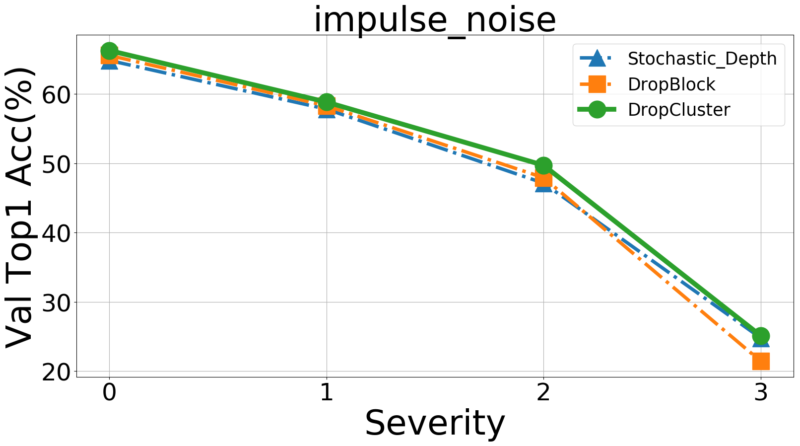
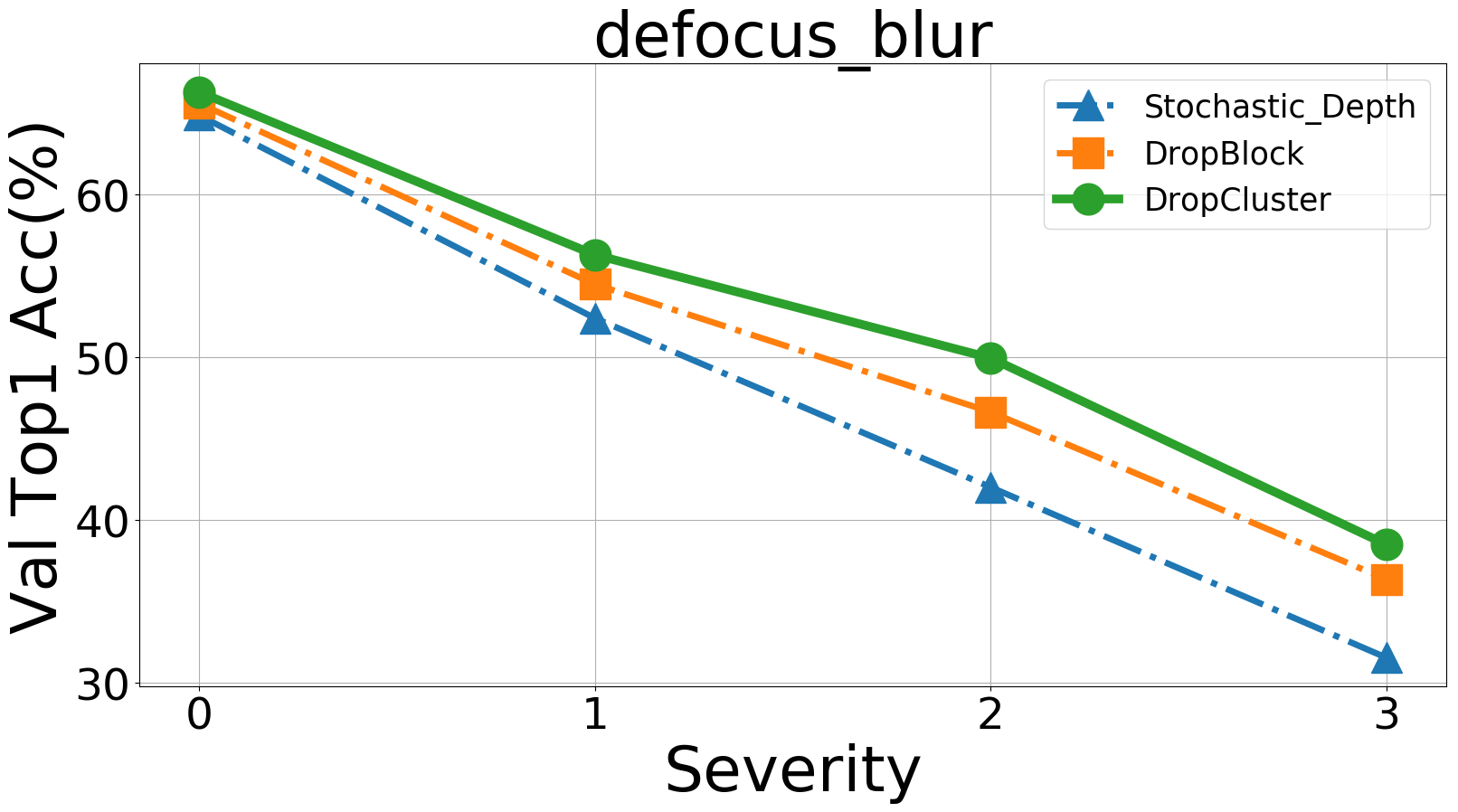
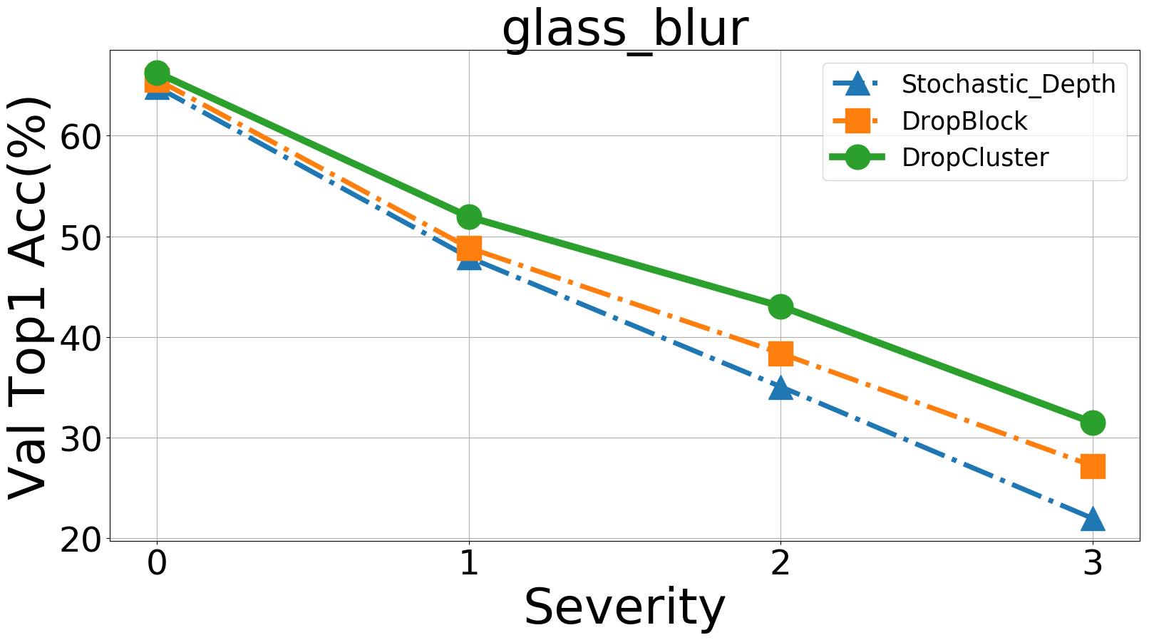
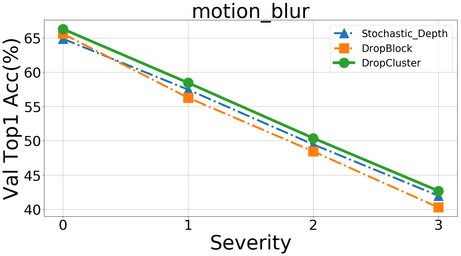
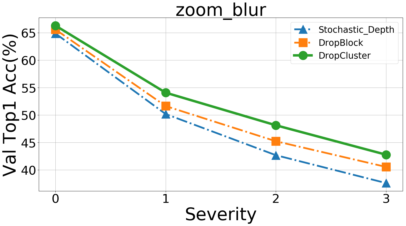
Figure 9: Top1 % performance of different dropout models on validation data of Tiny ImageNet versus severity levels in corruption.

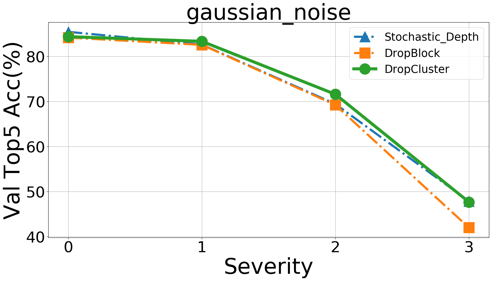
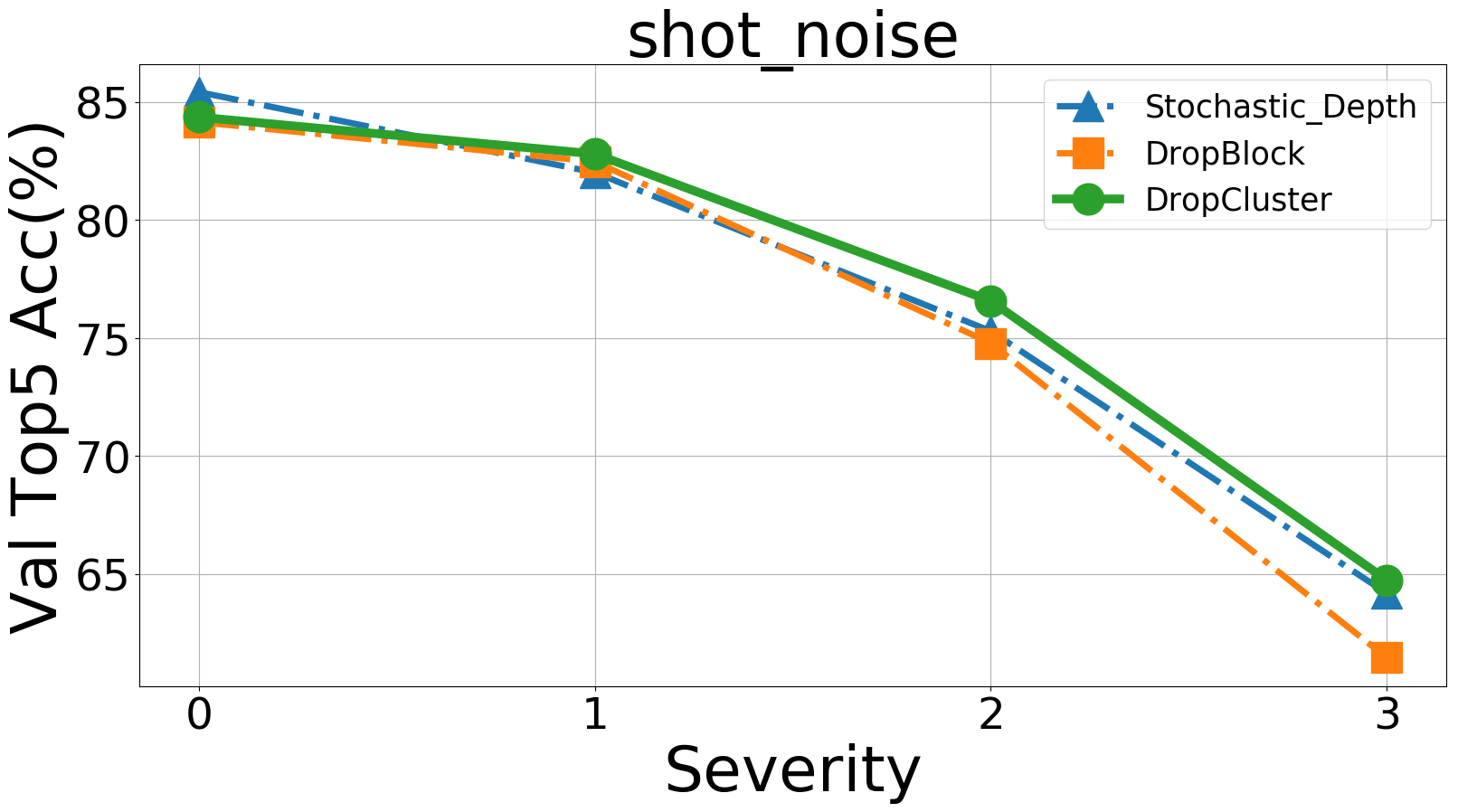
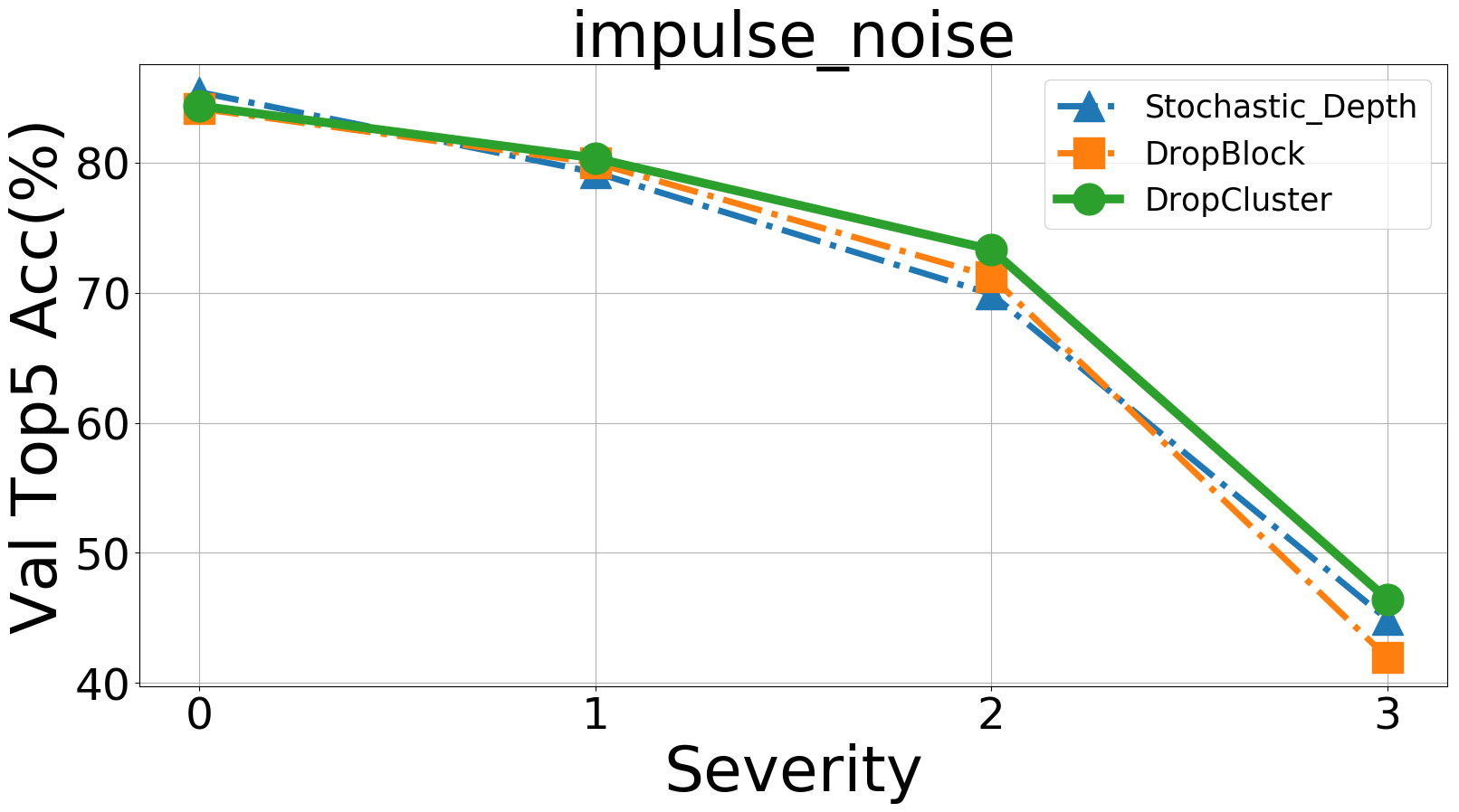
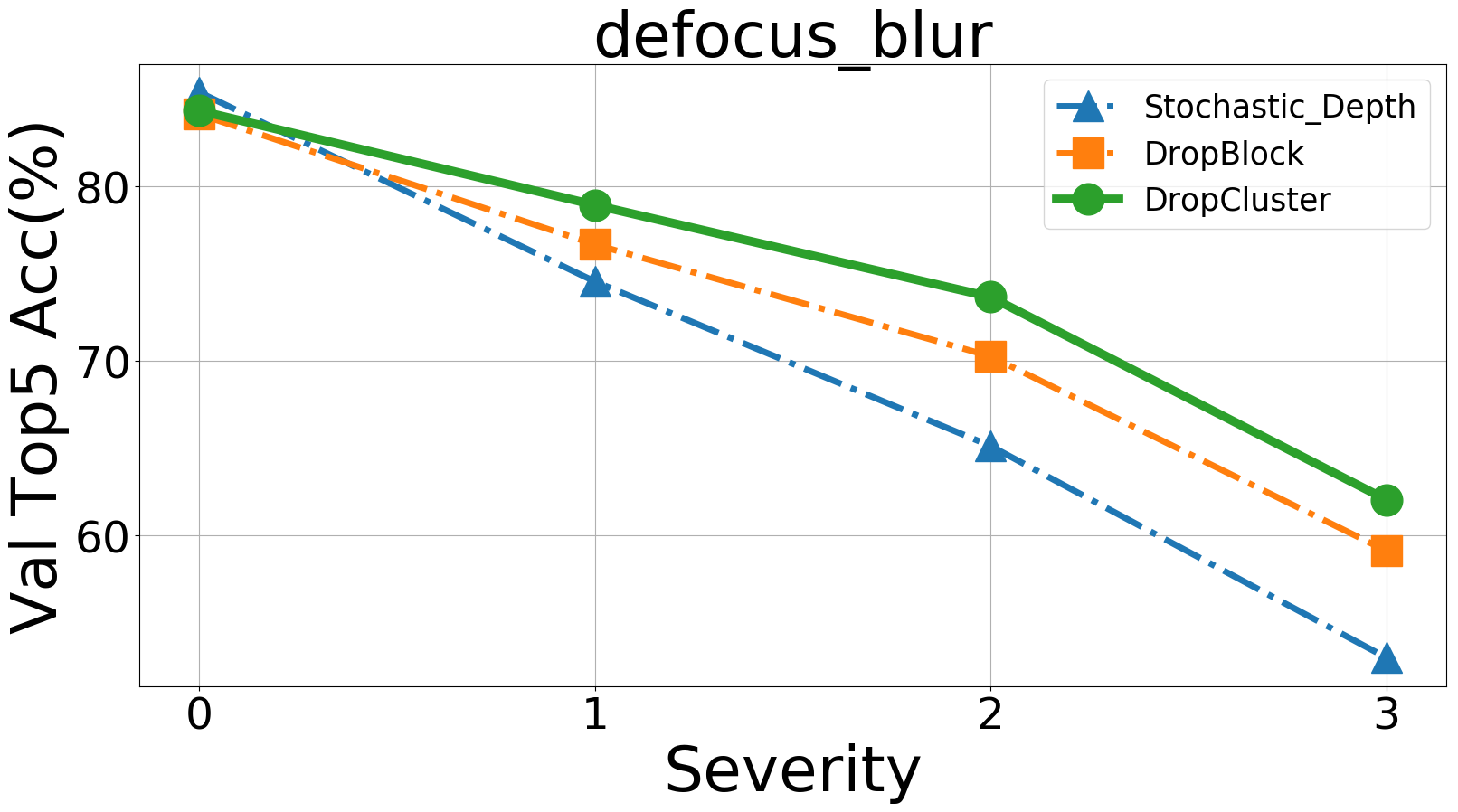
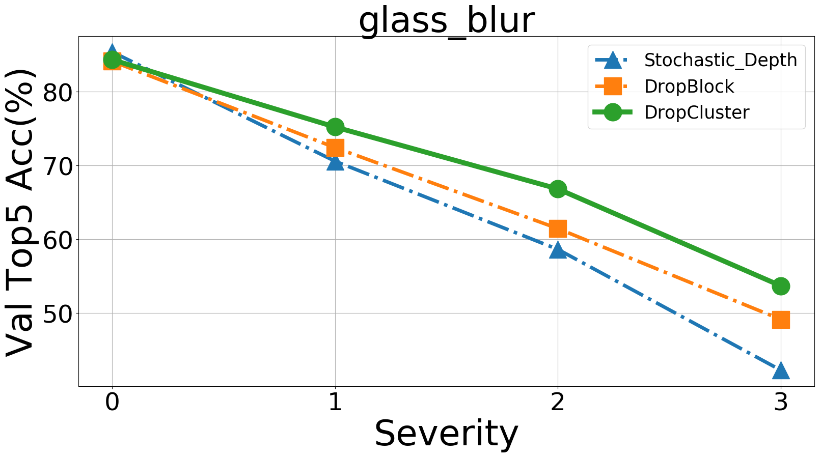
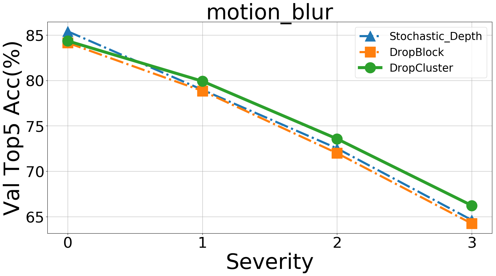
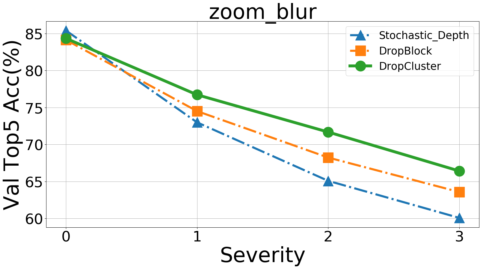
Figure 10: Top5 % performance of different dropout models on validation data of Tiny ImageNet versus severity levels in corruption.

References

- Aydore et al. (2019) Aydore, S., Thirion, B., and Varoquaux, G. Feature grouping as a stochastic regularizer for high-dimensional structured data. In International Conference on Machine Learning, pp. 385–394, 2019.
- Banerjee & Dave (2004) Banerjee, A. and Dave, R. N. Validating clusters using the hopkins statistic. In 2004 IEEE International conference on fuzzy systems (IEEE Cat. No. 04CH37542), volume 1, pp. 149–153. IEEE, 2004.
- Consortium et al. (2015) Consortium, . G. P. et al. A global reference for human genetic variation. Nature, 526(7571):68–74, 2015.
- CS231N (2017) CS231N, S. Tiny ImageNet Visual Recognition Challenge. https://tiny-imagenet.herokuapp.com/, 2017. [Online; accessed February 2020].
- Deng et al. (2009) Deng, J., Dong, W., Socher, R., Li, L.-J., Li, K., and Fei-Fei, L. Imagenet: A large-scale hierarchical image database. In 2009 IEEE conference on computer vision and pattern recognition, pp. 248–255. Ieee, 2009.
- Dodge & Karam (2017) Dodge, S. and Karam, L. A study and comparison of human and deep learning recognition performance under visual distortions. In 2017 26th international conference on computer communication and networks (ICCCN), pp. 1–7. IEEE, 2017.
- Fan & Li (2006) Fan, J. and Li, R. Statistical challenges with high dimensionality: Feature selection in knowledge discovery. arXiv preprint math/0602133, 2006.
- Ghiasi et al. (2018) Ghiasi, G., Lin, T.-Y., and Le, Q. V. Dropblock: A regularization method for convolutional networks. In Advances in Neural Information Processing Systems, pp. 10727–10737, 2018.
- He et al. (2016) He, K., Zhang, X., Ren, S., and Sun, J. Identity mappings in deep residual networks. In European conference on computer vision, pp. 630–645. Springer, 2016.
- He et al. (2017) He, Y., Zhang, X., and Sun, J. Channel pruning for accelerating very deep neural networks. In Proceedings of the IEEE International Conference on Computer Vision, pp. 1389–1397, 2017.
- Hendrycks & Dietterich (2019) Hendrycks, D. and Dietterich, T. Benchmarking neural network robustness to common corruptions and perturbations. arXiv preprint arXiv:1903.12261, 2019.
- Hendrycks & Gimpel (2016) Hendrycks, D. and Gimpel, K. Early methods for detecting adversarial images. arXiv preprint arXiv:1608.00530, 2016.
- Hendrycks et al. (2018) Hendrycks, D., Mazeika, M., and Dietterich, T. Deep anomaly detection with outlier exposure. arXiv preprint arXiv:1812.04606, 2018.
- Hosseini et al. (2017) Hosseini, H., Xiao, B., and Poovendran, R. Google’s cloud vision api is not robust to noise. In 2017 16th IEEE International Conference on Machine Learning and Applications (ICMLA), pp. 101–105. IEEE, 2017.
- Hoyos-Idrobo et al. (2018) Hoyos-Idrobo, A., Varoquaux, G., Kahn, J., and Thirion, B. Recursive nearest agglomeration (rena): fast clustering for approximation of structured signals. IEEE transactions on pattern analysis and machine intelligence, 41(3):669–681, 2018.
- Huang et al. (2016) Huang, G., Sun, Y., Liu, Z., Sedra, D., and Weinberger, K. Q. Deep networks with stochastic depth. In European conference on computer vision, pp. 646–661. Springer, 2016.
- Huang et al. (2017) Huang, G., Liu, Z., Van Der Maaten, L., and Weinberger, K. Q. Densely connected convolutional networks. In Proceedings of the IEEE conference on computer vision and pattern recognition, pp. 4700–4708, 2017.
- Idrobo (2017) Idrobo, A. H. Recursive nearest agglomeration (ReNA). https://github.com/ahoyosid/ReNA, 2017. [Online; accessed February 2020].
- Krizhevsky et al. (2009) Krizhevsky, A., Hinton, G., et al. Learning multiple layers of features from tiny images. 2009.
- Liu et al. (2018) Liu, S., Garrepalli, R., Dietterich, T. G., Fern, A., and Hendrycks, D. Open category detection with pac guarantees. arXiv preprint arXiv:1808.00529, 2018.
- Oliphant (2007) Oliphant, T. E. Python for scientific computing. Computing in Science & Engineering, 9(3), 2007.
- Paszke et al. (2019) Paszke, A., Gross, S., Massa, F., Lerer, A., Bradbury, J., Chanan, G., Killeen, T., Lin, Z., Gimelshein, N., Antiga, L., et al. Pytorch: An imperative style, high-performance deep learning library. In Advances in Neural Information Processing Systems, pp. 8024–8035, 2019.
- Pedregosa et al. (2011) Pedregosa, F., Varoquaux, G., Gramfort, A., Michel, V., Thirion, B., Grisel, O., Blondel, M., Prettenhofer, P., Weiss, R., Dubourg, V., et al. Scikit-learn: Machine learning in python. Journal of machine learning research, 12(Oct):2825–2830, 2011.
- Ramos (2019) Ramos, M. V. Dropblock. https://github.com/miguelvr/dropblock, 2019. [Online; accessed February 2020].
- Recht et al. (2018) Recht, B., Roelofs, R., Schmidt, L., and Shankar, V. Do cifar-10 classifiers generalize to cifar-10? arXiv preprint arXiv:1806.00451, 2018.
- Srivastava et al. (2014) Srivastava, N., Hinton, G., Krizhevsky, A., Sutskever, I., and Salakhutdinov, R. Dropout: A simple way to prevent neural networks from overfitting. Journal of Machine Learning Research, 15:1929–1958, 2014. URL http://jmlr.org/papers/v15/srivastava14a.html.
- Sutskever et al. (2013) Sutskever, I., Martens, J., Dahl, G., and Hinton, G. On the importance of initialization and momentum in deep learning. In International conference on machine learning, pp. 1139–1147, 2013.
- Szegedy et al. (2015) Szegedy, C., Liu, W., Jia, Y., Sermanet, P., Reed, S., Anguelov, D., Erhan, D., Vanhoucke, V., and Rabinovich, A. Going deeper with convolutions. In Proceedings of the IEEE conference on computer vision and pattern recognition, pp. 1–9, 2015.
- Tompson et al. (2015) Tompson, J., Goroshin, R., Jain, A., LeCun, Y., and Bregler, C. Efficient object localization using convolutional networks. In Proceedings of the IEEE Conference on Computer Vision and Pattern Recognition, pp. 648–656, 2015.
- Walt et al. (2011) Walt, S. v. d., Colbert, S. C., and Varoquaux, G. The numpy array: a structure for efficient numerical computation. Computing in Science & Engineering, 13(2):22–30, 2011.
- Zhang et al. (2019) Zhang, Z., Dalca, A. V., and Sabuncu, M. R. Confidence calibration for convolutional neural networks using structured dropout. arXiv preprint arXiv:1906.09551, 2019.