Recurrent Neural Network Wave Functions
Abstract
A core technology that has emerged from the artificial intelligence revolution is the recurrent neural network (RNN). Its unique sequence-based architecture provides a tractable likelihood estimate with stable training paradigms, a combination that has precipitated many spectacular advances in natural language processing and neural machine translation. This architecture also makes a good candidate for a variational wave function, where the RNN parameters are tuned to learn the approximate ground state of a quantum Hamiltonian. In this paper, we demonstrate the ability of RNNs to represent several many-body wave functions, optimizing the variational parameters using a stochastic approach. Among other attractive features of these variational wave functions, their autoregressive nature allows for the efficient calculation of physical estimators by providing independent samples. We demonstrate the effectiveness of RNN wave functions by calculating ground state energies, correlation functions, and entanglement entropies for several quantum spin models of interest to condensed matter physicists in one and two spatial dimensions.
I Introduction
The last decade has marked the start of a worldwide artificial intelligence (AI) revolution, which is dramatically affecting industry, science, and society. The source of the current AI resurgence can largely be traced back to AlexNet Krizhevsky et al. (2012), one of the most influential breakthrough papers in computer vision, which provided a dramatic quantitative improvement in object recognition tasks and popularized the paradigm of deep learning LeCun et al. (2015). The concept of deep learning encompasses a set of machine learning techniques where data are processed through the composition of parametrized nonlinear layers, each of which generates increasingly abstract representations of the original data LeCun et al. (2015). This paradigm has demonstrated an unprecedented unifying power by making advances in areas as diverse as image recognition He et al. (2016), natural language processing Young et al. (2017), drug discovery Vamathevan et al. (2019), self-driving cars Badue et al. (2019), game play Silver et al. (2017), and more.
The striking performance of deep learning methods has motivated researchers to use a machine learning perspective to reexamine problems in the physical sciences, including areas such as particle physics, cosmology, materials science, quantum chemistry, and statistical physics Carleo et al. (2019). The exploration of machine learning techniques has been particularly prominent in the field of quantum many-body physics, where the task of elucidating the equilibrium and non-equilibrium properties of interacting many-particle systems remains at the research frontier of quantum information and condensed matter physics. One of the first successful technology transfers from machine learning into many-body physics involved the use of neural network methods in a variational calculation Carleo and Troyer (2017). The variational principle is the theoretical bedrock behind many of the most powerful numerical approaches to solving many-body problems in quantum mechanics Hohenberg and Kohn (1964); Bardeen et al. (1957); Laughlin (1983). Modern incarnations range from well-established techniques such as variational Monte Carlo (VMC) Becca and Sorella (2017) and tensor networks (TN) Orús (2019) to variational quantum eigensolvers (VQE) for quantum computation Peruzzo et al. (2014). The resurgence of interest in machine learning has motivated a rich new playground for variational calculations based on neural networks Androsiuk et al. (1993); LAG (1997); Sugawara (2001); Carleo and Troyer (2017); Melko et al. (2019). Simultaneous to the computer vision revolution, a wide array of model architectures and algorithmic advances have also emerged in the context of natural language processing (NLP) – the technology that enables computers to process and understand human language. Some of the most important algorithmic advances in NLP have been developed in the context of sequence learning using recurrent neural networks (RNNs) Hochreiter and Schmidhuber (1997); Graves (2012); Cho et al. (2014a); Chung et al. (2014); Lipton et al. (2015). These have resulted in impressive results in speech and text comprehension, as well as in state-of-the-art results in neural machine translation. With RNNs and other algorithmic and conceptual advances, algorithms are bringing machine translation and speech recognition closer to the human level with unprecedented success Chung et al. (2014); Vaswani et al. (2017); Devlin et al. (2018); Yang et al. (2019). Here we explore whether the power and scalability of NLP models such as the RNN can be extended to applications in physical systems, in particular to perform variational calculations to find the low-energy states of quantum many-body Hamiltonians.
RNNs have already proven to be powerful tools within the field of many-body physics. In Ref. [Carrasquilla et al., 2019a], RNNs were applied in the context of quantum state tomography and were found to be capable of representing a broad range of complex quantum systems, including prototypical states in quantum information and ground states of local spin models. Furthermore, RNNs have established similarities to matrix product states (MPS) and are capable of capturing entanglement properties of quantum many-body systems Levine et al. (2019). To date however, little effort has been made to develop NLP technology for use together with the variational principle. Here we investigate the power of RNNs and their extensions for approximating the ground state of strongly correlated local Hamiltonians. We demonstrate how the variational principle can be combined with RNNs to yield highly efficient ansatz wave functions. Our proposal makes use of the autoregressive property Bengio and Bengio (2000); Uria et al. (2016); Wu et al. (2019) of RNNs, which, unlike traditional VMC methods, allows for sampling from the wave function. We variationally optimize our RNNs to approximate ground states of various strongly correlated quantum systems in one and two dimensions. We find excellent agreement for local correlation functions and entanglement entropy upon comparison with well-established state-of-the-art approaches, while requiring only a fraction of the variational parameters. Through extensive scaling studies, we show that the intrinsic bias of our ansatz can be systematically reduced to yield highly accurate ground state approximations of large quantum systems.
II Classical and quantum recurrent neural networks
II.1 RNNs for classical probability distributions
We consider probability distributions defined over a discrete sample space, where a single configuration consists of a list of variables , and . Here, the input dimension represents the number of possible values that any given variable can take. A central task in machine learning is to use a set of empirical samples to infer probability distributions in cases where there are strong correlations among the variables . We denote the probability of a configuration by , and use the product rule for probabilities to express this distribution as
| (1) |
where is the conditional distribution of given a configuration of all with .
Specifying every conditional probability gives a full characterization of any possible distribution , but in general such a representation grows exponentially with system size . Typically, real-world distributions are assumed to endow enough structure on the problem to allow for accurate approximate descriptions of that use far fewer resources Goodfellow et al. (2016). This assumption is also applicable in the context of ground state wave functions that arise in physical systems, which we will discuss at length in this paper.
RNNs form a class of correlated probability distributions of the form Eq. (1), where the are entirely specified through the conditionals . The elementary building block of an RNN is a recurrent cell, that has emerged in different versions in the past Lipton et al. (2015). In its simplest form, a recurrent cell is a non-linear function that maps the direct sum (or concatenation) of an incoming hidden vector of dimension and an input vector to an output hidden vector of dimension such that
| (2) |
where is a non-linear activation function.
The parameters of this simple RNN (vanilla RNN) are given by the weight matrix , the bias vector , and the states and that initialize the recursion. In this paper, we fix and to constant values. The vector is a one-hot encoding of the input such that, e.g., for (respectively) when the input dimension is two. The computation of the full probability is carried out by sequentially computing the conditionals, starting with , as
where the right-hand side contains the usual scalar product between vectors and
| (3) |
Here, and are weights and biases of a so-called Softmax layer, and the Softmax activation function is given by
In Eq. (3) is a -component vector of positive, real numbers summing up to , i.e.,
| (4) |
and thus forms a probability distribution over the states . Once the vectors have been specified, the full probability is given by
Note that is already properly normalized to unity such that
| (5) |
Sampling from an RNN probability distribution is achieved in a similar sequential fashion. To generate a sample consisting of a set of configurations , one first calculates the hidden state and the probability from the initial vectors and . A sample from the probability distribution is drawn, which is then fed as a one-hot vector along with back into the recurrent cell to obtain and then . The procedure is then iterated until configurations have been obtained as illustrated in Fig. 1(c).
From Eqs. (2) and (3), it is evident that the hidden vector encodes information about previous spin configurations . For correlated probabilities, the history is relevant to the prediction of the probabilities of the following . By passing on hidden states in Eq. (3) between sites, the RNN is capable of modeling strongly correlated distributions. Hereafter, we shall call the dimension of the hidden state the number of memory units. We emphasize that the weights and and the biases and together comprise the variational parameters of our ansatz wave function of the next section. These parameters are typically shared among the different values of , giving rise to a highly compact parametrization of the probability distribution. Once the dimension is specified, the number of parameters in the ansatz is independent of the system size .
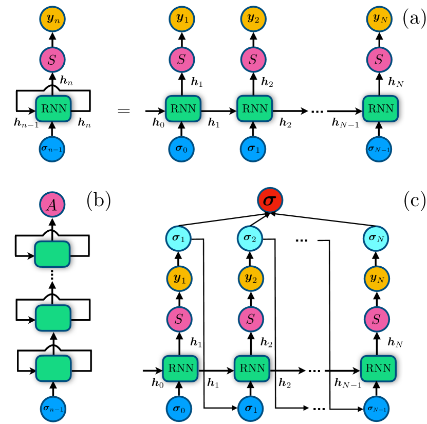
By construction, the model allows for an efficient estimation of the normalized probability of a given configuration . This construction is unlike energy-based models, which require intractable calculations of the partition function, or likelihood-free models such as Generative Adversarial Networks (GANs) that do not allow for an explicit estimation of probabilities Goodfellow (2016); Goodfellow et al. (2016). The sequential process of computing the probability vectors is schematically depicted in Fig. 1(a). Deep architectures can be obtained by stacking several RNN cells as shown in Fig. 1(b) for a general activation function (not necessarily Softmax). As illustrated in Fig. 1(c), RNNs have the autoregressive property, meaning that the conditional probability depends only on configurations . We also note that the computational cost of sampling a configuration is linear in the length of the configuration. Another important property of the normalized RNN probability distribution is that it can be used to produce successive samples and that are independent. Taking advantage of this property, the sampling procedure can be parallelized.
In practice, training vanilla RNNs can be challenging, since capturing long-distance correlations between the variables tends to make the gradients either explode or vanish Bengio et al. (1994); Kolen and Kremer (2001); Pascanu et al. (2013); Chung et al. (2014). Similar to MPS Fannes et al. (1992), long-distance correlations in RNNs are suppressed exponentially Shen (2019) and extensions of the vanilla RNN have been proposed Hochreiter and Schmidhuber (1997); Cho et al. (2014b) in order to improve on this limitation. Two successful examples are the long short-term memory (LSTM) unit Hochreiter and Schmidhuber (1997), and the gated recurrent unit (GRU) Cho et al. (2014b). Unless stated otherwise, in this paper we use the GRU Cho et al. (2014b) as the elementary cell in our (one-dimensional) RNNs to study models in one and two spatial dimensions. The details of the implementation can be found in App. A.
Furthermore, we explore the use of two-dimensional (2D) vanilla RNNs Graves (2012), where information about the spatial location of neighboring spins is exploited by the RNN ansatz. The basic idea of 2D RNNs is to replace the single recurrent connection in a standard RNN, as shown in Eq. (2), with two recurrent connections that are passed to the neighboring sites. Thus, at each point in the lattice the hidden layer of the network receives both spin configuration inputs and the hidden vectors from the neighboring sites, in a way that respects the autoregressive property. We provide the details of the implementation in Sec. III.3 and App. B.
II.2 RNN wave functions
The previous section focused exclusively on the efficient parametrization of classical probability distributions . In contrast, quantum mechanical wave functions are in general a set of complex valued amplitudes , rather than conventional probabilities. Before discussing how to modify the RNN ansatz to represent complex wave functions, we note that an important class of stoquastic many-body Hamiltonians has ground states with real and positive amplitudes in the standard product spin basis Bravyi et al. (2008). Thus, these ground states have representations in terms of probability distributions,
| (6) |
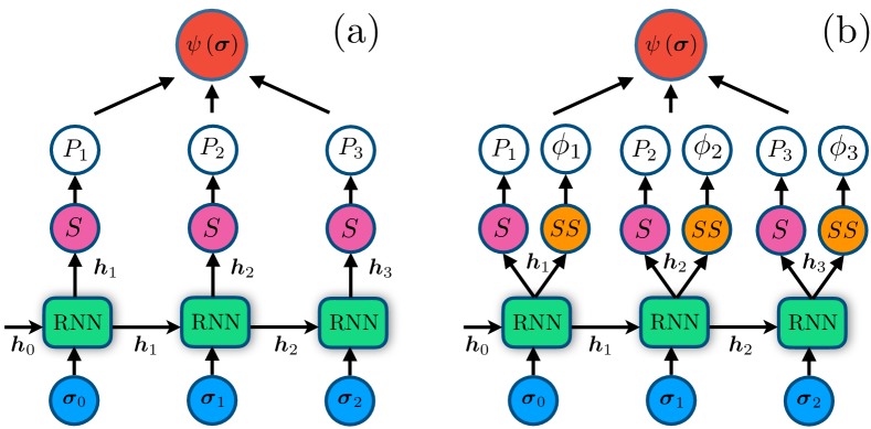
This property has been exploited extensively in wave function representations using generative models such as restricted Boltzmann machines Melko et al. (2019). For such wave functions, it is also natural to try to approximate with a conventional RNN, as illustrated in Fig. 2(a). For later reference we call this architecture a positive recurrent neural network wave function (pRNN wave function).
The generalization to the complex case starts by splitting the wave function into an amplitude and phase Torlai et al. (2018) as
| (7) |
As illustrated in Fig. 2(b), we use one RNN cell and a Softmax layer to model the probability, together with a Softsign layer (as defined below) to model the phase. In this parametrization, the first layer uses the Softmax activation function to get conditional probabilities as
| (8) |
where
| (9) |
in a similar fashion to Eq. (3). The Softsign layer is used to compute the phases as
| (10) |
where
| (11) |
The Softsign function is defined as
Finally, the probability is obtained from the individual contributions as
| (12) |
and, similarly, the phase is computed as
| (13) |
Note that sampling from the square of the amplitudes is unaffected by the Softsign layer and is carried out, as described above, using only the Softmax layer as in Fig. 1(c). For later reference, we call this architecture a complex recurrent neural network wave function (cRNN wave function), and hereafter, the term RNN wave function will refer to both pRNN wave functions and cRNN wave functions. Details about the dimensions of the variational parameters of RNN wave functions can be found in App. A.
III Ground States with RNN wave functions
We focus our attention on the ground state properties of prototypical Hamiltonians in condensed matter physics including the one- and two-dimensional (1D and 2D) transverse field Ising model (TFIM), as well as the 1D - model, both with open boundary conditions. Their Hamiltonians are given by
| (14) |
where are Pauli matrices acting on site , and
| (15) |
where is a spin-1/2 operator. Here, and denote nearest- and next-nearest-neighbor pairs, respectively. Energies for the - model are measured in units of in the results that follow.
To train our models we use the variational principle, where for a given problem Hamiltonian , the optimization strategy involves minimizing the expectation value with respect to the variational parameters . Here, is the exact ground state energy of . The variational parameters are updated using variants of the gradient descent algorithm with the objective of minimizing . We provide a detailed description of the VMC scheme and the optimization strategy with which we optimize our RNN wave functions in App. C.
Since the TFIM in Eq. (14) is stoquastic, the ground state is positive Bravyi et al. (2008) and hence we use the pRNN wave function ansatz. The - model with positive couplings, on the other hand, has a ground state endowed with a sign structure in the computational -basis, and thus we use a cRNN wave function ansatz.
In the following sections, we use 1D RNN wave functions to approximate the ground state problem of the 1D TFIM and the 1D - model, whereas we use both 1D and 2D pRNN wave functions in the case of the 2D TFIM.
III.1 1D transverse field Ising model
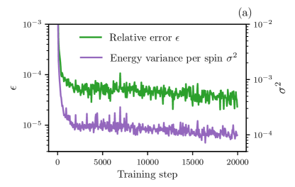
To demonstrate the power of our proposed method, we use it to target the ground state of a TFIM in one dimension with spins at the critical point using a pRNN wave function that has a single-layer RNN with memory units. In Fig. 3(a), we show the evolution of the relative error
| (16) |
and the energy variance per spin
| (17) |
as a function of the training step. is the ground state energy as obtained from a density matrix renormalization group (DMRG) calculation White (1992); Roberts et al. (2019), and can be considered exact in one dimension. We obtain very accurate results with a modest number of parameters (, see App. A). For comparison, the number of parameters of a restricted Boltzmann machine (RBM) Carleo and Troyer (2017) with one layer scales as with the number of hidden units and the number of physical spins. This scaling implies that the pRNN wave function here has the same number of variational parameters as an RBM with only eight hidden units.
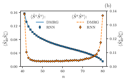
While energies and variances give a quantitative indication of the quality of a variational wave function, correlation functions provide a more comprehensive characterization. Indeed, correlation functions are at the heart of condensed matter theory since many experimental probes in condensed matter physics directly relate to measurements of correlation functions. Examples include inelastic scattering, which probes density-density correlation functions, and the Green’s function, out of which important thermodynamic properties of a quantum system can be computed Abrikosov et al. (1975). In Fig. 3(b) we compare the RNN results for the two-point correlation functions and with DMRG. Here, we see consistency between the RNN and the DMRG results.
Extracting entanglement entropy from many-body quantum systems is a central theme in condensed matter physics, with entanglement entropy providing an additional window into the structure of complex quantum states of matter beyond what is seen from correlation functions. Of particular interest is the family of Rényi entropies of order of a reduced density matrix ,
| (18) |
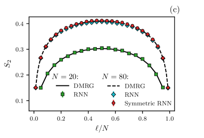
encodes important non-local properties of quantum many-body systems such as topological entanglement, and contains information about universal properties of quantum phases such as the central charge Flammia et al. (2009); Ryu and Takayanagi (2006). Due to their non-local character, extracting Rényi entropies from many-body quantum systems is notoriously difficult. Here, we use the so-called replica trick Hastings et al. (2010) to calculate the Rényi entropy for RNN wave functions. The details of the implementation can be found in App. E. In Fig. 3(c), we show results for the Rényi entropy for two different system sizes of 1D TFIM. here is the reduced density matrix on the first sites of the spin chain, obtained by tracing out all sites such that
| (19) |
Indeed for both system sizes, Fig. 3(c) shows excellent agreement between the pRNN wave function estimation and the DMRG result. To improve the overall quality of the quantum state, we have enforced the parity symmetry on our pRNN wave function (see App. D.1), denoted by “Symmetric RNN” in Fig. 3(c). We observe that the symmetric pRNN wave function leads to a more accurate estimate of for sites.
III.2 1D model
Moving beyond stoquastic Hamiltonians, we now investigate the performance of RNN wave functions for a Hamiltonian the ground state of which has a sign structure in the computational basis, specifically the - model in one dimension.
We use a variationally optimized deep cRNN wave function with three GRU layers, each with 100 memory units, to approximate the ground state of the - model. The phase diagram of this model has been studied with DMRG White and Affleck (1996), where it was found that the model exhibits a quantum phase transition at Eggert (1996); Becca et al. (2009) from a critical Luttinger liquid phase for to a spontaneously dimerized gapped valence bond state phase for .
We impose spin symmetry in the cRNN wave function (see App. D.2), and target the ground state at four different points . Note that at , the Hamiltonian in Eq. (15) can be made stoquastic by a local unitary transformation that rotates every other spin by around the -axis. The ground state can in this case be decomposed as Marshall (1955)
| (20) |
where is given by with Marshall (1955) and is the positive amplitude of the wave function. The set comprises the sites belonging to the sublattice of all even (or all odd) sites in the lattice. The prefactor is known as the Marshall sign of the wave function Marshall (1955). For , this decomposition is no longer exact, and acquires a non-trivial sign structure. For finite the decomposition in Eq. (20) can still be applied with the hope that the sign structure of remains close to the Marshall sign Choo et al. (2019a).
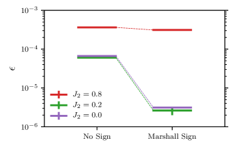
In Fig. 4, we compare ground state energies of the cRNN wave function trained on the 1D - model with spins with and without applying a Marshall sign. For small values of , we find a considerable improvement of the energies when applying the Marshall sign on top of the cRNN wave function. This observation highlights the importance of considering a prior “sign ansatz” to achieve better results. In the absence of a prior sign, the cRNN wave function can still achieve accurate estimations of the ground state energies, showing that cRNN wave functions can recover some of the unknown sign structure of the ground state. For , however, the improvement is less pronounced, which is expected due to the emergence of a second sign structure in the limit (when the system decouples into two independent unfrustrated Heisenberg chains) Torlai et al. (2019); Thibaut et al. (2019), that is widely different from the Marshall sign in Eq. (20). We omit from Fig. 4 our results at the point . In this case, the 1D - model reduces to the Majumdar-Ghosh model, where the ground state is a product-state of spin singlets, and we find agreement with the exact ground state energy within error bars when we apply an initial Marshall sign structure. We provide a summary of the cRNN wave function’s obtained values in App. F.
III.3 2D transverse field Ising model
Understanding strongly correlated quantum many-body systems in spatial dimensions is one of the central problems in condensed matter physics. During the last decade, numerical approaches such as tensor networks Verstraete and Cirac (2004); Yan et al. (2011); Evenbly and Vidal (2015), quantum Monte Carlo Sandvik (2010); Becca and Sorella (2017), and neural networks Carleo and Troyer (2017) have moved to the forefront of research in this area. Despite tremendous progress, however, solving correlated quantum many-body systems even in two dimensions remains a challenging problem. We now turn our attention to the application of our RNN wave function approach to the 2D quantum Ising model shown in Eq. (14) on a square lattice, a paradigmatic example of a strongly correlated quantum many-body system. This model has a quantum phase transition at a critical magnetic field that separates a magnetically ordered phase from a random paramagnet Blöte and Deng (2002).
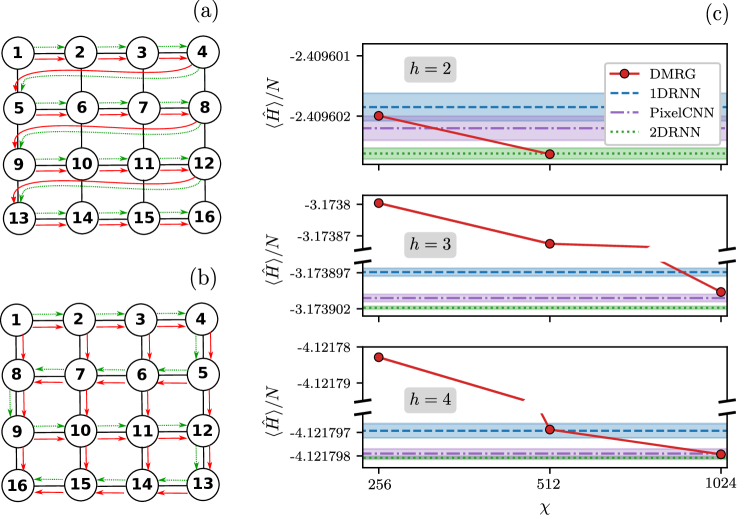
The simplest strategy for extending our approach to 2D geometries is to simply treat them as folded 1D chains, similar to the “snaking” approach used in 2D DMRG calculations (see Fig. 5(a)). While this approach works quite well, it has the fundamental drawback that neighboring sites on the lattice can become separated in the 1D geometry. As a consequence, local correlations in the 2D lattice are mapped into non-local correlations in the 1D geometry, which can increase the complexity of the problem considerably. For example, 2D DMRG calculations are typically restricted to 2D lattices with small width . This problem has led to the development of more powerful tensor network algorithms for 2D quantum systems such as projected entangled pair states (PEPS) Verstraete and Cirac (2004).
An advantage of RNN wave functions is their flexibility in how hidden vectors are passed between units. To obtain an RNN wave function more suited to a 2D geometry, we modify the simple 1D approach outlined above by allowing hidden vectors to also be passed vertically, instead of only horizontally, as described in App. B. This modification is illustrated by the red arrows in Fig. 5(b). We refer to this geometry in the following discussions as a 2D RNN. We optimize the 2D pRNN wave function with a single-layer 2D vanilla RNN cell that has 100 memory units (i.e. with variational parameters) to approximate the ground state of the 2D quantum Ising model at . The training complexity of the 2D pRNN wave function is only quadratic in the number of memory units (see App. B), which is very inexpensive compared to, e.g., the expensive variational optimization of PEPS, which scales as (where is the PEPS bond dimension and is the bond dimension of the intermediate MPS) Vanderstraeten et al. (2016).
For comparison, we also optimize a deep 1D pRNN wave function architecture with three layers of stacked GRU cells, each with 100 memory units (i.e., with 152000 variational parameters) for the same values of the magnetic field . In Fig. 5(c) we compare the obtained ground state energies with results from 2D DMRG calculations (run on the same 1D geometry as for the 1D pRNN wave function) and the PixelCNN architecture van den Oord et al. (2016a) (with 800000 variational parameters and results are taken from Ref. [Sharir et al., 2020]). For the magnetic fields shown above and for large bond dimensions, we obtain excellent agreement between all four methods. This agreement is particularly remarkable given that the 2D pRNN wave function uses only about 0.03% of the variational parameters of the DMRG calculation with bond dimension , about 2.6% of the variational parameters of the PixelCNN wave function used in Ref. [Sharir et al., 2020], and about 14% of the parameters used in the 1D pRNN architecture. A summary of our results in tabular form can be found in App. F.
III.4 Scaling of resources
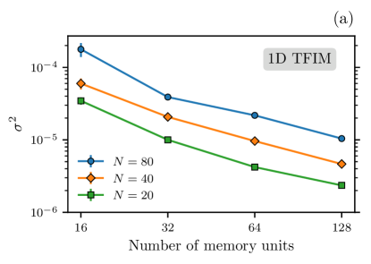
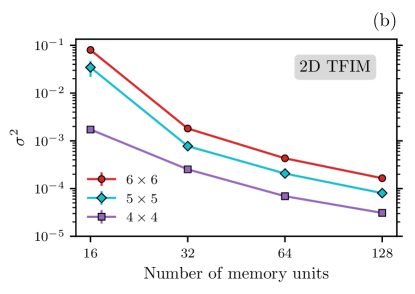
The optimization results of our RNN wave function approach depend on several hyperparameters, including the number of memory units, the number of recurrent layers in deep architectures, and the number of samples used to obtain the gradient during an optimization step (see App. C). Here, we investigate how the optimized energy and the energy variance per spin (see Eq. (17)) depend on these parameters. This energy variance per spin is an indicator of the quality of the optimized wave function, with exact eigenstates corresponding to . When targeting eigenstates, deviations from this value can be used to assess the quality of a variational wave function Gros (1990); Assaraf and Caffarel (2003); Becca and Sorella (2017), as previously done in the case of matrix product state based techniques Hubig et al. (2018); Bañuls et al. (2019). For variational approaches such as DMRG, one typically expects a non-zero value of that decreases when one increases the number of parameters (i.e., the expressivity) of the variational wave function. Since the number of variational parameters is directly related to the number of memory units of the pRNN wave function (see App. A), we study here the scaling of with the number of memory units.
In Fig. 6, we present the dependence of on the number of memory units for the 1D and 2D critical TFIMs. Fig. 6(a) shows results for for a 1D critical TFIM on three system sizes and , and Fig. 6(b) shows results for the 2D TFIM on and square lattices. In all cases, we used a single-layer 1D pRNN wave function and samples during optimization to compute estimates of the gradients. For each we observe a systematic decrease of (i.e., an increase in quality of the wave function) as we increase the number of memory units.
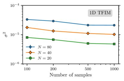
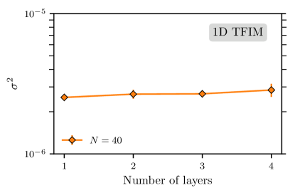
In App. G, we study the dependence of on both the number of samples and the number of layers in the pRNN wave function for a critical 1D TFIM. We observe only a weak dependence on both parameters. The weak dependence on the number of samples suggests that optimizing the RNN wave functions with noisy gradients does not significantly impact the results of the optimization procedure, and yields accurate estimations of the ground state and its energy. From the weak dependence on the number of layers we conclude that shallow RNNs with a sufficient number of memory units have enough expressivity and that deep architectures do not seem to be beneficial from an accuracy point of view. However, deeper networks could have potential ramifications regarding memory usage and training speed when it comes to training a large number of variational parameters, as shallow RNNs with a large number of memory units are equivalent in terms of number of parameters to deep RNNs with a smaller number of memory units. We also note that adding residual connections between layers Hermans and Schrauwen (2013) and dilated connections between RNN cells Chang et al. (2017) to deep RNNs, which we leave for future investigations, might change our previous conclusions and make deep RNNs more beneficial compared to shallow RNNs.
IV Conclusions and outlook
We have introduced recurrent neural network wave functions, a novel variational ansatz for quantum many-body systems, which we use to approximate ground state energies, correlation functions, and entanglement of many-body Hamiltonians of interest to condensed matter physics. We find that RNN wave functions are competitive with state-of-the-art methods such as DMRG and PixelCNN wave functions Sharir et al. (2020), performing particularly well on the task of finding the ground state of the transverse-field Ising model in two dimensions. By increasing the number of memory of units in the RNN, the error in our results can be systematically reduced. We have shown furthermore that we can accurately model ground states endowed with a sign structure using a complex recurrent neural network (cRNN) wave function ansatz. Here, accuracy can be improved by introducing an ansatz sign structure and by enforcing symmetries such as symmetry. The autoregressive nature of RNN wave functions makes it possible to directly generate independent samples, in contrast to methods based on Markov chain sampling, which are often plagued by long autocorrelation times that affect the optimization and the accurate estimation of correlation functions in a variational ansatz. Thanks to weight sharing among lattice sites, RNN wave functions provide very compact yet expressive representations of quantum states, while retaining the ability to easily train with millions of variational parameters, as opposed to, e.g., restricted Boltzmann machines Carleo and Troyer (2017). We expect that future work incorporating additional numerical techniques such as attention Bahdanau et al. (2014); Vaswani et al. (2017) and higher order optimization Becca and Sorella (2017); Martens et al. (2018) will make RNN wave functions a highly competitive tool for simulating quantum many-body systems, with applications to material science, quantum chemistry Choo et al. (2019b), quantum computation Carrasquilla et al. (2019b), and beyond.
Note added. A complementary paper on recurrent neural network wave functions Roth (2020) appeared after the publication of this manuscript.
Open-Source Code
Our code is made publicly available at “http://github.com/mhibatallah/RNNwavefunctions”. The hyperparameters we use are given in App. H.
Acknowledgments
We acknowledge Di Luo for his generous comments which were extremely helpful. We also thank Estelle Inack, Dan Sehayek, Amine Natik, Matthew Beach, Bohdan Kulchytskyy, Florian Hopfmueller, Roeland Wiersema, Giuseppe Carleo and Noam Wies for useful discussions and insights. M.H. acknowledges support of the Ecole Normale Superieure de Lyon. M.G. acknowledges support by the Simons Foundation (Many Electron Collaboration). R.G.M. acknowledges support from the Natural Sciences and Engineering Research Council of Canada (NSERC), a Canada Research Chair, the Shared Hierarchical Academic Research Computing Network (SHARCNET) and Compute Canada. J.C. acknowledges support from NSERC, SHARCNET, Compute Canada, and the Canadian institute for advanced research (CIFAR) AI chair program. Computer simulations were also made possible thanks to the Vector Institute computing cluster and Google Colaboratory. This research was supported in part by the National Science Foundation under Grant No. NSF PHY-1748958. It was also supported in part by the Perimeter Institute for Theoretical Physics. Research at Perimeter Institute is supported in part by the Government of Canada through Innovation, Science and Economic Development Canada (ISED) and by the Province of Ontario through the Ministry of Economic Development, Job Creation and Trade.
Appendix A Gated Recurrent Neural Networks
We use the GRU model introduced in Ref. [Cho et al., 2014b], which processes the spin configurations as
| (21) | ||||
where sig and tanh represent the sigmoid and hyperbolic tangent activation functions, respectively. Thus, the hidden vector is updated through an interpolation between the previous hidden state and a candidate hidden state . The update gate decides to what extent the contents of the hidden state are modified, and depends on how relevant the input is to the prediction (Softmax layer). The symbol denotes the pointwise (Hadamard) product. The reset gate modeled by the vector is such that if the -th component is close to zero, it cancels out the -th component of the hidden vector state , effectively making the GRU “forget” part of the sequence that has already been encoded in the state vector .
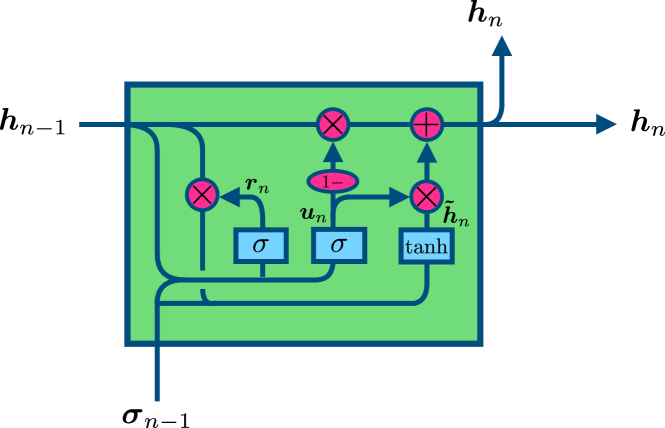
The weights matrices and the bias vectors parametrize the GRU and are optimized using energy minimization as described in App. C. The GRU transformations in Eq. (21) are depicted graphically in Fig. 7.
To take advantage of the GPU speed up, we use instead the cuDNN variant of GRUs implemented in Tensorflow Abadi et al. (2015), with
| (22) | ||||
which differs slightly from the above implementation of traditional GRU cells Appleyard et al. (2016).
Provided that the dimensions of the hidden state and input are and (respectively), then the dimensions of the variational parameters of a GRU as in Eq. (22) are
-
•
,
-
•
,
-
•
,
-
•
,
-
•
.
The new hidden state is fed into a Softmax layer to infer conditional probabilities, such that
and also into a Softsign layer to infer the phases as
We require the outputs to have dimension , so that each element of represents the conditional probability of sampling a value for the next spin , and that each element of corresponds to the phase of the chosen spin . Thus, the dimension of the parameters introduced in the Softmax/Softsign layer are
-
•
,
-
•
.
The same reasoning can be also applied to determine the dimensions of the variational parameters of 2D vanilla RNNs presented in App. B.
Appendix B Two-dimensional Recurrent Neural Network wave functions
Standard RNN architectures are inherently one dimensional. However, most interesting quantum many-body systems live in higher dimensions. By taking inspiration from Refs. [Graves, 2012] and [van den Oord et al., 2016b], we generalize one dimensional RNNs to multidimensional RNN wave functions. In particular, we generalize to 2D vanilla RNNs that are more suitable to simulating two-dimensional square lattices than one-dimensional RNNs, which map two-dimensional lattice configurations to one-dimensional configurations and do not necessarily encode spatial information about neighboring sites in a plausible manner.
The main idea behind the implementation of 2D RNNs Graves (2012) is to replace the single hidden state that is passed from one site to another by two hidden states, with each one corresponding to the state of a neighboring site (vertical and horizontal) and hence respecting the 2D geometry of the problem. To do so, we change the one-dimensional recursion relation in Eq. (2) to the two-dimensional recursion relation
| (23) |
where is the hidden state at site , are weight matrices and is a bias. Here is a non-linear activation function chosen to be equal to the exponential linear unit (ELU) defined as
The cost of computing a new hidden state is quadratic in the size of the hidden state (number of memory units ), and the cost of computing the gradients with respect to the variational parameters of the 2D RNN remains unchanged. This property allows us to train 2D RNNs with a relatively large .
To initialize the 2D RNN, we choose and to be null vectors. Once is computed, we apply the same scheme as in Sec. II.2 to sample a spin . The scheme for computing positive or complex amplitudes from Sec. II.2 remains the same.
We note that generalization to higher dimensions, to other lattices, as well as to other types of RNN architectures can be done by taking inspiration from this scheme. For instance, using LSTMs Hochreiter and Schmidhuber (1997), GRUs Cho et al. (2014b) or Transformers Vaswani et al. (2017) instead of vanilla RNNs in two dimensions is expected to make a significant improvement. We also expect that using multiplicative interactions Wu et al. (2016) might increase the expressiveness of 2D RNNs as compared to the additive interactions in Eq. (23).
Appendix C Variational Monte Carlo and Variance Reduction
The main goal of variational Monte Carlo (VMC) is to iteratively optimize an ansatz wave function to approximate, e.g., ground states of local Hamiltonians. VMC starts from a suitable trial wave function that incorporates the variational degrees of freedom of the approach. could be, for example, an MPS wave function Sandvik and Vidal (2007) in which case the free parameters are the MPS matrices. Crucially, the ansatz has to allow for efficient sampling from the square of the amplitudes of . In this paper, we choose RNN wave functions, described in Sec. II.2, to parametrize the trial wave function for a VMC optimization of ground states.
The aim of the VMC optimization is to minimize the expectation value of the energy
| (24) |
when given a family of states . This minimization is carried out using the gradient descent method or any of its variants. Since the RNN wave function is normalized such that , the expectation value in Eq. (24) can be written as
| (25) |
which represents a sample average of the local energy . The latter can be calculated efficiently for local Hamiltonians. Denoting to be the real variational parameters of , the gradients can be similarly written as
| (26) |
An optimization step consists of drawing samples from autoregressively using the RNN wave function, and then computing from Eq. (26) as
| (27) |
using automatic differentiation Zhang et al. (2019) and updating the parameters (if using gradient descent) according to
| (28) |
with a small learning rate . Instead of this simple gradient descent rule, we use the Adam optimizer Kingma and Ba (2014) to implement the gradient updates. We found that the latter gives better results compared to the simple gradient descent optimization shown in Eq. (28) and without having to carefully tune the learning rate .
We note that the stochastic evaluation of the gradients in Eq. (27) tends to carry noise that increases their variances Assaraf and Caffarel (1999); Clark (2010). Such high variances tend to slow down the convergence to the ground state energy. We propose to cure this limitation by introducing a new term in Eq. (27) that helps reduce the variance of the gradients by approximating
| (29) |
and we show below that this approximation does not introduce a bias. This new term is useful for reducing the uncertainty in the gradient estimation, as in the limit where near convergence, the variance of the gradients goes to zero as opposed to the nonzero variance of the gradients in Eq. (27). As a consequence, a stable convergence to the ground state is achieved as confirmed by our experiments. This idea is similar in spirit to control variate methods in Monte Carlo Assaraf and Caffarel (1999) and to baseline methods in reinforcement learning Mohamed et al. (2019).
To show that the term we add in Eq. (29) does not bias the true gradients in Eq. (26), it suffices to prove that
| (30) |
where denotes the statistical average over the probability distribution . To prove this expression, we write , which implies that
and hence
| (31) |
To show that Sutton et al. (2000); Mohamed et al. (2019), we write
where the fact that the RNN wave function is normalized justifies the transition from the third line to the fourth line.
From here, it suffices to show that . Since the Hamiltonian is Hermitian, the expectation value is real and hence . We therefore arrive at Eq. (30).
Appendix D Implementing Symmetries
D.1 Imposing discrete symmetries
Inspired by Refs. [Wu et al., 2019] and [Sharir et al., 2020], we propose to implement discrete symmetries in a similar fashion for RNN wave functions without spoiling their autoregressive nature.
Assuming that a Hamiltonian has a symmetry under discrete transformations , its ground state
is an eigenvector of the symmetry transformation . The ground state transforms as where is an eigenvalue with module 1, that is independent of the choice of . This expression implies that the transformation changes the ground state with only a global phase term that does not affect the probability distribution, and changes the sign structure with a global phase term. It is thus desirable that the RNN wave function also has this symmetry.
To enforce a discrete symmetry on an RNN wave function , we propose the following scheme:
-
•
Generate a sample autoregressively from the RNN wave function.
-
•
Sample with a probability a transformation from the symmetry transformation group that leaves the Hamiltonian invariant, and apply the transformation to .
-
•
Assign to the spin configuration the amplitude , such that
where is a probability generated by the Softmax layer and is a phase generated by the Softsign layer, as explained in Sec. II.2.
If the ground state is positive Bravyi et al. (2008), we use the same algorithm but only symmetrize the probability , without having to worry about symmetrizing the phase .
For concreteness, we illustrate the algorithm above with “Symmetric RNNs” that have a built-in parity symmetry. We use this architecture in Sec. III.1 to get a more accurate estimate of the ground state of the 1D TFIM that also obeys a parity symmetry. Indeed, symmetric RNNs show an improvement over ordinary pRNN wave functions on the task of estimating the second Rényi entropy (see App. E). Symmetric RNNs can be implemented using the following procedure:
-
•
Sample each configuration .
-
•
Choose to apply or to not apply the parity transformation on with a probability .
-
•
Assign to the probability:
We also emphasize the possibility of carefully designing RNN wave functions to impose discrete symmetries, without using the symmetrization scheme above and which we leave for future investigations.
D.2 Imposing zero magnetization
Since the ground state of the - model has zero magnetization, i.e., a symmetry Marshall (1955); Lieb and Mattis (1962), it is helpful to enforce this constraint on our RNN wave functions to get accurate estimations of the ground state energy. To do so, we propose an efficient way to generate samples with zero magnetization while maintaining the autoregressive property of the RNN wave function. The procedure effectively applies a projector to the original state, which restricts the RNN wave function to the subspace of configurations with zero magnetization. This procedure avoids generating a large number of samples and discarding the ones that have non-zero magnetization.
The condition of zero magnetization implies that the number of up spins should be equal to the number of down spins. To satisfy this constraint, we utilize the following algorithm:
-
•
Sample autoregressively the first half of the spin configuration
-
•
At each step :
-
–
Generate the output of the RNN wave function: where and are both non-zero and their modules squared sum to .
-
–
Define the following amplitudes:
where
and
In words, is the number of up/down spins generated before step .
-
–
Sample from , where:
which is normalized, i.e. .
-
–
Using this algorithm, it is clear that the RNN wave function generates a spin configuration that has the same number of up spins and down spins, and hence a zero magnetization. In fact, at each step , the function assigns a zero amplitude for the next spin to be spin up if or to be spin down if .
Interestingly enough, our scheme does not spoil the normalization of the RNN wave function as the new conditional probabilities are also normalized. We also note that this algorithm preserves the autoregressive property of the original RNN wave function and can also be parallelized. Moreover, this scheme can be easily extended to the generation of samples with a non-zero fixed magnetization, which is useful when considering the problem of finding states that live in a non-zero fixed magnetization sector.
Appendix E Rényi entropies
Given a quantum system with a spatial bipartition , one can write the RNN wave function as
where denotes the spin configuration that lives in the partition and stands for a concatenation of and .
The -Rényi entropy between region and is given by
| (32) |
where and is an integer Hastings et al. (2010). To estimate these entropies, we use the so-called replica trick Hastings et al. (2010), where we consider the action of the operator on the two copies of the RNN wave function, which swaps the spins in the region between the two copies (as demonstrated in Fig. 8) such that
| (33) |
The expectation value of in the double copy of the RNN wave function “” is given by Hastings et al. (2010); Torlai et al. (2018)
| (34) |
Hence, by calculating the expectation of the value of the Swap operator in the double copy of the RNN wave function, we can access the second Rényi entropy. Interestingly, the Rényi entropies have been shown to encode similar properties independently of Hastings et al. (2010); Flammia et al. (2009).
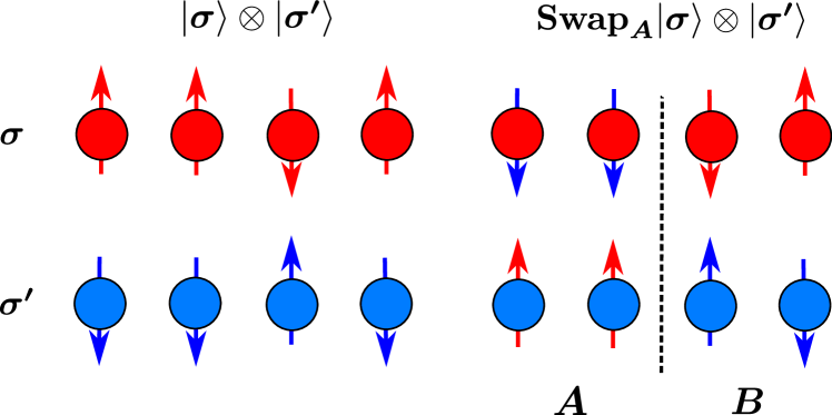
Although an exact evaluation of Eq. (34) is numerically intractable, we can use importance sampling to estimate it Hastings et al. (2010) as
| (35) |
Using this trick, for the system sizes studied in this paper we only have to generate two sets of exact samples and independently from without having to use the improved ratio trick Hastings et al. (2010). By defining
the statistical error on the estimation of the Rényi-2 entropy can be calculated as
For the estimation of the Rényi-2 entropy for the 1D TFIM in this paper, we use samples from a trained RNN wave function with one GRU layer and memory units.
During the completion of this paper, we became aware of another way to estimate entanglement entropies using autoregressive models with conditional sampling Wang and Davis (2020).
Appendix F Tables of Results
In Tab. 1, we state the variational energies of the cRNN wave function for the 1D - model and compare with results from DMRG. We examine two different methods of training. First, we do not impose an initial sign structure while, secondly, we introduce a background Marshall sign. The results suggest that using a Marshall sign improves the results significantly for and (with for all cases).
| No Sign | Marshall Sign | DMRG | |
| -0.4412480(2) | -0.4412760(1) | -0.4412773 | |
| -0.4073635(3) | -0.4073871(3) | -0.4073881 | |
| -0.3749958(6) | -0.3750006(6) | -0.3750000 | |
| -0.4205478(13) | -0.4205695(12) | -0.4207006 | |
In Tab. 2, we compare the variational energies per site of the 2D TFIM with a lattice size of for different values of the transverse magnetic field , for a 1D pRNN wave function, a 2D pRNN wave function, a PixelCNN wave function Sharir et al. (2020) and DMRG.
| 1DRNN | 2DRNN | PixelCNN | DMRG | |
| -2.4096018(2) | -2.40960262(9) | -2.4096022(2) | -2.40960263 | |
| -3.1738969(5) | -3.1739018(2) | -3.1739005(5) | -3.17389966 | |
| -4.1217969(3) | -4.12179808(6) | -4.1217979(2) | -4.12179793 | |
Appendix G Scaling of resources (continued)
Fig. 9 shows the dependence of on the number of samples used to estimate the gradients of the variational energy (see App. C). We investigate this effect for the case of the 1D TFIM, using 50 memory units in the pRNN wave function. Even though a large number of samples yields higher statistical accuracy of the gradient estimates used in our optimizations, we observe only a weak dependence of on the number of samples for all studied system sizes.
In Fig. 10 we present results for the dependence of on the depth of the pRNN wave function architecture for a critical TFIM with sites. We investigate architectures up to a depth of four layers. The number of memory units is adapted such that we have a similar number of variational parameters (31000) for each of the four architectures. We find that depends only weakly on the number of layers.
Appendix H Hyperparameters
In Tab. 3, we present the hyperparameters used to train the RNN wave functions in this paper. We anticipate that further improvements such as the use of stochastic reconfiguration Becca and Sorella (2017) or a computationally cheaper variant such as K-FAC Martens et al. (2018) for the optimization could potentially lead to more accurate estimations of the ground state energies as compared to the Adam optimizer Kingma and Ba (2014). Seeds are listed in the table for reproducibility purposes.
| Figures | Hyperparameter | Value |
| Fig. 3 | Architecture | One-layer 1D pRNN wave function with memory units |
| Number of samples | (), (), () | |
| Training iterations | ||
| Learning rate | | |
| Seed | ||
| Fig. 4 | Architecture | Three-layer 1D cRNN wave function with memory units |
| Number of samples | 500 | |
| Training iterations | ||
| Learning rate | with | |
| Seed | ||
| Fig. 5(c): 1DRNN | Architecture | Three-layer 1D pRNN wave function with memory units |
| Number of samples | ||
| Training iterations | ||
| Learning rate | with | |
| Seed | ||
| Fig. 5(c): 2DRNN | Architecture | One-layer 2D pRNN wave function with memory units |
| Number of samples | ||
| Training iterations | ||
| Learning rate | with | |
| Seed | ||
| Fig. 6(a) | Architecture | One-layer 1D pRNN wave function |
| Number of samples | ||
| Training iterations | ||
| Learning rate | ||
| Seeds | ||
| Fig. 6(b) | Architecture | One-layer 1D pRNN wave function |
| Number of samples | ||
| Training iterations | ||
| Learning rate | with | |
| Seeds | ||
| Fig. 9 | Architecture | One-layer 1D pRNN wave function with memory units |
| Training iterations | ||
| Learning rate | ||
| Seeds | ||
| Fig. 10 | Architecture | 1D pRNN wave function |
| Number of samples | ||
| Training iterations | ||
| Learning rate | ||
| Seeds |
References
- Krizhevsky et al. (2012) Alex Krizhevsky, Ilya Sutskever, and Geoffrey E. Hinton, “Imagenet classification with deep convolutional neural networks,” in Proceedings of the 25th International Conference on Neural Information Processing Systems - Volume 1, NIPS’12 (Curran Associates Inc., Red Hook, NY, USA, 2012) p. 1097–1105.
- LeCun et al. (2015) Yann LeCun, Yoshua Bengio, and Geoffrey Hinton, “Deep learning,” Nature 521, 436 (2015).
- He et al. (2016) Kaiming He, Xiangyu Zhang, Shaoqing Ren, and Jian Sun, “Deep Residual Learning for Image Recognition,” in 2016 IEEE Conference on Computer Vision and Pattern Recognition (CVPR) (2016) pp. 770–778.
- Young et al. (2017) Tom Young, Devamanyu Hazarika, Soujanya Poria, and Erik Cambria, “Recent trends in deep learning based natural language processing,” (2017), arXiv:1708.02709 [cs.CL] .
- Vamathevan et al. (2019) Jessica Vamathevan, Dominic Clark, Paul Czodrowski, Ian Dunham, Edgardo Ferran, George Lee, Bin Li, Anant Madabhushi, Parantu Shah, Michaela Spitzer, and Shanrong Zhao, “Applications of machine learning in drug discovery and development,” Nature Reviews Drug Discovery 18, 463–477 (2019).
- Badue et al. (2019) Claudine Badue, Rânik Guidolini, Raphael Vivacqua Carneiro, Pedro Azevedo, Vinicius Brito Cardoso, Avelino Forechi, Luan Jesus, Rodrigo Berriel, Thiago Paixão, Filipe Mutz, Lucas Veronese, Thiago Oliveira-Santos, and Alberto Ferreira De Souza, “Self-driving cars: A survey,” (2019), arXiv:1901.04407 [cs.RO] .
- Silver et al. (2017) David Silver, Julian Schrittwieser, Karen Simonyan, Ioannis Antonoglou, Aja Huang, Arthur Guez, Thomas Hubert, Lucas Baker, Matthew Lai, Adrian Bolton, Yutian Chen, Timothy Lillicrap, Fan Hui, Laurent Sifre, George van den Driessche, Thore Graepel, and Demis Hassabis, “Mastering the game of go without human knowledge,” Nature 550, 354–359 (2017).
- Carleo et al. (2019) Giuseppe Carleo, Ignacio Cirac, Kyle Cranmer, Laurent Daudet, Maria Schuld, Naftali Tishby, Leslie Vogt-Maranto, and Lenka Zdeborová, “Machine learning and the physical sciences,” Reviews of Modern Physics 91 (2019), 10.1103/revmodphys.91.045002.
- Carleo and Troyer (2017) Giuseppe Carleo and Matthias Troyer, “Solving the quantum many-body problem with artificial neural networks,” Science 355, 602–606 (2017).
- Hohenberg and Kohn (1964) P. Hohenberg and W. Kohn, “Inhomogeneous electron gas,” Phys. Rev. 136, B864–B871 (1964).
- Bardeen et al. (1957) J. Bardeen, L. N. Cooper, and J. R. Schrieffer, “Theory of superconductivity,” Phys. Rev. 108, 1175–1204 (1957).
- Laughlin (1983) R. B. Laughlin, “Anomalous quantum hall effect: An incompressible quantum fluid with fractionally charged excitations,” Phys. Rev. Lett. 50, 1395–1398 (1983).
- Becca and Sorella (2017) F. Becca and S. Sorella, Quantum Monte Carlo Approaches for Correlated Systems (Cambridge University Press, 2017).
- Orús (2019) Román Orús, “Tensor networks for complex quantum systems,” Nature Reviews Physics 1, 538–550 (2019).
- Peruzzo et al. (2014) Alberto Peruzzo, Jarrod McClean, Peter Shadbolt, Man-Hong Yung, Xiao-Qi Zhou, Peter J. Love, Alán Aspuru-Guzik, and Jeremy L. O’Brien, “A variational eigenvalue solver on a photonic quantum processor,” Nature Communications 5, 1–7 (2014).
- Androsiuk et al. (1993) J. Androsiuk, L. Kulak, and K. Sienicki, “Neural network solution of the Schrödinger equation for a two-dimensional harmonic oscillator,” Chemical Physics 173, 377–383 (1993).
- LAG (1997) “Artificial neural network methods in quantum mechanics,” Computer Physics Communications 104, 1 – 14 (1997).
- Sugawara (2001) M. Sugawara, “Numerical solution of the Schrödinger equation by neural network and genetic algorithm,” Computer Physics Communications 140, 366–380 (2001).
- Melko et al. (2019) Roger G. Melko, Giuseppe Carleo, Juan Carrasquilla, and J. Ignacio Cirac, “Restricted Boltzmann machines in quantum physics,” Nature Physics , 1 (2019).
- Hochreiter and Schmidhuber (1997) Sepp Hochreiter and Jürgen Schmidhuber, “Long short-term memory,” Neural Comput. 9, 1735–1780 (1997).
- Graves (2012) Alex Graves, “Supervised sequence labelling,” in Supervised sequence labelling with recurrent neural networks (Springer, 2012) pp. 5–13.
- Cho et al. (2014a) Kyunghyun Cho, Bart van Merrienboer, Caglar Gulcehre, Dzmitry Bahdanau, Fethi Bougares, Holger Schwenk, and Yoshua Bengio, “Learning phrase representations using rnn encoder-decoder for statistical machine translation,” (2014a), arXiv:1406.1078 [cs.CL] .
- Chung et al. (2014) Junyoung Chung, Caglar Gulcehre, KyungHyun Cho, and Yoshua Bengio, “Empirical evaluation of gated recurrent neural networks on sequence modeling,” (2014), arXiv:1412.3555 [cs.NE] .
- Lipton et al. (2015) Zachary C. Lipton, John Berkowitz, and Charles Elkan, “A critical review of recurrent neural networks for sequence learning,” (2015), arXiv:1506.00019 [cs.LG] .
- Vaswani et al. (2017) Ashish Vaswani, Noam Shazeer, Niki Parmar, Jakob Uszkoreit, Llion Jones, Aidan N. Gomez, Lukasz Kaiser, and Illia Polosukhin, “Attention is all you need,” (2017), arXiv:1706.03762 [cs.CL] .
- Devlin et al. (2018) Jacob Devlin, Ming-Wei Chang, Kenton Lee, and Kristina Toutanova, “Bert: Pre-training of deep bidirectional transformers for language understanding,” (2018), arXiv:1810.04805 [cs.CL] .
- Yang et al. (2019) Zhilin Yang, Zihang Dai, Yiming Yang, Jaime Carbonell, Ruslan Salakhutdinov, and Quoc V. Le, “Xlnet: Generalized autoregressive pretraining for language understanding,” (2019), arXiv:1906.08237 [cs.CL] .
- Carrasquilla et al. (2019a) Juan Carrasquilla, Giacomo Torlai, Roger G. Melko, and Leandro Aolita, “Reconstructing quantum states with generative models,” Nature Machine Intelligence 1, 155–161 (2019a).
- Levine et al. (2019) Yoav Levine, Or Sharir, Nadav Cohen, and Amnon Shashua, “Quantum entanglement in deep learning architectures,” Phys. Rev. Lett. 122, 065301 (2019).
- Bengio and Bengio (2000) S. Bengio and Y. Bengio, “Taking on the curse of dimensionality in joint distributions using neural networks,” IEEE Transactions on Neural Networks 11, 550–557 (2000).
- Uria et al. (2016) Benigno Uria, Marc-Alexandre Côté, Karol Gregor, Iain Murray, and Hugo Larochelle, “Neural autoregressive distribution estimation,” J. Mach. Learn. Res. 17, 7184–7220 (2016).
- Wu et al. (2019) Dian Wu, Lei Wang, and Pan Zhang, “Solving statistical mechanics using variational autoregressive networks,” Physical Review Letters 122 (2019), 10.1103/physrevlett.122.080602.
- Goodfellow et al. (2016) Ian Goodfellow, Yoshua Bengio, and Aaron Courville, Deep Learning (MIT Press, 2016) http://www.deeplearningbook.org.
- Goodfellow (2016) Ian Goodfellow, “Nips 2016 tutorial: Generative adversarial networks,” (2016), arXiv:1701.00160 [cs.LG] .
- Bengio et al. (1994) Y. Bengio, P. Simard, and P. Frasconi, “Learning long-term dependencies with gradient descent is difficult,” IEEE Transactions on Neural Networks 5, 157–166 (1994).
- Kolen and Kremer (2001) J. F. Kolen and S. C. Kremer, “Gradient flow in recurrent nets: The difficulty of learning longterm dependencies,” in A Field Guide to Dynamical Recurrent Networks (IEEE, 2001) pp. 237–243.
- Pascanu et al. (2013) Razvan Pascanu, Tomas Mikolov, and Yoshua Bengio, “On the difficulty of training recurrent neural networks,” in International conference on machine learning (2013) pp. 1310–1318.
- Fannes et al. (1992) M. Fannes, B. Nachtergaele, and R. F. Werner, “Finitely correlated states on quantum spin chains,” Communications in Mathematical Physics 144, 443–490 (1992).
- Shen (2019) Huitao Shen, “Mutual information scaling and expressive power of sequence models,” (2019), arXiv:1905.04271 [cs.LG] .
- Cho et al. (2014b) Kyunghyun Cho, Bart van Merriënboer, Dzmitry Bahdanau, and Yoshua Bengio, “On the properties of neural machine translation: Encoder–decoder approaches,” in Proceedings of SSST-8, Eighth Workshop on Syntax, Semantics and Structure in Statistical Translation (Association for Computational Linguistics, Doha, Qatar, 2014) pp. 103–111.
- Bravyi et al. (2008) Sergey Bravyi, David P. Divincenzo, Roberto Oliveira, and Barbara M. Terhal, “The complexity of stoquastic local hamiltonian problems,” Quantum Info. Comput. 8, 361–385 (2008).
- Torlai et al. (2018) Giacomo Torlai, Guglielmo Mazzola, Juan Carrasquilla, Matthias Troyer, Roger Melko, and Giuseppe Carleo, “Neural-network quantum state tomography,” Nature Physics 14, 447 (2018).
- White (1992) Steven R. White, “Density matrix formulation for quantum renormalization groups,” Phys. Rev. Lett. 69, 2863–2866 (1992).
- Roberts et al. (2019) Chase Roberts, Ashley Milsted, Martin Ganahl, Adam Zalcman, Bruce Fontaine, Yijian Zou, Jack Hidary, Guifre Vidal, and Stefan Leichenauer, “Tensornetwork: A library for physics and machine learning,” (2019), arXiv:1905.01330 [physics.comp-ph] .
- Abrikosov et al. (1975) A A Abrikosov, I Dzyaloshinskii, L P Gorkov, and Richard A Silverman, Methods of quantum field theory in statistical physics (Dover, New York, NY, 1975).
- Flammia et al. (2009) Steven T. Flammia, Alioscia Hamma, Taylor L. Hughes, and Xiao-Gang Wen, “Topological entanglement rényi entropy and reduced density matrix structure,” Phys. Rev. Lett. 103, 261601 (2009).
- Ryu and Takayanagi (2006) Shinsei Ryu and Tadashi Takayanagi, “Holographic derivation of entanglement entropy from the anti–de sitter space/conformal field theory correspondence,” Phys. Rev. Lett. 96, 181602 (2006).
- Hastings et al. (2010) Matthew B. Hastings, Iván González, Ann B. Kallin, and Roger G. Melko, “Measuring renyi entanglement entropy in quantum monte carlo simulations,” Physical Review Letters 104 (2010), 10.1103/physrevlett.104.157201.
- White and Affleck (1996) Steven R. White and Ian Affleck, “Dimerization and incommensurate spiral spin correlations in the zigzag spin chain: Analogies to the kondo lattice,” Phys. Rev. B 54, 9862–9869 (1996).
- Eggert (1996) Sebastian Eggert, “Numerical evidence for multiplicative logarithmic corrections from marginal operators,” Phys. Rev. B 54, R9612–R9615 (1996).
- Becca et al. (2009) Federico Becca, Luca Capriotti, Alberto Parola, and Sandro Sorella, “Variational wave functions for frustrated magnetic models,” (2009), arXiv:0905.4854 [cond-mat.str-el] .
- Marshall (1955) W Marshall, “Antiferromagnetism,” Proceedings of the Royal Society of London. Series A. Mathematical and Physical Sciences 232, 48–68 (1955).
- Choo et al. (2019a) Kenny Choo, Titus Neupert, and Giuseppe Carleo, “Two-dimensional frustrated j1-j2 model studied with neural network quantum states,” Physical Review B 100 (2019a), 10.1103/physrevb.100.125124.
- Torlai et al. (2019) Giacomo Torlai, Juan Carrasquilla, Matthew T. Fishman, Roger G. Melko, and Matthew P. A. Fisher, “wave function positivization via automatic differentiation,” (2019), arXiv:1906.04654 [quant-ph] .
- Thibaut et al. (2019) Jérôme Thibaut, Tommaso Roscilde, and Fabio Mezzacapo, “Long-range entangled-plaquette states for critical and frustrated quantum systems on a lattice,” Physical Review B 100 (2019), 10.1103/physrevb.100.155148.
- Sharir et al. (2020) Or Sharir, Yoav Levine, Noam Wies, Giuseppe Carleo, and Amnon Shashua, “Deep autoregressive models for the efficient variational simulation of many-body quantum systems,” Physical Review Letters 124 (2020), 10.1103/physrevlett.124.020503.
- Verstraete and Cirac (2004) F. Verstraete and J. I. Cirac, “Renormalization algorithms for quantum-many body systems in two and higher dimensions,” (2004), arXiv:cond-mat/0407066 [cond-mat.str-el] .
- Yan et al. (2011) Simeng Yan, David A. Huse, and Steven R. White, “Spin-liquid ground state of the s = 1/2 kagome heisenberg antiferromagnet,” Science 332, 1173–1176 (2011).
- Evenbly and Vidal (2015) G. Evenbly and G. Vidal, “Tensor network renormalization,” Phys. Rev. Lett. 115, 180405 (2015).
- Sandvik (2010) Anders W. Sandvik, “Computational Studies of Quantum Spin Systems,” AIP Conference Proceedings 1297, 135–338 (2010).
- Blöte and Deng (2002) Henk W. J. Blöte and Youjin Deng, “Cluster monte carlo simulation of the transverse ising model,” Phys. Rev. E 66, 066110 (2002).
- Vanderstraeten et al. (2016) Laurens Vanderstraeten, Jutho Haegeman, Philippe Corboz, and Frank Verstraete, “Gradient methods for variational optimization of projected entangled-pair states,” Physical Review B 94 (2016), 10.1103/physrevb.94.155123.
- van den Oord et al. (2016a) Aaron van den Oord, Nal Kalchbrenner, Lasse Espeholt, koray kavukcuoglu, Oriol Vinyals, and Alex Graves, “Conditional image generation with pixelcnn decoders,” in Advances in Neural Information Processing Systems 29, edited by D. D. Lee, M. Sugiyama, U. V. Luxburg, I. Guyon, and R. Garnett (Curran Associates, Inc., 2016) pp. 4790–4798.
- Gros (1990) Claudius Gros, “Criterion for a good variational wave function,” Phys. Rev. B 42, 6835–6838 (1990).
- Assaraf and Caffarel (2003) Roland Assaraf and Michel Caffarel, “Zero-variance zero-bias principle for observables in quantum monte carlo: Application to forces,” The Journal of Chemical Physics 119, 10536–10552 (2003).
- Hubig et al. (2018) C. Hubig, J. Haegeman, and U. Schollwöck, “Error estimates for extrapolations with matrix-product states,” Physical Review B 97 (2018), 10.1103/physrevb.97.045125.
- Bañuls et al. (2019) Mari Carmen Bañuls, David A. Huse, and J. Ignacio Cirac, “How much entanglement is needed to reduce the energy variance?” (2019), arXiv:1912.07639 [quant-ph] .
- Hermans and Schrauwen (2013) Michiel Hermans and Benjamin Schrauwen, “Training and analysing deep recurrent neural networks,” in Advances in Neural Information Processing Systems 26, edited by C. J. C. Burges, L. Bottou, M. Welling, Z. Ghahramani, and K. Q. Weinberger (Curran Associates, Inc., 2013) pp. 190–198.
- Chang et al. (2017) Shiyu Chang, Yang Zhang, Wei Han, Mo Yu, Xiaoxiao Guo, Wei Tan, Xiaodong Cui, Michael Witbrock, Mark Hasegawa-Johnson, and Thomas S. Huang, “Dilated recurrent neural networks,” (2017), arXiv:1710.02224 [cs.AI] .
- Bahdanau et al. (2014) Dzmitry Bahdanau, Kyunghyun Cho, and Yoshua Bengio, “Neural machine translation by jointly learning to align and translate,” (2014), arXiv:1409.0473 [cs.CL] .
- Martens et al. (2018) James Martens, Jimmy Ba, and Matt Johnson, “Kronecker-factored curvature approximations for recurrent neural networks,” in International Conference on Learning Representations (2018).
- Choo et al. (2019b) Kenny Choo, Antonio Mezzacapo, and Giuseppe Carleo, “Fermionic neural-network states for ab-initio electronic structure,” (2019b), arXiv:1909.12852 [physics.comp-ph] .
- Carrasquilla et al. (2019b) Juan Carrasquilla, Di Luo, Felipe Pérez, Ashley Milsted, Bryan K. Clark, Maksims Volkovs, and Leandro Aolita, “Probabilistic simulation of quantum circuits with the transformer,” (2019b), arXiv:1912.11052 [cond-mat.str-el] .
- Roth (2020) Christopher Roth, “Iterative retraining of quantum spin models using recurrent neural networks,” (2020), arXiv:2003.06228 [physics.comp-ph] .
- Abadi et al. (2015) Martín Abadi, Ashish Agarwal, Paul Barham, Eugene Brevdo, Zhifeng Chen, Craig Citro, Greg S. Corrado, Andy Davis, Jeffrey Dean, Matthieu Devin, Sanjay Ghemawat, Ian Goodfellow, Andrew Harp, Geoffrey Irving, Michael Isard, Yangqing Jia, Rafal Jozefowicz, Lukasz Kaiser, Manjunath Kudlur, Josh Levenberg, Dan Mané, Rajat Monga, Sherry Moore, Derek Murray, Chris Olah, Mike Schuster, Jonathon Shlens, Benoit Steiner, Ilya Sutskever, Kunal Talwar, Paul Tucker, Vincent Vanhoucke, Vijay Vasudevan, Fernanda Viégas, Oriol Vinyals, Pete Warden, Martin Wattenberg, Martin Wicke, Yuan Yu, and Xiaoqiang Zheng, “TensorFlow: Large-scale machine learning on heterogeneous systems,” (2015), software available from tensorflow.org.
- Appleyard et al. (2016) Jeremy Appleyard, Tomas Kocisky, and Phil Blunsom, “Optimizing performance of recurrent neural networks on gpus,” (2016), arXiv:1604.01946 [cs.LG] .
- van den Oord et al. (2016b) Aaron van den Oord, Nal Kalchbrenner, and Koray Kavukcuoglu, “Pixel recurrent neural networks,” (2016b), 1601.06759 [cs.CV] .
- Wu et al. (2016) Yuhuai Wu, Saizheng Zhang, Ying Zhang, Yoshua Bengio, and Ruslan R Salakhutdinov, “On multiplicative integration with recurrent neural networks,” in Advances in neural information processing systems (2016) pp. 2856–2864, 1606.06630 .
- Sandvik and Vidal (2007) A. W. Sandvik and G. Vidal, “Variational quantum monte carlo simulations with tensor-network states,” Phys. Rev. Lett. 99, 220602 (2007).
- Zhang et al. (2019) Shi-Xin Zhang, Zhou-Quan Wan, and Hong Yao, “Automatic differentiable monte carlo: Theory and application,” (2019), arXiv:1911.09117 [physics.comp-ph] .
- Kingma and Ba (2014) Diederik P. Kingma and Jimmy Ba, “Adam: A method for stochastic optimization,” (2014), arXiv:1412.6980 [cs.LG] .
- Assaraf and Caffarel (1999) Roland Assaraf and Michel Caffarel, “Zero-variance principle for monte carlo algorithms,” Physical Review Letters 83, 4682–4685 (1999).
- Clark (2010) Bryan Clark, “Variational monte carlo notes for boulder summer school 2010,” (2010).
- Mohamed et al. (2019) Shakir Mohamed, Mihaela Rosca, Michael Figurnov, and Andriy Mnih, “Monte carlo gradient estimation in machine learning,” (2019), arXiv:1906.10652 [stat.ML] .
- Sutton et al. (2000) Richard S Sutton, David A McAllester, Satinder P Singh, and Yishay Mansour, “Policy gradient methods for reinforcement learning with function approximation,” in Advances in neural information processing systems (2000) pp. 1057–1063.
- Lieb and Mattis (1962) Elliott Lieb and Daniel Mattis, “Ordering energy levels of interacting spin systems,” Journal of Mathematical Physics 3, 749–751 (1962).
- Wang and Davis (2020) Zhaoyou Wang and Emily J. Davis, “Calculating renyi entropies with neural autoregressive quantum states,” (2020), arXiv:2003.01358 [quant-ph] .