Parton Distribution Functions of the Charged Pion Within The xFitter Framework

Abstract

We present the first open-source analysis of parton distribution functions (PDFs) of charged pions using xFitter, an open-source QCD fit framework to facilitate PDF extraction and analyses. Our calculations are implemented at NLO using APPLgrids generated by MCFM. Using currently available Drell-Yan and photon production data, we find the valence distribution is well-constrained; however, the considered data are not sensitive enough to unambiguously determine sea and gluon distributions. Fractions of momentum carried by the valence, sea and gluon components are discussed, and we compare with the JAM and GRVPI1 results.

Introduction

The pion plays an important role in our understanding of strong interactions. At the same time, it is a mediator of nucleon-nucleon interactions, a pseudo-Goldstone boson of dynamical chiral symmetry breaking and the simplest $q\bar{q}$ state in the quark-parton model of hadrons. However, from the experimental point of view, the pion structure is currently poorly understood, especially compared to the proton. Parton distribution functions (PDFs) are a primary theoretical construct used to describe hadron structure as it is probed in hard processes. Much progress has been made in mapping out the parton distribution functions of the proton in the last decadesGao et al. (2018).

On the other hand, theoretically, the pion is a simpler system than the proton. Consequently, the pion structure has been investigated in several nonperturbative theoretical models. Nambu-Jona-Lasinio modelHatsuda and Kunihiro (1987); Klevansky (1992); Davidson and Ruiz Arriola (2002), Dyson-Schwinger equationsNguyen et al. (2011); Chang and Thomas (2015); Chen et al. (2016); Shi et al. (2018); Bednar et al. (2018); Ding et al. (2020a, b) (DSE), meson cloud modelSzczurek et al. (1996), and nonlocal chiral-quark modelNam (2012); Watanabe et al. (2016, 2018) make predictions about certain aspects of PDFs of the charged pion, or even allow calculating PDFs themselves. In the lattice QCD approach first moments of the valence pion PDF have been calculatedBest et al. (1997); Detmold et al. (2003); Abdel-Rehim et al. (2015), and direct computation of PDF has recently been achievedChen et al. (2018); de Teramond et al. (2018); Sufian et al. (2019, 2020).

Experimentally, the pion PDF is known mostly from QCD analyses of Drell-Yan (DY) and prompt photon production dataOwens (1984); Aurenche et al. (1989); Sutton et al. (1992); Wijesooriya et al. (2005). Within a dynamical approach, only the relatively well-known valence distribution is determined from DY data, with the sea and gluon content at a very low initial scale fixed by simplifying assumptionsGluck et al. (1992) or constraints of the constituent quark modelGluck et al. (1998, 1999). While all modern pion PDF extractions are performed at next-to-leading order (NLO), additional threshold-resummation corrections and their impact on the valence distribution at high $x$ have been studiedAicher et al. (2010). In addition to DY data, a recent work by the JAM collaborationBarry et al. (2018) included leading neutron (LN) electroproduction data obtained from the HERA collider (as suggested in Holtmann et al. (1994)). The latest pion PDF fit by Bourelly and SofferBourrely and Soffer (2019) uses a novel parameterisation at the initial scale $Q_{0}$.

In this analysis we approach the pion PDFs from a phenomenological context and introduce a number of unique features which provide a complementary perspective relative to other determinations. In particular, the combination of DY (E615 and NA10) and prompt photon (WA70) data provide constraints on both the quarks and gluons in our kinematic range. We also explore the theoretical uncertainties including variations of the strong coupling, as well as the factorization and renormalization scales; consequently, our PDF error bands reflect both the experimental and theoretical uncertainties. Our analysis uses MCFM generated APPLgrids which allow for efficient numerical computations; additionally, we implemented modifications to APPLgrid which allow both meson and hadron PDFs in the initial state. This work is implemented in the publicly available xFitter PDF fitting frameworkAlekhin et al. (2015); as such, it is the first open-source analysis of pion PDFs, and this will facilitate future studies of meson PDFs as new data become available.

The paper is organised as follows: In Section I we briefly discuss the considered data. The adopted PDF parameterisation and decomposition are described in Section II. Calculation of theoretical predictions is discussed in Section III. Section IV is devoted to the statistical treatment used in this work and estimation of the uncertainty of the obtained PDFs. Finally, the results of the analysis are presented and compared to results of other studies in Section V.

I Experimental data

This analysis is based on Drell-Yan data from NA10Betev et al. (1985) and E615Conway et al. (1989) experiments, and on photon production data from the WA70Bonesini et al. (1988) experiment. The NA10 and E615 experiments studied scattering of a $\pi^{-}$ beam off a tungsten target, with $E_{\pi}=194$ and $286\ \text{GeV}$ in the NA10 experiment and $E_{\pi}=252\ \text{GeV}$ in the E615 experiment. The WA70 experiment used $\pi^{\pm}$ beams and a proton target. For the Drell-Yan data, the $\Upsilon$-resonance range, which corresponds to bins with $\sqrt{\tau}\in[0.415,0.484]$, were excluded from the analysis. Here $\sqrt{\tau}=m_{\mu\mu}/\sqrt{s}$, $m_{\mu\mu}$ is the invariant mass of the muon pair, and $\sqrt{s}$ is the center-of-mass energy of pion-nucleon system.

Figure 1: Leading order Feynman diagrams for the considered processes: Drell-Yan dimuon production (left) and direct photon production (center and right).

Leading order Feynman diagrams for the considered processes are shown in Fig. 1. The Drell-Yan data constrain the valence distribution relatively well, but are not sensitive to sea and gluon distributions. The prompt photon production data complement the DY data by providing some sensitivity to the gluon distribution, but have smaller statistics and large uncertainties in comparison to the DY data. Additionally, the predictions for prompt photon production have significant theoretical uncertainty, as discussed in Section III.

II PDF Parameterisation

The $\pi^{-}$ PDF $xf(x,Q^{2})$ is parameterized at an initial scale $Q_{0}^{2}=1.9\ \text{GeV}^{2}$, just below the charm mass threshold $m_{c}^{2}=2.04\ \text{GeV}^{2}$. Neglecting electroweak corrections and quark masses, charge symmetry is assumed: $d=\bar{u}$, and SU(3)-symmetric sea: $u=\bar{d}=s=\bar{s}$. Under these assumptions, pion PDFs are reduced to three distributions: total valence $v$, total sea $S$, and gluon $g$:

$$v =d_{v}-u_{v}=(d-\bar{d})-(u-\bar{u})=2(d-u)=2d_{v},$$

$$S =2u+2\bar{d}+s+\bar{s}=6u,$$

$$g =g,$$

which we parameterise using a generic form:

$$xv(x) =A_{v}x^{B_{v}}(1-x)^{C_{v}}(1+D_{v}x^{\alpha}),$$

$$xS(x) =A_{S}x^{B_{S}}(1-x)^{C_{S}}/\mathcal{B}(B_{S}+1,C_{S}+1),$$ (1)

$$xg(x) =A_{g}(C_{g}+1)(1-x)^{C_{g}},$$

where $\mathcal{B}$ is the Euler beta function, which ensures that the $A_{S}$ parameter represents the total momentum fraction carried by the sea quarks. The $B$-parameters determine the low-$x$ behavior, and $C$-parameters determine the high-$x$ behavior. Quark-counting and momentum sum rules have the following form for $\pi^{-}$:

$$\int_{0}^{1}\hskip-5.69054ptv(x)\textrm{d}x =2, \int_{0}^{1}\hskip-5.69054ptx(v(x)+S(x)+g(x))\textrm{d}x =1.$$ (2)

The sum rules determine the values of parameters $A_{v}$ and $A_{g}$, respectively. The constant factors in the definitions of $v$, $S$, $g$ were chosen in such a way, that $\langle xv\rangle,\langle xS\rangle,\langle xg\rangle$ are momentum fractions of pion carried by the valence quarks, sea quarks, and gluons, respectively (here $\langle xf\rangle=\int_{0}^{1}xf(x)\textrm{d}x$).

The extension $D_{v}x^{\alpha}$ was introduced in $xv(x)$ to mitigate possible bias due to inflexibility of the chosen parameterisation. This extension was omitted in the initial fits ($D_{v}=0$). Afterwards, a parameterisation scan was performed by repeating the fit with free $D_{v}$ and different fixed values of parameter $\alpha$. The scan showed that only $\alpha=\frac{5}{2}$ has noticeably improved the quality of the fit (see Table 1 and Section V for discussion). The additional free parameter $D_{v}$ changes the shape of the valence distribution only slightly (Fig. 2). Similar attempts to add more parameters of the form $(1+D_{v}x^{\alpha}+E_{v}x^{\beta})$ did not result in significant improvement of $\chi^{2}$. The final presented results use a free $D_{v}$ and $\alpha=\frac{5}{2}$.

Table 1: Fitted parameter values and $\chi^{2}$. The first column corresponds to the fit with $D_{v}=0$. The second column shows results of the fit with free $D_{v}$ and $\alpha=\frac{5}{2}$. The uncertainties of parameter values do not include scale variations. The valence and gluon normalization parameters $A_{v}$ and $A_{g}$ were not fitted, but were determined based on sum rules (Eq.(2)) and values of the fitted parameters.

	$D_{v}$=0	free $D_{v}$
$\chi^{2}/N_{\text{DoF}}$	444/373=1.19	437/372=1.18
$A_{v}$	$2.60$	$1.72$
$\langle xv\rangle$	$0.56$	$0.54$
$B_{v}$	$0.75\pm 0.03$	$0.63\pm 0.06$
$C_{v}$	$0.95\pm 0.03$	$0.26\pm 0.13$
$D_{v}$	$0$	$-0.93\pm 0.06$
$A_{S}=\langle xS\rangle$	$0.21\pm 0.08$	$0.25\pm 0.09$
$B_{S}$	$0.5\pm 0.8$	$0.3\pm 0.7$
$C_{S}$	$8\pm 3.$	$6\pm 3.$
$A_{g}=\langle xg\rangle$	$0.23$	$0.20$
$C_{g}$	$3\pm 1.$	$3\pm 1.$

III Cross-section calculation

PDFs are evolved up from the starting scale $Q_{0}^{2}$ by solving the DGLAP equations numerically using QCDNUMBotje (2011). The evolution is performed using the variable flavor-number scheme with quark mass thresholds at $m_{c}=1.43\ \text{GeV}$, $m_{b}=4.5\ \text{GeV}$. Predictions for the cross-sections were calculated as a convolution of the evolved pion PDFs with precomputed grids of NLO coefficients and with PDFs of a proton or tungsten target. The APPLgridCarli et al. (2010) package was used for these calculations. The grids were generated using the MCFMCampbell and Ellis (1999) generator. For Drell-Yan, the invariant mass of the lepton pair was used for the renormalization and factorisation scales, namely $\mu_{R}=\mu_{F}=m_{ll}$. For prompt photon production, the scale was chosen as the transverse momentum of the prompt photon, namely $\mu_{R}=\mu_{F}=p_{T}(\gamma)$.

It was verified that the grid binning was sufficiently fine by comparing the convolution of the grid with the PDFs used for the grid generation and a reference cross-section produced by MCFM. The deviation from the reference cross-section, as well as estimated statistical uncertainty of the predictions, are an order of magnitude smaller than the uncertainty of the data. This check was performed for each data bin.

Both the evolution and cross-section calculations are performed at next-to-leading order (NLO). For the tungsten target, nuclear PDFs from nCTEQ15Kovarik et al. (2016) determination were used. In the case of a proton target, the PDFs from ref.Owens et al. (2007) were employed. These were also used as the baseline in the nCTEQ15 study. The use of another popular nuclear PDF set EPPS16Eskola et al. (2017) was omitted because their fit had used the same pion-tungsten DY data as the present analysis. Considering $\pi^{-}N$ data, EPPS16 fitted PDFs of tungsten using fixed pion PDFs from an old analysis by GRVGluck et al. (1992). Nevertheless, as the nCTEQ15 and EPPS16 PDFs are comparable, within uncertainties, this choice should not be consequential.

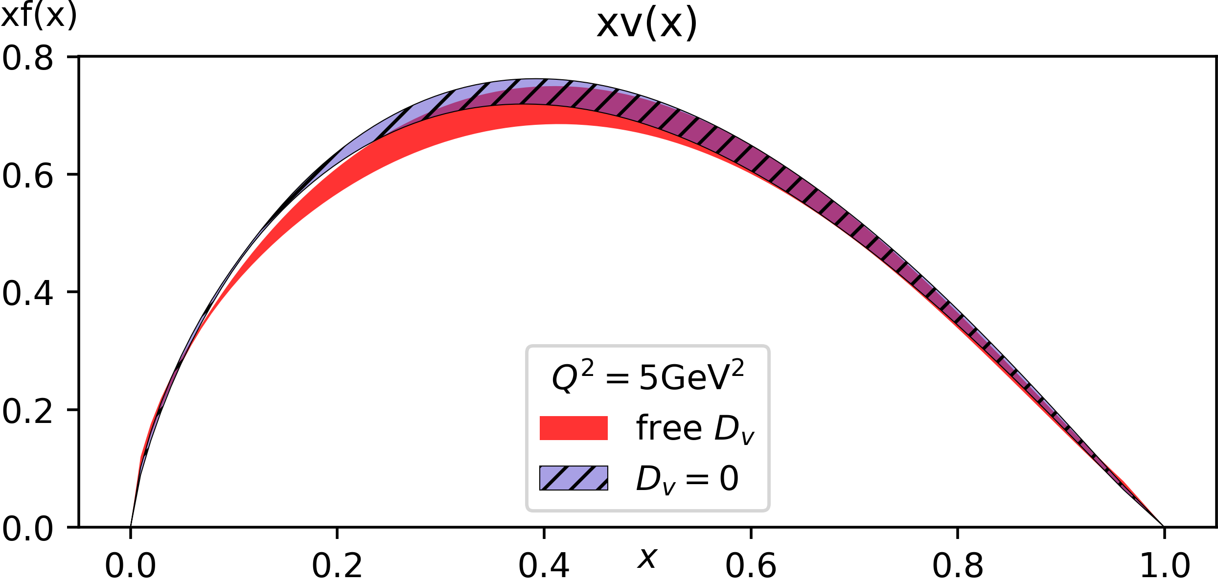
Figure 2: The valence distribution when using minimal parameterisation ($D_{v}=0$) and the extended parameterisation with free $D_{v}$. The shown uncertainty bands do not include scale variations.

In the case of prompt photon production, the contribution of fragmentation photons cannot be accounted for using the described techniques. The model used in the fit included only the direct photons. We estimate the impact of the missing fragmentation contribution by comparing the total integrated cross-sections computed using MCFM for proton-proton collision at the WA70 energy with and without fragmentation. The relative difference of $32\%$ is treated as the theoretical uncertainty in overall normalization of the WA70 data. In the run without fragmentation, Frixione isolation is used. In the other run the fragmentation function set GdRG__LO and cone isolation are used. The isolation cone size parameter is $R_{0}=0.4$ for both cases.

IV Statistical treatment and estimation of uncertainties

The PDF parameters are found by minimizing the $\chi^{2}$ function defined as

$$\chi^{2}=\sum_{i}\frac{(d_{i}-\tilde{t}_{i})^{2}}{\left(\delta^{\text{syst}}_{i}\right)^{2}+\left(\sqrt{\frac{\tilde{t}_{i}}{d_{i}}}\delta^{\text{stat}}_{i}\right)^{2}}+\sum_{\alpha}b_{\alpha}^{2},$$ (3)

where $i$ is the index of the datapoint and $\alpha$ is the index of the source of correlated error. The measured cross-section is denoted by $d_{i}$, with $\delta^{\text{syst}}_{i}$ and $\delta^{\text{stat}}_{i}$ being respectively the corresponding systematic and statistical uncertainties. The $t_{i}$’s represent the calculated theory predictions, and $\tilde{t}_{i}=t_{i}\left(1-\sum_{\alpha}\gamma_{i\alpha}b_{\alpha}\right)$ are theory predictions corrected for the correlated shifts. $\gamma_{i\alpha}$ is the relative coefficient of the influence of the correlated error source $\alpha$ on the datapoint $i$, and $b_{\alpha}$ is the nuisance parameter for the correlated error source $\alpha$.

The error rescaling $\tilde{\delta}^{\text{stat}}=\sqrt{\frac{\tilde{t}_{i}}{d_{i}}}\delta^{\text{stat}}$ is used to correct for Poisson fluctuations of the data. Since statistical uncertainties are typically estimated as a square root of the number of events, a random statistical fluctuation down in the number of observed events leads to a smaller estimated uncertainty, which gives such points a disproportionately large weight in the fit. The error rescaling corrects for this effect. This correction was only used for the Drell-Yan data.

The nuisance parameters $b_{\alpha}$ are used to account for correlated uncertainties. In this analysis the correlated uncertainties consist of the overall normalization uncertainties of the datasets, the correlated shifts in predictions related to uncertainties from nuclear PDFs, and the strong coupling constant $\alpha_{S}(M_{Z}^{2})=0.118\pm 0.001$. The nuisance parameters are included in the minimization along with the PDF parameters. They determine shifts of the theory predictions and contribute to the $\chi^{2}$ via the penalty term $\sum_{\alpha}b_{\alpha}^{2}$. For overall data normalization, the coefficients $\gamma_{i\alpha}$ are relative uncertainties as reported by the corresponding experiments, and, in the case of the WA70 data, the abovementioned additional $32\%$ theoretical uncertainty, (listed in Table 2).

Table 2: The normalization and partial $\chi^{2}$ for the considered datasets. The normalization uncertainty is presented as estimated by corresponding experiments. In order to agree with theory predictions, the measurements must be multiplied by the normalization factor. Deviations from 1 in the normalization factor lead to a penalty in $\chi^{2}$, as described in Section IV.

Experiment	Normalization uncertainty	Normalization factor	$\chi^{2}/N_{\text{points}}$
E615	15 %	$1.160\pm 0.020$	$206/140$
NA10 $(194\ \text{GeV})$	6.4%	$0.997\pm 0.014$	$107/67$
NA10 $(286\ \text{GeV})$	6.4%	$0.927\pm 0.013$	$95/73$
WA70	32%	$0.737\pm 0.012$	$64/99$

For the uncertainties from nuclear PDFs and $\alpha_{S}$, the coefficients $\gamma_{i\alpha}$ are estimated as derivatives of the theory predictions with respect to $\alpha_{S}$ and the uncertainty eigenvectors of the nuclear PDFs as provided by the nCTEQ15 set. This linear approximation is valid only when the minimisation parameters are close to their optimal values. It was verified that this condition was satisfied for the performed fits.

The uncertainty of the perturbative calculation is estimated by varying the renormalization scale $\mu_{R}$ and factorization scale $\mu_{F}$ by a factor of two up and down, separately for $\mu_{R}$ and $\mu_{F}$. The scales were varied using APPLgrid, and the variations were coherent for all data bins. Renormalization scale variation for DGLAP evolution was not performed. We observe a significant dependence of the predicted cross-sections on $\mu_{R}$ and $\mu_{F}$: the change in predictions is $\sim 10\%$, which is comparable to the normalization uncertainty of the data. This dependence indicates that next-to-next-to-leading order corrections may be significant.

In order to estimate the uncertainty related to the flexibility of chosen parameterisation, the fit is repeated with a varied initial scale $Q_{0}^{2}=1.9\pm 0.4\ \text{GeV}^{2}$. This variation leads to only a small change in $\chi^{2}$ ($\Delta\chi^{2}\lesssim 1$). In order to stay below the charm mass, for variation up to $Q^{2}_{0}=2.3\ \text{GeV}^{2}$ the mass threshold $m_{c}^{2}$ was shifted up by the same amount. The effect of such a change in the charm mass threshold by itself was found to be negligible.

V Results

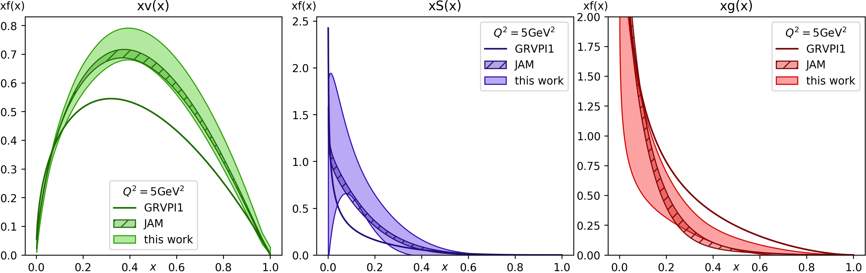
Figure 3: Comparison between the pion PDFs obtained in this work, a recent determination by the JAM collaborationBarry et al. (2018), and the GRVPI1 pion PDF setGluck et al. (1992).

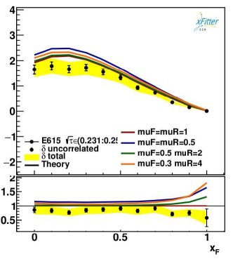
Figure 4: We display the scale variation of the cross section for a sample E615 $\sqrt{\tau}$ bin as a function of $x_{F}$. Note, the normalization factor of Table 2 ($1.60\pm 0.020$) has not been applied. We observe the relative impact of the scale variation is minimal except at very large $x$ ($x\gtrsim 0.9$).

Figure 3 shows the obtained pion PDFs in comparison to a recent analysis by JAMBarry et al. (2018), and to GRVPI1Gluck et al. (1992). The new valence distribution presented here is in good agreement with JAM, and both differ with the early GRV analysis. The relatively difficult to determine sea and gluon distributions are different in all three PDF sets, however, this new PDF and the JAM determination agree within the larger uncertainties of our fit.

In the case of valence distribution, the dominant contribution to the uncertainty estimate is the variation of the scales $\mu_{R}$ and $\mu_{F}$. For the sea and gluon distributions, the missing fragmentation contribution to prompt photon production is the dominant uncertainty source, and the effect of scale variation is also significant. Recall that JAM used the E615 and NA10 DY data (as we did), but used the HERA leading neutron electroproduction data while we used a direct photon analysis with a large normalization uncertainty (c.f., Table 2).

A comparison between experimental data and theory predictions obtained with the fitted PDFs is presented in Fig. 6. Reasonable agreement between data and theory is observed, with no systematic trends for any of the kinematic regions.

Table 3: Momentum fractions of the pion carried by the valence, sea and gluon PDFs at different scales $Q^{2}$ as determined in this work in comparison to other studies.

	$\langle xv\rangle$	$\langle xS\rangle$	$\langle xg\rangle$	$Q^{2}$ $(\text{GeV}^{2})$
JAMBarry et al. (2018)	$0.54\pm 0.01$	$0.16\pm 0.02$	$0.30\pm 0.02$	1.69
JAM (DY)	$0.60\pm 0.01$	$0.30\pm 0.05$	$0.10\pm 0.05$	1.69
this work	$0.55\pm 0.06$	$0.26\pm 0.15$	$0.19\pm 0.16$	1.69
Lattice-3Abdel-Rehim et al. (2015)	$0.428\pm 0.030$			4
SMRSSutton et al. (1992)	$0.47$			4
Han et al.Han et al. (2018)	$0.51\pm 0.03$			4
GRVPI1Gluck et al. (1992)	$0.39$	$0.11$	$0.51$	4
Ding et al.Ding et al. (2020b)	$0.48\pm 0.03$	$0.11\pm 0.02$	$0.41\pm 0.02$	4
this work	$0.50\pm 0.05$	$0.25\pm 0.13$	$0.25\pm 0.13$	4
JAM	$0.48\pm 0.01$	$0.17\pm 0.01$	$0.35\pm 0.02$	5
this work	$0.49\pm 0.05$	$0.25\pm 0.12$	$0.26\pm 0.13$	5
Lattice-1Best et al. (1997)	$0.558\pm 0.166$			5.76
Lattice-2Detmold et al. (2003)	$0.48\pm 0.04$			5.76
this work	$0.48\pm 0.05$	$0.25\pm 0.12$	$0.27\pm 0.13$	5.76
WRHWijesooriya et al. (2005)	$0.434\pm 0.022$			27
ChQM-1Nam (2012)	$0.428$			27
ChQM-2Watanabe et al. (2018)	$0.46$			27
this work	$0.42\pm 0.04$	$0.25\pm 0.10$	$0.32\pm 0.10$	27
SMRSSutton et al. (1992)	$0.49\pm 0.02$			49
this work	$0.41\pm 0.04$	$0.25\pm 0.09$	$0.34\pm 0.09$	49

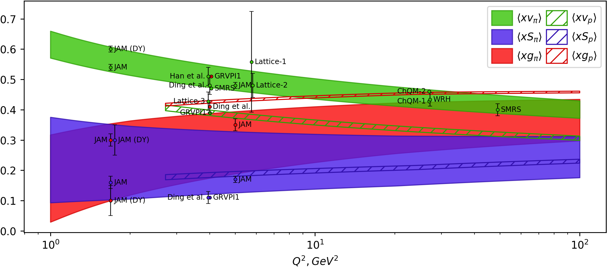
Figure 5: Momentum fractions of the pion as a function of $Q^{2}$. The error bands include all uncertainties described in Section IV. Analogous momentum fractions in the proton PDF set NNPDF31_nlo_as_0118 are shown for comparison. The labeled green, red, and blue points show respectively valence, sea, and gluon momentum fractions as reported by other studies. The references and numerical values for these points are listed in Table 3.

We now examine the high-$x$ behavior of the valence PDF. The asymptotic limit of the valence PDF as $x\to 1$ has been studied extensively in the literature. For example, Nambu-Jona-Lasinio modelsHolt and Roberts (2010) favor a $v(x)\sim(1-x)$ behavior while approaches based on the Dyson-Schwinger equations (DSE)Shi et al. (2018); Bednar et al. (2018) obtain a very different $v(x)\sim(1-x)^{2}$. The discrepancy between DSE predictions and fits to pion Drell-Yan data is well-knownWijesooriya et al. (2005); Aicher et al. (2010); Bednar et al. (2018), and it has been demonstrated that soft-gluon threshold resummation (which was not included in this analysis) may be used to account for this disagreementAicher et al. (2010). Alternatively, DSE calculations using inhomogeneous Bethe-Salpeter equationsBednar et al. (2018) can produce PDFs consistent with the linear behavior of the $v(x)$ in the region covered by DY data, pushing the onset of the $(1-x)^{2}$ regime to very high $x$.

Although the asymptotic behavior of the valence PDF is a theoretically interesting measurement, we will explain in the following why we are unable to determine this with the current analysis; conversely, details of the asymptotic region therefore do not impact our extracted pion PDFs.

First, the asymptotic DSE results only apply at asymptotically large $x$ values. While the precise boundary is a subject of debate, Ref. Bednar et al. (2018) demonstrates that the perturbative QCD predictions may only set in very near $x=1$; hence, the observed $(1-x)^{1}$ behavior could be real where the data exists. Consequently, it is entirely possible to have $(1-x)^{1}$ behavior at intermediate to large $x$, but then still find $(1-x)^{2}$ asymptotically. Except for the threshold-resummed calculation of Ref. Aicher et al. (2010), the fits to the E615 and NA10 dataConway et al. (1989); Betev et al. (1985); Stirling and Whalley (1993); Gluck et al. (1998, 1999); Barry et al. (2018) generally obtain high-$x$ behaviors that are closer to $(1-x)^{1}$ than the DSE result. This explains how these many fits can coexist with the asymptotic DSE limit.

What would it take to be able to accurately explore the $x\to 1$ asymptotic region? This region is challenging both experimentally and theoretically. On the experimental side, in the limit $x\to 1$ the PDFs are rapidly decreasing. Hence the cross section is very small, making large $x$ measurements difficult. Fig. 6 displays the full set of data we fit, and it is evident that the number of data at the largest $x_{F}$ values is limited. The issues on the theoretical side are also complex. In Fig. 4 we present the scale dependence for a sample subset of the E615 data. We see the relative scale dependence across the $x_{F}$ kinematic range is generally under control, with the exception of the very large $x_{F}$ limit; hence, the theoretical uncertainties of the NLO calculation increase precisely in the region required to extract the asymptotic behavior. Therefore, we reiterate that this analysis does not possess sufficient precision to infer definitive conclusions on the asymptotic $x\to 1$ limit of the pion structure function.

Furthermore, to properly study the $x\to 1$ asymptotic limit, a more sophisticated parametric form is required. The polynomial form for the pion valence PDF of Eq. 1 has only two or three free parameters $\{B_{v},C_{v},D_{v}\}$, and the large $x$ behavior is dominantly controlled by the $C_{v}$ coefficient. In light of the results of Ref. Bednar et al. (2018), a more flexible parameterization is required to accommodate separate $x$-dependence at both intermediate to large $x$ and then the asymptotic region.

The threshold resummation calculationLaenen et al. (2001) has generated significant interest, in part, because the resulting pion PDFs had a valence structure closer to the DSE $(1-x)^{2}$ form.Aicher et al. (2010) However it is important to recall that the PDFs themselves are not physical observables, but depend fundamentally on the underlying schemes and scales used for the calculation. If scheme-dependent PDFs are used with properly matched scheme-dependent hard cross sections, the result will yield scheme-independent observables as in Fig. 6. Additionally, were we to perform our analysis with the threshold resummed scheme, it would be most appropriate to do this for all the processes including both the DY and direct photon processes; however PDFs obtained with resummation corrections would also require resummed hard cross sections for the predictions. In contrast, our NLO analysis effectively absorbs resummation corrections (approximately) into the PDFs; but, it can be used to predict cross sections at NLO for future experiments using existing NLO open source tools.

To study the restrictions of our parameterization, we introduce an addition parameter $D_{v}$ for our valence PDF. This term has an impact on the intermediate to large $x$ behavior as evidenced by the change on the $C_{v}$ parameter, c.f, Table 1. However the improvement in the $\chi^{2}/N_{DoF}$ is minimal (1.19 vs 1.18), as is the $x$-dependence as shown in Fig. 2.

Fig. 5 shows the obtained momentum fractions in the pion as a function of $Q^{2}$. Recall that $A_{S}$ is a fit variable and $\{A_{v},A_{g}\}$ are determined by the sum rules of Eq.(2). Above the charm and bottom mass thresholds ($Q>m_{c},m_{b}$), the $c$ and $b$ quarks and anti-quarks are included in the sea distribution. For comparison, we have overlaid the results from the other studies listed in Table 3; these results are consistent within our uncertainties, except for the lattice simulation of Ref. Abdel-Rehim et al. (2015) (denoted by label ”Lattice-3”) and the GRVPI1 set.

Additionally, we have displayed the proton momentum fractions for the NNPDF31_nlo_as_0118Ball et al. (2017) set. Relative to the proton, we find the valence of the pion is larger, the gluon is smaller, and the sea component is similar, within uncertainties. We also note the $Q^{2}$-dependence of the various components are similar for both the pion and the proton, as they are all determined by the same DGLAP evolution equations.

VI Summary and outlook

We have presented the first open-source analysis of pion PDFs. We have used Drell-Yan and prompt photon production data with APPLgrids generated from MCFM to extract the PDFs at NLO. Additionally, we have performed a complete analysis of both experimental and theoretical uncertainties including renormalization and factorization scale variation ($\mu_{R},\mu_{F}$), strong coupling variation ($\alpha_{S}$), and PDFs (both proton and nuclear).

Comparing with other pion PDFs from the literature, our results are similar to JAM, but differ from the GRVPI1 set. Although the valence distribution is comparably well constrained, the considered data are not sensitive enough to unambiguously determine the sea and gluon distributions. We note our uncertainties are larger than JAM due to i) the theoretical uncertainties discussed above, and ii) the large normalization uncertainty on our direct photon analysis (JAM uses LN electroproduction instead). This is an area where new data, such as $J/\Psi$ production, could play an important role in constraining the gluon.Chang et al. (2020)

The data are reasonably well-described by NLO QCD, but the sensitivity to $\mu_{R}$ and $\mu_{F}$ indicates that next-to-next-to-leading order corrections could be significant, especially in the very large $x$ region; this precludes us from extracting the asymptotic behavior of the valence distribution.

We will provide the extracted pion PDFs in the LHAPDF6 PDFs library, and the APPLgrid grid files in the PloughsharePlo grid library. Since xFitter is an open-source program, it provides the community with a versatile tool to study meson PDFs which can be extended to perform new analyses. In particular, when data from future experiments, such as COMPASS++/AMBER,[50] becomes available, studying more flexible parameterization forms and including corrections beyond NLO will be of interest.

Figure 6: Considered experimental data and corresponding theory predictions. The displayed theory predictions include correlated shifts. Bands of different colors correspond to different datasets. Width of the bands shows uncertainty of the theory predictions. The cross-sections are shown in the same format as adopted by corresponding experimental papers. The E615 data is given as $\textrm{d}^{2}\sigma/(\textrm{d}\sqrt{\tau}\textrm{d}x_{F})$ in nb/nucleon, averaged over each $(\sqrt{\tau},x_{F})$ bin. The DY data from the NA10 experiment is $\textrm{d}^{2}\sigma/(\textrm{d}\sqrt{\tau}\textrm{d}x_{F})$ in nb/nucleus, integrated over each $(\sqrt{\tau},x_{F})$ bin. The WA70 data on direct photon production is given as invariant cross-section $E\textrm{d}^{3}\sigma/\textrm{d}p^{3}$ in pb, averaged over each $(p_{T},x_{F})$ bin.