The Aarhus red giants challenge II

Abstract

Context. The large quantity of high-quality asteroseismic data that have been obtained from space-based photometric missions and the accuracy of the resulting frequencies motivate a careful consideration of the accuracy of computed oscillation frequencies of stellar models, when applied as diagnostics of the model properties.

Aims. Based on models of red-giant stars that have been independently calculated using different stellar evolution codes, we investigate the extent to which the differences in the model calculation affect the model oscillation frequencies and other asteroseismic diagnostics.

Methods. For each of the models, which cover four different masses and different evolution stages on the red-giant branch, we computed full sets of low-degree oscillation frequencies using a single pulsation code and, from these frequencies, typical asteroseismic diagnostics. In addition, we carried out preliminary analyses to relate differences in the oscillation properties to the corresponding model differences.

Results. In general, the differences in asteroseismic properties between the different models greatly exceed the observational precision of these properties. This is particularly true for the nonradial modes whose mixed acoustic and gravity-wave character makes them sensitive to the structure of the deep stellar interior and, hence, to details of their evolution. In some cases, identifying these differences led to improvements in the final models presented here and in Paper I; here we illustrate particular examples of this.

Conclusions. Further improvements in stellar modelling are required in order fully to utilise the observational accuracy to probe intrinsic limitations in the modelling and improve our understanding of stellar internal physics. However, our analysis of the frequency differences and their relation to stellar internal properties provides a striking illustration of the potential, in particular, of the mixed modes of red-giant stars for the diagnostics of stellar interiors.

1 Introduction

Space-based photometric observations of oscillations in red-giant stars with the CoRoT (Baglin et al. 2013), Kepler (Borucki 2016) and, since 2018, the TESS (Ricker et al. 2014) missions have provided a huge set of accurate oscillation frequencies and other properties for these stars. These data provide the basis for detailed investigations of stellar structure and evolution, as well as the application of stellar properties in other areas of astrophysics, including the study of extra-solar planetary systems and the structure and evolution of the Galaxy. A necessary component of almost any analysis of such asteroseismic data is the use of modelling of stellar structure and evolution and the computation of oscillation frequencies for the resulting models. Given the complexity of stellar modelling, it is a non-trivial task to secure the required numerical and physical accuracy. Specifically, a full utilisation of the analysis of the observations requires that the numerical errors in the computed properties are substantially smaller than the uncertainties in the observations. Although adequate convergence of the computations can, to some extent, be tested by comparing results obtained with different numbers of meshpoints or timesteps in the models, more subtle errors in the calculations can probably only be uncovered through comparisons of the results of independent codes under carefully controlled conditions.

Extensive comparisons of this nature were organised for main-sequence stars in connection with the CoRoT project (Lebreton et al. 2008). Detailed comparisons between stellar models for the Red Giant Branch stage available in the literature have been discussed by Cassisi et al. (1998), Salaris et al. (2002), and Cassisi (2017). In the Aarhus Red Giant Challenge, we have so far concentrated on the numerical properties of the computation of the stellar models. Thus, the models are computed using, to the extent possible, the same input physics and basic parameters, and the comparisons are carried out at carefully specified stages in the evolution along the red-giant branch. Differences between the model properties, including their oscillation frequencies, should therefore reflect differences (and errors) in the numerical implementation of the solution of the equations of stellar evolution, or in the implementation of the physics. Also, we considered the effects of the resulting model differences on the computed oscillation frequencies, hence providing a link to the asteroseismic observations, with the goal of strengthening the basis for the analysis of the results of space-based photometry.

The initial analysis has focused on models up to and including the red-giant branch, emphasising the latter stage where energy production takes place in a hydrogen-burning shell around an inert helium core. Silva Aguirre et al. (2020, Paper I) presented model calculations for selected models with masses of $1$, $1.5$, $2$, and $2.5\,\mathrm{M}_{\odot}$ on the main sequence and the red-giant branch; the models analysed in detail were characterised in terms of radii chosen such that the models are of interest in connection with the asteroseismic investigations. The calculations used nine different stellar-evolution codes; Paper I discusses the differences between the results in terms of the overall properties of the models. The present paper considers oscillation calculations, using a single oscillation code, for the models presented in Paper I; this includes some discussion of the relation between the stellar structure and oscillation properties. A striking result is that the oscillation properties, in accordance with the potential for asteroseismic analyses, serve as a ‘magnifying glass’ on the differences in the stellar models, highlighting aspects where different codes yield results that are significantly different at the accuracy of the asteroseismic observations.

Further papers in this series will extend the analysis to the so-called clump (or horizontal-branch) stars where, in addition to the hydrogen-burning shell, there is helium fusion in the core; this leads to a rather complex structure and pulsation properties of the stars, with interesting consequences for the comparison between models and observed oscillations. In addition, we shall consider comparisons between models computed with ‘free physics’, where each modeller chooses the parameters and physical properties that would typically be used in the analysis of, for example, Kepler data. Finally, since the computation of stellar oscillations for these evolved models involves a number of challenges, an additional consideration of the comparisons between independent pulsation codes, for a number of representative models, is also planned.

2 Properties of red-giant oscillations

2.1 General properties

We consider oscillations of small amplitude and neglect effects of rotation and other departures from spherical symmetry. Then the modes depend on colatitude $\theta$ and longitude $\phi$ as spherical harmonics, $Y_{l}^{m}(\theta,\phi)$. Here the degree $l$ measures the total number of nodes on the stellar surface and the azimuthal order $m$ defines the number of nodal lines crossing the equator. Frequencies of spherically symmetric stars are independent of $m$. In addition, a mode is characterised by the number and properties of the nodes in the radial direction, which define the radial order $n$. For reviews of the properties of stellar oscillations see, for example, Aerts et al. (2010); Chaplin & Miglio (2013); Hekker & Christensen-Dalsgaard (2017); we discuss problems with the definition of the radial order in Section A.4.

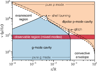
Figure 1: Characteristic frequencies $S_{l}/2\pi$ for $l=1$ and $2$ (dashed and dot-dashed; cf. Eq. 1) and $N/2\pi$ (solid; cf. Eq. 2) in the ASTEC $1\,\mathrm{M}_{\odot},7\,\mathrm{R}_{\odot}$ model. The horizontal red band marks the region around $\nu_{\rm max}$, the estimated frequency of maximum oscillation power (cf. Eq. 8), where observed modes are expected. The blue and orange areas indicate the corresponding regions of g- and p-mode behaviour, for $l=1$. The glitch in the buoyancy frequency is caused by the near-discontinuity in the hydrogen abundance resulting from the penetration, during the first dredge-up, of the convective envelope into a region where the composition has been modified by nuclear reactions (see also Paper I).

Radial modes, with $l=0$, are purely acoustic, that is, standing sound waves. Modes with $l>0$ in red giants all have a mixed character, behaving as acoustic modes in the outer parts of the star and as internal gravity waves in the core. This is controlled by two characteristic frequencies of the star: the acoustic (or Lamb) frequency

$$S_{l}={Lc\over r}\;,$$ (1)

and the buoyancy (or Brunt-Väisälä) frequency $N$, given by

$$N^{2}=g\left({1\over\Gamma_{1}}{{\rm d}\ln p\over{\rm d}r}-{{\rm d}\ln\rho\over{\rm d}r}\right)\;.$$ (2)

Here $L=\sqrt{l(l+1)}$, $c$ is adiabatic sound speed, $r$ is distance to the centre, $g$ is local gravitational acceleration, $p$ is pressure, $\rho$ is density, and $\Gamma_{1}=(\partial\ln p/\partial\ln\rho)_{\rm ad}$ is adiabatic compressibility, the derivative being at constant specific entropy. These frequencies are illustrated in Fig. 1 for a $1\,\mathrm{M}_{\odot},7\,\mathrm{R}_{\odot}$ model, together with the typical observed frequency range around the estimated frequency $\nu_{\rm max}$ at maximum oscillation power (see below; also Hekker & Christensen-Dalsgaard 2017). In the outer region, where $\nu>S_{l}$ and $\nu>N$ (i.e. the p-mode cavity), the mode behaves acoustically, while in the core where $\nu<S_{l}$ and $\nu<N$ (i.e. the g-mode cavity) the mode behaves like an internal gravity wave. In the intermediate region, the mode has an exponential behaviour; the extent of this so-called evanescent region controls the coupling between the acoustic and gravity-wave behaviour in the given mode. As a result of these properties, all nonradial modes, with $l>0$, have a mixed nature, with sensitivity both to the outer layers and to the core. For detailed discussions of such mixed modes see, for example, Hekker & Christensen-Dalsgaard (2017); Mosser et al. (2018); and references therein. Here we present some of the properties of the modes which are useful for the following analysis.

Acoustic modes of low degree have the following asymptotic behaviour (Shibahashi 1979; Tassoul 1980; Gough 1993):

$$\nu_{n_{\rm p}l}\approx\Delta\nu\left(n_{\rm p}+{l\over 2}+\epsilon_{\rm p}\right)+d_{n_{\rm p}l}\;,$$ (3)

for the cyclic frequencies $\nu_{n_{\rm p}l}$. Here the asymptotic expression for the large frequency separation $\Delta\nu$ is

$$\Delta\nu=\Delta\nu_{\rm as}=\left(2\int_{0}^{R_{*}}{{\rm d}r\over c}\right)^{-1}\;,$$ (4)

that is, the inverse of twice the sound travel time between the centre and the so-called acoustic surface (Houdek & Gough 2007), at a distance $R_{*}$ from the centre, in the stellar atmosphere. In the strict asymptotic analysis, $\epsilon_{\rm p}$ is a constant and the small higher-order effects are contained in $d_{n_{\rm p}l}$ (see also Mosser et al. 2013). Here, however, we adopt the formalism of Roxburgh & Vorontsov (2013) and regard $\epsilon_{\rm p}$ as a phase function depending on frequency but not on degree, determined by the properties of the near-surface layers (see also Christensen-Dalsgaard & Pérez Hernández 1992); this allows us to assume that $d_{n_{\rm p}l}$ is 0 for $l=0$. For the purely acoustic radial modes, Eq. (3) provides an approximation to the frequencies as a function of mode order $n_{\rm p}$; for the mixed nonradial modes the acoustically dominated modes (known as p-m modes) approximately satisfy the relation for an order $n_{\rm p}$ characterising the acoustic behaviour.

Observed and computed acoustic-mode frequencies follow Eq. (3) fairly closely, to leading order, although the value of the large frequency separation obtained from Eq. (4) is not sufficiently accurate to be applied to comparisons with observations. In the analysis of observed frequencies, various techniques can be used to determine the large frequency separation (e.g. Huber et al. 2009; Mosser & Appourchaux 2009; Hekker et al. 2010; Kallinger et al. 2010). The relation between different measures of the large frequency separation for stellar models was discussed by Belkacem et al. (2013) and Mosser et al. (2013). Here we follow White et al. (2011) and Mosser et al. (2013) and consider $\Delta\nu_{\rm fit}$ obtained from a weighted least-squares fit to frequencies of radial modes around the frequency $\nu_{\rm max}$ of maximum power (see Eq. 8 below), with a weight reflecting an estimate of the mode power. Some details on the fit are provided in Section A.3. We do note, however, that this procedure does not fully represent the weighting in the analyses of observational data, which are typically done directly from the observed power spectrum, for example through a cross-correlation analysis, without reference to the individual mode frequencies. Even so, obtaining $\Delta\nu_{\rm fit}$ from a fit to the computed frequencies provides a convenient way to compare the results for different codes.

Modes dominated by internal gravity waves require density variations over spherical surfaces in the star and are therefore only found for $l>0$. For such pure g modes, the periods $\Pi_{n_{\rm g}l}=1/\nu_{n_{\rm g}l}$ satisfy

$$\Pi_{n_{\rm g}l}=\Delta\Pi_{l}\left(n_{\rm g}+\epsilon_{\rm g}\right)$$ (5)

(e.g. Shibahashi 1979; Tassoul 1980), where

$$\Delta\Pi_{l}={\Pi_{0}\over L}\;,\qquad\Pi_{0}=2\pi^{2}\left(\int N{{\rm d}r\over r}\right)^{-1}\;,$$ (6)

the integral being over the gravity-wave cavity, and $\epsilon_{\rm g}$ is a phase, the so-called gravity offset, that may depend on $l$. Mixed modes dominated by the gravity-wave behaviour (the g-m modes) approximately satisfy Eq. (5), with $n_{\rm g}$ being an order characterising the g-mode behaviour (see also Fig. 2 below), and hence provide a measure of $\Delta\Pi_{l}$. However, additional important characteristics are provided by the measure $q$ of the coupling between the g- and p-mode cavities and $\epsilon_{\rm g}$, which provide information about the evanescent region and the upper part of the g-mode cavity (e.g. Takata 2016; Hekker & Christensen-Dalsgaard 2017; Pinçon et al. 2019).

2.2 Observational properties

The information available from the observed frequencies of oscillation depends strongly on the quality of the data. The most visible modes are the acoustically dominated (p-m) modes, which provide information about the overall properties of the star. They are characterised by the large frequency separation $\Delta\nu$ (cf. Eq. 4) and the frequency $\nu_{\rm max}$ of maximum power. It follows from homology scaling that, approximately, $\Delta\nu\propto\bar{\rho}^{1/2}$ where $\bar{\rho}$ is the mean density of the star. Specifically,

$$\Delta\nu\simeq\left({M\over\,\mathrm{M}_{\odot}}\right)^{1/2}\left({R\over\,\mathrm{R}_{\odot}}\right)^{-3/2}\Delta\nu_{\odot}\;,$$ (7)

valid for both $\Delta\nu_{\rm as}$ and $\Delta\nu_{\rm fit}$, where $\Delta\nu_{\odot}$ is the corresponding value for the Sun. A characteristic observed value is $\Delta\nu_{\odot}\simeq 135.1\,\mu{\rm Hz}$. Also, observationally (Brown et al. 1991) and with some theoretical support (Belkacem et al. 2011) $\nu_{\rm max}$ scales as the acoustic cut-off frequency, such that

$$\nu_{\rm max}\simeq{M\over\,\mathrm{M}_{\odot}}\left({R\over\,\mathrm{R}_{\odot}}\right)^{-2}\left({T_{\rm eff}\over T_{\rm eff,\odot}}\right)^{-1/2}\nu_{\rm max,\odot}\;,$$ (8)

where $\nu_{\rm max,\odot}\simeq 3090\,\mu{\rm Hz}$ is the frequency at maximum power for the Sun. In an extensive analysis of a large sample of Kepler red giants, Yu et al. (2018) found relative uncertainties in the large frequency separation $\Delta\nu$ below 0.1 %, in some cases, with a median value of 0.6 %, while the median uncertainty in $\nu_{\rm max}$ was 1.6 %. From the scaling relations in Eqs. (7) and (8), stellar masses and radii can be determined (see, for example, Kallinger et al. 2010; Yu et al. 2018). In practice, departures from the strict scaling relations, for example caused by departures from homology, need to be taken into account (see Hekker 2019, for a review); we return to this below in connection with a discussion of the scaling in Eq. (7).

The g-m modes, with a large component of internal gravity wave, provide strong constraints on stellar properties (for an early example, see Hjørringgaard et al. 2017). With improved analysis, further details on the g-m mode properties are becoming available (Mosser et al. 2018), providing further constraints on the stellar internal properties. Uncertainties in individual frequencies for both acoustic and mixed modes are as low as $0.01\,\mu{\rm Hz}$ (Corsaro et al. 2015; de Montellano et al. 2018), corresponding to relative uncertainties of order $10^{-4}$. Analysis of observed data on mixed modes in red giants has so far mainly been carried out in terms of determinations of the asymptotic properties characterised by $\Delta\Pi_{l}$, $q$ and $\epsilon_{g}$ as obtained from fitting a full asymptotic expression to the observed frequencies. (e.g. Bedding et al. 2013; Mosser et al. 2014, 2017, 2018). Uncertainties in the dipolar period spacing $\Delta\Pi_{1}$ of around $0.1\,{\rm s}$ were quoted by Hekker et al. (2018); Mosser et al. (2018). Detailed model fits to individual frequencies should also be feasible but have so far apparently not seen much use.

2.3 Oscillation properties of red-giant models

Figure 2: Top: Mode inertia (cf Eq. 9) for modes of degree $l=0$ (solid line, circles), $1$ (dashed line, triangles), and $2$ (dot-dashed line, squares), in the ASTEC $1\,\mathrm{M}_{\odot},7\,\mathrm{R}_{\odot}$ model. Bottom: Separation between periods of adjacent modes with $l=1$ in this model, plotted against frequency. The horizontal dashed line shows the asymptotic period spacing $\Delta\Pi_{1}=\Pi_{0}/\sqrt{2}$ (cf. Eqs. 5 and 6). The heavy vertical dotted lines show the frequency interval where power is half its maximum value, according to the fit of Mosser et al. (2012) (see also Section A.3).

To compare the oscillation properties of the models involved in the challenge the equations of adiabatic oscillations were solved using the code ADIPLS (Christensen-Dalsgaard 2008a). This code was compared in detail with other pulsation codes by Moya et al. (2008) and, more recently as part of the present project, with the GYRE code (Townsend & Teitler 2013). Owing to the condensed core of red-giant stars and the resulting very high value of the buoyancy frequency, modes of very high radial order are involved, requiring some care in the preparation of the models for the oscillation calculations; some details of these procedures are discussed in Section A.1; in Section A.2 we estimate the numerical errors in the resulting frequencies, both the intrinsic errors of the oscillation calculation and the effects on the frequencies from the errors in the computation of the ASTEC models, which are used for reference in the comparisons. Comparisons between models should be carried out at fixed mode order, requiring a determination of the order of the computed modes. For dipolar modes, this gives rise to some complications, compounded by inconsistencies in the structure very near the centre in some models, as discussed in Section A.4. Computed frequencies for all models, as well as the model structure, are provided at the website of the project.

To characterise the properties of the modes a very useful quantity is the normalised mode inertia,

$$E={\int_{V}\rho|\delta\kern-4.49997pt\delta\kern-4.49997pt\delta\mbox{\boldmath$r$}|^{2}{\rm d}V\over M|\delta\kern-4.49997pt\delta\kern-4.49997pt\delta\mbox{\boldmath$r$}|^{2}_{\rm phot}}\;,$$ (9)

where $\delta\kern-4.49997pt\delta\kern-4.49997pt\delta\mbox{\boldmath$r$}$ is the displacement vector and ‘phot’ indicates the photospheric value, defined at the location where the temperature equals the effective temperature; the integral is over the volume $V$ of the star. In Fig. 2 the top panel shows the inertia for a $1\,\mathrm{M}_{\odot},7\,\mathrm{R}_{\odot}$ model computed with ASTEC. Predominantly acoustic (p-m) modes have their largest amplitude in the outer layers of the star, where $\rho$ is small, and hence $E$ is relatively small, while g-m modes have large inertias. For the radial modes, the inertia decreases strongly with increasing frequency at low frequency, while it is almost constant at higher frequency. For $l=1$ and $2$, there is evidently a very high density of modes, most of which have inertia much higher than those of the radial modes and hence are predominantly of g-m character. However, there are clear acoustic resonances where the inertia approaches the radial-mode values and the modes are predominantly of p-m character. The frequencies of these resonances satisfy the asymptotic relation in Eq. (3); in particular, $l=0$ and $2$ modes separated by one in the acoustic order $n_{\rm p}$ have frequencies at a small separation determined by the term in $d_{n_{\rm p}l}$. It should also be noticed that the minimum inertia at the resonances is substantially lower for $l=2$ than for $l=1$: as shown in Fig. 1 the evanescent region is broader for $l=2$, leading to a weaker coupling and hence to a more dominant acoustic character of the mode at a resonance.

This mixed character of the modes is also visible in the bottom panel of Fig. 2, which shows the period spacing between adjacent dipolar modes in the same model. For most of the modes, particularly at low frequency, the computed period spacing is very close to the asymptotic value, indicated by the horizontal dashed line. However, at the acoustic resonances where the modes take on a p-m character the period spacing is strongly reduced; we note that these resonances take place at frequencies approximately satisfying Eq. (3).

3 Results of model comparisons

3.1 Stellar models

We computed oscillation properties of the models highlighted in Paper I. We note in particular that two sets of models have been considered. In one (in the following the solar-calibrated models), the mixing-length parameter $\alpha_{\rm MLT}$ was adjusted in each code to achieve a photospheric radius of $6.95508\times 10^{8}\,{\rm m}$ at the age of 4.57 Gyr of main-sequence evolution for the $1\,\mathrm{M}_{\odot}$ model. In the second (in the following the RGB-calibrated models), $\alpha_{\rm MLT}$ was fixed for each track by requiring a specific effective temperature $T_{\rm eff}$ for the $7\,\mathrm{R}_{\odot}$ models on the $1$ and $1.5\,\mathrm{M}_{\odot}$ tracks and the $10\,\mathrm{R}_{\odot}$ models on the $2$ and $2.5\,\mathrm{M}_{\odot}$ tracks. In the present section, we generally focus on the solar-calibrated models; results for the RGB-calibrated models are provided in Appendix B.

The following evolution codes were used:

• ASTEC: the Aarhus STellar Evolution Code; see Christensen-Dalsgaard (2008b).

• BaSTI: Bag of Stellar Tracks and Isochrones; see Pietrinferni et al. (2013).

• CESAM2k: Code d’Evolution Stellaire Adaptatif et Modulaire, 2000 version; see Morel & Lebreton (2008).

• GARSTEC: the GARching STellar Evolution Code; see Weiss & Schlattl (2008).

• LPCODE: the La Plata stellar evolution Code; see Miller Bertolami (2016).

• MESA: Modules for Experiments in Stellar Astrophysics, version 6950; see Paxton et al. (2013).

• MONSTAR: the Monash version of the Mt Stromlo evolution code; see Constantino et al. (2015).

• YaPSI: the Yale Rotational stellar Evolution Code, as used in the Yale-Potsdam Stellar Isochrones; see Spada et al. (2017).

• YREC: the Yale Rotating stellar Evolution Code; see Demarque et al. (2008).

We note that in order to avoid effects of different extents of the atmosphere in models from different codes for a given set of parameters, the models were truncated in the atmosphere at a height corresponding to the code with the smallest atmospheric extent, for the given case.

Further details about the codes and the models are provided in Paper I.

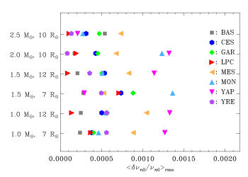
Figure 3: Root-mean-square relative differences, in the solar-calibrated case, in radial-mode frequencies relative to the ASTEC results, in the sense (model) - (ASTEC); the different codes are identified by the symbol shape and colour and labelled by the abbreviated name of the code: BAS (BaSTI), CES (CESAM), GAR (GARSTEC), LPC (LPCODE), MES (MESA), MON (MONSTAR), YAP (YaPSI), and YRE (YREC).

Table 1: Large frequency separations $\Delta\nu_{\rm fit}$ in $\,\mu{\rm Hz}$ obtained from fits to radial-mode frequencies as functions of mode order (cf. Eq. 3 and Section A.3) for solar-calibrated models.

$M/\,\mathrm{M}_{\odot}$	$R/\,\mathrm{R}_{\odot}$	ASTEC	BaSTI	CESAM	GARSTEC	LPCODE	MESA	MONSTAR	YAP	YREC
1.0	7.0	7.087	7.093	7.100	7.089	7.090	7.077	7.084	7.100	7.090
1.0	12.0	3.130	3.133	3.137	3.131	3.130	3.124	3.128	3.137	3.131
1.5	7.0	8.780	8.783	8.799	8.774	8.789	8.768	8.762	8.778	8.785
1.5	12.0	3.876	3.879	3.884	3.876	3.875	3.869	3.873	3.882	3.876
2.0	10.0	5.949	5.952	5.958	5.949	5.951	5.940	5.938	5.938	5.948
2.5	10.0	6.739	6.746	6.744	6.735	6.737	6.726	6.736	6.744	6.738

3.2 Acoustic properties

We first consider the properties of the acoustically-dominated oscillations, as characterised by the radial modes. As an indication of the frequency differences between different codes, Fig. 3 shows the root-mean-square relative differences in radial-mode frequencies between the various codes and ASTEC, including all modes up to the acoustic cut-off frequency. We note that they are far bigger than the observational uncertainties of the individual frequencies (cf. Section 2.2).

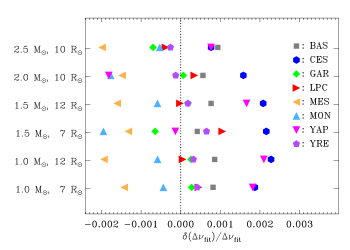
Figure 4: Relative differences for solar-calibrated models in the large frequency separations $\Delta\nu_{\rm fit}$ obtained from fits to the radial-mode frequencies as functions of mode order (cf. Section A.3), compared with the ASTEC results, in the sense (model) – (ASTEC); the different codes are identified by the symbol shape and colour (cf. caption to Fig. 3).

The large frequency separation between acoustic modes is an important asteroseismic diagnostics. As discussed in Section 2.1, we characterise the observable values by the result $\Delta\nu_{\rm fit}$ of fitting the computed radial-mode frequencies to Eq. (3), representing $\epsilon_{\rm p}$ by a quadratic expression in mode order (cf. Section A.3). Table 1 provides values obtained from these fits in the solar-calibrated case, and Fig. 4 shows relative differences for these fitted values, relative to the ASTEC models. In most cases the relative differences are below 0.2 %, comparable with or somewhat bigger than the observational uncertainties of around 0.1 % (cf. Section 2.2).

Table 2: Correction factors $f_{\Delta\nu}$ (cf. Eq. 10) between the large frequency separation $\Delta\nu_{\rm fit}$ obtained from a fit to radial-mode frequencies and the value obtained from homology scaling for solar-calibrated models.

$M/\,\mathrm{M}_{\odot}$	$R/\,\mathrm{R}_{\odot}$	ASTEC	BaSTI	CESAM	GARSTEC	LPCODE	MESA	MONSTAR	YAP	YREC
1.0	7.0	0.9655	0.9661	0.9667	0.9658	0.9660	0.9656	0.9656	0.9682	0.9658
1.0	12.0	0.9572	0.9578	0.9588	0.9575	0.9573	0.9568	0.9571	0.9601	0.9573
1.5	7.0	0.9767	0.9769	0.9782	0.9761	0.9777	0.9768	0.9752	0.9774	0.9771
1.5	12.0	0.9677	0.9682	0.9691	0.9679	0.9677	0.9676	0.9676	0.9702	0.9677
2.0	10.0	0.9786	0.9789	0.9795	0.9787	0.9789	0.9786	0.9773	0.9777	0.9783
2.5	10.0	0.9915	0.9923	0.9917	0.9909	0.9912	0.9911	0.9915	0.9932	0.9911

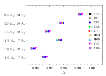
Figure 5: Correction factor $f_{\Delta\nu}$, for solar-calibrated models, in the scaling relation for the large frequency separation $\Delta\nu_{\rm fit}$ obtained from fits to the radial-mode frequencies (cf. Eq. 10). The different codes are identified by the symbol shape and colour (cf. caption to Fig. 3), with the addition of AST (for ASTEC).

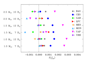
Figure 6: Differences relative to the ASTEC model in the solar-calibrated case, in the sense (model) – (ASTEC), in the correction factors $f_{\Delta\nu}$ (cf. Eq. 10) relating the large frequency separation $\Delta\nu_{\rm fit}$ obtained from a fit to radial-mode frequencies and the value obtained from homology scaling. The different codes are identified by the symbol shape and colour (cf. caption to Fig. 3).

The scaling relation in Eq. (7) is fundamental in the analysis of global seismic observations, but the underlying assumed homology scaling is not exact. Thus, it is often corrected by including a factor $f_{\Delta\nu}$ on the right-hand side (e.g. White et al. 2011; Rodrigues et al. 2017); (see Sharma et al. 2016, for an application). Within the present model analysis we replace Eq. (7) by

$$\Delta\nu_{\rm fit}=f_{\Delta\nu}\left({M\over\,\mathrm{M}_{\odot}}\right)^{1/2}\left({R\over\,\mathrm{R}_{\odot}}\right)^{-3/2}\Delta\nu_{\rm fit}^{\rm(cal)}\;,$$ (10)

where $\Delta\nu_{\rm fit}^{\rm(cal)}$ is the large separation resulting from a fit to the radial modes of the $(1\,\mathrm{M}_{\odot},1\,\mathrm{R}_{\odot})$ models used to calibrate the mixing length in the solar-calibrated case. The resulting values of the correction factor $f_{\Delta\nu}$ are shown in Table 2 and Fig. 5 for the solar-calibrated case. The dominant variation is that $f_{\Delta\nu}$ approaches unity for the most massive model, in accordance with the results obtained by Guggenberger et al. (2017); Rodrigues et al. (2017). Differences in $f_{\Delta\nu}$ between the different codes relative to ASTEC are shown in Fig. 6. We note that for any given model case there is a spread of around $\pm 0.002$ between the values of $f_{\Delta\nu}$ obtained by the different evolution codes. As pointed out by, for example, Sharma et al. (2016) the radius and mass obtained from direct scaling analysis of global asteroseismic observables scale as, respectively, $f_{\Delta\nu}^{-2}$ and $f_{\Delta\nu}^{-4}$. Thus, the spread between the codes would correspond to variations of around 0.4 and 0.8 % in the inferred radii and masses, when using Eq. (10) to analyse observed data.

Table 3: Frequency $\nu_{\rm max}$, in $\,\mu{\rm Hz}$, of maximum oscillation power estimated from Eq. (8) for solar-calibrated models.

$M/\,\mathrm{M}_{\odot}$	$R/\,\mathrm{R}_{\odot}$	ASTEC	BaSTI	CESAM	GARSTEC	LPCODE	MESA	MONSTAR	YAP	YREC
1.0	7.0	69.76	69.97	70.03	69.93	69.74	69.61	69.90	69.87	69.78
1.0	12.0	24.29	24.36	24.38	24.36	24.29	24.24	24.34	24.33	24.30
1.5	7.0	102.57	102.85	102.91	102.82	102.55	102.35	102.80	102.73	102.61
1.5	12.0	35.76	35.86	35.88	35.85	35.75	35.69	35.83	35.82	35.77
2.0	10.0	67.05	67.24	67.27	67.24	67.06	66.93	67.21	67.17	67.06
2.5	10.0	82.64	82.85	82.92	82.88	82.65	82.49	82.82	82.79	82.65

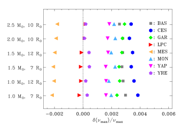
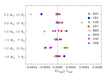
Figure 7: Relative differences in the estimated frequency $\nu_{\rm max}$ of maximum power, compared with the ASTEC results, in the sense (model) - (ASTEC); the different codes are identified by the symbol shape and colour (cf. caption to Fig. 3). The left panel shows results for the solar-calibrated models, and the right panel for the RGB-calibrated models (note the different scales on the abscissas).

The frequency $\nu_{\rm max}$ of maximum power plays an important role for asteroseismic inference. In view of this, we include a brief analysis of the differences in $\nu_{\rm max}$ between the models, even though these differences essentially reflect the differences in $T_{\rm eff}$, already discussed in Paper I, given that the comparison is carried out at fixed target model radius, and with a constraint on $GM/R^{3}$. Table 3 shows values of $\nu_{\rm max}$, estimated from Eq. (8), for solar-calibrated models, while Fig. 7 shows relative differences in $\nu_{\rm max}$, compared with the ASTEC values for both solar- and RGB-calibrated models. For the solar-calibrated models, there is a spread of order 50 K between different codes for any given model, corresponding to roughly 1 % (cf. Figs. 2 and 7, and Tables C.2 – C.4, of Paper I; see also Fig. 12 below). For the RGB-calibrated models, where $T_{\rm eff}$ was explicitly constrained on the RGB, the spread is less than 4 K, or 0.1 %. Thus, the differences are smaller by about an order of magnitude for the RGB-calibrated models. We note, however, that in either case the differences in $\nu_{\rm max}$ are far smaller than the typical observational uncertainty of 1.6 % (Yu et al. 2018) in this quantity.

Although the asymptotic value, $\Delta\nu_{\rm as}$, of the large frequency separation (cf. Eq. 4) does not provide sufficient accuracy for comparison with observed frequencies, it is still an interesting diagnostics of the acoustic properties of the models. We analyse it in Appendix C.

3.3 Mixed modes

Table 4: Asymptotic dipolar g-mode period spacings $\Delta\Pi_{1}$ in s (cf. Eq. 6) for solar-calibrated models.

$M/\,\mathrm{M}_{\odot}$	$R/\,\mathrm{R}_{\odot}$	ASTEC	BaSTI	CESAM	GARSTEC	LPCODE	MESA	MONSTAR	YAP	YREC
1.0	7.0	72.12	72.07	72.58	72.41	72.64	72.69	73.23	76.64	73.14
1.0	12.0	58.36	58.00	58.39	58.44	58.47	58.61	59.02	60.86	58.97
1.5	7.0	69.90	69.86	70.34	70.20	70.48	70.75	71.13	74.48	71.05
1.5	12.0	57.29	56.94	57.43	57.35	57.30	57.48	57.87	59.47	57.90
2.0	10.0	78.72	79.02	78.36	77.18	78.14	76.99	79.57	82.26	79.02
2.5	10.0	123.62	124.10	121.54	121.50	122.32	121.83	124.91	125.52	123.33

The asymptotic dipolar g-mode period spacing $\Delta\Pi_{1}=\Pi_{0}/\sqrt{2}$ (cf. Eqs. 5 and 6) are provided in Table 4 for solar-calibrated models, while the variations relative to the ASTEC models are shown in Fig. 8. Here relative differences of up to 2 – 4 % are found, corresponding to differences in $\Delta\Pi_{1}$ of several seconds, greatly exceeding the observational uncertainty of around 0.1 s (see Section 2.2). This reflects the sensitivity of the buoyancy frequency to the details of the core structure of the star, including the composition profile; we consider one example in some detail in Appendix F. The differences between the models illustrated in Fig. 8 generally arise from qualitatively similar, although generally smaller, model differences.

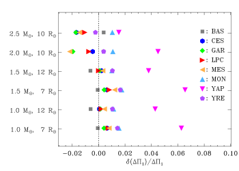
Figure 8: Relative differences for solar-calibrated models in the asymptotic period spacing $\Delta\Pi_{1}$, compared with the ASTEC results, in the sense (model) - (ASTEC); the different codes are identified by the symbol shape and colour (cf. caption to Fig. 3).

Figure 9: Relative differences in computed frequencies for the MESA solar-calibrated $1.5\,\mathrm{M}_{\odot},7\,\mathrm{R}_{\odot}$ model, compared with the ASTEC results, in the sense (MESA) - (ASTEC), for $l=0$ (open circles), $l=1$ (open triangles) and $l=2$ (filled squares). The differences are evaluated at fixed radial order.

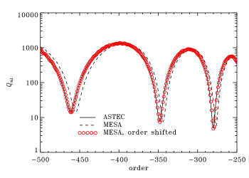
Figure 10: Scaled mode inertias for dipolar modes (with $l=1$) in the solar-calibrated ASTEC (solid) and MESA (dashed) $1.5\,\mathrm{M}_{\odot},7\,\mathrm{R}_{\odot}$ models, against mode order. The red circles show the MESA results, but shifted in order (see text).

As an example of the differences in individual frequencies, Fig. 9 compares frequencies of given radial order in the MESA model for $1.5\,\mathrm{M}_{\odot},7\,\mathrm{R}_{\odot}$ with ASTEC. The difference in the asymptotic frequency spacing is shown as a dashed line, and the dotted line shows the difference in the asymptotic period spacing, with inverted sign to convert relative period differences to frequency differences. In this case, the purely acoustic radial modes generally agree well between the two models, as does the asymptotic frequency spacing (see also Fig. 23). However, we note the increasing magnitude of the differences at the highest frequency that reflects issues with the modelling of the atmosphere in the MESA model (see Appendix D). The g-dominated nonradial modes have differences very close to the asymptotic value, while the more acoustically dominated modes have intermediate differences. Indeed, one would naively expect that the p-dominated nonradial modes would have frequency differences similar to the radial modes; instead, they are substantially higher in absolute value, with a clear nearly linear envelope for the most p-dominated cases.

The origin of this behaviour lies in the formally reasonable choice of comparing the modes at fixed radial order, regardless of the physical nature of the modes. In fact, modes with same order may have rather different physical nature. To analyse this, we consider the rescaled inertia $Q_{nl}=E_{nl}/\bar{E}_{0}(\nu_{nl})$ where $E$ was defined in Eq. (9) and $\bar{E}_{0}(\nu_{nl})$ is the radial-mode inertia interpolated to the frequency of the given mode. Figure 10 shows $Q_{nl}$ for $l=1$ against mode order for the two models. Here the p-dominated modes correspond to the dips in the curves, resulting from acoustic resonances. The resonances are largely fixed at the same frequency by the very similar acoustic behaviour of the MESA and ASTEC models, reflected in the close agreement in the radial-mode frequencies; however, it is obvious that they are shifted in mode order, as a result of the difference between the models in the period spacing and hence the relation between order and frequency. In other words, although the two models agree on the shape of the $Q_{nl}$ curve (including the location in frequency of the resonant dips), the mixed modes of the two models do not sample that curve at the same mode orders. As a result, a comparison at fixed order is between physically different modes, with a different weight to the p- and g-mode behaviour, in the vicinity of the acoustic resonances.

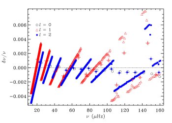
Figure 11: Relative differences in computed frequencies for the solar-calibrated MESA $1.5\,\mathrm{M}_{\odot},7\,\mathrm{R}_{\odot}$ model with suitable shifts in mode order (see text), compared with the ASTEC results, in the sense (MESA) - (ASTEC), for $l=0$ (black open circles), $l=1$ (red open triangles) and $l=2$ (blue filled squares). The larger pluses mark the p-dominated modes. The horizontal dotted line indicates zero difference.

From the point of view of comparing models and observations, the (formal) order is a somewhat inconvenient quantity since it is difficult to derive it directly from the observations, except with data of exceptionally high quality. Here the p-dominated modes are the natural starting points, anchoring the mode orders in the vicinity of an acoustic resonance. In the comparison of the model frequencies, this corresponds to shifting the mode orders of, say, the MESA model to obtain a new order $n^{\prime}$ such as to make the acoustic resonances occur at the same values of the order. As indicated by Fig. 10, the required shift decreases with increasing order. Thus, in the complete set $\{n^{\prime}\}$ of shifted orders there may be gaps or overlapping modes, but these can be arranged to occur near the maxima in $Q_{nl}$ where the modes are unlikely to be observed. As shown by the red circles in Fig. 10, with such a shift the behaviour of $Q_{nl}$ as a function of mode order is nearly indistinguishable between the models.

The effect of using the shifted orders in the frequency comparison at fixed order is illustrated in Fig. 11. Now the p-dominated modes, marked by larger pluses superposed on the symbols, do indeed have small frequency differences. This is particularly clear for the $l=2$ modes, where the coupling between the acoustic and gravity-wave regions is weaker and the p-dominated modes therefore have a cleaner acoustic nature.

To understand the behaviour shown in Fig. 11, we consider two models, Model 1 (the ASTEC model) and Model 2 (the MESA model), with period spacings $\Delta\Pi_{l}$ and $\Delta\Pi_{l}^{\prime}$. For simplicity, we assume that the g-mode phase shift $\epsilon_{\rm g}$ (cf. Eq. 5) is the same for the two models. We identify an acoustic resonance in Model 1, corresponding to the order $n_{0}$, and consider modes of order $n$ in Model 1 in the vicinity of $n_{0}$. To identify modes in Model 2 similarly close to the acoustic resonance, we choose a shift $k$ in order such that $\Delta\Pi_{l}(n_{0}+\epsilon_{\rm g})\simeq\Delta\Pi_{l}^{\prime}(n_{0}+k+\epsilon_{\rm g})$, or

$$k\simeq-{\delta\Delta\Pi_{l}\over\Delta\Pi_{l}^{\prime}}n_{0}\;,$$ (11)

where $\delta\Delta\Pi_{l}=\Delta\Pi_{l}^{\prime}-\Delta\Pi_{l}$, and compare modes with shifted mode order $n^{\prime}=n+k$ in Model 2 with modes of order $n$ in Model 1. From Eq. (11) it follows that the relative difference between the frequencies $\nu_{n^{\prime}l}^{\prime}$ and $\nu_{nl}$ of modes $(n^{\prime},l)$ and $(n,l)$ in Models 2 and 1 is

$${\nu_{n^{\prime}l}^{\prime}-\nu_{nl}\over\nu_{nl}} = -{\Pi_{n^{\prime}l}^{\prime}-\Pi_{nl}\over\Pi_{nl}}\simeq-\delta\Delta\Pi_{l}{n-n_{0}\over\Pi_{nl}}$$

$$\simeq -{\delta\Delta\Pi_{l}\over\Delta\Pi_{l}}{\Pi_{nl}-\Pi_{n_{0}l}\over\Pi_{nl}}\simeq{\delta\Delta\Pi_{l}\over\Delta\Pi_{l}}\left({\nu_{nl}\over\nu_{n_{0}l}}-1\right)\;,$$

where we neglected the difference between $\Delta\Pi_{l}^{\prime}$ and $\Delta\Pi_{l}$ in the denominator. Equation (6) shows that $\delta\Delta\Pi_{l}/\Delta\Pi_{l}$ is independent of $l$. Thus, according to Eq. (3.3) the frequency differences including the shift in mode order are linear functions of frequency with a slope depending on $\delta\Delta\Pi_{l}/\Delta\Pi_{l}$ and $\nu_{n_{0}l}$ but not on the degree, as is indeed found in Fig. 11.

The detailed frequency differences for other models or evolution codes are qualitatively similar, although reflecting the differences in global asteroseismic properties, in particular $\Delta\nu_{\rm as}$ and $\Delta\Pi_{1}$, as illustrated in Figs. 23 and 8. However, we note that these models to some extent reflect modifications to the modelling codes resulting from the analysis of earlier models. Earlier models, showing substantially larger deviations, provide interesting insight into the relation between the model structure and the resulting frequencies. We discuss examples of this in Appendices E and F.

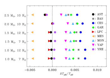
Figure 12: Relative differences in effective temperature $T_{\rm eff}$ between the RGB- and solar-calibrated models, in the sense (RGB-calibrated) – (solar-calibrated). The different codes are identified by the symbol shape and colour (cf. caption to Fig. 3).

3.4 The RGB-calibrated models

In Paper I, we showed that the effective temperature on the red-giant branch varied within a range of around 50 K between the solar-calibrated models. This variation is summarised in Fig. 12, which shows the differences between the effective temperatures in the RGB- and solar-calibrated models. (The differences are small for the ASTEC models, earlier versions of which were used to set the target values for the RGB calibration.) As discussed in Section 3.2, $T_{\rm eff}$ directly enters $\nu_{\rm max}$ and hence shows a much better agreement in the RGB- than in the solar-calibrated case (cf. Fig. 7); in particular, the differences in the latter case closely reflect the differences in $T_{\rm eff}$, shown in Fig. 12.

Other results for the RGB-calibrated modes are provided as tables and figures in Appendix B. A comparison between the various asteroseismic quantities between the RGB- and solar-calibrated cases (not illustrated) shows differences that are to some extent, but not completely, related to the differences in $T_{\rm eff}$ and are somewhat smaller than the differences between the different model calculations. Consequently, the variations between the codes in the RGB-calibrated case are qualitatively very similar to the variations discussed in the previous sections.

4 Discussion

The goal of the present project is to provide a secure basis for the analysis of observed frequencies of red-giant stars by identifying and eliminating errors and other uncertainties in the computation of stellar models and their frequencies. Paper I considered differences between different stellar evolution codes in the basic properties of stellar models, computed with tightly constrained parameters and physics. Here we address the corresponding properties of the oscillations of these models.

The errors in the computed frequencies include intrinsic errors in the frequency calculation, for a given stellar model. These are relatively easy to control, at least for the cases considered in the present investigation. The example illustrated in Fig. 14 indicates that the intrinsic numerical errors are well below the requirements imposed by current observations in the relevant frequency range for the oscillation code used here. Even so, there is a definite need for comparisons, planned in a future publication, between the results of independent oscillation calculations to detect possible systematic errors in the implementation of the oscillation equations in the codes.

A more important contribution to the errors in the computed frequencies is likely the error in the implementation and solution of the equations of stellar structure and evolution. The goal of the present investigation is to estimate these errors, by comparing results of stellar evolution calculations with independent codes using, as far as possible, the same physical assumptions (see Paper I). In fact, the analysis in the present project has identified, and led to the elimination of, a number of issues that have in some cases been present for many years in the codes that have taken part. Even so, following these corrections the results in Section 3 show that the model differences, reflecting potential errors in the modelling, in many cases do not yet match the constraints of the observational uncertainties. The estimates of $\nu_{\rm max}$ (cf. Table 3 and Fig. 7) agree substantially better than the relatively large observational uncertainty in this quantity. The differences in the large frequency separation $\Delta\nu_{\rm fit}$ obtained from fits to the radial-mode frequencies (cf. Table 1 and Fig. 4) are close to matching, or somewhat exceed, the accuracy of the observations. Finally, the root-mean-square differences of radial-mode frequencies (Fig. 3) are substantially bigger than the observational uncertainties in individual frequencies.

For the use of scaling relations based on acoustic modes, the correction factor $f_{\rm\Delta\nu}$ (cf. Eq. 10) is particularly important. The spread in $f_{\Delta\nu}$ of $\pm 0.2$ % between the different evolution codes (see Eq. 6) translate into variations of around 0.4 and 0.8 % in determinations of radius and mass from asteroseismic scaling relations, which are hardly insignificant.

Analyses of the properties of mixed modes provide detailed diagnostics of the deep interior of the star, owing to the sensitivity of the details of the acoustic resonances and the g-dominated modes. The analysis is often carried out in terms of fits of the frequencies to the asymptotic expression (e.g. Mosser et al. 2018), resulting in estimates of the g-mode period spacing $\Delta\Pi_{1}$, the quantity $q$ characterising the coupling between the g- and p-mode cavities and the gravity offset $\epsilon_{\rm g}$. Here we represented the effects of the model differences in terms of the asymptotic period spacing (cf. Eq. 6). A more detailed analysis in terms of a fit to the computed frequencies would have been interesting but is beyond the scope of this paper. However, a sample check for a single model case showed that the asymptotic period spacings are fully representative of the results based on period spacings obtained from such a fit. We note, on the other hand, that very interesting analyses of the information about stellar structure provided by $q$ and $\epsilon_{\rm g}$ were provided by Takata (2016); Pinçon et al. (2019).

The sensitivity of the computed asymptotic dipolar period spacings (cf. Table 4 and Fig. 8) to the detailed structure of the deep interior of the models is reflected in a substantial spread between the models, far bigger than the observational errors. In most cases, the relative differences are between $\pm 2$ %, with the YaPSI models showing somewhat bigger deviations. As a rough estimate we note from Table 4 that over the range $1-1.5\,\mathrm{M}_{\odot}$ in stellar mass, keeping the radius fixed at $7\,\mathrm{R}_{\odot}$, a change of one per cent in $\Delta\Pi_{1}$ corresponds on average to a change of more than $0.1\,\mathrm{M}_{\odot}$ in mass or a change in the inferred age of more than 30 %. Even though a model fit based solely on $\Delta\Pi_{1}$ is probably unrealistic, this estimate provides some indication of the effects of the uncertainties in stellar modelling on the asteroseismic inferences.

These differences in oscillation properties must reflect differences in the model structure, discussed in detail in Paper I, which arise despite the attempt to compute the models under identical assumptions; however, the connection is in most cases not immediately obvious. We analysed two examples in some detail. Appendix E considers differences in the acoustic-mode frequencies in the original GARSTEC models (cf. Fig. 27), which were found to be caused by differences in the implementation of the OPAL equation of state, illustrated in Fig. 28. Appendix F analyses the fairly substantial differences found in the asymptotic $\Delta\Pi_{1}$ and the g-m mode frequencies for the original LPCODE model with $2.5\,\mathrm{M}_{\odot}$, $10\,\mathrm{R}_{\odot}$. As discussed in detail in the appendix, this is related to differences in the hydrogen profile arising from a smaller main-sequence convective core in the LPCODE model, caused by inadequacies in the opacities. This deficiency has been corrected in the LPCODE results shown in Section 3, as perhaps the most dramatic of the many corrections to the modelling resulting from this challenge. It should be noted that the oscillation calculations act as a strong ‘magnifying glass’ on irregularities in the model structure, further motivating such improvements to the modelling; an example is discussed in Section A.4.

In the analysis of the results, we chose to emphasise the case of models where the mixing-length parameter was chosen based on the calibration of a $1\,\mathrm{M}_{\odot},1\,\mathrm{R}_{\odot}$ model (the so-called solar-calibrated case). This procedure matches the common practice of using such a calibration in general calculations of stellar models, including those that are used for asteroseismic fitting. From a physical point of view one might argue that the RGB-calibration, based on fixing the effective temperature on the red-giant branch, is more interesting since by doing this (at the assumed fixed radii) one also fixes the luminosity and hence important aspects of the internal structure of the stars. In fact, the results for the two different calibrations are quite similar, and hence the choice does not affect the overall conclusions of this study.

5 Conclusions

The huge amount of high-accuracy oscillation data resulting from the Kepler mission, which is currently being augmented by the ongoing TESS mission, provides an opportunity to investigate stellar properties in considerable detail, thereby helping to improve our understanding of stellar structure and evolution. The use of observed oscillation frequencies as diagnostics of stellar global and internal properties in most cases relies on the comparison with frequencies of stellar models. For this to be meaningful and hence ideally to utilise fully the accuracy provided by the observed frequencies, the numerical errors in the computed frequencies should be constrained, in principle to be well below the observational uncertainties. With data of the quality obtained from the Kepler mission, this is an ambitious goal.

The analyses presented in this paper and Paper I represent a significant step towards a coordinated and coherent modelling of stars and their oscillation frequencies. Compared with other common uses of stellar modelling, such as diagnostics based on observed properties of colour-magnitude diagrams or isochrone fitting, the results obtained here already demonstrate a reasonable convergence towards consistent stellar models for given physics, with differences at the level of a few tenths of and up to a few per cent. However, continuing efforts will be required to investigate the remaining differences in the individual cases, starting with the differences in the results of the evolution modelling, and the possible required further improvements to the codes. We hope that by presenting the results in some detail in the present paper and as an on-line resource, they can also serve as useful references in comparisons with other codes that have not been involved in the present project or in the development of techniques for the analysis of observational data.

The sensitivity of the frequencies to even quite small details in the models demonstrates the potential of the oscillation data for probing subtle features of the stellar interiors. This will be further explored in a future publication, where the modellers will consider individually selected physical properties of the models, moving closer to the realistic modelling to be used in fits of the observed data. Based on these efforts, we expect to be in a better position to interpret the results of such fits in terms of the physics of stellar interiors, which, after all, is an important goal of asteroseismic investigations. Also, we hope that the investigations will help in improving the understanding of and reducing the systematic errors in the resulting global stellar properties inferred from asteroseismology, in particular the age. This is an important part of the analysis of existing data and, in particular, the preparation for the upcoming ESA PLATO mission (e.g. Rauer et al. 2014), where asteroseismic stellar characterisation is a key part of the data analysis.

Appendix A Frequency calculations

A.1 Computational procedures

The models were provided by the participants in the so-called fgong format, which includes a substantial number of model variables at all meshpoints in the evolution computation, together with global parameters. The model is transferred to the amdl format required for the calculation of adiabatic frequencies. Subsequently, the model is moved to a new mesh optimised for the frequency calculation, which is then carried out by the ADIPLS code (cf. Christensen-Dalsgaard 2008a), with output both in binary form and in the form of an ASCII fobs file. In the following, we describe each of these steps in a little more detail.

Models computed with general stellar evolution codes sometimes contain features of little importance to general stellar evolution but harmful for oscillation calculations. Such problems in particular concern the Ledoux discriminant

$$A={1\over\Gamma_{1}}{{\rm d}\ln p\over{\rm d}\ln r}-{{\rm d}\ln\rho\over{\rm d}\ln r}\;,$$ (13)

related to the buoyancy frequency by $N^{2}=gA/r$, which is highly sensitive to irregularities in the composition profile. Particularly harmful are negative spikes in $A$ in the stellar core, where $g$ is large, which leads to (unrealistically) strong convective instability. In the transfer to the amdl format, such spikes are simply replaced by interpolation from neighbouring points, setting $A=0$ if the result is negative. We note that such resetting of $A$ without corresponding changes to other variables formally leads to inconsistency in the model, a point that deserves further attention. The models are tested for double points, with identical $r$ at the accuracy of the model format, and such points are removed, except if they are associated with discontinuities in the model structure (see below). Finally, the oscillation calculation requires second derivatives of $p$ and $\rho$ at $r=0$; if these are not available in the original model they are estimated from the behaviour of these quantities near the central meshpoint.

In the relevant frequency range in red giants, the number of radial nodes in the g-mode region may exceed 1000, requiring a very dense radial mesh to resolve the eigenfunctions. This is, in general, not satisfied by the mesh in the evolution calculation, requiring for the model to be transferred to a new mesh with a higher number of points and an appropriate distribution. Guidance for the mesh distribution follows from the asymptotic behaviour of the modes (see also Hekker & Christensen-Dalsgaard 2017). In the g-mode region, where the modes behave as internal gravity waves, the eigenfunction varies approximately as

$${\cal A}_{\rm g}(r)\sin\left({L\over\omega}\upsilon\right)\;,$$ (14)

where $L=\sqrt{l(l+1)}$ and

$$\upsilon=\int_{0}^{r}N{{\rm d}r\over r}$$ (15)

is the buoyancy radius. The predominantly acoustic behaviour in the p-mode region has the form

$${\cal A}_{\rm p}(r)\sin(\omega\tau)\;,$$ (16)

where

$$\tau=\int_{r}^{R}{{\rm d}r\over c}$$ (17)

is the acoustic depth. In Eqs. (14) and (16) ${\cal A}_{\rm g}$ and ${\cal A}_{\rm p}$ are slowly varying amplitude functions. Thus, a reasonable distribution of the mesh involves approximately uniform spacing in $\upsilon$ and $\tau$ in the g- and p-mode regions, respectively, with a suitable distribution in the intermediate region. The appropriate balance between the relative number of points assigned to the g- and p-mode regions can be determined from the asymptotic analysis, given the frequency range to be considered.

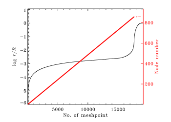
Figure 13: Properties of the mesh used for the oscillation calculation in the $1.0\,\mathrm{M}_{\odot},12\,\mathrm{R}_{\odot}$ case. The solid black line shows the logarithm of the fractional radius, against the mesh-point number (left ordinate scale). The red crosses show the nodes in the horizontal-displacement eigenfunction in a dipolar mode with frequency $20.0\,\mu{\rm Hz}$ (right ordinate scale).

In the present calculations, a mesh with 19 200 points was used. The properties of the mesh are illustrated in Fig. 13, which shows the fractional radius against the mesh-point number. It is evident that by far the majority of the points are in the core, within $3\times 10^{-3}R$, to match the g-mode-like behaviour in this region. Also shown are the locations of the nodes in the horizontal-displacement eigenfunction. In the g-mode region these are almost uniformly spaced, with approximately 20 meshpoints between adjacent nodes. The comparatively few nodes in the p-mode region have a wider spacing, the mesh satisfying also the requirement of adequately resolving the variation in the overall amplitude of the eigenfunctions.

Adiabatic oscillations satisfy a fourth-order system of equations. Boundary conditions at $r=0$ are defined by regularity conditions. At the outermost meshpoint, one boundary condition is obtained from the continuity of the perturbation to the gravitational potential and its gradient and a second from requiring that the solution transits continuously to the analytical solution of the adiabatic oscillation equations in an assumed isothermal atmosphere continuously matched to the model at the outermost point. The oscillation equations were solved using a fourth-order numerical scheme (Cash & Moore 1980). The eigenfrequencies were obtained from the condition of continuous matching of solutions integrated from the surface and the centre, at a suitable point in the core. This was achieved through a careful scan in frequency, reflecting the asymptotic distribution of frequencies, to ensure that no modes were missed. A test of the completeness was carried out on the basis of the mode orders, determined as discussed in Section A.4.

Figure 14: Absolute value of relative frequency differences, at fixed radial order, between computations with 38 400 and 19 200 points for the $1.0\,\mathrm{M}_{\odot},12\,\mathrm{R}_{\odot}$ case.

A special problem concerns discontinuities in composition and hence density, which give rise to a delta-function behaviour of $A$ (cf. Eq. 13) and, hence, in the buoyancy frequency. This occurs, for example, at the edge of the dredge-up region caused by the convective envelope, given that these models do not include diffusion and settling. A proper treatment in the model of a discontinuity would be to include it as a double point, at the same values of the continuous variables, but more typically it appears as a rapid variation in composition and density between adjacent meshpoints. A discontinuity in the model gives rise to discontinuities in the eigenfunctions, and these should ideally be dealt with by solving the equations separately on the regions separated by the discontinuities, applying jump conditions on the solution at these points. In the present calculations, each density discontinuity was replaced in the code resetting the mesh by a thin region with a very steep linear density gradient, fully resolved, and the oscillation equations were solved across this region; we ensured that the integral over the region of $A$, represented as a box function, was consistent with the jump in density. We confirmed that the relevant jump conditions on the eigenfunctions are satisfied to adequate accuracy at these points. One remaining issue is that the variation in composition is not adequately resolved in some of the models included in the comparison. In these cases, further resetting of the model (or, ideally, improvements to the evolution codes) would be desirable, and the treatment of such features in the model will also be a topic in future development and comparisons of oscillation codes.

Figure 15: Relative frequency differences at fixed radial order for $1\,\mathrm{M}_{\odot},12\,\mathrm{R}_{\odot}$, between an ASTEC model using 8509 timesteps from the ZAMS and the model used as reference with 4250 timesteps. For symbol types, see Fig. 14.

A.2 Numerical precision

Given the rapid variation in the eigenfunctions, the numerical accuracy is a concern, even given the precautions discussed above. As a test of the accuracy, we computed frequencies for all ASTEC models, doubling the number of meshpoints; the differences between the original and refined computations then give a measure of the numerical error in the former. Figure 14 shows the results in the worst case, the most evolved $1\,\mathrm{M}_{\odot}$ model. Except for g-dominated modes of degree $l=2$ at relatively low frequency, the relative errors are generally below $10^{-4}$; for the radial and p-dominated nonradial modes the errors are below $10^{-5}$, with the effects of the p-m nature being particularly visible for $l=1$. We also note that, given that the models compared are very similar, these numerical errors largely cancel in comparisons between models computed with different codes. Thus, the results obtained in the main text are unaffected by numerical errors. Even so, a comparison between different oscillation codes is obviously of interest and is planned for a future publication.

A perhaps more serious issue is the numerical accuracy of the evolution calculation resulting in the ASTEC models that have been used as reference in the present frequency comparisons. The models were computed with a fixed number of 1200 meshpoints, whose distribution changes in response to the changing structure as the models evolve. We verified that doubling the number of mesh points in the evolution calculation has a negligible effect on the results. The same is true of the number of timesteps in the model calculation, which is controlled by a parameter determining the maximum allowed change between two successive timesteps in a suitable number of model variables, throughout the stellar interior. To illustrate this, Fig. 15 shows relative frequency differences between a $1\,\mathrm{M}_{\odot}$ model requiring 8509 timesteps to reach the radius $12\,\mathrm{R}_{\odot}$ and the reference case with half as many steps.

A.3 Large frequency separation from frequency fitting

To determine $\Delta\nu_{\rm fit}$ we largely follow White et al. (2011) and carry out a weighted quadratic least-squares fit of radial-mode frequencies $\nu_{n0}$ as functions of radial order $n$ by minimising

$$\Sigma_{n}w_{n}^{2}(\nu_{n0}^{\rm(fit)}-\nu_{n0})^{2}\;,$$ (18)

where

$$\nu_{n0}^{\rm(fit)}=\nu_{0}+\Delta\nu_{\rm fit}[(n-n_{\rm max})+\alpha(n-n_{\rm max})^{2}]\;$$ (19)

(Kjeldsen et al. 2005; Mosser et al. 2013). Here $\nu_{0}$ is a reference frequency and $n_{\rm max}$ is the (generally non-integral) order corresponding to $\nu_{\rm max}$, obtained by linear interpolation of $n$ as a function of $\nu_{n0}$. Also,

$$w=\exp\left[{-(\nu_{n0}-\nu_{\rm max})^{2}\over 2\sigma^{2}}\right]\,,$$ (20)

where

$$\sigma=\gamma{\nu_{\rm max}\over 2\sqrt{2\ln 2}}\;,$$ (21)

such that the full width at half maximum of $w$ is $\gamma\nu_{\rm max}$. In the fits White et al. (2011) used $\gamma=0.25$. However, we instead followed Mosser et al. (2012) and evaluated $\gamma$ as

$$\gamma=0.66(\nu_{\rm max}/1\,\mu{\rm Hz})^{-0.12}\;,$$ (22)

based on a Gaussian approximation to the envelope of power; this value of $\gamma$ changes from around 0.25 for the Sun to 0.45 for the $(1\,\mathrm{M}_{\odot},12\,\mathrm{R}_{\odot})$ models, which have the lowest $\nu_{\rm max}$ (cf. Table 3). As an example, Fig. 16 shows the residuals from the fit for the $1\,\mathrm{M}_{\odot}$, $7\,\mathrm{R}_{\odot}$ ASTEC model.

Figure 16: Determination of $\Delta\nu_{\rm fit}$ for the solar-calibrated ASTEC $1.0\,\mathrm{M}_{\odot},7\,\mathrm{R}_{\odot}$ model. The solid line shows the residual between the radial-mode frequencies and the fitted function $\nu_{n0}^{\rm(fit)}$ (cf. Eq. 19), the diamonds indicating the location of the actual frequencies. The dashed line shows the weight function $w$ (cf. Eq. 20), using the right-hand ordinate.

Figure 17: Behaviour of $U$ (cf. Eq. 25), in three models with $M=1\,\mathrm{M}_{\odot}$, $R=7\,\mathrm{R}_{\odot}$. The dotted curve shows the original YREC model, the pluses marking the mesh points in the evolution calculation. The solid line shows the same model, after application of the correction procedure discussed in the text. For comparison, the dashed curve shows the corresponding ASTEC model, for which no correction had to be applied. The thin dot-dashed line marks $U=3$.

A.4 Dipolar-mode order

Although the analysis of the frequency comparison in Section 3.3 showed the limitations in using a formal mode order not directly related to the physical nature of the mode, a reliable formal determination of the mode order is an important feature of the frequency calculation. The order should be defined such that it is invariant for a given mode as the star evolves. This, for example, allows reliable interpolation between frequencies of modes at successive time steps in the model calculation. Also, it has been applied to ensure that all modes have been found in the frequency ranges considered. Determination of a well-defined mode order for mixed modes requires that the different characters of the eigenfunction in the g- and p-mode cavities is taken into account. For modes of degree $l\geq 2$, this can be achieved by considering the behaviour in a phase diagram defined by the vertical $\xi_{r}$ and horizontal $\xi_{\rm h}$ displacement amplitudes (Scuflaire 1974; Osaki 1975). The eigenfunction defines a curve in the $(\xi_{r},\xi_{\rm h})$ diagram, and a node in $\xi_{r}$ provides a positive (negative) contribution to the mode order if the curve crosses the $\xi_{r}=0$ axis in the counter-clockwise (clockwise) direction.

For centrally condensed stars, such as red giants, this procedure fails for dipolar modes. Following Takata (2006), we instead determined the order of such modes by means of a phase diagram based on

$${\cal Y}_{1}=(3-U){\xi_{r}\over r}+{1\over g}\left({\Phi^{\prime}\over r}-{{\rm d}\Phi^{\prime}\over{\rm d}r}\right)\;,$$ (23)

and

$${\cal Y}_{2}=(3-U){p^{\prime}\over\rho gr}+{1\over g}\left({\Phi^{\prime}\over r}-{{\rm d}\Phi^{\prime}\over{\rm d}r}\right)\;.$$ (24)

Here $r$ is distance to the centre, $g$ is the local gravitational acceleration, $\Phi^{\prime}$ is the Eulerian perturbation to the gravitational potential and $p^{\prime}$ is the Eulerian pressure perturbation. Also,

$$U={{\rm d}\ln m\over{\rm d}\ln r}={4\pi r^{3}\rho\over m}\;,$$ (25)

where $m$ is the mass internal to $r$. As shown by Takata, and in general confirmed numerically, determining the mode order based on zero crossings of ${\cal Y}_{1}$ and the direction of rotation in the phase diagram provides a unique labelling of the modes.

The properties of ${\cal Y}_{1}$ and ${\cal Y}_{2}$ near $r=0$ depend strongly on the behaviour of $3-U$. Expanding $\rho$ to ${\cal O}(r^{2})$ as

$$\rho=\rho_{\rm c}(1-\varrho_{2}r^{2}+\ldots)\;,$$ (26)

where $\rho_{\rm c}$ is the central density, we obtain

$$U=3\left(1-{2\over 5}\varrho_{2}r^{2}+\ldots\right)\;.$$ (27)

Stability requires that $\rho$ decreases with increasing $r$, and hence $\varrho_{2}>0$. Thus, $3-U$ tends smoothly to 0 for $r\rightarrow 0$ through positive values, and the factor does not affect the topology of the first terms in ${\cal Y}_{1}$ and ${\cal Y}_{2}$.

Unfortunately, some of the models involved in the frequency comparison do not satisfy this behaviour of $U$ near the centre. This is particularly serious when $U$, unphysically, exceeds 3, such that $3-U$ changes sign; this was the case for three codes. An example is shown in Fig. 17; here $U$ exceeds 3 at the innermost points of the model resulting from the evolution code, indicating an inconsistency in the way the inner boundary condition is applied. If not corrected, this behaviour causes severe problems with the determination of the order of dipolar modes. For comparison the corresponding ASTEC model is also shown; here $U$ tends smoothly to 3 as $r\rightarrow 0$. To secure a proper determination of the order, the problematic models have been corrected in a manner that provides a reasonable behaviour of $U$ near the centre. Specifically, in models where $U$ exceeds 3 in the core the outermost point $r_{U}$ where $U\geq 3$ was located. For $r\leq r_{U}$, $U$ was reset to the result of the expansion, Eq. (27), based on the expansion of $\rho$. On the interval $[r_{U},5r_{U}]$ a gradual transition was made to the original $U$, using a cubic polynomial determined such that $U$ and its first derivative are continuous. The resulting corrected $U$ is also shown in Fig. 17. This modification was applied in the code that transfers the original model to a mesh suitable for the oscillation calculations (see Section A.1). To minimise the impact on the original models, the procedure was applied only in cases where the uncorrected model was found to yield problematic dipolar mode orders. These were identified as cases where one or more adjacent computed modes did not correspond to mode orders differing by one.

The resetting of $U$ was carried out without any other readjustments of the structure, thus raising legitimate concern about the internal consistency of the resulting model. In fact, the computed frequencies for the reset and original models show relative frequency differences of less than $10^{-6}$, and in almost all cases less than $10^{-7}$, so that this has minimal consequences for the frequency comparisons carried out in the present paper. Even so, it must clearly be a goal to revise the relevant modelling codes to correct this problem at its root. In general, the treatment of the innermost points in the model causes problems in several cases, reflected in incorrect behaviour of $U$, although with no direct effect on the mode order; in these cases no resetting of the model was carried out, and the effects on the frequencies are likely insignificant, although again revisions of the modelling codes are desirable.

Appendix B Results for the RGB-calibrated models

For completeness, we include a full set of results for the RGB-calibrated models even though, as discussed in Section 3.4, they are in most cases very similar to those for the solar-calibrated models.

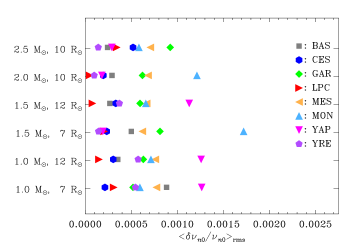
Figure 18: Root-mean-square relative differences for RGB-calibrated models in radial-mode frequencies relative to the ASTEC results, in the sense (model) - (ASTEC); the different codes are identified by the symbol shape and colour (cf. caption to Fig. 3).

Table 5: Large frequency separations $\Delta\nu_{\rm fit}$ in $\,\mu{\rm Hz}$ obtained from fits to radial-mode frequencies as functions of mode order (cf. Eq. 3 and Section A.3) for RGB-calibrated models.

$M/\,\mathrm{M}_{\odot}$	$R/\,\mathrm{R}_{\odot}$	ASTEC	BaSTI	CESAM	GARSTEC	LPCODE	MESA	MONSTAR	YAP	YREC
1.0	7.0	7.087	7.097	7.092	7.083	7.090	7.081	7.079	7.096	7.089
1.0	12.0	3.130	3.129	3.133	3.128	3.131	3.128	3.126	3.135	3.131
1.5	7.0	8.783	8.778	8.785	8.774	8.780	8.773	8.757	8.782	8.782
1.5	12.0	3.876	3.875	3.880	3.873	3.876	3.872	3.871	3.880	3.876
2.0	10.0	5.949	5.948	5.952	5.945	5.949	5.944	5.936	5.947	5.950
2.5	10.0	6.740	6.745	6.739	6.732	6.738	6.730	6.733	6.746	6.738

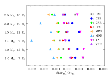
Figure 19: Relative differences for RGB-calibrated models in the large frequency separations $\Delta\nu_{\rm fit}$ obtained from fits to the radial-mode frequencies as functions of mode order (cf. Section A.3), compared with the ASTEC results, in the sense (model) – (ASTEC); the different codes are identified by the symbol shape and colour (cf. caption to Fig. 3).

Table 6: Correction factors $f_{\Delta\nu}$ (cf. Eq. 10) between the large frequency separation $\Delta\nu_{\rm fit}$ obtained from a fit to radial-mode frequencies and the value obtained from homology scaling, for RGB-calibrated models.

$M/\,\mathrm{M}_{\odot}$	$R/\,\mathrm{R}_{\odot}$	ASTEC	BaSTI	CESAM	GARSTEC	LPCODE	MESA	MONSTAR	YAP	YREC
1.0	7.0	0.9656	0.9666	0.9656	0.9651	0.9660	0.9662	0.9650	0.9677	0.9657
1.0	12.0	0.9572	0.9567	0.9575	0.9566	0.9574	0.9579	0.9564	0.9594	0.9573
1.5	7.0	0.9771	0.9763	0.9766	0.9760	0.9768	0.9774	0.9747	0.9778	0.9768
1.5	12.0	0.9677	0.9674	0.9681	0.9671	0.9678	0.9683	0.9669	0.9697	0.9676
2.0	10.0	0.9786	0.9781	0.9784	0.9779	0.9786	0.9792	0.9769	0.9792	0.9785
2.5	10.0	0.9917	0.9921	0.9909	0.9905	0.9914	0.9916	0.9911	0.9934	0.9911

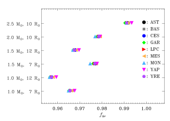
Figure 20: Correction factor $f_{\Delta\nu}$ for RGB-calibrated models in the scaling relation for the large frequency separation $\Delta\nu_{\rm fit}$ obtained from fits to the radial-mode frequencies (cf. Eq. 10). The different codes are identified by the symbol shape and colour (cf. caption to Fig. 3), with the addition of AST (for ASTEC).

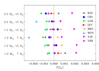
Figure 21: Differences relative to the ASTEC model in the RGB-calibrated case, in the sense (model) – (ASTEC), in the correction factors $f_{\Delta\nu}$ (cf. Eq. 10) relating the large frequency separation $\Delta\nu_{\rm fit}$ obtained from a fit to radial-mode frequencies and the value obtained from homology scaling. The different codes are identified by the symbol shape and colour (cf. caption to Fig. 3).

Table 7: Frequency $\nu_{\rm max}$, in $\,\mu{\rm Hz}$, of maximum oscillation power estimated from Eq. (8) for RGB-calibrated models.

$M/\,\mathrm{M}_{\odot}$	$R/\,\mathrm{R}_{\odot}$	ASTEC	BaSTI	CESAM	GARSTEC	LPCODE	MESA	MONSTAR	YAP	YREC
1.0	7.0	69.76	69.77	69.77	69.76	69.77	69.76	69.76	69.76	69.76
1.0	12.0	24.29	24.29	24.29	24.30	24.30	24.30	24.29	24.29	24.29
1.5	7.0	102.58	102.59	102.58	102.58	102.59	102.58	102.58	102.58	102.58
1.5	12.0	35.76	35.76	35.77	35.77	35.77	35.77	35.76	35.76	35.76
2.0	10.0	67.05	67.06	67.05	67.05	67.06	67.08	67.06	67.05	67.05
2.5	10.0	82.70	82.71	82.68	82.71	82.71	82.67	82.70	82.70	82.70

Table 8: Asymptotic dipolar g-mode period spacings $\Delta\Pi_{1}$ in s (cf. Eq. 6) for RGB-calibrated models.

$M/\,\mathrm{M}_{\odot}$	$R/\,\mathrm{R}_{\odot}$	ASTEC	BaSTI	CESAM	GARSTEC	LPCODE	MESA	MONSTAR	YAP	YREC
1.0	7.0	72.12	71.76	72.27	72.22	72.74	72.88	73.08	76.03	73.12
1.0	12.0	58.36	57.83	58.18	58.31	58.50	58.74	58.91	60.31	58.95
1.5	7.0	69.91	69.64	70.13	70.06	70.45	70.86	70.97	74.43	71.03
1.5	12.0	57.31	56.79	57.26	57.23	57.34	57.59	57.75	59.52	57.88
2.0	10.0	78.72	78.57	77.73	76.82	78.12	77.39	79.30	81.91	79.39
2.5	10.0	123.90	123.45	120.69	120.83	122.43	122.61	124.47	125.03	123.53

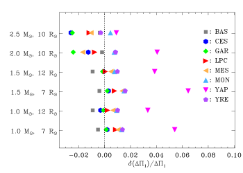
Figure 22: Relative differences for RGB-calibrated models in the asymptotic period spacing $\Delta\Pi_{1}$, compared with the ASTEC results, in the sense (model) - (ASTEC); the different codes are identified by the symbol shape and colour (cf. caption to Fig. 3).

Appendix C Properties of the asymptotic large frequency separation

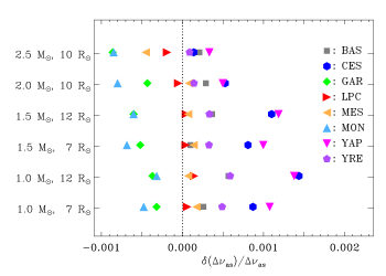
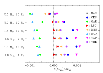
Figure 23: Relative differences in the asymptotic large frequency separation $\Delta\nu_{\rm as}$, compared with the ASTEC results, in the sense (model) - (ASTEC); the different codes are identified by the symbol shape and colour and labelled by the abbreviated name of the code (see caption to Fig. 3). The top panel shows results for solar-calibrated models and the bottom panel for the RGB-calibrated models.

Table 9: Asymptotic acoustic-mode frequency separation $\Delta\nu_{\rm as}$ (cf. Eq. 4) in $\,\mu{\rm Hz}$ for solar-calibrated models.

$M/\,\mathrm{M}_{\odot}$	$R/\,\mathrm{R}_{\odot}$	ASTEC	BaSTI	CESAM	GARSTEC	LPCODE	MESA	MONSTAR	YAP	YREC
1.0	7.0	7.792	7.794	7.799	7.790	7.793	7.794	7.789	7.801	7.796
1.0	12.0	3.507	3.509	3.512	3.505	3.507	3.507	3.506	3.512	3.509
1.5	7.0	9.504	9.505	9.512	9.500	9.504	9.505	9.497	9.513	9.507
1.5	12.0	4.263	4.264	4.267	4.260	4.263	4.263	4.260	4.268	4.264
2.0	10.0	6.432	6.434	6.435	6.430	6.432	6.433	6.427	6.435	6.433
2.5	10.0	7.227	7.229	7.228	7.221	7.226	7.224	7.221	7.229	7.228

Table 10: Asymptotic acoustic-mode frequency separation $\Delta\nu_{\rm as}$ in $\,\mu{\rm Hz}$ (cf. Eq. 4) for RGB-calibrated models.

$M/\,\mathrm{M}_{\odot}$	$R/\,\mathrm{R}_{\odot}$	ASTEC	BaSTI	CESAM	GARSTEC	LPCODE	MESA	MONSTAR	YAP	YREC
1.0	7.0	7.792	7.793	7.797	7.788	7.793	7.795	7.787	7.800	7.796
1.0	12.0	3.507	3.508	3.510	3.504	3.508	3.508	3.505	3.511	3.509
1.5	7.0	9.504	9.505	9.509	9.498	9.504	9.506	9.496	9.513	9.507
1.5	12.0	4.263	4.263	4.266	4.260	4.263	4.264	4.259	4.267	4.264
2.0	10.0	6.432	6.433	6.435	6.429	6.432	6.433	6.426	6.435	6.433
2.5	10.0	7.228	7.228	7.226	7.220	7.226	7.225	7.221	7.229	7.228

Although we argue in Section 2.1 that the asymptotic large frequency separation $\Delta\nu_{\rm as}$ does not provide an adequate accuracy for comparisons with observations (see also Mosser et al. 2013), it still represents the contribution from the bulk of the model to the frequency separation. Thus, it is of interest to compare $\Delta\nu_{\rm as}$ between the different evolution codes. Tables 9 and 10 show $\Delta\nu_{\rm as}$ for the solar-calibrated and RGB-calibrated models, computed from Eq. (4). For simplicity we replace $R_{*}$ by $R_{\rm phot}$, the photospheric radius, to avoid possible effects of differences in the models of the stellar atmospheres. The dominant variation of $\Delta\nu_{\rm as}$ with stellar properties follows the homology scaling, $\Delta\nu\propto(GM/R^{3})^{1/2}$ (see also Eq. 7) which, as discussed in Paper I, is essentially fixed. Thus, the variations between codes reflect more subtle differences in the computed structure. These variations are illustrated in Fig. 23, using the ASTEC results as reference. We note that the differences are substantially smaller than those found for $\Delta\nu_{\rm fit}$ (cf. Fig. 4). This may be caused by differences in the structure of the near-surface layers and atmospheres in the stellar models, which would affect $\Delta\nu_{\rm as}$ less than the individual frequencies. Also, these differences would have the strongest effect on high-frequency modes, and hence may affect $\Delta\nu_{\rm fit}$ more strongly than reflected in the root-mean-square frequency differences shown in Fig. 3.

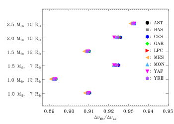
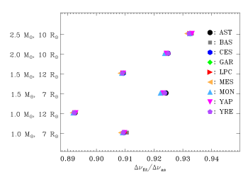
Figure 24: Ratios $\Delta\nu_{\rm fit}/\Delta\nu_{\rm as}$ between the large frequency spacing resulting from fit to the radial-mode frequencies and the asymptotic values. The symbols correspond to the different modelling codes, as defined in the caption to Fig. 3, with the addition of AST (ASTEC). The upper panel shows results for the solar-calibrated models, and the lower panel for the RGB-calibrated models.

The relation between the asymptotic value, $\Delta\nu_{\rm as}$, of the large frequency separation (see Tables 9 and 10) and $\Delta\nu_{\rm fit}$ is of some interest. Figure Fig. 24 shows their ratios. It is evident that $\Delta\nu_{\rm as}$ substantially over-estimates the actual value of $\Delta\nu$, no doubt to a large extent owing to the choice of $R_{\rm phot}$ for the upper limit in the integral in Eq. (4) rather than the location of the proper acoustic surface (see the discussion below Eq. (4), and Section 3.2). This deserves further analysis.

Appendix D Problems with the MESA atmosphere models

Figure 25: Top panel: pressure $p$ in $(1\,\mathrm{M}_{\odot},1\,\mathrm{R}_{\odot})$ models computed with MESA (solid line) and ASTEC (dashed line). Bottom panel: the pressure gradient divided by density for these models.

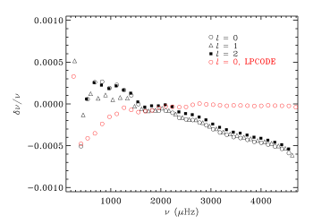
Figure 26: Relative frequency differences for the $(1\,\mathrm{M}_{\odot},1\,\mathrm{R}_{\odot})$ solar-calibrated case between MESA and ASTEC, in the sense (MESA) – (ASTEC), for $l=0$ (open circles), $l=1$ (open triangles) and $l=2$ (filled squares) in black. The differences are evaluated at fixed radial order. The red circles show corresponding results for radial modes in the LPCODE model.

In Fig. 9 we found an increase in magnitude in the frequency differences between the MESA and the ASTEC models at high frequency. This reflects what appears to be a general problem with the structure of the atmospheric models in version 6950 of MESA used in the present comparison. We illustrate this by considering the $(1\,\mathrm{M}_{\odot},1\,\mathrm{R}_{\odot})$ model in the solar-calibrated comparison track. Very similar effects are found in the other MESA cases considered.

Figure 25 compares the pressure and its derivative in the MESA and ASTEC models. The top panel shows substantial differences between the atmospheric pressures in the two models, whereas they are essentially in agreement below the photosphere. The difference between the models is even more dramatic in the bottom panel: this shows $-\rho^{-1}{\rm d}p/{\rm d}r$, which according to the equation of hydrostatic equilibrium should be equal to the gravitational acceleration $g$ and hence essentially constant in the outermost parts of the model. This is satisfied in the ASTEC model but not in the MESA model. The effect on the computed frequencies is shown in Fig. 26, compared also with the results for the corresponding LPCODE model. For the MESA model there are clearly significant differences, particularly at high frequency, as expected for model differences confined to the outermost layers; no such differences are found in the case of the LPCODE (although there are differences at low frequency, which reflect structure differences deeper in the model).

For the present comparisons these problems with the MESA models have a relatively minor effect, compared with the more substantial differences found for various other aspects of the structure. However, they would affect the comparison between observations and the MESA models, and more generally it has clearly been desirable to correct these problems with such a convenient and widely used code. We note that they have been resolved in MESA since revision 11877.

Appendix E Asteroseismic effects of thermodynamic properties

Figure 27: Relative differences in computed frequencies for the GARSTEC $1.5\,\mathrm{M}_{\odot},7\,\mathrm{R}_{\odot}$ solar-calibrated models, compared with the ASTEC results, in the sense (GARSTEC) - (ASTEC). The top panel shows results for the original GARSTEC model, and the bottom panel used the revised model, with updated treatment of the equation of state. The differences are evaluated at fixed radial order.

The original results for the GARSTEC models showed rather substantial differences, relative to the ASTEC reference, in the acoustic-mode properties. These arose from a separate treatment in the version of GARSTEC used then of the low-temperature region in the implementation of the OPAL equation of state. This has been updated in the results shown in the main part of this paper. However, since the results provide insight into the sensitivity of the frequencies to the model structure it is of interest to discuss them in some detail.

Frequency differences between the original GARSTEC and the ASTEC models for the $1.5\,\mathrm{M}_{\odot},7\,\mathrm{R}_{\odot}$ solar-calibrated case are shown in the top panel of Fig. 27. Compared with the general trends in the average radial-mode frequency differences shown in Fig. 3, there are substantial differences in the radial-mode frequencies and in the asymptotic frequency spacing and a significant discrepancy between the differences in the asymptotic and actual radial-mode frequencies. The differences in the asymptotic period spacing and consequently in the g-dominated mode frequencies are comparatively small; they are coincidentally similar to the radial-mode frequency differences.

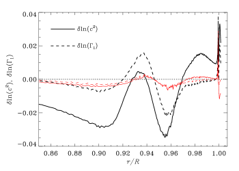
Figure 28: Logarithmic differences between the original GARSTEC and ASTEC $1.5\,\mathrm{M}_{\odot},7\,\mathrm{R}_{\odot}$ solar-calibrated models, in the sense (GARSTEC) - (ASTEC), in the outer layers of the model. The solid line shows the difference in squared sound speed $c^{2}$ and the dashed line the difference in adiabatic exponent $\Gamma_{1}$. For comparison, the thinner red lines show the corresponding differences between the revised GARSTEC and the ASTEC models.

These differences in acoustic behaviour between the original GARSTEC and ASTEC models are directly related to differences in the structure of the outer layers of the models. Figure 28 shows the logarithmic differences in squared sound speed $c^{2}=\Gamma_{1}p/\rho$ and $\Gamma_{1}$. It is evident that much of the sound-speed difference comes from the difference in $\Gamma_{1}$, in the region of helium ionisation. This is the result of significant differences between the models in the treatment of the equation of state in these regions. As shown by the red curves, these differences have been very substantially reduced by the revision of the GARSTEC models.

With the revised GARSTEC equation of state the differences in acoustic behaviour between GARSTEC and ASTEC are very small, as illustrated by the bottom panel of Fig. 27.

Appendix F Asteroseismic effects of the convective-core size

Table 11: Asymptotic dipolar g-mode period spacings $\Delta\Pi_{1}$ in s (cf. Eq. 6) for the solar-calibrated ASTEC and the original and corrected LPCODE models.

$M/\,\mathrm{M}_{\odot}$	$R/\,\mathrm{R}_{\odot}$	ASTEC	LPCODE	LPCODE
			(original)	(corrected)
2.0	10.0	78.72	73.37	78.14
2.5	10.0	123.62	117.11	122.32

Figure 29: Relative differences in computed frequencies for the LPCODE $2.5\,\mathrm{M}_{\odot},10\,\mathrm{R}_{\odot}$ solar-calibrated model, compared with the ASTEC results, ’n the sense (LPCODE) - (ASTEC). The top panel shows the original LPCODE model, while the bottom panel is for the revised model.

The original comparisons found substantial differences in g-mode frequencies between the $2.5\,\mathrm{M}_{\odot},10\,\mathrm{R}_{\odot}$ LPCODE and ASTEC models, as illustrated in the top panel of Fig. 29. Here there is excellent agreement for the radial-mode frequencies, while the g-dominated modes, and the asymptotic period spacing, show differences of around 5 %. The pattern of differences is qualitatively similar to Fig. 9, with smaller differences for the p-dominated modes. Similar effects were found in the $2.0\,\mathrm{M}_{\odot},10\,\mathrm{R}_{\odot}$ case, as illustrated by $\Delta\Pi_{1}$ in Table 11. These differences were caused by differences in the H profile in the region located between the H-burning shell and the H-discontinuity left by the first dredge-up episode (see the bottom panel in Fig. 30). Differences in the chemical profile can be traced back to a smaller receding convective core during main-sequence evolution due to an underestimation of the radiative opacities in the core. The latter was caused by the fact that the OPAL routines (Iglesias & Rogers 1993) were using the Type II set of opacity tables as soon as C and O were transformed into N by the CNO cycles. As the C and O decrement was not balanced by the N-enhancement in the opacity tables, this led to a slight underestimation of the Rosseland opacity of the core. This has now been corrected in LPCODE, as shown in Section 3 and the bottom panel of Fig. 29. However, the results provide an illustrative example of the effect on red-giant frequencies of changes to the main-sequence convective core and hence deserves a more detailed analysis. Here we focus on the solar-calibrated case; the RGB-calibrated case is very similar.

Figure 30: Top panel: variation with age in the fractional mass of the convective core, in $2.5\,\mathrm{M}_{\odot}$ solar-calibrated models. Bottom panel: resulting profiles of the hydrogen-abundance $X$ in the $10\,\mathrm{R}_{\odot}$ red-giant model. The solid and dot-dashed lines show the original and revised LPCODE models, and the dashed lines show the corresponding ASTEC model.

Relevant properties of the evolution and structure are presented in Fig. 30 (see also Paper I). The top panel shows the evolution in the fractional mass of the convective core, which defines the hydrogen profile at the end of the main sequence. It is evident that the convective core is significantly smaller, and the main-sequence phase correspondingly shorter, in the original LPCODE evolution, whereas the corrected evolution is very similar to the ASTEC case. In the $10\,\mathrm{R}_{\odot}$ model this is reflected in a slightly smaller helium-rich region in the original LPCODE model. Correcting the opacity increases the size of the convective core to close to but still slightly smaller than the ASTEC model, resulting in the much smaller frequency differences shown in the bottom panel of Fig. 29.

To investigate how the differences in structure affect the asymptotic period spacing, we express $\Pi_{0}$ (cf. Eq. 6) as

$$\Pi_{0}=2\pi^{2}{\cal I}(r_{\rm bcz})^{-1}\;,$$ (28)

where $r_{\rm bcz}$ is the radius at the base of the convective envelope, and

$${\cal I}(r)=\int_{0}^{r}N{{\rm d}r\over r}\;.$$ (29)

Also, using the equation of hydrostatic support we introduce

$$N^{2}={\cal B}{\cal G}\;,$$ (30)

separating $N^{2}$ in a dynamical and a thermodynamic part, with

$${\cal B}={g^{2}\rho\over p}\;,\qquad{\cal G}=\left({1\over\Gamma}-{1\over\Gamma_{1}}\right)\;,$$ (31)

where

$${1\over\Gamma}={{\rm d}\ln\rho\over{\rm d}\ln p}\;.$$ (32)

From Eq. (28) it follows that

$$\delta\ln\Pi_{0}\simeq-{\delta_{r}{\cal I}(r_{\rm bcz})\over{\cal I}(r_{\rm bcz})}\;,$$ (33)

neglecting the small contribution from the difference in $r_{\rm bcz}$ between the models; here, from Eqs. (29), (30) and (31),

$$\delta_{r}{\cal I}(r)\simeq{1\over 2}\int_{0}^{r}N(\delta_{r}\ln{\cal B}+\delta_{r}\ln{\cal G}){{\rm d}r\over r}\;,$$ (34)

where $\delta_{r}$ denotes the difference at fixed fractional radius. The result of the analysis is shown in Fig. 31. It is clear that Eq. (34) provides a reasonable approximation to the difference in ${\cal I}$, which is dominated by the contribution $\delta_{r}{\cal I}[\delta_{r}{\cal B}]$ from $\delta_{r}\ln{\cal B}$.

Figure 31: Differences in the partial integrals for differences in $\Pi_{0}$ (cf. Eq. 34) between the original LPCODE $2.5\,\mathrm{M}_{\odot},10\,\mathrm{R}_{\odot}$ solar-calibrated model and the ASTEC model, in the sense (LPCODE) – (ASTEC). The dashed and dash-dotted lines show the contributions $\delta_{r}{\cal I}[\delta_{r}{\cal B}]$ and $\delta_{r}{\cal I}[\delta_{r}{\cal G}]$ from $\delta_{r}{\cal B}$ and $\delta_{r}{\cal G}$, respectively, and the solid line shows their sum. For comparison, the dotted line shows the relative difference in ${\cal I}$.

To delve deeper into the origin of these differences, Fig. 32 shows the hydrogen abundance in the LPCODE and ASTEC models, as well as the logarithmic differences between the models in $p$, $\rho$, $g$ (i.e. the mass) and ${\cal B}$. The differences are predominantly in and just above the core of the model, probably related to the difference in the hydrogen profile. The change in the partial integral ${\cal I}(r)$ (cf. Fig. 31) is dominated by the core, where the LPCODE model has a higher central condensation and the larger gravitational acceleration dominates the difference in ${\cal B}$. It is interesting that the asymptotic period spacing and the mixed-mode frequencies so clearly reflect the relatively subtle difference in the hydrogen profile.

Figure 32: Top: hydrogen abundance in the ASTEC (dashed) and the original LPCODE (solid) $2.5\,\mathrm{M}_{\odot},10\,\mathrm{R}_{\odot}$ solar-calibrated models. Bottom: differences $\delta_{r}\ln p$ (dashed), $\delta_{r}\ln\rho$ (dot-dashed), $\delta_{r}\ln g$ (long dashed) and $\delta_{r}\ln{\cal B}$ (solid) between the ASTEC and the original LPCODE $2.5\,\mathrm{M}_{\odot},10\,\mathrm{R}_{\odot}$ models, in the sense (LPCODE) – (ASTEC).