Deep Robust Multilevel Semantic Cross-Modal Hashing

Abstract

Hashing based cross-modal retrieval has recently made significant progress. But straightforward embedding data from different modalities involving rich semantics into a joint Hamming space will inevitably produce false codes due to the intrinsic modality discrepancy and noises. We present a novel Robust Multilevel Semantic Hashing (RMSH) for more accurate multi-label cross-modal retrieval. It seeks to preserve fine-grained similarity among data with rich semantics,i.e., multi-label, while explicitly require distances between dissimilar points to be larger than a specific value for strong robustness. For this, we give an effective bound of this value based on the information coding-theoretic analysis, and the above goals are embodied into a margin-adaptive triplet loss. Furthermore, we introduce pseudo-codes via fusing multiple hash codes to explore seldom-seen semantics, alleviating the sparsity problem of similarity information. Experiments on three benchmarks show the validity of the derived bounds, and our method achieves state-of-the-art performance.

1 Introduction

Cross-modal retrieval, aiming to search similar instances in one modality with the query from another, has gained increasing attention due to its fundamental role in large-scale multimedia applications cao2019video ; wang2019camp ; dutta2019semantically ; zhu2019r2gan . The difficulty of the similarity measurement of data from different modals makes this task very challenging, which is known as the heterogeneity gap BaltrusaitisAM19 . An essential idea to bridge this gap is mapping different modals into a joint feature space such that they become computationally comparable, and it is widely exploited by previous work XuLYDL19 ; ZhenHWP19 ; Zhan0YZT018 . Among them, hashing-based method LiuLZWHJ18 ; ShiYZWP19 , embedding the data of interest into a low-dimensional Hamming space, has gradually become the mainstream approach due to the low memory usage and high query speed of binary codes.

Figure 1: Illustration of the robust multilevel semantic similarity-preserved codes for multi-label cross-modal data. The points filled with red color in Hamming space denote the false codes caused by the intrinsic noise of data.

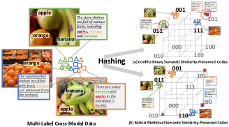While recent works have made significant progress, there are several drawbacks still in existing cross-modal hashing methods. First, embedding different modalities data sharing the same semantic into the unified hash codes is hard, since the inherent modality discrepancy and noises will inevitably cause false codes. Nevertheless, most approaches learn to hash straightforwardly with seldom considerations for this problem. They tend to embed data of different semantics into adjacency vertexes in Hamming space, which dramatically increases the collision probability of correct and false hash codes. Although some works Jiang2017Deep mentioned this problem and introduced the bit balance WangZSSS18 constraint for maximizing the information provided by each bit, it is too simple and leads to the burden of seeking proper hyper-parameter for effective learning. Second, the query always is complicated in real applications, involving rich semantics, e.g., multi-labels. But numerous work could not run such queries to return satisfying results that are consistent with the humans’ cognition on semantic similarity. They Jiang2017Deep ; HuWZP19 focus on preserving simple similarity structures (i.e., similar or dissimilar) rather than more fine-grained ones, and the used similarity information is often very sparse. We illustrate these problems in Fig. 1 (a), the image and text data associate with multiple tags, and their similarity score is not just 0 or 1. If learning hash for only keeping 0-1 similarity without proper constraints, i.e., push away the dissimilar points and pull the similar points, the conflict codes will happen, e.g.,’101’. Besides, the data of ’apple, banana’ is more similar than that of ’orange’ to the data of ’apple, orange, banana,’ but the two former’s hashing codes have the same Hamming distance with the later’s.

We observe that if the representation ability of binary codes with fixed length is adequate, hashing functions should attempt to preserve the complete fine-grained similarity structure for more accurate retrieval. Simultaneously, we can explicitly impose the distances between codes, whose similarities are zero, to be larger or equal than a specific value $\delta$ to make the learned hash codes more robust. We call $\delta$ as robust parameter and the learned codes as robust multilevel semantic similarity-preserved codes. As shown in Fig. 1(b), we hash multi-label cross-modal data into a 3-bit Hamming space according to their subtle similarity so that the distance of irrelevant data’s codes is larger or equal than 3 (i.e., the ’orange’ and ’apple, banana’ data) and the distance of the more relevant data’s codes (i.e., the ’apple, banana’ and ’orange, apple, banana’ data) is smaller than that of normal relevant data’s codes (i.e., the ’orange’ and ’orange, apple, banana’ data), then no conflict happens. Intuitively, the larger $\delta$ is, the more robust learned codes are, and the more levels of the semantic similarity can be encoded. We could embody this constraint in the objective of hashing learning. However, endowing too large $\delta$ is not practical due to the limited coding power of length-fixed binary codes and the uncertainty of the hashing process. The question thus becomes how to find an appropriate $\delta$. In theory, as the Hamming space and the semantic similarity information are definite, the assumption that all data are well hashing, i.e., no false codes, can be helpful to reduce uncertainty and ease the derivation of the range of effective $\delta$.

Here, we briefly describe our answer to the above question under the previous assumption. We would like to encode semantic and similarity information of data to $K$-bit binary codes. The maximum number of $K$-bit codes with minimum pairwise Hamming distance $\delta$ is certain. According to the information coding theory, the log of this number should be larger than the amount of semantic information, and the $\delta$-bits should be able to encode the neighbor similarity information of each point. Based on these facts, we derive the bounds of proper $\delta$ and detail the process in Sec. 3.2.

Inspired by the above observation, we propose a novel deep Robust Multilevel Semantic Hashing (RMSH), which treats preserving the complete multilevel semantic similarity structure of multi-label cross-modal data with theoretically guaranteed distance constraint between dissimilar data, as the objective to learn hash functions. For this, a margin-adaptive triplet loss is adopted to control the distance of dissimilar points in Hamming space explicitly, meanwhile embedding similar points with a fine-grained level. To alleviate the sparsity problem of similarity information, we further present fusing multiple hash codes at the semantic level to generate pseudo-codes, exploring the seldom-seen semantics. The main contributions are summarized as follows.

• A novel hashing method, named RMSH, is proposed to learn multilevel semantic similarity-preserved codes for accurate multi-label cross-modal retrieval. In which, to exploit the finite Hamming space for improving the robustness of learned codes, we require the distance between codes of dissimilar points satisfies larger than a specific value. For more effective learning, we perform a theoretical analysis of this value and bring out its effective range.

• To capture the fine-grained semantic similarity structure in coupling with the elaborated distance constraint, we present a margin-adaptive triplet loss. Moreover, a new pseudo-codes network is introduced, tailored to explore more rare and complicated similarity structures.

• Extensive experimental results demonstrate the effectiveness of the derived bounds, and the proposed RMSH approach yields the state-of-the-art retrieval performance on three cross-modality datasets.

2 Related work

In this section, we briefly review related works concerning cross-modal hashing methods.

The cross-modal hashing cao2018cross ; zhang2018attention ; chen2019two ; lu2019flexible ; li2019coupled ; su2019deep can be grouped into two types, unsupervised and supervised. The former utilizes the co-occurrence information of the multi-modal pair (e.g., image-text) to maximize their correlation in the common Hamming space. The representative is Collective Matrix Factorization Hashing (CMFH) Ding2014Collective , which generates unified hash codes for multiple modalities by performing collective matrix factorization from different views. The supervised ones aim to preserve semantic similarity. Semantic Correlation Maximization (SCM) Zhang2014Large uses hash codes to reconstruct semantic similarity matrix. Semantics-Preserving Hashing (SePH) Lin2015Semantics minimizes KL-divergence between the hash codes and semantics distributions. Recently, the success of deep learning prompted the development of cross-modal hashing. Cross-Modal Deep Variational Hashing (CMDVH) LiongLT017 infers fusion binary codes from multi-modal data as the latent variable for model-specific networks to approximate. Self-supervised Adversarial Hashing (SSAH) LiDL0GT18 incorporates the adversarial learning into cross-modal hashing. Equally-Guided Discriminative Hashing (EGDH) ShiYZWP19 jointly considers semantic structure and discriminability to learn hash functions. Similar to CMDVH, but Separated Variational Hashing Networks (SVHNs) HuWZP19 learns binary codes of semantic labels as the latent variable. Despite their effectiveness, most of them ignore the exploitation of limited representative of binary codes for reducing the impact of the modality gap, and they fail to preserve fine similarity for more accurate multi-label cross-modal retrieval.

Figure 2: The architecture of the proposed RMSH includes two modality-specific hashing networks and a pseudo-codes network (PCN). The RMSH first takes multi-modal triplets into hashing networks to obtain hash codes, which are then manipulated by PCN to generated codes with seldom-seen semantics. Finally, a margin-adaptive triplet loss equipped with the pre-computed robust parameter $\delta$ is coupled with the weighted classification loss and quantization loss to learn robust multilevel semantic similarity-preserved codes.

3 The proposed approach

In this section, we first give the problem definition and the effective bounds of the robust parameter defined in Sec. 1. Then, the configurations of the proposed RMSH are detailed, including two hashing networks, a pseudo-code network, and the corresponding objective function. An overview of the RMSH is illustrated in Fig. 2.

3.1 The Problem Definition

Without loss of generality, we use bi-modality (e.g., image and text) retrieval for illustration in this paper. Assume that we are given a multi-modal dataset $\mathbf{D}=\{\mathbf{X}$, $\mathbf{Y}$, $\mathbf{L}\}$, where $\mathbf{X}=\{x_{i}\}_{i=1}^{N}$, $\mathbf{Y}=\{y_{i}\}_{i=1}^{N}$, $\mathbf{L}=\{l_{i}\}_{i=1}^{N}$ denotes the image modality, text modality, and corresponding semantic labels, respectively. $x_{i}$ can be features or raw pixels of images, $y_{i}$ is textual description or tags, semantic label $l_{i}\in\{0,1\}^{C}$, where C is the number of class. For any two samples, we define the cross-modal similarity $\mathbf{S}$ as $S_{ij}=\frac{|l_{i}\cap l_{j}|}{max\{|l_{i}|,|l_{j}|\}}$. Given training data $\mathbf{X}$, $\mathbf{Y}$ and $\mathbf{S}$, our goal is to learn two hash functions: $h^{(x)}(x)=b^{(x)}\in\{-1,1\}^{K}$ for the image modality and $h^{(y)}(y)=b^{(y)}\in\{-1,1\}^{K}$ for the text modality, where $K$ is the length of the binary code, such that the similarity relationship $\mathbf{S}$ is preserved and distances between dissimilar data are larger or equal than a positive integer $\delta$ $(<K)$ for robustness, i.e., $\forall$ $x_{i}\in\mathbf{X}$, $y_{j}$, $y_{k}\in\mathbf{Y}$, if $S_{ij}\geq S_{ik}$, then the Hamming distance of their binary codes should satisfy $d_{H}(b_{i}^{(x)},b_{j}^{(y)})$ $\leq$ $d_{H}(b_{i}^{(x)},b_{k}^{(y)})$, and vice versa, if $S_{ij}=0$, then $d_{H}(b_{i}^{(x)},b_{j}^{(y)})$ $\geq$ $\delta$, $\delta$ is named as robust parameter. Intuitively, a larger $\delta$ makes codes more robust, but it cannot be too large due to the finite representation power of $K$-bit binary codes. In what follows, we investigate how to properly set this parameter to obtain the balance between robustness and compactness.

3.2 Bounds of Effective Robust Parameter

To learn robust hashing codes effectively, we give the range of effective robust parameter $\delta$ in this section. In essential, the goal of deep supervised hashing is encoding semantic information $H(\boldsymbol{L})$ and similarity information $H(\boldsymbol{S_{*,:}})$ of data by $K$-bit binary codes, where $H$ denotes entropy function. Therefore, according to the coding theory guruswami2012essential , we have the following two facts. (1) To make sure that different semantics have unique codes and the distances between the codes of irrelevant samples are larger or equal than $\delta$, the number of $K$-bit binary codes that satisfy pairwise minimum distance $\delta$ should be larger than $2^{H(\boldsymbol{L})}$. (2) $\delta$ bits should be able to encode the neighborhood semantic similarity information $H(\boldsymbol{S_{*,:}})$ of each sample $*$. Based on these two facts, we derive the bounds of effective $\delta$ as follows. For simplicity’s sake, we assume that all data sharing the same semantic are embedded into the same codes to eliminate the influence of noise.

1) Upper bound. By the fact (1), we have:

$$2^{H(\boldsymbol{L})}\leq A(K,\delta)$$ (1)

where $A(K,\delta)$ denotes the maximum number of K-bit binary codes with pairwise minimum Hamming distance $\delta$, i.e., $A(K,\delta)=|\{b|b\in\{-1,1\}^{K},for\ \forall\ b_{i}\neq b_{j},d_{H}(b_{i},b_{j})\geq\delta\}|$. To obtain the range of effective $\delta$, we need estimate $A(K,\delta)$. However, an accurate estimation of $A(K,\delta)$ is challenging, which is still unsolved. Alternatively, its bounds are well studied HelgertS73 ; AgrellVZ01 ; BelliniGS14 . Towards our goal, we introduce a well-known lower-bound of $A(K,\delta)$ to derive the upper-bound of $\delta$.

Lemma 1.

(Gilbert-Varshamov Bound gilbert1952comparison ). Given $\delta$, $K\in\mathbb{N}$ be such that $\delta\leq K$, we have:

$$\frac{2^{K}}{\sum_{i=0}^{\delta-1}\binom{K}{i}}\leq A(K,\delta)$$ (2)

To proof the Lemma 1, we first give the definition of Hamming Ball and then give the proof.

Definition 1.

(Hamming Ball). Let $\delta$, $K\in\mathbb{N}$ such that $\delta\leq K$. For $\forall$ $x$ $\in\Omega=\{-1,1\}^{K}$, the ball $B_{\delta}^{K}(x)$ denotes the set of vectors with distance from the $x$ less than or equal to $\delta$ and is defined as $B_{\delta}^{K}(x)=\{y\in\Omega|d_{H}(y,x)\leq\delta\}$. Its volume is defined as $|B_{\delta}^{K}(x)|=\sum_{i=0}^{\delta}\binom{K}{i}$, and $|B_{\delta}^{K}|$ for short.

Proof.

Let $\Omega^{(\delta)}$ denotes the greatest subset of $\Omega=\{-1,1\}^{K}$ that $\forall$ $c,c^{\prime}$ $\in$ $\Omega^{(\delta)}$, $d_{H}(c,c^{\prime})\geq$ $\delta$ and $A(K,\delta)=|\Omega^{(\delta)}|$, $\varepsilon=\delta-1$. For $\forall$ $y\in$ $\Omega$, there exists at least one $c\in$ $\Omega^{(\delta)}$ such that $d_{H}(y,c)\leq\varepsilon$, otherwise y$\in$ $\Omega^{(\delta)}$. Hence, $\Omega$ is contained in the union of all balls $B_{\varepsilon}^{K}(c)$, $c\in$ $\Omega^{(\delta)}$, that is $\Omega\subseteq\bigcup_{c\in\Omega^{(\delta)}}B_{\varepsilon}^{K}(c)$, then we have $|\Omega|\leq\sum_{c\in\Omega^{(\delta)}}|B_{\varepsilon}^{K}(c)|=|\Omega^{(\delta)}|\cdot|B_{\varepsilon}^{K}(c)|$, thus $A(K,\delta)=|\Omega^{(\delta)}|\geq\frac{|\Omega|}{|B_{\varepsilon}^{K}(c)|}=\frac{2^{K}}{\sum_{i=0}^{\delta-1}\binom{K}{i}}$. ∎

As we see that if $2^{H(\boldsymbol{L})}$ is smaller than the lower-bound of $A(K,\delta)$, Eq. (1) also holds. By the Lemma 1, we thus have:

$$2^{H(\boldsymbol{L})}\leq\frac{2^{K}}{\sum_{i=0}^{\delta-1}\binom{K}{i}}$$ (3)

Still, the computation of $\sum_{i=0}^{\delta-1}\binom{K}{i}$ in Eq. (3) is hard. Here, we show an upper-bound of this value via the entropy bound of the volume of a Hamming ball.

Lemma 2.

(Volume of Hamming ball). Given $\delta$, $K\in\mathbb{N}$ and $\delta=pK$, $p\in$ $[0,1/2]$, we have:

$$|B^{K}_{\delta}|\leq 2^{H(p)K}$$ (4)

where $H(p)$ $=-p\log p-(1-p)\log(1-p)$.

Proof.

$$\frac{|B^{K}_{\delta}|}{2^{H(p)K}} =\frac{\sum_{i=0}^{\delta}\binom{K}{i}}{p^{-pK}(1-p)^{-(1-p)K}}$$

$$=\sum_{i=0}^{pK}\binom{K}{i}(1-p)^{K}(\frac{p}{1-p})^{pK}$$

$$<\sum_{i=0}^{pK}\binom{K}{i}(1-p)^{K}(\frac{p}{1-p})^{i}(\mathrm{since}\ \frac{p}{1-p}<1,i\leq pK)$$

$$=\sum_{i=0}^{pK}\binom{K}{i}(1-p)^{K-i}p^{i}=1(\mathrm{binomial}\ \mathrm{theorem})$$

∎

By the Lemma 2 and Eq. (3), we can obtain a computable lower-bound of $A(K,\delta)$. By this bound, we give the theorem about the upper bound of effective $\delta$ in our problem.

Theorem 1.

For information $H(\boldsymbol{L})$, if using $K$-bit binary codes to encode $l\in\boldsymbol{L}$ such that for $\forall$ $l_{i}\neq l_{j}$, $d_{H}(b_{i},b_{j})\geq\delta$, $\delta\leq K/2$, then, $\delta$ should satisfy:

$$H\big{(}\frac{\delta-1}{K}\big{)}\leq 1-\frac{H(\mathbf{\boldsymbol{L}})}{K}$$ (5)

Proof.

By the the Lemma 2 and to make Eq. (3) always hold, we have:

$$2^{H(\mathbf{\boldsymbol{L}})}\leq\frac{2^{K}}{2^{H(\frac{\delta-1}{K})K}}\leq\frac{2^{K}}{\sum_{i=0}^{\delta-1}\binom{K}{i}}\leq A(K,\delta)$$

whence $H(\frac{\delta-1}{K})\leq 1-\frac{H(\boldsymbol{L})}{K}$. ∎

In experiments, we can estimate $H(\boldsymbol{L})$$=H(\boldsymbol{L}_{1},$$\boldsymbol{L}_{2},$$\dots,$$\boldsymbol{L}_{C})$ $=$ $\sum_{i=1}^{C}H(\boldsymbol{L}_{i})$ by assuming independence between tags for simplicity and each tag $\boldsymbol{L}_{i}$ follows a Bernoulli distribution, i.e., $\boldsymbol{L}_{i}\sim B(\theta_{i})$. The estimation of $\theta_{i}$ can be $\hat{\theta_{i}}=\frac{1}{N}\sum_{n=1}^{N}\mathbb{I}(l_{n,i}=1)$, $l\in\mathbf{L}$, where $\mathbb{I}\{*\}$ is indicator function. Then, given code length $K$ and $\delta$, we can investigate whether the value of $\delta$ is larger than the effective range. In our experiments, we found that the upper-bound of the effective $\delta$ is always less than $K/2$, which is preferred set by previous works.

2) Lower bound. Let $H_{*}$ denote $H(\boldsymbol{S_{*,:}})$, by the fact (2) we have $\delta\geq\mathop{\max}_{*=1:N}\{H_{*}\}$. However, as $S$ is sparse, we could relax $\delta\geq\mathop{\max}_{*=1:N}\{H_{*}\}$ by making the $\delta$ be larger than most $H_{*}$ to ensure $\delta$ bits can encode the semantic neighbors of each sample with a certain probability. By Chebyshev’s Inequality, we have:

$$P\{H_{*}\leq\delta\}\geq 1-\frac{D(H_{*})}{(\delta-E(H_{*}))^{2}}$$ (6)

where $E(H_{*})=\frac{1}{N}\sum_{i=1}^{N}H_{i}$, $D(H_{*})=\frac{1}{N}\sum_{i=1}^{N}(H_{i}-E(H_{*}))^{2}$. If $P\{H_{*}\leq\delta\}=p$, $1>p>1/2$, we have:

$$\delta\geq\sqrt{\frac{D(H_{*})}{1-p}}+E(H_{*})$$ (7)

We estimate $H_{i}=-\sum_{j=1}^{|l_{i}|}p(s_{i}=\frac{j}{|l_{i}|})\log p(s_{i}=\frac{j}{|l_{i}|})\leq|l_{i}|$, $p(s_{i}=\frac{j}{|l_{i}|})=\frac{\sum_{*}\mathbb{I}(S_{i,*}=j/|l_{i}|)}{\sum_{*}\mathbb{I}(|l_{i}\cap l_{*}|=S_{i,*}\cdot|l_{i}|)}$, $s_{i}\in S_{i,:}$. For simple computation, we substitute $H_{i}$ with $|l_{i}|$ in experiments.

Combing Eqs. (5) and (7), we obtain the final bounds of effective robust parameter $\delta$. In practice, we can pre-determine the range of high quality $\delta$ by substituting the corresponding value into Eq. (5) and (7) when given training set information and avoid the burden of seeking proper value for effective learning. It is worth note that the performance of different $\delta$ within bounds is not significantly different, setting any value in bounds is OK in practice. Furthermore, if we want to find optimal $\delta$, our theoretical results can guarantee the performances within bound are better than those without bound, which significantly reduces the search range of optimal hyper-parameter. Therefore, setting the special value within the bound is not difficult. The experimental results in Sec. 4.4 demonstrate the effectiveness of the derived bounds.

3.3 Network Architecture

The architecture of RMSH is illustrated in Fig. 2, which seamlessly integrates three parts: the image hashing, the text hashing, and the pseudo-codes networks.

Deep Hashing Networks. We build image and text hashing as two deep neural networks via adding two fully-connected layers with tanh function on the top feature layer of commonly-used modality-specific deep models, e.g., CNN model ResNet for image modality, BOW or sentence2vector for text modality. These two layers as the hash functions transform the feature $x_{i}$, $y_{i}$ into binary-like codes $z_{i}^{(x)}$, $z_{i}^{(y)}$$\in$$\mathbb{R}^{K}$. Then, we obtain the hash codes of modality $*$ by $b_{i}^{(*)}=sgn(z_{i}^{(*)})$, where $sgn(z)$ is the sign function.

Pseudo-codes Network (PCN). The input data are always imbalanced due to the sparsity problem of multi-labels, which results in the difficulty of capturing complicated similarity structure across modality. To handle this problem, inspired by work AlfassyKASHFGB19 , we propose pseudo-codes networks to manipulate the binary-like codes at the semantic level for generating codes of rare semantics, which are mixed with original codes to explore complicated similarity structure. We defined two types of code operations, i.e., union and intersection, as two fully-connected networks:

$$z_{1\oplus 2} =f_{u}(z_{1},z_{2})\equiv tanh(W_{u}[z_{1},z_{2}])$$ (8)

$$z_{1\otimes 2} =f_{t}(z_{1},z_{2})\equiv tanh(W_{t}[z_{1},z_{2}])$$

where $[\cdot,\cdot]$ denotes the concatenation operation. $W_{u},W_{t}$ $\in\mathbb{R}^{K\times 2K}$ are weights to be learnt. $z_{1\oplus 2}=f_{u}(z_{1},z_{2})$ with label $l_{u}=l_{1}\oplus l_{2}=l_{1}\cup l_{2}$. $z_{1\otimes 2}=f_{t}(z_{1},z_{2})$ with label $l_{t}=l_{1}\otimes l_{2}$, defined as $l_{1}\cap l_{2}$.

3.4 Objective Function

To preserve multilevel semantic similarity and fully exploit the space between dissimilar points in Hamming space, we formulate the goal in Sec 3.1 as follows: for $\forall$ $b_{i}$, $b_{j}$, $b_{k}$, 1) if $S_{i,j}$$>$$S_{i,k}$$>0$, then $d_{H}(b_{i},b_{k})$$-$$d_{H}(b_{i},b_{j})$$\geq$$(S_{i,j}$$-$$S_{i,k})$$\cdot\delta$. 2) if $S_{i,j}$$=$$0$, then $d_{H}(b_{i},b_{j})$$\geq$$\delta$. The first goal is to preserve the ranking information of similar points by an adaptive margin. The second goal is to keep the minimum distance between dissimilar points. We couple these two goals in a scheme of margin-adaptive triplets, that is:

$$\mathcal{L}_{t}(b_{i},b_{j},b_{k}) =y_{i,j}\cdot y_{i,k}\cdot[d_{H}(b_{i},b_{j})-d_{H}(b_{i},b_{k})+\alpha]_{+}$$ (9)

$$+(1-y_{i,j})[\delta-d_{H}(b_{i},b_{j})]_{+}+(1-y_{i,k})[\delta-d_{H}(b_{i},b_{k})]_{+}$$

where $[\cdot]_{+}=max\{0,\cdot\}$, $y_{i,j}=\mathbb{I}(S_{i,j}>0)$, $y_{i,k}=\mathbb{I}(S_{i,k}>0)$, $\mathbb{I}$ is indication function, $\alpha=\delta(S_{i,j}-S_{i,k})$, is adaptive to the discrepancy of similarity level and $\delta$ controls the distance of dissimilar points. Given a triplet of multi-modal data $x_{\{1,2,3\}}$, $y_{\{1,2,3\}}$ and their labels $l_{\{1,2,3\}}$, we can obtain five hash codes for each modality, i.e., $b_{\{1,2,3\}}$, and $b_{4}=sgn(f_{u}(z_{1},z_{2}))$, $b_{5}=sgn(f_{t}(z_{1},z_{2}))$. Note that in principle we can generate more pseudo-codes using the PCN network but for simplicity and w.l.o.g., here only a set involving two codes are used. We partition them into the intra-modality triplets $b_{\{1,2,3\}}$, $b_{\{1,2,4\}}$, $b_{\{1,2,5\}}$, and the inter-modality triplets $\{b_{1}^{(y)},b_{\{2,3\}}^{(x)}\}$, $\{b_{2}^{(y)},b_{\{1,3\}}^{(x)}\}$, $\{b_{3}^{(y)},b_{\{1,2\}}^{(x)}\}$, each of which reflects some aspect of the similarity structure and corresponds to a separate loss term in the final loss.

To mine the effective information in each triplets quickly, we select one point $b_{*}$ from each triplet with most tags as the reference point and re-order other points as $\{b_{*},b_{*,1},b_{*,2}\}$, where $b_{*,1}$ is the one that is more similar to $b_{*}$ than the other $b_{*,2}$. Then, we substitute them into Eq. (9) and obtain the used triplet loss as $\mathcal{L}_{t}(b_{\{1,2,3\}})=\mathcal{L}_{t}(b_{*},b_{*,1},b_{*,2})$, where $\alpha=\frac{|l_{*}\cap l_{*,1}|-|l_{*}\cap l_{*,2}|}{|l_{*}|}\cdot\delta$.

The final triplet loss for one modality is defined as:

$$\mathcal{L}_{tr}( b_{\{1,2,3\}}^{(x)})=\lambda_{1}(\sum_{i=3}^{5}\mathcal{L}_{t}(b^{(x)}_{\{1,2,i\}}))+\lambda_{2}(\mathcal{L}_{t}(b_{1}^{(y)},b_{\{2,3\}}^{(x)})$$ (10)

$$+\mathcal{L}_{t}(b_{2}^{(y)},b_{\{1,3\}}^{(x)})+\mathcal{L}_{t}(b_{3}^{(y)},b_{\{1,2\}}^{(x)}))$$

where $\lambda_{1}$, $\lambda_{2}$ control the weight of intra-modal and inter-modal similarity loss, respectively.

Besides, we adopt weighted cross-entropy loss to ensure that each individual hashing codes consistent with its own semantics, especially for the pseudo-codes from fusion, and the loss is defined as follows:

$$\mathcal{L}_{cl}(b)=-\sum_{j=1}^{C}\big{(}w_{p}\cdot l_{j}\log(\hat{l_{j}})+(1-l_{j})\log(1-\hat{l_{j}})\big{)}$$ (11)

where $\hat{l}$ is the predicted value of RMSH, and $w_{p}$ is the weight of positive samples.

Finally, the overall objective for N training triplets $\{b_{i1},$ $b_{i2},$$b_{i3}\}_{i=1}^{N}$ of RMSH is defined as follows:

$$\mathop{min}_{\theta}\mathcal{L} =\sum_{i=1}^{N}\big{(}\sum_{j=1}^{3}\mathcal{L}_{cl}(b^{(x,y)}_{ij})+\mathcal{L}_{tr}(b^{(x,y)}_{i\{1,2,3\}})$$ (12)

$$+\lambda_{3}(\mathcal{L}_{cl}(b^{(x,y)}_{i4})+\mathcal{L}_{cl}(b^{(x,y)}_{i5}))\big{)}$$

$$s.t.\ b^{(x)},b^{(y)}\in\{-1,1\}^{K}$$

where $\lambda_{3}$ balances the classification loss of pseudo-codes, $\theta$ is the parameter of image hashing, text hashing, and PCN.

3.5 Optimization

Since the Eq. (12) is a discrete optimization problem, we follow the work Wu2017Deep to solve this problem. We relax $b$ as $z$ by introducing quantization error $||z-b||_{2}^{2}$, and substitute Hamming distance with Euclidean distance, i.e. $d(z_{1},z_{2})=||z_{1}-z_{2}||_{2}^{2}$. The Eq. (12) is rewritten as follows:

$$\mathop{min}_{\theta,b}\mathcal{L} =\sum_{i=1}^{N}\big{(}\sum_{j=1}^{3}L_{cl}(z^{(x,y)}_{ij})+\lambda_{3}(\sum_{j=4}^{5}L_{cl}(z^{(x,y)}_{ij}))$$ (13)

$$+L_{tr}(z^{(x,y)}_{i\{1,2,3\}})+\lambda_{4}\sum_{j=1}^{3}||z^{(x,y)}_{ij}-b_{ij}||_{2}^{2}\big{)}$$

$$s.t.\ b\in\{-1,1\}^{K}$$

where $z^{(*)}_{i4}=f_{u}(z^{(*)}_{i1},z^{(*)}_{i2})$, $z^{(*)}_{i5}=f_{t}(z^{(*)}_{i1},z^{(*)}_{i2})$. $\lambda_{4}$ controls the weight of quantization error. In the training phase, we let $b_{i}$ $=b_{i}^{(x)}$ $=b_{i}^{(y)}$ for better performance. We adopt an alternating optimization strategy to learn $\theta$ and $b$ as follows.

1) Learn $\theta$ with $b$ fixed. When $b$ is fixed, the optimization for $\theta$ is performed using stochastic gradient descent based on Adaptive Moment Estimation (Adam).

2) Learn $b$ with $\theta$ fixed. When $\theta$ is fixed, the problem in Eq. (13) can be reformulated as follows:

$$\mathop{max}_{b} \lambda_{4}\sum_{i=1}^{N}\big{(}b_{i}^{T}(z^{(x)}_{i}+z^{(y)}_{i})\big{)}$$ (14)

$$s.t.\ b\in\{-1,1\}^{K}$$

We can find that the binary code $b_{i}$ should keep the same sign as $z^{(x)}_{i}+z^{(y)}_{i}$, i.e., $b_{i}=sgn(z^{(x)}_{i}+z^{(y)}_{i})$.

4 Experiments and Discussions

4.1 Datasets

Microsoft COCO Lin2014Microsoft contains 82,783 training and 40,504 testing images. Each image is associated with five sentences (only the first sentence is used in our experiments), belonging to 80 most frequent categories. We use all training set for training and sample 4,956 pairs from the testing set as queries.

MIRFLICKR25K HuiskesL08mir contains 25,000 image-text pairs. Each point associates with some of 24 labels. We remove pairs without textual tags or labels and subsequently get 18,006 pairs as the training set and 2,000 pairs as the testing set. The 1386-dimensional bag-of-words vector gives the text description.

NUS-WIDE civr09nuswide contains 260,648 web images, belonging to 81 concepts. After pruning the data without any label or tag information, only the top 10 most frequent labels and the corresponding 186,577 text-image pairs are kept. 80,000 pairs and 2,000 pairs are sampled as the training and testing sets, respectively. The 1000-dimensional bag-of-words vector gives the text description. We sampled 5,000 pairs of the training set for training.

Table 1: Comparison (NDCG@500) of different cross-modal hashing methods on three datasets with different code length. The best result is shown in boldface.

Task	Method	MIRFLICKR25K				NUS-WIDE				MS COCO
		16bits	32bits	64bits	128bits	16bits	32bits	64bits	128bits	16bits	32bits	64bits	128bits
I $\to$ T	CMFH	0.2926	0.3154	0.3193	0.3282	0.4875	0.5012	0.5270	0.5394	0.2224	0.2571	0.2899	0.3098
	UCH	0.3017	0.3114	0.3197	0.3362	0.5202	0.5175	0.5227	0.5175	0.2239	0.2588	0.2757	0.3143
	SePH	0.3310	0.3522	0.3667	0.3811	0.5726	0.5809	0.5867	0.6043	0.2266	0.2681	0.3113	0.3375
	DCMH	0.3857	0.4013	0.4162	0.4046	0.5942	0.6239	0.6353	0.6392	0.2257	0.2661	0.3089	0.3147
	TDH	0.4379	0.4491	0.4491	0.4458	0.6196	0.6242	0.6305	0.6324	0.2447	0.2692	0.2946	0.3138
	SSAH	0.4203	0.4392	0.4626	0.4753	0.6026	0.6331	0.6263	0.6144	0.1955	0.2797	0.3157	0.3917
	SVHN	0.4186	0.4354	0.4675	0.4895	0.6039	0.6324	0.6486	0.6501	0.2526	0.2930	0.3270	0.3811
	RMSH	0.4592	0.4940	0.5180	0.5183	0.6148	0.6401	0.6497	0.6574	0.3037	0.3724	0.3855	0.3998
T $\to$ I	CMFH	0.2857	0.3079	0.3115	0.3138	0.4642	0.4775	0.4998	0.5091	0.1982	0.2182	0.2398	0.2539
	UCH	0.3027	0.3000	0.3157	0.3051	0.4923	0.5103	0.5008	0.5232	0.1895	0.2356	0.2569	0.2687
	SePH	0.3085	0.3245	0.3168	0.3582	0.5264	0.5285	0.5245	0.5337	0.1968	0.2367	0.2627	0.2839
	DCMH	0.3719	0.3819	0.3877	0.3894	0.5375	0.5451	0.5438	0.5463	0.1885	0.2122	0.2544	0.2601
	TDH	0.3789	0.4084	0.3924	0.3937	0.5329	0.5340	0.5368	0.5306	0.2249	0.2420	0.2521	0.2712
	SSAH	0.3648	0.3815	0.3710	0.3707	0.5262	0.5428	0.5583	0.5375	0.1870	0.2382	0.2469	0.3114
	SVHN	0.3985	0.4434	0.4483	0.4604	0.5486	0.5702	0.5831	0.5885	0.2313	0.2664	0.2780	0.3163
	RMSH	0.4379	0.4533	0.4562	0.4628	0.5744	0.5921	0.5900	0.5999	0.2897	0.3080	0.3050	0.3175

4.2 Evaluation protocol and Baselines

Evaluation protocol. We perform cross-modal retrieval with two tasks. (1) Image to Text (I $\to$ T): retrieve relevant data in the text training set using a query in the image test set. (2) Text to Image (T $\to$ I): retrieve relevant data in the image training set using a query in the text test set. Particularly, to evaluate the retrieval performance of multi-label data, we adopt the Normalized Discounted Cumulative Gain (NDCG) Kalervo2000IR as the performance metric, which is defined as follows, since the NDCG can evaluate the ranking by penalizing errors according to the relevant score and position.

$$NDCG@p=\frac{1}{Z}\sum_{i=1}^{p}\frac{2^{r_{i}}-1}{\log(1+i)}$$ (15)

where Z is the ideal $DCG@p$ and calculated form the correct ranking list, and $p$ is the length of list. $r(i)=|l_{q}\cap l_{i}|$ denotes the similarity between the $i$-th point and the query, following the definition in work zhao2015deep . $l_{q}$ and $l_{i}$ denote the label of the query and $i$-th position point.

Besides, the commonly-used precision-recall curve is used as a metric to evaluate the performance, where we consider two points are relevant if they share at least one tag.

Baselines. We compare our proposed RMSH with six cross-modal hashing methods CMFH Ding2014Collective , UCH li2019coupled , SePH Lin2015Semantics , DCMH Jiang2017Deep , TDH DengCLGT18 , SSAH LiDL0GT18 , SVHN HuWZP19 . For a fair comparison, all shallow methods take the deep off-the-shelf features extracted from ResNet-152 He2015Deep pre-trained on ImageNet as inputs, and all deep models are implemented carefully with the same CNN sub-structures for image data and the same multiple fully-connect layers for textual data. The hyper-parameters of all baselines are set according to the original papers or experimental validations.

4.3 Implementation details.

Our RMSH method is implemented with Tensorflow. We use ResNet He2015Deep pre-trained on ImageNet as the CNN model in image hashing to extract features of image modality. For the MS COCO dataset, the 4800-dimensional Skip-thought vector KirosZSZUTF15 gives the sentence description. The structure of two hashing layers is $D^{(*)}\to 1024\to K$-bit length, where $D$ is the dimension of * modality’s feature. For fast training, we only optimize the hashing layers with the pre-trained CNN sub-structures (no fine-tuned on the target dataset for a fair comparison with other shallow methods) fixed for all deep methods. In all experiments, we set the batch size to 128, epochs to 50, $\lambda_{1}$, $\lambda_{2}$, $\lambda_{3}$, and $\lambda_{4}$ to 0.01, 0.1, 0.1, 0.1, learning rate to 0.001, $\delta$ by the derived results in Sec. 3.2, $w_{p}$ to 20 for NUS-WIDE and MIRFLICKR25K datasets, 30 for MS COCO dataset.

@MIRFLICKR25K (I$\to$T)	@NUS-WIDE (I$\to$T)	@MS COCO (I$\to$T)
@MIRFLICKR25K (T$\to$I)	@NUS-WIDE (T$\to$I)	@MS COCO (T$\to$I)

Figure 3: Precision-Recall curves on MIRFLICKR25K, NUS-WIDE, and MS COCO datasets.

Figure 4: Retrieval examples of ’Text to Image’. Red border denotes irrelevant; blue denotes sharing one tag with the query, green denotes sharing two tags with the query at least.

Figure 5: Retrieval examples of ’Image to Text’. Red dot denotes irrelevant; blue denotes sharing one tag with the query, green denotes sharing two tags with the query at least.

Figure 6: The visualization of binary-like codes of testing image and text learned by RMSH on the NUS-WIDE (six classes) by t-SNE.

@MIFLICKR25K	@NUS-WIDE	@MS COCO

Figure 7: The impact of different robust parameter $\delta$ in the RMSH method on MIRFLICKR25K, NUS-WIDE, and MS COCO datasets. The lower and upper bounds of effective $\delta$ are marked. The code length is 128.

4.4 Experimental Results

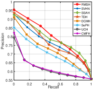
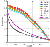
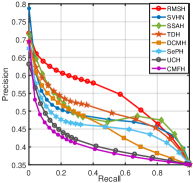
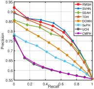
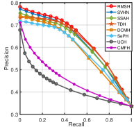
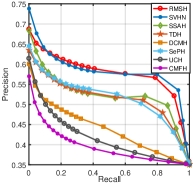
Table 1 reports the NDCG@500 results of compared methods and the precision-recall cures with code length 64 on three datasets are shown in Fig. 3. From Table 1, we observe that our RMSH method substantially outperforms other compared methods on all used datasets. Specifically, compared to the best deep method SVHN, our RMSH obtains the relative increase of 0.2%$\sim$5.86%, 0.1%$\sim$2.58%, and 0.1%$\sim$7.94% with different bits for two cross-modal retrieval tasks on MIRFLICKR25K, NUS-WIDE, and MS COCO datasets, respectively. Because the SVHN method is learning to preserve the binary cross-modal similarity structures, its hashing codes cannot capture the fine-grained ranking information, thus achieve inferior NDCG scores. In contrast, the RMSH learns the more complicated similarity with more robustness to the modality discrepancy and noise. From Fig. 3, we see that the precision-recall evaluations are consistent with the NDCG scores for two cross-modal retrieval tasks. These results re-confirm the superiority of our RMSH method.

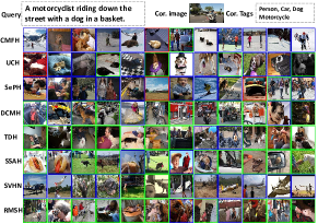
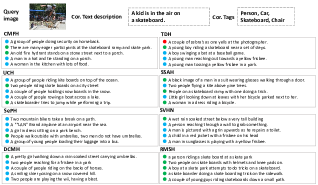
Fig. 4 and Fig. 5 show the ’Text to Image’ and ’Image to Text’ search example of compared methods on COCO dataset. As can be seen, the RMSH method tends to retrieve more relevant images than others for the query containing certain concepts, e.g., person and dog. From Fig. 5, we observe that the RMSH method can roughly capture the similarity across images and text descriptions with multiple tags. Compared to other methods, the top 5 retrieved textual results of RMSH are more meaningful and relevant.

To visualize the quality of learned codes by RMSH, we use t-SNE tools to embed the 128 bits testing binary-like features of NUS-WIDE datasets into 2-dimension spaces and visualize their distribution in Fig. 6. As can be seen, both image and text features provide a better separation between different categories in the common space. Also, the features belonging to the same class from different modalities appear to be compact. These results indicate that the RMSH can preserve not only the multilevel semantic similarity of intra-modal data but also that of the inter-modal data.

4.5 Analysis and Discussion

4.5.1 Impact of robust parameter $\delta$.

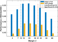
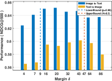
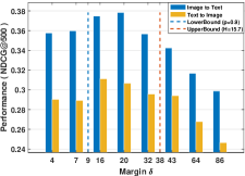
To validate the correctness of the derived bounds of effective robust parameter $\delta$ in Sec. 3.2, we separately tune $\delta$ in $\{K/40$, $K/20$, $K/8$, $3K/20$, $K/4$, $K/3$, $K/2$, $2K/3$ $\}$ with other parameters fixed and report the retrieval performance in Fig. 7, where K=128. We also mark the bounds of effective $\delta$ derived by Eq. (5) and (7) in Fig. 7. We see that the NDCG scores of the RMSH method on all datasets are higher when setting $\delta$ in the range of bounds than when setting it out of the range. This result experimentally proves the correctness of the bounds for more robust cross-modal hash learning.

Besides, Fig. 8 shows the distribution of the Hamming distance of learned codes by RMSH. We observe that 1) too small $\delta$ makes the dissimilar points be nearer, which causes the difficulties of keeping multilevel similarity structure of the similar points; 2) too large $\delta$ prefers to scatter dissimilar points in the whole Hamming space, which is cline to cause false coding since the number of different codes that satisfy the distance constraint is limited.

Table 2: Ablation study of RMSH in terms of NDCG@500 scores on MIRFLICKR25K, NUS-WIDE, and MS COCO datasets. The best result is shown in boldface.

Task	Method	MIRFLICKR25K				NUS-WIDE				MS COCO
		16bits	32bits	64bits	128bits	16bits	32bits	64bits	128bits	16bits	32bits	64bits	128bits
I $\to$ T	RMSH-T	0.4053	0.4202	0.4524	0.4378	0.5437	0.5894	0.5894	0.5885	0.2759	0.3147	0.3430	0.3303
	RMSH-C	0.4066	0.4143	0.4331	0.4597	0.5946	0.6071	0.6383	0.6593	0.1592	0.1811	0.2038	0.2218
	RMSH-P	0.4290	0.4598	0.4920	0.5082	0.6042	0.6235	0.6248	0.6492	0.2918	0.3253	0.3331	0.3155
	RMSH	0.4592	0.4940	0.5180	0.5183	0.6148	0.6401	0.6497	0.6574	0.3037	0.3724	0.3855	0.3998
T $\to$ I	RMSH-T	0.3905	0.4169	0.4061	0.3677	0.5369	0.5560	0.5467	0.5583	0.2575	0.2725	0.2978	0.3079
	RMSH-C	0.3428	0.3696	0.3809	0.4071	0.5467	0.5502	0.5803	0.6069	0.1625	0.1714	0.1868	0.1983
	RMSH-P	0.3912	0.4177	0.4226	0.4453	0.5580	0.5725	0.5723	0.5823	0.2587	0.2747	0.2774	0.2742
	RMSH	0.4379	0.4533	0.4562	0.4628	0.5744	0.5921	0.5900	0.5999	0.2897	0.3080	0.3050	0.3175

4.5.2 Ablation Study.

To analyze the effectiveness of different loss terms and the pseudo-codes network in the proposed RMSH method, we separately remove: the classification loss term $\mathcal{L}_{cl}$, the triplet loss term $\mathcal{L}_{tr}$ and the pseudo-codes with others remained to evaluate their influence on the final performance. These three models are called RMSH-C, RMSH-T, and RMSH-P. Table 2 shows the result. We see that separately removing them will damage the retrieval performance to varying degrees. Notably, 1) the performance gap between RMSH and RMSH-T enlarges with the code length increasing on the MIRFLICKR25K dataset, which confirms the importance of the margin-adaptive triplet loss for preserving the fine-grained similarities of multi-label data in larger Hamming space. 2) As the code length increases on the MIRFLICKR25K and NUS-WIDE datasets, the triplet loss term shows more influence on the final performance than the classification loss term, which indicates that the exploitation of ranking information is more critical than the discriminative information to capture similarity structure. 3) Because the similarity information on the MS COCO dataset (80 concepts) is more sparse, the improvement introduced by the strategy of the pseudo-codes is more significant, i.e., the difference between RMSH and RMSH-P.

Figure 8: The conditional distributions (averaged on the MIRFLICKR25K image test set ) of Hamming distance between testing image codes and training text codes when given semantic similarity, after optimizing RMSH with different robust parameter $\delta$.

Figure 9: Parameter analysis of $\lambda_{1}$, $\lambda_{2}$, $\lambda_{3}$ and $\lambda_{4}$ on MIRFLICKR25K, NUS-WIDE, and COCO dataset.

4.6 Parameter Analysis.

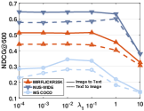
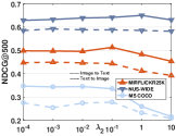
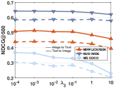
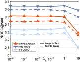
In this section, we conducted the experiments to analyze the parameter sensitive of RMSH on three datasets by varying the one parameter while fixing others. There are mainly four hyper-parameters in RMSH, i.e., $\lambda_{1}$, $\lambda_{2}$, $\lambda_{3}$, and $\lambda_{4}$. The NDCG@500 values with different settings of hyper-parameters in the case of 64 bits on two cross-modal retrieval tasks are summarized in Figure 9. From the figure, 1) we observe that the NDCG scores first obtain a slight increase and then degrades as $\lambda_{1}$ and $\lambda_{2}$ becomes larger, respectively. This indicates that proper $\lambda_{1}$ and $\lambda_{2}$ setting is helpful to preserve intra-modal and inter-modal similarities simultaneously, a huge gap between the value of $\lambda_{1}$ and $\lambda_{2}$ will break this balance and hurt the final performance. 2)The performance emerges decrease when $\lambda_{3}$ gets large since weighing more the classification loss of pseudo-codes will introduce more noise to the optimization process. 3) The result of $\lambda_{4}$ is similar to that of $\lambda_{1}$. A suitable $\lambda_{4}$ is useful to reduce the quantization loss, but a large $\lambda_{4}$ will weaken the goal of preserving similarity.

5 Conclusion

We have presented a novel robust multilevel semantic hashing for multi-label cross-modal retrieval. The approach preserves the multilevel semantic similarity of data and explicitly ensures the distance between different codes is larger than a specific value for robustness to the modality discrepancy. Mainly, we give an effective range of this value from the information coding theory analysis and characterize the above goal as a margin-adaptive triplet loss. We further introduce a pseudo-codes network for the imbalanced semantics. Our approach yields the state-of-the-art empirical results on three benchmarks.

References

- (1) D. Cao, Z. Yu, H. Zhang, J. Fang, L. Nie, Q. Tian, Video-based cross-modal recipe retrieval, in: Proc. ACM MM, 2019, pp. 1685–1693.
- (2) Z. Wang, X. Liu, H. Li, L. Sheng, J. Yan, X. Wang, J. Shao, Camp: Cross-modal adaptive message passing for text-image retrieval, in: Proc. ICCV, 2019, pp. 5764–5773.
- (3) A. Dutta, Z. Akata, Semantically tied paired cycle consistency for zero-shot sketch-based image retrieval, in: Proc. CVPR, 2019, pp. 5089–5098.
- (4) B. Zhu, C.-W. Ngo, J. Chen, Y. Hao, R2gan: Cross-modal recipe retrieval with generative adversarial network, in: Proc. CVPR, 2019, pp. 11477–11486.
- (5) T. Baltrusaitis, C. Ahuja, L. Morency, Multimodal machine learning: A survey and taxonomy, IEEE Trans. Pattern Anal. Mach. Intell. 41 (2) (2019) 423–443.
- (6) R. Xu, C. Li, J. Yan, C. Deng, X. Liu, Graph convolutional network hashing for cross-modal retrieval, in: Proc. IJCAI, 2019, pp. 982–988.
- (7) L. Zhen, P. Hu, X. Wang, D. Peng, Deep supervised cross-modal retrieval, in: Proc. CVPR, 2019, pp. 10394–10403.
- (8) Y. Zhan, J. Yu, Z. Yu, R. Zhang, D. Tao, Q. Tian, Comprehensive distance-preserving autoencoders for cross-modal retrieval, in: Proc. ACM MM, 2018, pp. 1137–1145.
- (9) H. Liu, M. Lin, S. Zhang, Y. Wu, F. Huang, R. Ji, Dense auto-encoder hashing for robust cross-modality retrieval, in: Proc. ACM MM, 2018, pp. 1589–1597.
- (10) Y. Shi, X. You, F. Zheng, S. Wang, Q. Peng, Equally-guided discriminative hashing for cross-modal retrieval, in: Proc. IJCAI, 2019, pp. 4767–4773.
- (11) Q. Jiang, W. Li, Deep cross-modal hashing, in: Proc. CVPR, 2017, pp. 3270–3278.
- (12) J. Wang, T. Zhang, J. Song, N. Sebe, H. T. Shen, A survey on learning to hash, IEEE Trans. Pattern Anal. Mach. Intell. 40 (4) (2018) 769–790.
- (13) P. Hu, X. Wang, L. Zhen, D. Peng, Separated variational hashing networks for cross-modal retrieval, in: Proc. ACM MM, 2019, pp. 1721–1729.
- (14) Y. Cao, B. Liu, M. Long, J. Wang, Cross-modal hamming hashing, in: Proc. ECCV, 2018, pp. 202–218.
- (15) X. Zhang, H. Lai, J. Feng, Attention-aware deep adversarial hashing for cross-modal retrieval, in: Proc. ECCV, 2018, pp. 591–606.
- (16) Z.-D. Chen, Y. Wang, H.-Q. Li, X. Luo, L. Nie, X.-S. Xu, A two-step cross-modal hashing by exploiting label correlations and preserving similarity in both steps, in: Proc. ACM MM, 2019, pp. 1694–1702.
- (17) X. Lu, L. Zhu, Z. Cheng, J. Li, X. Nie, H. Zhang, Flexible online multi-modal hashing for large-scale multimedia retrieval, in: Proc. ACM MM, 2019, pp. 1129–1137.
- (18) C. Li, C. Deng, L. Wang, D. Xie, X. Liu, Coupled cyclegan: Unsupervised hashing network for cross-modal retrieval, in: Proc. AAAI, Vol. 33, 2019, pp. 176–183.
- (19) S. Su, Z. Zhong, C. Zhang, Deep joint-semantics reconstructing hashing for large-scale unsupervised cross-modal retrieval, in: Proc. ICCV, 2019, pp. 3027–3035.
- (20) G. Ding, Y. Guo, J. Zhou, Collective matrix factorization hashing for multimodal data, in: Proc. CVPR, 2014, pp. 2083–2090.
- (21) D. Zhang, W. Li, Large-scale supervised multimodal hashing with semantic correlation maximization, in: Proc. AAAI, 2014, pp. 2177–2183.
- (22) Z. Lin, G. Ding, M. Hu, J. Wang, Semantics-preserving hashing for cross-view retrieval, in: Proc. CVPR, 2015, pp. 3864–3872.
- (23) V. E. Liong, J. Lu, Y. Tan, J. Zhou, Cross-modal deep variational hashing, in: Proc. ICCV, 2017, pp. 4097–4105.
- (24) C. Li, C. Deng, N. Li, W. Liu, X. Gao, D. Tao, Self-supervised adversarial hashing networks for cross-modal retrieval, in: Proc. CVPR, 2018, pp. 4242–4251.
- (25) V. Guruswami, A. Rudra, M. Sudan, Essential coding theory, Draft available at http://www. cse. buffalo. edu/ atri/courses/coding-theory/book.
- (26) H. J. Helgert, R. D. Stinaff, Minimum-distance bounds for binary linear codes, IEEE Trans. Information Theory 19 (3) (1973) 344–356.
- (27) E. Agrell, A. Vardy, K. Zeger, A table of upper bounds for binary codes, IEEE Trans. Information Theory 47 (7) (2001) 3004–3006.
- (28) E. Bellini, E. Guerrini, M. Sala, Some bounds on the size of codes, IEEE Trans. Information Theory 60 (3) (2014) 1475–1480.
- (29) E. N. Gilbert, A comparison of signalling alphabets, The Bell system technical journal 31 (3) (1952) 504–522.
- (30) A. Alfassy, L. Karlinsky, A. Aides, J. Shtok, S. Harary, R. S. Feris, R. Giryes, A. M. Bronstein, Laso: Label-set operations networks for multi-label few-shot learning, in: Proc. CVPR, 2019, pp. 6548–6557.
- (31) D. Wu, Z. Lin, B. Li, M. Ye, W. Wang, Deep supervised hashing for multi-label and large-scale image retrieval, in: Proc. ICMR, 2017, pp. 150–158.
- (32) T. Lin, M. Maire, S. J. Belongie, J. Hays, P. Perona, D. Ramanan, P. Dollár, C. L. Zitnick, Microsoft coco: Common objects in context, in: Proc. ECCV, 2014, pp. 740–755.
- (33) M. J. Huiskes, M. S. Lew, The MIR flickr retrieval evaluation, in: Proceedings of the 1st ACM SIGMM International Conference on Multimedia Information Retrieval, MIR 2008, Vancouver, British Columbia, Canada, October 30-31, 2008, 2008, pp. 39–43.
- (34) T.-S. Chua, J. Tang, R. Hong, H. Li, Z. Luo, Y.-T. Zheng, Nus-wide: A real-world web image database from national university of singapore, in: Proc. of ACM Conf. on Image and Video Retrieval (CIVR’09), July 8-10, 2009.
- (35) K. Järvelin, J. Kekäläinen, Ir evaluation methods for retrieving highly relevant documents, in: International ACM SIGIR Conference on Research and Development in Information Retrieval, 2000, pp. 41–48.
- (36) F. Zhao, Y. Huang, L. Wang, T. Tan, Deep semantic ranking based hashing for multi-label image retrieval, in: Proc. CVPR, 2015, pp. 1556–1564.
- (37) C. Deng, Z. Chen, X. Liu, X. Gao, D. Tao, Triplet-based deep hashing network for cross-modal retrieval, IEEE Trans. Image Processing 27 (8) (2018) 3893–3903.
- (38) K. He, X. Zhang, S. Ren, J. Sun, Deep residual learning for image recognition, in: Proc. CVPR, 2016, pp. 770–778.
- (39) R. Kiros, Y. Zhu, R. Salakhutdinov, R. S. Zemel, R. Urtasun, A. Torralba, S. Fidler, Skip-thought vectors, in: Proc. NeuraIPS, 2015, pp. 3294–3302.