The Hierarchy of Block Models

Abstract

There exist various types of network block models such as the Stochastic Block Model (SBM), the Degree Corrected Block Model (DCBM), and the Popularity Adjusted Block Model (PABM). While this leads to a variety of choices, the block models do not have a nested structure. In addition, there is a substantial jump in the number of parameters from the DCBM to the PABM. The objective of this paper is formulation of a hierarchy of block model which does not rely on arbitrary identifiability conditions. We propose a Nested Block Model (NBM) that treats the SBM, the DCBM and the PABM as its particular cases with specific parameter values, and, in addition, allows a multitude of versions that are more complicated than DCBM but have fewer unknown parameters than the PABM. The latter allows one to carry out clustering and estimation without preliminary testing, to see which block model is really true.

Keywords and phrases: Stochastic Block Model, Degree Corrected Block Model, Popularity Adjusted Block Model, Spectral Clustering, Sparse Subspace Clustering

AMS (2000) Subject Classification: Primary: 62F12, 62H30. Secondary: 05C80

Funding:

Both authors of the paper were partially supported by National Science Foundation (NSF) grants DMS-1712977 and DMS-2014928

1 Introduction

Consider an undirected network with $n$ nodes, no self-loops and multiple edges. Let $A\in\{0,1\}^{n\times n}$ be a symmetric adjacency matrix of the network with $A_{i,j}=1$ if there is a connection between nodes $i$ and $j$, and $A_{i,j}=0$ otherwise. We assume that $A_{i,j}\sim\mbox{Bernoulli}(P_{i,j}),$ $1\leq i<j\leq n,$ where $A_{i,j}$ are conditionally independent given $P_{i,j}$, and $A_{i,j}=A_{j,i}$, $P_{i,j}=P_{j,i}$ for $i>j$. The probability matrix $P$ has low complexity and can be described by a variety of models. One of the ways to address this phenomenon is to assume that all nodes in the network can be partitioned into communities, which are groups that exhibit somewhat similar behavior.

The classical Erdös and Rényi (1959) random graph model assumes that the edges in a random graph are drawn independently with an equal probability and does not allow community structure. The simplest random graph model for networks with community structure is the Stochastic Block Model (SBM) studied by, e.g., Lorrain and White (1971) and Abbe (2018). Under the $K$-block SBM, all nodes are partitioned into communities ${\mathcal{G}}_{k}$, $k=1,\ldots,K$, and the probability of connection between nodes is completely defined by the communities to which they belong: $P_{i,j}=B_{z(i),z(j)}$ where $B_{k,l}$ is the probability of connection between communities $k$ and $l$, and $z\mathrel{\mathop{\mathchar 58\relax}}\{1,...,n\}\to\{1,...,K\}$ is a clustering function such that $z(i)=k$ whenever $i\in{\mathcal{G}}_{k}$. The Erdős-Rényi model can be viewed as the SBM with only one community $K=1$.

Since the real-life networks usually contain a very small number of high-degree nodes while the rest of the nodes have very low degrees, the SBM fails to explain the structure of many networks that occur in practice. The Degree-Corrected Block Model (DCBM), introduced by Karrer and Newman (2011), addresses this deficiency by allowing these probabilities to be multiplied by the node-dependent weights. Under the DCBM, the elements of matrix $P$ are modeled as

$$P_{i,j}=h_{i}B_{z(i),z(j)}h_{j},\quad i,j=1,\ldots,n,$$ (1)

where $h=[h_{1},h_{2},...,h_{n}]$ is a vector of the degree parameters of the nodes, and $B$ is the $(K\times K)$ matrix of baseline interaction between communities. Matrix $B$ and vector $h$ in (1) are defined up to a scalar factor, which is usually fixed via the so called identifiability condition, that can be imposed in a variety of ways. For example, Karrer and Newman (2011) enforce a constraint of the form

$$\sum_{i\in{\mathcal{G}}_{k}}h_{i}=1,\quad k=1,...,K.$$ (2)

The DCBM implies that the probability of connection of a node is uniformly proportional to the degree of this node across all communities. This assumption, however, is violated in a variety of practical applications. For this reason, Sengupta and Chen (2018) introduced the Popularity Adjusted Block Model (PABM). The PABM presents the probability of a connection between nodes as a product of popularity parameters, that depend on the communities to which the nodes belong as well as on the pair of nodes themselves:

$$P_{i,j}=V_{i,z(j)}V_{j,z(i)}.$$ (3)

Although the popularity parameters in (3) are defined up to scalar constants and require an identifiability condition for their recovery, clustering of the nodes and fitting the matrix of connection probabilities do not require any constraints. According to Noroozi et al. (2019), if one re-arranged the nodes, so that the nodes in every community are grouped together, then matrix $P$ of the connection probabilities would appear as $(K\times K)$ block matrix with every block $P^{(k,l)}$, $k,l=1,\ldots,K,$ being of rank one.

Having several types of block models introduces a variety of choices, but also leads to some significant drawbacks. Specifically, although the block models can be viewed as progressively more elaborate with the Erdős-Rényi model being the simplest and the PABM being the most complex, the simpler models cannot be viewed as particular cases of the more sophisticated ones as one paradigm. For this reason, majority of authors carry out estimation and clustering under the assumption that the model which they use is indeed the correct one. There are only very few papers that study goodness of fit in block models setting, and majority of them are concerned with either testing that there are no distinct communities, that is $K=1$ in SBM or DCBM (see, e.g., Banerjee and Ma (2017), Gao and Lafferty (2017) and Jin et al. (2018)), or testing the exact number of communities $K=K_{0}$ in the SBM (see, e.g., Gangrade et al. (2018), Lei (2016) and Mukherjee and Sen (2017)). To the best of our knowledge, Mukherjee and Sen (2017) is the only paper where testing the SBM versus the DCBM is implemented, and the testing in their paper is carried out under rather restrictive assumptions. On the other hand, using the most flexible model, the PABM, may not always be the right choice since there is a substantial jump in complexity from the DCBM with $O(n+K^{2})$ parameters to the PABM with $O(nK)$ parameters.

The objective of the present paper is to provide a unified approach to block models. We would like to point out that we are building a hierarchy of block models, and not a hierarchical stochastic block model. In our paper, we consider a multitude of block models and provide an enveloping nested model that includes them all as particular cases. In what follows, we shall deal only with the graphs where each node belongs to one and only one community, thus, leaving aside the mixed membership models studied by, e.g., Airoldi et al. (2008) and Jin et al. (2017). Specifically, our purpose is formulation of a hierarchy of block models which does not rely on arbitrary identifiability conditions, treats the SBM, the DCBM and the PABM as its particular cases (with specific parameter values) and, in addition, allows a multitude of versions that are more complicated than DCBM but have fewer unknown parameters than the PABM. The aim of this construction is to treat all block models as a part of one paradigm and, therefore, carry out estimation and clustering without preliminary testing to see which block model fits data at hand.

2 The hierarchy of block models

Consider an undirected network with $n$ nodes that are partitioned into $K$ communities ${\mathcal{G}}_{k}$, $k=1,\ldots,K$, by a clustering function $z\mathrel{\mathop{\mathchar 58\relax}}\{1,\ldots,n\}\to\{1,\ldots,K\}$ with the corresponding clustering matrix $Z$. Denote by $B$ the matrix of average connection probabilities between communities, so that for $k,l=1,2,\cdots,K,$ one has

$$B_{k,l}=\frac{1}{n_{k}\,n_{l}}\sum_{i,j=1}^{n}P_{ij}\,I(z(i)=k)\,I(z(j)=l),$$ (4)

where $n_{k}$ is the number of nodes in the community $k$.

In order to better understand the relationships between various block models, consider a rearranged version $P(Z)$ of matrix $P$ where its first $n_{1}$ rows correspond to nodes from class 1, the next $n_{2}$ rows correspond to nodes from class 2, and the last $n_{K}$ rows correspond to nodes from class $K$. Denote the $(k_{1},k_{2})$-th block of matrix $P(Z)$ by $P^{(k_{1},k_{2})}(Z)$. Then, the block models vary by how dissimilar matrices $P^{(k_{1},k_{2})}(Z)$ are. Indeed, under the SBM

$$P^{(k_{1},k_{2})}(Z)=B_{k_{1},k_{2}}1_{n_{k_{1}}}1_{n_{k_{2}}}^{T}$$ (5)

where $1_{k}$ is the $k$-dimensional column vector with all elements equal to one. In the DCBM, there exists a vector $h\in{\mathbb{R}}_{+}^{n}$, with sub-vectors $h^{(k)}\in{\mathbb{R}}_{+}^{n_{k}}$, $k=1,\ldots,K$, such that, for $k_{1},k_{2}=1,2,\cdots,K,$

$$P^{(k_{1},k_{2})}(Z)=B_{k_{1},k_{2}}h^{(k_{1})}(h^{(k_{2})})^{T}.$$ (6)

In the PABM, instead of one vector $h$, there are $K$ vectors $\Lambda^{(1)},\cdots,\Lambda^{(K)}$ with sub-vectors

$$\Lambda^{(k_{1},k_{2})}\in{\mathbb{R}}_{+}^{n_{k_{1}}},\quad k_{1},k_{2}=1,2,\cdots,K.$$ (7)

In this case, vectors $\Lambda^{(k)}$ form the $(n\times K)$ matrix $\Lambda$ with columns partitioned into sub-columns $\Lambda^{(k_{1},k_{2})}$, and

$$P^{(k_{1},k_{2})}(Z)=B_{k_{1},k_{2}}\Lambda^{(k_{1},k_{2})}(\Lambda^{(k_{2},k_{1})})^{T},$$ (8)

for every $k_{1},k_{2}=1,2,\cdots,K$. Hence, (5) and (6) coincide if $h\equiv 1_{n}$, and (8) reduces to (6) if all columns of matrix $\Lambda$ are identical, i.e.

$$\Lambda^{(k_{1},k_{2})}\equiv h^{(k_{1})},\quad k_{1},k_{2}=1,2,\cdots,K.$$ (9)

Since in the DCBM there is only one vector $h$ that models heterogeneity in probabilities of connections, the ratios $P_{i_{1},j}/P_{i_{2},j}$ of the probabilities of connections of two nodes, $i_{1}$ and $i_{2}$, that belong to the same community, are determined entirely by the nodes $i_{1}$ and $i_{2}$ and are independent of the community with which those nodes interact. On the other hand, for the PABM, each node has a different degree of popularity (interaction level) with respect to every other community, so that $P_{i_{1},j_{1}}/P_{i_{2},j_{1}}\neq P_{i_{1},j_{2}}/P_{i_{2},j_{2}}$ if nodes $j_{1}$ and $j_{2}$ belong to different communities. In the PABM, those variable popularities are described by the matrix $\Lambda\in[0,1]^{n\times K}$ which reduces to a single vector $h$ in the case of the DCBM. One can easily imagine the situation where nodes do not exhibit different levels of activity with respect to every community but rather with respect to some groups of communities, “meta-communities”, so that there are $L$, $1\leq L\leq K$, different vectors $H^{(l)}\in{\mathbb{R}}_{+}^{n},\quad l=1,2,\cdots,L,$ and each of columns $\Lambda_{k}$, $k=1,2,\cdots,K$, of matrix $\Lambda$ is equal to one of vectors $H^{(l)}$. In other words, there exists a clustering function $c\mathrel{\mathop{\mathchar 58\relax}}\{1,...,K\}\to\{1,...,L\}$ with the corresponding clustering matrix $C$ such that

$$\Lambda_{k}=H^{(l)},\ l=c(k),\ l=1,\ldots,L,\ k=1,\ldots,K.$$

We name the resulting model the Nested Block Model (NBM) to emphasize that the model is equipped with the nested structure that allows to obtain a multitude of popular block models as its particular cases.

3 The Nested Stochastic Block Model (NBM)

The NBM contains two types of communities, the regular communities that can be distinguished by the average probabilities of connections between them (like in the SBM or the DCBM) and the meta-communities that are described by the distinct patterns of probabilities of connections of individual nodes across the communities.

Observe that both concepts are quite natural. Indeed, in random network models, specifically in assortative network models that are most common, communities are usually loosely defined as groups of nodes that have higher probability of connection than the rest. In our case, we retain the notion and define communities as groups of nodes with a specific (average) probability of connection between them. The meta-communities refer to the node-to-community specific connection weights. In DCBM, each node has only one specific weight to account for the difference in connection probabilities with the rest; in PABM, the weights can be different for any node and community pair. In our nested model, we allow some of the node-to-community interactions have the same patterns for a group of communities, the meta-communities.

For instance, consider an example of College of Sciences of a university that includes Departments of Biology, Chemistry, Mathematics, Physics, Psychology, Sociology, and Statistics. Each of the departments forms a natural community, and the average density of connections is much higher within the communities than between them. However, one can naturally partition College of Sciences into meta-communities of natural sciences (Biology, Chemistry, and Physics), social sciences (Psychology and Sociology) and mathematics and data sciences (Mathematics and Statistics). For example, faculty in mathematics and data sciences who are working on various problems in astronomy, genetics, dynamical systems, or theory of chemical reactions will have high probability of connections with the natural sciences meta-community. On the other hand, those who are involved in, for example, studying social interactions, monitoring cyber and homeland security, or relationships between countries, will have more dense interactions with the social sciences meta-community. While one can use the PABM and model interactions between each pair of the departments separately, the patterns within meta-communities may be similar enough that using the most complex PABM with $O(nK)$ parameters may not be justified.

Note that the meta-communities introduced in this paper should not be mixed with the mega-communities considered in Wakita and Tsurumi (2007) and Li et al. (2020). The difference between the present paper and the above cited publications is that in Wakita and Tsurumi (2007) and Li et al. (2020) the mega-communities are determined by intermediate results of the clustering algorithms while we define the meta-communities on the basis of the distinct patterns of the connection probabilities of nodes with respect to different communities. Our approach is also very different from the hierarchical stochastic block model studied in, e.g., Li et al. (2020) or Lyzinski et al. (2017). In those papers, the authors examine SBMs with a large number of communities, that can be partitioned into groups based on some similarities in the matrix of block probabilities. We, on the other hand, deal with more diverse block models, for which the SBM is the simplest one. In addition, the authors in Lyzinski et al. (2017) impose assumptions that require the SBM to be very strongly assortative. Hence, the only common feature between our paper and the above mentioned ones is that there exist groups of communities; everything else is completely different.

For any $M$ and $K\leq M$, denote by ${\mathcal{M}}_{M,K}$ the collection of all clustering matrices $Z\in\{0,1\}^{M\times K}$ with the corresponding clustering function $z\mathrel{\mathop{\mathchar 58\relax}}\{1,\ldots,M\}\to\{1,\ldots,K\}$ such that $Z_{i,k}=1$ iff $z(i)=k$, $i=1,\ldots,M$. Then, $Z^{T}Z=\mbox{diag}(n_{1},\ldots,n_{K})$ where $n_{k}$ is the size of community $k$, $k=1,\ldots,K$. The NBM, with $K$ communities and $L\leq K$ meta-communities, is defined by two clustering matrices $Z\in{\mathcal{M}}_{n,K}$ and $C\in{\mathcal{M}}_{K,L}$ with corresponding clustering functions $z$ and $c$ that, respectively, partition the $n$ nodes into $K$ communities, and $K$ communities into $L$ meta-communities. If the $l$-th meta-community consists of $K_{l}$ communities and the community sizes are $n_{k}$, then the total number of nodes in meta-community $l$ is $N_{l}$, where

$$N_{l}=\sum_{k=1}^{K}n_{k}\,I(c(k)=l),\quad\sum_{l=1}^{L}K_{l}=K,\quad\sum_{l=1}^{L}N_{l}=n,\quad l=1,\cdots,L.$$ (10)

The communities are characterized by their average connection probability matrix, with elements $B_{k_{1},k_{2}}$, $k_{1},k_{2}=1,2,\ldots,K$, defined in (4). In order to better understand the meta-communities, consider a permutation matrix $\mathscr{P}_{Z,C}$ that arranges nodes into communities consecutively, and orders communities so that the $K_{l}$ blocks within the $l$-th meta-community are consecutive, $l=1,2,\ldots,L$. Recall that $\mathscr{P}_{Z,C}$ is an orthogonal matrix with $\mathscr{P}_{Z,C}^{-1}=\mathscr{P}_{Z,C}^{T}$ and denote

$$P(Z,C)=\mathscr{P}_{Z,C}^{T}\,P\,\mathscr{P}_{Z,C},\quad P=\mathscr{P}_{Z,C}\,P(Z,C)\,\mathscr{P}_{Z,C}^{T}.$$

According to $Z$ and $C$, matrix $P$ is partitioned into $K^{2}$ blocks $P^{(k_{1},k_{2})}(Z,C)\in[0,1]^{n_{k_{1}}\times n_{k_{2}}}$, $k_{1},k_{2}=1,\ldots,K$, with the block-averages given by (4). In addition, blocks $P^{(k_{1},k_{2})}(Z,C)$ can be combined into the $L^{2}$ meta-blocks

$$\tilde{P}^{(l_{1},l_{2})}(Z,C)\in[0,1]^{N_{l_{1}}\times N_{l_{2}}},$$

corresponding to probabilities of connections between meta-communities $l_{1}$ and $l_{2}$, $l_{1},l_{2}=1,\ldots,L$.

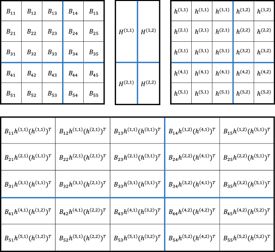
Figure 1: Matrices associated with the NBM with $K=5$, $L=2$, $K_{1}=3$, $K_{2}=2$. Bold lines identify the meta-blocks. Top left: matrix $B$ partitioned into blocks $B^{(l_{1},l_{2})}$. Top, middle: matrix $H$. Top right: matrix $H$ with columns expressed via vectors $h^{(k,l)}$ and repeated: column 1- $K_{1}$ times; column 2 - $K_{2}$ times. Bottom: the probability matrix with $K^{2}$ blocks and $L^{2}$ meta-blocks.

Consider matrix $H\in{\mathbb{R}}_{+}^{n\times L}$ (Figure 1, top middle), where each column $H_{l}$, $l=1,\ldots,L$, can be partitioned into $K$ sub-vectors $h^{(k,l)}\in{\mathbb{R}}_{+}^{n_{k}}$ of lengths $n_{k}$, $k=1,\ldots,K$. Those sub-vectors are combined into $L$ meta sub-vectors ${H}^{(m,l)}\in{\mathbb{R}}_{+}^{N_{m}}$ of lengths $N_{m}$, $m=1,\cdots,L$, according to matrix $C$, where $N_{m}$ is defined in (10). Similarly, matrix $B\in[0,1]^{K\times K}$ of block probabilities is partitioned into sub-matrices $B^{(l_{1},l_{2})}\in[0,1]^{K_{l_{1}}\times K_{l_{2}}}$, $l_{1},l_{2}=1,\cdots,L$. With these notations, for any $l_{1},l_{2}=1,\cdots,L$, the $(l_{1},l_{2})$-th meta-block of $P$ can be presented as

$$\tilde{P}^{(l_{1},l_{2})}(Z,C)=\left({H}^{(l_{1},l_{2})}({H}^{(l_{2},l_{1})})^{T}\right)\circ\left(J^{(l_{1})}B^{(l_{1},l_{2})}(J^{(l_{2})})^{T}\right),$$ (11)

where $A\circ B$ is the Hadamard product of $A$ and $B$, and matrices $J^{(l)}\in\{0,1\}^{N_{l}\times K_{l}}$, $l=1,\ldots,L$, are of the form

$${\small J^{(l)}=\begin{bmatrix}1_{n_{k_{1}}}&\boldsymbol{0}&\cdots&\boldsymbol{0}\\ \boldsymbol{0}&1_{n_{k_{2}}}&\cdots&\boldsymbol{0}\\ \vdots&\vdots&\cdots&\vdots\\ \boldsymbol{0}&\boldsymbol{0}&\cdots&1_{n_{k_{K_{l}}}}\\ \end{bmatrix}.}$$ (12)

By rewriting (11) in an equivalent form, one can conclude that each of the meta-blocks $\tilde{P}^{(l_{1},l_{2})}(Z,C)$ (and, hence, $\tilde{P}^{(l_{1},l_{2})}$ if we scramble them to the original order) follows the (non-symmetric) DCBM model with $K_{l_{1}}\times K_{l_{2}}$ blocks. Specifically, for a pair of sub-vectors $H^{(l_{1},l_{2})}\in{\mathbb{R}}_{+}^{N_{l_{1}}}$ and $H^{(l_{2},l_{1})}\in{\mathbb{R}}_{+}^{N_{l_{2}}}$ of matrix $H$ and a matrix $B^{(l_{1},l_{2})}\in[0,1]^{K_{l_{1}}\times K_{l_{2}}}$ containing average probabilities of connections for each pair of communities within the meta-community $(l_{1},l_{2})$ one has

$$\tilde{P}^{(l_{1},l_{2})}(Z,C)=Q^{(l_{1},l_{2})}J^{(l_{1})}B^{(l_{1},l_{2})}(J^{(l_{2})})^{T}Q^{(l_{2},l_{1})}.$$

Here, $Q^{(l_{1},l_{2})}=\mbox{diag}(H^{(l_{1},l_{2})})$ and the $(k_{1},k_{2})$-th block of $P(Z,C)$ is given by

$$P^{(k_{1},k_{2})}(Z,C)=B_{k_{1},k_{2}}h^{(k_{1},l_{2})}\left(h^{(k_{2},l_{1})}\right)^{T},\quad l_{i}=c(k_{i}),\ i=1,2,$$ (13)

where $h^{(k,l)}\in{\mathbb{R}}_{+}^{n_{k}}$ is a sub-vector of $H^{(m,l)}$ with $m=c(k)$. Observe that the formulation above imposes a natural scaling on the sub-vectors $h^{(k,l)}$ of $H$, since it follows from equations (4) and (13), that for any pair of communities $(k_{1},k_{2})$ which belong to a pair of meta-communities $(l_{1},l_{2})$, one has

$$n_{k_{1}}\,n_{k_{2}}\ B_{k_{1},k_{2}}=1_{k_{1}}^{T}\,P^{(k_{1},k_{2})}(Z,C)\,1_{k_{2}}=B_{k_{1},k_{2}}\left(1_{k_{1}}^{T}h^{(k_{1},l_{2})}\right)\,\left(1_{k_{2}}^{T}\,h^{(k_{2},l_{1})}\right).$$ (14)

The latter implies that for any $k=1,\ldots,K$ and $l=1,\ldots,L$,

$$1_{k}^{T}h^{(k,l)}=n_{k},\quad k=1,\ldots,K,\ l=1,\ldots,L.$$ (15)

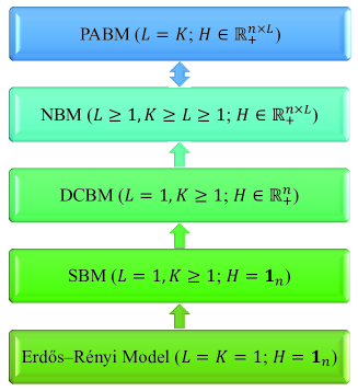
Figure 2: The hierarchy of block models

Now, it is easy to see that all block models, the SBM, the DCBM and the PABM, can be viewed as particular cases of the NBM introduced above. Indeed, the DCBM is a particular case of the NBM with $L=1$ while the PABM corresponds to the setting of $L=K$. Finally, due to (15), the SBM constitutes a particular case of the NBM with $L=1$ and matrix $H$ reduced to vector $1_{n}$, the $n$-dimensional column vector with all entries equal to one. Moreover, the absence of the community structure (whether in the SBM or the DCBM) is equivalent to $K=1$, and implies that the NBM necessarily reduces to the DCBM. This one-community DCBM is indeed just the Chung-Lu model introduced in Chung and Lu (2002).

Remark 1.

The case of unconnected communities.   Note that equations (13) and (14) become identities for any vectors $h^{(k_{1},l_{2})}$ and $h^{(k_{2},l_{1})}$ if $B_{k_{1},k_{2}}=0$, $c(k_{1})=l_{1}$ and $c(k_{2})=l_{2}$, which happens if matrix $P^{(k_{1},k_{2})}(Z,C)$ is identically equal to zero. In this case, there are two possibilities. If there exists $\tilde{k}_{2}$ with $c(\tilde{k}_{2})=l_{2}$ such that $B_{k_{1},\tilde{k}_{2}}\neq 0$, then set $h^{(k_{1},l_{2})}=h^{(k_{1},c(\tilde{k}_{2}))}$. If no such $\tilde{k}_{2}$ exists (which corresponds to the case when the whole row of matrix $B^{l_{1},l_{2})}$ is equal to zero), then set $h^{(k_{1},l_{2})}=1_{n_{k_{1}}}$. The latter can be interpreted as an understanding that, if all nodes in community $k_{1}$ are not connected to nodes in meta-community $l_{2}$, they are “equally unconnected”.

Observe that treating zero elements of matrix $B$ in this manner leads to the smallest number of meta-communities and, hence, to the smallest number of parameters in the model. For example, in the extreme case when matrix $B$ is diagonal, one obtains that matrix $H$ has only one column, $L=1$ and the NBM just reduces to DCBM.

4 Optimization procedure for estimation and clustering

Note that, in terms of the matrices $J^{(l)}$ defined in (12), the scaling conditions (15) appear as

$$(J^{(l)})^{T}\,Q^{(l,l^{\prime})}\,J^{(l)}=(J^{(l)})^{T}\,J^{(l)},\ l,l^{\prime}=1,...,L.$$ (16)

Let $\mathscr{P}_{\widehat{Z},\widehat{C}}$ be the permutation matrix corresponding to estimated clustering matrices $\widehat{Z}\in{\mathcal{M}}_{n,\hat{K}}$ and $\widehat{C}\in{\mathcal{M}}_{\hat{K},\hat{L}}$. Consider the set $\Im(n,K,L)$ of matrices $\Theta$ with blocks $\Theta^{(l_{1},l_{2})}\in[0,1]^{N_{l_{1}}\times N_{l_{2}}}$, $l_{1},l_{2}=1,...,L,$ such that conditions (10) and (16) hold and

$$\Theta=\bigcup_{l_{1},l_{2}}\Theta^{(l_{1},l_{2})},\,\Theta^{(l_{1},l_{2})}=Q^{(l_{1},l_{2})}J^{(l_{1})}B^{(l_{1},l_{2})}(J^{(l_{2})})^{T}Q^{(l_{2},l_{1})},$$

$$B^{(l_{1},l_{2})}\in[0,1]^{K_{l_{1}}\times K_{l_{2}}},\,Q^{(l_{1},l_{2})}\in{\mathcal{D}}_{l_{1}},$$ (17)

$$Z\in{\mathcal{M}}_{n,K},\ C\in{\mathcal{M}}_{K,L},\,l_{1},l_{2}=1,...,L,$$

where ${\mathcal{D}}_{m}$ the set of diagonal matrices with diagonals in ${\mathbb{R}}_{+}^{m}$. Then, it is easy to see that $P=\mathscr{P}_{Z,C}^{T}\,\Theta\,\mathscr{P}_{Z,C}$, so its estimator can be obtained as

$$\hat{P}=\mathscr{P}_{\widehat{Z},\widehat{C}}\ \widehat{\Theta}(\widehat{Z},\widehat{C})\ \mathscr{P}_{\widehat{Z},\widehat{C}}^{T}.$$ (18)

Here, for given values of $K$ and $L$, $(\widehat{Z},\widehat{C},\widehat{\Theta})$ is a solution of the following optimization problem

$${\small(\widehat{Z},\widehat{C},\widehat{\Theta})\in\underset{Z,C,\Theta}{\text{argmin}}\left\|A(Z,C)-\Theta\right\|_{F}^{2}}$$ (19)

subject to conditions $A(Z,C)=\mathscr{P}_{Z,C}^{T}\,A\,\mathscr{P}_{Z,C}$, (10), (16) and (17). In real life, however, the values of $K$ and $L$ are unknown and need to be incorporated into the optimization problem by adding a penalty $\mbox{Pen}(K,L)$ on $K$ and $L$:

$$(\widehat{\Theta},\widehat{Z},\widehat{C},\hat{K},\hat{L})\in\underset{Z,C,K,L,\Theta}{\text{argmin}}\left\{\left\|A(Z,C)-\Theta\right\|_{F}^{2}+\mbox{Pen}(K,L)\right\},$$ (20)

where optimization is carried out subject to conditions $A(Z,C)=\mathscr{P}_{Z,C}^{T}A\mathscr{P}_{Z,C}$, (10), (16) and (17). After that, the estimator $\hat{P}$ of $P_{*}$ can be obtained as (18). The penalty in (20) should account for the difficulty of estimating $nL+K^{2}$ unknown parameters ($nL$ entries in matrix $H$ and $K^{2}$ entries in matrix $B$) and uncertainty of clustering which is of the logarithmic order $n\ln K$ of the cardinality of the set of clustering matrices. For this reason, we choose the penalty of the form

$$\mbox{Pen}(K,L)=C_{1}(nL+K^{2})\ln n+C_{2}n\ln K$$ (21)

where $C_{1}$ and $C_{2}$ are absolute constants. The logarithmic factor $\ln n$ in (21) is due to the proof technique and, can possibly be removed.

In practice, one would need to solve optimization problem (19) for each $K=1,...,n,$ and $L=1,\ldots,K$, and then find the values $(\hat{K},\hat{L})$ that minimize the right hand side in (20). After that, the estimator $\hat{P}$ of $P$ is obtained as (18). Then, the following statement holds.

Theorem 1.

Let Assumptions A1 and A2 hold. Let $(\widehat{\Theta},\widehat{Z},\widehat{C},\hat{K},\hat{L})$ be a solution of optimization problem (20) subject to conditions $A(Z,C)=\mathscr{P}_{Z,C}^{T}A\mathscr{P}_{Z,C}$, (10), (16) and (17) with the penalty given by (21). Then, for the estimator $\hat{P}$ given by (18), the true matrix $P_{*}$, any $K$, $L$, $Z\in{\mathcal{M}}_{n,K}$, $C\in{\mathcal{M}}_{K,L}$ and any matrix $P=\mathscr{P}_{Z,C}\Theta\mathscr{P}_{Z,C}^{T}$ with $\Theta\in\Im(n,K,L)$, one has

$${\mathbb{P}}\left\{\|\hat{P}-P_{*}\|_{F}^{2}\leq 3\big{[}\|P-P_{*}\|_{F}^{2}+\mbox{Pen}(K,L)\big{]}\right\}\geq 1-(n^{2}\log_{2}n+1)e^{-n/32},$$

$${\mathbb{E}}\|\hat{P}-P_{*}\|_{F}^{2}\leq 3\big{[}\|P-P_{*}\|_{F}^{2}+\mbox{Pen}(K,L)\big{]}+n^{5}e^{-n/32}.$$

Solution of optimization problem (20) requires a search over the continuum of matrices $\Theta\in\Im(n,K,L)$. In order to simplify the estimation, we consider a solution of a more straightforward optimization problem. It is easy to observe (see Figure 1) that each of the block columns of matrix $P$ is a matrix of rank one and, given the clustering, it can be obtained by the rank one projection of the respective adjacency sub-matrix. Denote the block columns of the re-arranged matrices $P$ and $A$ by $P^{(l,k)}(Z,C)$ and $A^{(l,k)}(Z,C)$. Then, the optimization problem appears as

$$(\widehat{Z},\widehat{C},\hat{K},\hat{L})\in\underset{Z,C,K,L}{\text{argmin}}\Bigg{\{}\sum_{l=1}^{L}\sum_{k=1}^{K}\left\|A^{(l,k)}(Z,C)-\Pi_{(1)}\left(A^{(l,k)}(Z,C)\right)\right\|_{F}^{2}+\overline{\mbox{Pen}}(K,L)\Bigg{\}}$$ (22)

$$\text{s.t.}\ A(Z,C)=\mathscr{P}_{Z,C}^{T}A\mathscr{P}_{Z,C},$$

where $\Pi_{(1)}\left(A^{(l,k)}(Z,C)\right)$ is the rank one projection of the matrix $A^{(l,k)}(Z,C)$. Then, $\widehat{\Theta}$ is the block matrix with blocks $\widehat{\Theta}^{(l,k)}=\Pi_{(1)}\left(A^{(l,k)}(\widehat{Z},\widehat{C})\right)$, $l=1,\cdots,\hat{L},\ k=1,\cdots,\hat{K}$. Note that the new formulation requires estimation of the larger number of parameters $(nK+K^{2})$ versus $(nL+K^{2})$ in (20), so the new penalty is of the form

$$\overline{\mbox{Pen}}(K,L)=\Psi_{1}nK+\Psi_{2}K^{2}\ln n+\Psi_{3}n\ln K,$$ (23)

where $\Psi_{1}$, $\Psi_{2}$, and $\Psi_{3}$ are positive absolute constants.

Theorem 2.

Let Assumptions A1 and A2 hold. Let $(\widehat{\Theta},\widehat{Z},\widehat{C},\hat{K},\hat{L})$ be a solution of optimization problem (22) with $\overline{\mbox{Pen}}(K,L)$ of the form (23). Then, for the estimator $\hat{P}$ of $P_{*}$ given by (18) and any $t>0$, one has

$${\mathbb{P}}\left\{\left\|\hat{P}-P_{*}\right\|_{F}^{2}\leq\tilde{C}\,[\overline{\mbox{Pen}}(n,K_{*},L_{*})+t]\right\}\geq 1-3e^{-t},$$

$${\mathbb{E}}\left\|\hat{P}-P_{*}\right\|_{F}^{2}\leq\tilde{C}\,[\overline{\mbox{Pen}}(n,K_{*},L_{*})+3].$$

Here $K_{*}$ and $L_{*}$ are the true number of communities and meta-communities and

$$\tilde{C}=\tilde{C}(\Psi_{1},\Psi_{2},\Psi_{3})>0$$

is an absolute constant.

Observe that Theorem 2 delivers smaller error rates if $K_{*}/L_{*}\ll\ln n$, i.e., if $n$ is large. In addition, for known values of $K$ and $L$, one needs to carry optimization in (22) only over the set of clustering matrices. In this sense, optimization problem (22) can be viewed as a kind of modularity optimization which has been used for estimation and clustering in the SBM (Bickel and Chen (2009)), the DCBM (Zhao et al. (2012)) and the PABM (Sengupta and Chen (2018)). The deficiency of this sort of approach is that it is NP-hard and requires some replacement by a computationally viable method. In our case, this relaxation is provided by a subspace clustering which allows us to find the clustering matrix $C$ and hence detect the meta-communities. Subsequently, we detect the communities within meta-communities using spectral clustering. We describe those procedures in detail in the next section.

5 Detectability of communities and meta-communities

As we have mentioned above, in what follows, we focus on the optimization problem (22). Observe that the viability of the NBM introduced above relies on the correct detection of communities and meta-communities. In order to assess identifiability of clustering matrices $Z$ and $C$, consider a noiseless model where one can observe the probability matrix $P_{*}$ instead of the adjacency matrix $A$. Indeed, if matrices $Z$ and $C$ can be correctly recovered (up to permutation of columns), then matrix $B$ can be obtained by averaging the probabilities in $P_{*}(Z,C)$ using formula (14). Furthermore, it follows from (11) that sub-columns $H^{(l_{1},l_{2})}$ of matrix $H$ can be obtained by applying rank one approximations to the Hadamard quotient of $\tilde{P}^{(l_{1},l_{2})}(Z,C)$ and $J^{(l_{1})}B^{(l_{1},l_{2})}(J^{(l_{2})})^{T}$.

One however does not need to identify all those quantities in order to estimate clustering matrices $Z$ and $C$. Optimization problem (22) suggests that matrices $Z$ and $C$ can be obtained just on the basis of modularity optimization based on the partitions of the adjacency matrix. In order to confirm that the communities and meta-communities are detectable, we assume that $K=K_{*}$ and $L=L_{*}$ are known and impose the following assumptions:

A1.  Matrix $B$ is non-singular with the smallest singular value bounded away from zero: $\lambda_{\min}(B)\geq\lambda_{0}>0.$

A2.   For each $k=1,\cdots,K$, vectors $h^{(k,l)}$, $l=1,\cdots,L$, are linearly independent.

Under those assumptions, it is easy to see that the meta-columns of matrix $P_{*}$, corresponding to the $l$-th meta-community, lie in the distinct linear subspace $S_{l}$ of the dimension $K_{*}$ with the basis defined by $K$ distinct combinations of sub-vectors $h^{(k,l)}$, $k=1,...,K_{*}$. For this reason, one can find meta-communities by identifying those subspaces. Subsequently, for finding communities within meta-communities, one notes that the $l$-th diagonal block of the probability matrix $\tilde{P}^{(l,l)}(Z_{*},C_{*})$ in (11), corresponding to the $l$-th meta-community, $l=1,...,L$, follows the DCBM model. Due to Assumption A2, matrix $B^{(l,l)}$ in (11) is of full rank, which guarantees identifiability of communities in the meta-community $l$. Specifically, the following statement is true:

Lemma 1.

Let Assumptions A1 and A2 hold. Let $K=K_{*}$ and $L=L_{*}$ be known. Let $Z_{*}\in{\mathcal{M}}_{n,K}$ and $C_{*}\in{\mathcal{M}}_{K,L}$ be the true clustering matrices, while $Z\in{\mathcal{M}}_{n,K}$ and $C\in{\mathcal{M}}_{K,L}$ be arbitrary clustering matrices. Then,

$$\sum_{l=1}^{L}\sum_{k=1}^{K}\left\|P_{*}^{(l,k)}(Z_{*},C_{*})\right. \left.-\ \Pi_{(1)}\left(P_{*}^{(l,k)}(Z_{*},C_{*})\right)\right\|_{F}^{2}$$ (24)

$$\leq\sum_{l=1}^{L}\sum_{k=1}^{K}\left\|P_{*}^{(l,k)}(Z,C)-\Pi_{(1)}\left(P_{*}^{(l,k)}(Z,C)\right)\right\|_{F}^{2}$$

where, for any matrix $B$, $\Pi_{(1)}(B)$ is its rank one approximation. Moreover, equality in (24) occurs if and only if matrices $Z$ and $Z_{*}$, $C$ and $C_{*}$ coincide up to a permutation of columns.

Lemma 1 ensures that, if the optimization problem (22) is applied to the true probability matrix with known $K$ and $L$, then the true clustering matrices $Z_{*}$ and $C_{*}$ will be recovered up to the permutation of columns. However, since optimization procedures in (20) and (22) are NP-hard, they cannot be implemented in practice.

6 Implementation of clustering

In this section, we describe a computationally tractable clustering procedure that can replace optimization procedures in (20) and (22). Since the model requires identification of meta-communities and regular communities, naturally, the clustering is carried out in two steps. First, we find the clustering matrix $C$ that arranges the nodes into $L$ meta-communities. Subsequently, we detect communities within each of the meta-communities, obtaining the clustering matrix $Z$.

In order to accomplish the first task, we observe that, under Assumptions A1 and A2, the meta-columns of matrix $P$, corresponding to the $l$-th meta-community, lie in the distinct linear subspace $S_{l}$ of the dimension $K$ with the basis defined by $K$ distinct combinations of subvectors $h^{(k,l)}$, $k=1,...,K$. For this reason, one can find meta-communities by identifying those subspaces. This can be done by subspace clustering, the technique which has been well developed by the computer vision community. Subsequently, for finding communities within meta-communities, one notes that the probability matrix of each meta-community follows the non-symmetric DCBM model, for which there exist several clustering methods.

Subspace clustering is designed for separation of points that lie in the union of subspaces. Let $\{X_{j}\in\mathbb{R}^{D}\}_{j=1}^{n}$ be a given set of points drawn from an unknown union of $K\geqslant 1$ linear or affine subspaces $\{S_{i}\}_{i=1}^{K}$ of unknown dimensions $d_{i}=\text{dim}(S_{i})$, $0<d_{i}<D$, $i=1,...,K$. In the case of linear subspaces, the subspaces can be described as $S_{i}=\{{\mbox{$x$}}\in\mathbb{R}^{D}\mathrel{\mathop{\mathchar 58\relax}}{\mbox{$x$}}={\mbox{$U$}}_{i}{\mbox{$y$}}\}$, $i=1,...,K,$ where ${\mbox{$U$}}_{i}\in\mathbb{R}^{D\times d_{i}}$ is a basis for subspace $S_{i}$ and ${\mbox{$y$}}\in\mathbb{R}^{d_{i}}$ is a low-dimensional representation for point $x$. The goal of subspace clustering is to find the number of subspaces $K$, their dimensions $\{d_{i}\}_{i=1}^{K}$, the subspace bases $\{{\mbox{$U$}}_{i}\}_{i=1}^{K}$, and the segmentation of the points according to the subspaces.

Several methods have been developed to implement subspace clustering such as algebraic methods (Boult and Gottesfeld Brown (1991), Ma et al. (2008), Vidal et al. (2005)), iterative methods (Agarwal and Mustafa (2004), Bradley and Mangasarian (2000), Tseng (2000)), and self representation based methods (Elhamifar and Vidal (2009), Elhamifar and Vidal (2013), Favaro et al. (2011), Liu et al. (2013), Liu et al. (2010), Soltanolkotabi et al. (2014), Vidal (2011)).

In this paper we use the self-representation type method, the Sparse Subspace Clustering (SSC) developed by Elhamifar and Vidal (2013). The technique is based on representation of each of the vectors as a sparse linear combination of all other vectors, with the expectation that a vector is more likely to be represented as a linear combination of vectors in its own subspace rather than other subspaces. The weights obtained by this procedure are used to form the affinity matrix which, in turn, is partitioned using the spectral clustering methods.

If matrix $P_{*}$ were known, the weight matrix $W$ would be based on writing every data point as a sparse linear combination of all other points by minimizing the number of nonzero coefficients

$$\mathop{\text{missing}}{min}_{W_{j}}\left\|W_{j}\right\|_{0}\quad\mbox{s.t.}\quad(P_{*})_{j}=\sum_{k\neq j}W_{k,j}(P_{*})_{k}$$ (25)

where, for any matrix $B$, $B_{j}$ is its $j$-th column. The affinity matrix of the SSC is the symmetrized version of the weight matrix $W$. Note that since, due to Assumption A2, the subspaces are linearly independent, the solution to the optimization problem (25) is $W_{j}$ such that $W_{k,j}\neq 0$ only if points $k$ and $j$ are in the same subspace. Since the problem (25) is NP-hard, one usually solves its convex LASSO relaxation

$$\mathop{\text{missing}}{min}_{W_{j}}\left\|W_{j}\right\|_{1}\quad\mbox{s.t.}\quad(P_{*})_{j}=\sum_{k\neq j}W_{k,j}(P_{*})_{k}$$ (26)

In the case of data contaminated by noise, the SSC algorithm does not attempt to write data as an exact linear combination of other points and replaces (26) by penalized optimization. Specifically, in our simulations, we solve the elastic net problem

$$\widehat{W}_{j}\in\underset{W_{j}}{\text{argmin}}\left\{\Big{[}0.5\left\|{A_{j}-AW_{j}}\right\|_{2}^{2}+\gamma_{1}\left\|W_{j}\right\|_{1}\right.\left.+\gamma_{2}\left\|W_{j}\right\|_{2}^{2}\Big{]}\ \mbox{s.t.}\ W_{j,j}=0\right\},\ j=1,\ldots,n,$$ (27)

where $\gamma_{1},\gamma_{2}>0$ are tuning parameters. The quadratic term stabilizes the LASSO problem by making the problem strongly convex. We solve (27) using a fast version of the LARS algorithm implemented in SPAMS Matlab toolbox Mairal et al. (2014). Given $\widehat{W}$, the clustering matrix $C$ is then obtained by applying spectral clustering to the affinity matrix $|\widehat{W}|+|\widehat{W}^{T}|$, where, for any matrix $B$, matrix $|B|$ has absolute values of elements of $B$ as its entries. Algorithm 1 summarizes the SSC procedure described above.

The correctness of the SSC relies on the so called self-expressiveness property (SEP), which guarantees that each column of the probability matrix $P_{*}$ will be represented using columns of its own subspace rather than columns of the other subspaces. The latter leads to the $n\times n$ estimated matrix of weights $\widehat{W}$ where $\widehat{W}_{i,j}=0$ if nodes $i$ and $j$ are in different meta-communities. Subsequently, according to Algorithm 1, one applies spectral clustering to the symmetrized matrix of weights $|\widehat{W}|+|\widehat{W}^{T}|$. It is easy to see that, if the true matrix of probabilities $P_{*}$ were available, then, under Assumptions A1 and A2, matrix $\widehat{W}$ obtained as a solution of (25) or (26), satisfies the SEP. Since matrix $A$ is generated on the basis of matrix $P_{*}$, one expects that the entries of matrix $\widehat{W}$, obtained as a solution of (27), are equal to zero for pairs of nodes that belong to different meta-communities. Although the latter fact is supported by simulations, the formal proof of this statement is very nontrivial and is not presented in this paper.

1 Input: Adjacency matrix $A$, number of meta-communities $L$, tuning parameters $\gamma_{1},\gamma_{2}$

2 Output: Clustering matrix $C$

3 Steps:

4 1: For $j=1,...,n$, find $\widehat{W}_{j}$ in (27)

2: Apply spectral clustering to the affinity matrix $|\widehat{W}|+|\widehat{W}^{T}|$ to find clustering matrix $C$

Algorithm 1  The SSC procedure

Once the meta-communities are discovered, one needs to detect communities inside of each meta-community. Recall that each meta-community follows the non-symmetric DCBM. One of the popular clustering methods for the DCBM is the weighted $k$-median algorithm used in Lei and Rinaldo (2015) and Gao et al. (2018). Algorithm 2 follows Gao et al. (2018). For the known number of communities $K$, the algorithm starts with estimating the probability matrix $P$ by the best rank $K$ approximation of the adjacency matrix, obtaining $\hat{P}=UDU^{T}$, where $U\in{\mathbb{R}}^{n\times K}$ contains $K$ leading eigenvectors and $D$ is a diagonal matrix of top $K$ eigenvalues. After that, the columns of $\hat{P}$ are normalized, leading to $\tilde{P}_{i}=\hat{P}_{i}/\|\hat{P}_{i}\|_{1}$, $i=1,2,\ldots,n$. Finally, the $k$-median algorithm is applied to $\tilde{P}$ to find the community assignment.

1 Input: Adjacency matrix $A\in\{0,1\}^{n\times n}$, number of clusters $k$

2 Output: Community assignment

3 Steps:

4 1: Find $\hat{P}=UDU^{T}$ with $U\in{\mathbb{R}}^{n\times K}$, the best rank $k$ approximation of matrix $A$

5 2: For $j=1,...,n$, find $\tilde{P}_{j}=\hat{P}_{j}/\|\hat{P}_{j}\|_{1}$

3: Apply $k$-median algorithm to $\tilde{P}$ to obtain community assignment

Algorithm 2  Spectral clustering with $k$-median

In the first step of clustering, we apply Algorithm 1 to the adjacency matrix $A$ to find $L$ meta-communities defined by the clustering matrix $C$. In the second step, Algorithm 2 is applied to each of $L$ meta-communities, obtained at the first step. Specifically, we apply Algorithm 2 with $k=K_{l}$ and $n=N_{l}$ to cluster the $l$-th meta-community, $l=1,...,L$. The union of these communities combined with the clustering matrix $C$, yields the clustering matrix $Z$. We elaborate on the implementation of this two-step clustering procedure in Section 7.1.

Remark 2.

Finding the number of communities and meta-communities.   In theory, in order to find the unknown values of $K$ and $L$, one needs to solve optimization problem (20) or (22) for each $K=1,...,n$ and $L=1,\ldots,K$, and then find the values $(\hat{K},\hat{L})$ that minimize the right hand side in (20) or (22). In practice, however, the constants in the penalties are too large and will lead to significant underestimation of the number of communities and meta-communities. For this reason, in practice, one should run optimization with several small values of $L$ (say, $L=1,2,3$). For each of the values of $L$, one finds the meta-communities using SSC (Algorithm 1). As soon as the meta-communities are identified, each of those meta-communities follow the DCBM, hence, the problem reduces to finding the number of communities in those DCBMs. Several authors tackled this problem, see, e.g., Ma et al. (2019). Subsequently, one can choose the number of meta-communities using a common complexity penalty such as AIC or BIC.

Remark 3.

Alternative way of clustering.   Under the assumptions of the paper, if the SSC was applied to the matrix $P_{*}$ instead of the adjacency matrix $A$, it would yield $W_{i,j}=0$ when nodes $i$ and $j$ are in the same meta-community but different communities. Hence, it is possible to reverse the procedure and first cluster nodes into the communities using the SSC and then, subsequently cluster the communities into the meta-communities. However, since clustering is carried out on the basis of matrix $A$, and the meta-communities are in general larger than communities (and there are fewer of them), the procedure used in the paper is more precise and stable, so that the estimated weights are more likely to satisfy the self-expressiveness property (SEP).

7 Simulations and a real data example

7.1 Simulations on synthetic networks

In the experiments with synthetic data, we generate networks with $n$ nodes, $L$ meta-communities and $K$ communities that fit the NBM. For simplicity, we consider perfectly balanced networks where the number of nodes in each community and meta-community are respectively $n/K$ and $n/L$, and there are $K/L$ communities in each meta-community. First, we generate $L$ distinct $n$-dimensional random vectors with entries between 0 and 1. To this end, we generate a random vector $Y\in(0,1)^{n}$ and partition it into $K$ blocks $Y^{(k)}$, $k=1,...,K$, of size $n/K$. The vector $\bar{h}^{(1)}$ is generated from $Y$ by sorting each block of $Y$ in ascending order. After that, we partition each of the $K$ blocks, $\bar{h}^{(k,1)}$ of $\bar{h}^{(1)}$, into $L$ sub-blocks $\bar{h}^{(k,1)}_{i}$, $i=1,...,L$, of equal size. To generate the $k$-th block $\bar{h}^{(k,2)}$ of $\bar{h}^{(2)}$, we reverse the order of entries in each sub-block $\bar{h}^{(k,1)}_{i}$ and rearrange them in descending order. The blocks $\bar{h}^{(k,s)}$ of subsequent vectors $\bar{h}^{(s)}$, $s=3,...,L$, are formed by re-arranging the order of sub-blocks $\bar{h}^{(k,2)}_{i}$ in each sub-vector $\bar{h}^{(k,2)}$. The $L$ vectors $\bar{h}^{(l)}$, $l=1,...,L$, generated by this procedure have different patterns leading to detectable meta-communities. Subsequently, we scale the vectors as $H^{(k,l)}=(n/K)\,\bar{h}^{(k,l)}/\|\bar{h}^{(k,l)}\|_{1}$, $k=1,...,K$, $l=1,...,L$, obtaining matrix $H$. After that, we replicate $K/L$ times each of the columns of $H$ (Figure 1, top right) and denote the resulting matrix by $\tilde{H}$. Matrix $B$ has entries

$$B_{k,l}=\tilde{B}_{k,l}\left[(\tilde{H}_{max})_{k,l}\right]^{-2},\quad k,l=1,...,K,$$ (28)

where $\tilde{B}$ is a $(K\times K)$ symmetric matrix with random entries between 0.35 and 1 to avoid very sparse networks, and the largest entries of each row (column) are on the diagonal. Matrix $\tilde{H}_{max}$ is a $K\times K$ symmetric matrix defined as

$$(\tilde{H}_{max})_{k,l}=\max\left(\tilde{H}^{(k,l)},\tilde{H}^{(l,k)}\right),\quad k,l=1,...,K,$$

where $\tilde{H}^{(k,l)}$ is the $(k,l)$-th block of matrix $\tilde{H}$. The term $\left[(\tilde{H}_{max})_{k,l}\right]^{-2}$ in (28) guarantees that the entries of probability matrix $P(Z,C)$ do not exceed one. To control how assortative the network is, we multiply the off-diagonal entries of $B$ by the parameter $\omega\in(0,1)$. The values of $\omega$ close to zero produce an almost block diagonal probability matrix $P(Z,C)$ while the values of $\omega$ close to one lead to $P(Z,C)$ with more diverse entries. We obtain the probability matrix $P(Z,C)$ as

$$P^{(k,l)}(Z,C)=B_{k,l}\,\tilde{H}^{(k,l)}\left(\tilde{H}^{(l,k)}\right)^{T},\ k,l=1,...,K.$$

After that, to obtain the probability matrix $P$, we generate random clustering matrices $Z\in{\mathcal{M}}_{n,K}$ and $C\in{\mathcal{M}}_{K,L}$ and their corresponding $n\times n$ permutation matrices $\mathscr{P}(Z)$ and $\mathscr{P}(C)$, respectively. Subsequently, we set $\mathscr{P}_{Z,C}=\mathscr{P}(Z)\mathscr{P}(C)$ and obtain the probability matrix $P$ as $P=\mathscr{P}_{Z,C}P(Z,C)(\mathscr{P}_{Z,C})^{T}$. Finally we generate the lower half of the adjacency matrix $A$ as independent Bernoulli variables $A_{i,j}\sim\text{Bern}(P_{i,j})$, $i=1,\ldots,n,j=1,\ldots,i-1$, and set $A_{i,j}=A_{j,i}$ when $j>i$. In practice, the diagonal $\text{diag}(A)$ of matrix $A$ is unavailable, so we estimate matrix $P$ without its knowledge.

We apply Algorithm 1 to find the clustering matrix $\widehat{C}$. Since the diagonal elements of matrix $A$ are unavailable, we initially set $A_{i,i}=0$, $i=1,...,n$. We use $\gamma_{1}=30\rho(A)$ and $\gamma_{2}=125(1-\rho(A))$ where $\rho(A)$ is the density of matrix $A$, the proportion of nonzero entries in $A$. The spectral clustering in step 2 of the Algorithm 1 is carried out by the normalized cut algorithm of Shi and Malik (2000). Once the meta-communities are obtained, we apply Algorithm 2 to detect communities inside each meta-community. The union of detected communities and the clustering matrix $\widehat{C}$ yields the clustering matrix $\widehat{Z}$. Given $\widehat{Z}$ and $\widehat{C}$, we generate matrix $A(\widehat{Z},\widehat{C})=\mathscr{P}_{\widehat{Z},\widehat{C}}^{T}\,A\,\mathscr{P}_{\widehat{Z},\widehat{C}}$ with blocks $A^{(k,l)}(\widehat{Z},\widehat{C})$, $k=1,\ldots,K$, $l=1,\ldots,L$, and obtain $\widehat{\Theta}^{(k,l)}(\widehat{Z},\widehat{C})$ by using the rank one projection for each of the blocks. Finally, we estimate matrix $P$ by $\hat{P}$, given by formula (18).

	DCBM: $K=6$ , $L=1$
	$n=900$		$n=1260$
	$\omega=0.6$	$\omega=0.8$	$\omega=0.6$	$\omega=0.8$
PABM: Clust. Err.	0.82411 (0.00221)	0.82378 (0.00210)	0.82696 (0.00176)	0.82725 (0.00179)
DCBM: Clust. Err.	0.07326 (0.01389)	0.12241 (0.03542)	0.05302 (0.01040)	0.08989 (0.02555)
NBM: Clust. Err.	0.07326 (0.01389)	0.12241 (0.03542)	0.05302 (0.01040)	0.08989 (0.02555)
PABM: Est. Err.	0.00885 (0.00089)	0.00761 (0.00065)	0.00808 (0.00076)	0.00693 (0.00078)
DCBM: Est. Err.	0.00212 (0.00016)	0.00274 (0.00023)	0.00153 (0.00010)	0.00196 (0.00015)
NBM: Est. Err.	0.00203 (0.00010)	0.00237 (0.00014)	0.00146 (0.00006)	0.00167 (0.00009)
	NBM: $K=6$ , $L=2$
	$n=900$		$n=1260$
	$\omega=0.6$	$\omega=0.8$	$\omega=0.6$	$\omega=0.8$
PABM: Clust. Err.	0.43885 (0.03879)	0.45456 (0.02452)	0.42849 (0.05346)	0.47122 (0.04774)
DCBM: Clust. Err.	0.38644 (0.02658)	0.46126 (0.05912)	0.39413 (0.01859)	0.45976 (0.05440)
NBM: Clust. Err.	0.04737 (0.01193)	0.09207 (0.02935)	0.03458 (0.01208)	0.07601 (0.03838)
Communities
NBM: Clust. Err.	0.00026 (0.00086)	0.00004 (0.00020)	0.00458 (0.00759)	0.00071 (0.00177)
Meta-Communities
PABM: Est. Err.	0.00487 (0.00040)	0.00507 (0.00033)	0.00397 (0.00049)	0.00390 (0.00048)
DCBM: Est. Err.	0.00518 (0.00084)	0.00788 (0.00146)	0.00492 (0.00055)	0.00733 (0.00101)
NBM: Est. Err.	0.00237 (0.00012)	0.00284 (0.00019)	0.00182 (0.00027)	0.00201 (0.00011)
	NBM: $K=6$ , $L=3$
	$n=900$		$n=1260$
	$\omega=0.6$	$\omega=0.8$	$\omega=0.6$	$\omega=0.8$
PABM: Clust. Err.	0.36722 (0.07693)	0.46137 (0.04546)	0.40421 (0.05570)	0.45825 (0.04972)
DCBM: Clust. Err.	0.28004 (0.06783)	0.45044 (0.10014)	0.27603 (0.06227)	0.44704 (0.08994)
NBM: Clust. Err.	0.07400 (0.03607)	0.06941 (0.04866)	0.08807 (0.03832)	0.09074 (0.07109)
Communities
NBM: Clust. Err.	0.05104 (0.03903)	0.00856 (0.02127)	0.07598 (0.04009)	0.02564 (0.03323)
Meta-Communities
PABM: Est. Err.	0.00536 (0.00074)	0.00637 (0.00090)	0.00452 (0.00053)	0.00507 (0.00114)
DCBM: Est. Err.	0.00586 (0.00073)	0.00936 (0.00125)	0.00501 (0.00069)	0.00826 (0.00118)
NBM: Est. Err.	0.00363 (0.00072)	0.00338 (0.00074)	0.00318 (0.00070)	0.00288 (0.00078)
	PABM: $K=6$ , $L=6$
	$n=900$		$n=1260$
	$\omega=0.6$	$\omega=0.8$	$\omega=0.6$	$\omega=0.8$
PABM: Clust. Err.	0.08059 (0.02294)	0.03141 (0.02969)	0.05667 (0.02857)	0.02376 (0.04287)
DCBM: Clust. Err.	0.20037 (0.01484)	0.22489 (0.01141)	0.19725 (0.01416)	0.21728 (0.01119)
NBM: Clust. Err.	0.08059 (0.02294)	0.03141 (0.02969)	0.05667 (0.02857)	0.02376 (0.04287)
PABM: Est. Err.	0.00434 (0.00021)	0.00463 (0.00107)	0.00308 (0.00057)	0.00325 (0.00099)
DCBM: Est. Err.	0.00475 (0.00074)	0.00790 (0.00089)	0.00438 (0.00051)	0.00732 (0.00090)
NBM: Est. Err.	0.00433 (0.00020)	0.00463 (0.00107)	0.00307 (0.00057)	0.00325 (0.00099)

Table 1: The clustering errors $\mbox{Err}(\widehat{Z},Z)$, $\mbox{Err}(\widehat{C},C)$, and estimation error $\Delta(\hat{P})$ given by (30), for model fitting using the DCBM, the NBM and the PABM, under correctly and incorrectly specified models. The networks are generated under three different models: the DCBM (with $K=6$, $L=1$), the NBM (with $K=6$, $L=2$ and 3), and the PABM (with $K=6$, $L=6$), for $n=900$ and 1260 and $\omega=0.6$ and 0.8. The results are evaluated over 30 simulation runs. The corresponding standard deviations are given in parentheses.

For evaluation of the performance of our method, we generate networks from three different models: the DCBM (with $K=6$, $L=1$), the NBM (with $K=6$, $L=2$ and 3), and the PABM (with $K=6$, $L=6$), for $n=900$ and $n=1260$ and $\omega=0.6$ and $\omega=0.8$. Then we fit the DCBM, the NBM, and the PABM to each of the generated networks. The proportion of misclassified nodes (clustering error) is evaluated as

$$\mbox{Err}(Z,\widehat{Z})=(2n)^{-1}\,\underset{\mathscr{P}_{K}\in\mathcal{P}_{K}}{\min}\|Z\mathscr{P}_{K}-\widehat{Z}\|_{F}^{2}$$ (29)

where $\mathcal{P}_{K}$ is the set of permutation matrices $\mathscr{P}_{K}\mathrel{\mathop{\mathchar 58\relax}}\{1,...,K\}\to\{1,...,K\}$. Table 1 shows the accuracy of clustering for fitting correct and incorrect models to the generated networks. For all settings, the clustering errors of fitting the correct model are smaller than those of the incorrect ones. Moreover, in the NBM, since meta-communities are detected first, the accuracy of detecting $K$ communities depends on the precision of detecting $L$ meta-communities. One can see from Table 1 that, when the NBM is the true model, there is a significant improvement in the accuracy of detecting $K$ communities using the two-step clustering procedure, with finding the meta-communities being the key task. It is also worth noting that when DCBM is the true model of the networks, then there is only one meta-community. Hence, when NBM is fitted to the networks, there is no need to detect meta-communities (as there is only one). Hence, we just detect communities by applying Algorithm 2, which leads to the results identical to the ones obtained by fitting the true model (DCBM). Similarly, when the true model of the network is PABM, there is only one community inside of each meta-community. Thus, when NBM is fitted to the networks, one only needs to detect meta-communities using Algorithm 1, attaining the same results as the ones obtained by fitting the true model (PABM).

Since the model with larger number of parameters allows for a more accurate estimation of matrix $P$, we measure the accuracy of an estimator $\hat{P}$ of $P$ by the squared Frobenius norm of their difference with the added AIC-type penalty

$$\Delta(\hat{P})=n^{-2}\left\{\|\hat{P}-P\|_{F}^{2}+2\bar{P}\ N_{Par}\right\}.$$ (30)

Here, $\|{\hat{P}-P}\|_{F}^{2}$ acts as a pseudo likelihood, $\bar{P}=n^{-2}\sum_{i,j=1}^{n}P_{ij}$ is the average density of $P$, and $N_{Par}$ is the number of parameters in a model: $N_{Par}=n+K(K+1)/2-1$ for the DCBM, $N_{Par}=nL+K(K+1)/2-KL$ for the NBM, and $N_{Par}=nK$ for the PABM. In DCBM, $\hat{P}$ is obtained by solving a low rank approximation problem, as it is explained in Gao et al. (2018). In the PABM, $\hat{P}$ is found by the post-clustering estimation, which is based on rank one approximations (see Noroozi et al. (2019)). Table 1 shows that, even if the AIC penalty on the number of parameters is added, correctly fitted models have smaller estimation error (30) than incorrectly fitted ones.

Thus, the results in Table 1 can be summarized as follows. If the true model is NBM, then NBM fits best and the other models fit rather poorly. On the other hand, if the true model is DCBM (or PABM), then DCBM (or PABM) fits best, but NBM also fits well, with accuracy not much worse than the true model. Therefore, without knowledge of the true model (as it happens in real-world scenarios), fitting NBM is the safest option.

7.2 Real data examples

         

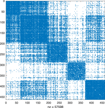
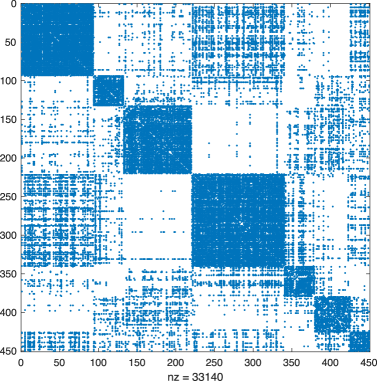
Figure 3: The adjacency matrices of the butterfly similarity network with 57598 nonzero entries and 5 clusters (left) and the brain network with 33140 nonzero entries and 7 clusters (right) after clustering

In this section, we describe application of the two-step clustering procedure of Section 6 to two real life networks, a butterfly similarity network and a human brain network.

We consider the butterfly similarity network extracted from the Leeds Butterfly dataset Wang et al. (2018), which contains fine-grained images of 832 butterfly species that belong to 10 different classes, with each class containing between 55 and 100 images. In this network, the nodes represent butterfly species and edges represent visual similarities (ranging from 0 to 1) between them, evaluated on the basis of butterfly images. We extract the five largest classes and draw an edge between two nodes if the visual similarity between them is greater than zero, obtaining a simple graph with 462 nodes and 28799 edges. We carry out clustering of the nodes, employing the two-step clustering procedure, first finding $L=4$ meta-communities by Algorithm 1, and then using Algorithm 2 to find communities within meta-communities. We conclude that the first meta-community has two communities, while the other three meta-communities have one community each. We also applied Algorithms 1 and 2 separately for detection of five communities. Here, Algorithms 1 and 2 correspond, respectively, to the PABM and the DCBM settings with $K=5$. Subsequently, we compare the clustering assignments with the true class specifications of the species. Algorithms 1 and 2 lead to 74% and 77% accuracy, respectively, while the two-step clustering procedure provides better 84% accuracy, thus, justifying the application of the NBM. The better results are due to the higher flexibility of the NBM.

The second example deals with analysis of a human brain functional network, based on the brain connectivity dataset, derived from the resting-state functional MRI (rsfMRI) Crossley et al. (2013). In this dataset, the brain is partitioned into 638 distinct regions and a weighted graph is used to characterize the network topology. For a comparison, we use the Asymptotical Surprise method Nicolini et al. (2017) which is applied for clustering the GroupAverage rsfMRI matrix in Crossley et al. (2013). Asymptotical Surprise detects 47 communities with sizes ranging from 1 to 133. Since the true clustering as well as the true number of clusters are unknown for this dataset, we treat the results of the Asymptotical Surprise as the ground truth. In order to generate a binary network, we set all nonzero weights to one in the GroupAverage rsfMRI matrix, obtaining a network with 18625 undirected edges. For our study, we extract 7 largest communities derived by the Asymptotical Surprise, obtaining a network with 450 nodes and 16570 edges. Similarly to the previous example, we apply Algorithms 1 and 2 separately to detect seven communities, obtaining, respectively, 88% and 73% accuracy. We also use the the two-step clustering procedure above, detecting six meta-communities and seven communities, attaining 92% accuracy.

Figure 3 shows the adjacency matrices of the butterfly similarity network (left) and the human brain network (right) after clustering.

8 Discussion

The present paper examines the hierarchy of block models with the purpose of treating all existing singular-membership block models as a part of one formulation, which is free from arbitrary identifiability conditions. The blocks differ by the average probability of connections and can be combined into meta-blocks that have common heterogeneity patterns in the connection probabilities.

The hierarchical formulation proposed above (see Figure 2) can be utilized for a variety of purposes. Since the NBM treats all other block models as its particular cases, one can carry out estimation and clustering without assuming that a specific block model holds, by employing the NBM with $K$ communities and $L$ meta-communities, where both $K$ and $L$ are unknown. The values of $K$ and $L$ can later be derived on the basis of penalties. Furthermore, in the framework above, one can easily test one block model versus another. For instance, $L=K$ suggests the PABM while $L=1$ implies the DCBM. If, additionally, $H=1_{n}$, then DCBM reduces to SBM. Finally, one can see from Figure 2 that the absence of distinct communities ($K=1$) always leads to DCBM, which reduces to Erdős-Rényi model if $H=1_{n}$.

9 Proofs

9.1 Proof of Theorem 1.

Let $\Xi=A-P_{*}$. We let $\mathscr{P}_{Z,C,K,L}$ denote the permutation matrix that arranges meta-blocks consecutively and also blocks all meta-blocks consecutively. For simplicity, let

$$\mathscr{P}\equiv\mathscr{P}_{Z,C,K,L},\hskip 2.84526pt\mathscr{P}_{*}\equiv\mathscr{P}_{Z_{*},C_{*},K_{*},L_{*}},\hskip 2.84526pt\hat{\mathscr{P}}\equiv\mathscr{P}_{\hat{Z},\hat{C},\hat{K},\hat{L}}$$

For any matrix $S$, denote

$$S(Z,C,K,L)=\mathscr{P}_{Z,C,K,L}^{T}S\mathscr{P}_{Z,C,K,L}$$ (31)

Then, for any $Z,C,K,$ and $L$:

$$\left\|\hat{\mathscr{P}}^{T}A\hat{\mathscr{P}}-\hat{\Theta}(\hat{Z},\hat{C},\hat{K},\hat{L})\right\|_{F}^{2}+\mbox{Pen}(n,\hat{K},\hat{L})\leq\left\|\mathscr{P}^{T}A\mathscr{P}-\mathscr{P}^{T}P\mathscr{P}\right\|_{F}^{2}+\mbox{Pen}(n,K,L)$$

Therefore,

$$\left\|A-\hat{\mathscr{P}}\hat{\Theta}(\hat{Z},\hat{C},\hat{K},\hat{L})\hat{\mathscr{P}}^{T}\right\|_{F}^{2}+\mbox{Pen}(n,\hat{K},\hat{L})\leq\left\|A-P\right\|_{F}^{2}+\mbox{Pen}(n,K,L)$$

or

$$\left\|A-\hat{P}\right\|_{F}^{2}+\mbox{Pen}(n,\hat{K},\hat{L})\leq\left\|A-P\right\|_{F}^{2}+\mbox{Pen}(n,K,L).$$ (32)

Subtracting and adding $P_{*}$ in the norms in both sides of (32), we rewrite it as

$$\left\|\hat{P}-P_{*}\right\|_{F}^{2}\leq\left\|P-P_{*}\right\|_{F}^{2}+2\langle\Xi,\hat{P}-P\rangle+\mbox{Pen}(n,K,L)-\mbox{Pen}(n,\hat{K},\hat{L}).$$ (33)

Denote

$$P_{0}(K,L)=\underset{P\in\Im(n,K,L)}{\text{inf}}\left\|P-P_{*}\right\|_{F}^{2},$$

$$(K_{0},L_{0})=\underset{K,L}{\text{inf}}\left\{\left\|P_{0}(K,L)-P_{*}\right\|_{F}^{2}+\mbox{Pen}(n,K,L)\right\}.$$

Then, for $\hat{P}\equiv\hat{P}(\hat{K},\hat{L})$ and $P_{0}\equiv P_{0}(K_{0},L_{0})$, one has

$$\left\|\hat{P}-P_{*}\right\|_{F}^{2}\leq\left\|P_{0}-P_{*}\right\|_{F}^{2}+2\langle\Xi,P_{*}-P_{0}\rangle$$ (34)

$$2\langle\Xi,\hat{P}-P_{*}\rangle+\mbox{Pen}(n,K_{0},L_{0})-\mbox{Pen}(n,\hat{K},\hat{L}).$$

Denote

$$\tau(n,K,L)= n\ln K+K\ln L+(K^{2}+2nL)\ln\left(9nL\right)$$ (35)

and consider two sets $\Omega$ and $\Omega^{c}$

$$\Omega=\left\{\omega\mathrel{\mathop{\mathchar 58\relax}}\left\|\hat{P}-P_{*}\right\|_{F}\geq C_{0}2^{s_{0}}\sqrt{\tau(n,K_{0},L_{0})}\right\},$$ (36)

$$\Omega^{c}=\left\{\omega\mathrel{\mathop{\mathchar 58\relax}}\left\|\hat{P}-P_{*}\right\|_{F}\leq C_{0}2^{s_{0}}\sqrt{\tau(n,K_{0},L_{0})}\right\}$$

where $s_{0}$ is a constant. If $\omega\in\Omega^{c}$, then

$$\left\|\hat{P}-P_{*}\right\|_{F}^{2}\leq C_{0}^{2}2^{2s_{0}}\tau(n,K_{0},L_{0})$$ (37)

Consider the case when $\omega\in\Omega$. It follows from Hoeffding inequality that, for any fixed matrix $G$, any $\alpha>0$ and any $t>0$ one has

$${\mathbb{P}}\left\{2\langle\Xi,G\rangle\geq\alpha\left\|G\right\|_{F}^{2}+2t/\alpha\right\}\leq e^{-t}.$$ (38)

Then, there exists a set $\tilde{\Omega}_{t}$ such that $P(\tilde{\Omega}_{t})\geq 1-e^{-t}$ and for $\omega\in\tilde{\Omega}_{t}$

$$2\langle\Xi,P_{*}-P_{0}\rangle\leq\alpha\left\|P_{*}-P_{0}\right\|_{F}^{2}+2t/\alpha$$ (39)

Note that the set $\Omega$ can be partitioned as $\Omega=\underset{K,L}{\bigcup}\Omega_{K,L}$, where

$$\Omega_{K,L}=\bigg{\{}\omega\mathrel{\mathop{\mathchar 58\relax}} \Big{(}\left\|\hat{P}-P_{*}\right\|_{F}\geq C_{0}2^{s_{0}}\sqrt{\tau(n,K_{0},L_{0})}\Big{)}\hskip 2.84526pt\cap\hskip 2.84526pt(\hat{K}=K,\hskip 2.84526pt\hat{L}=L)\bigg{\}}$$ (40)

with $\Omega_{K_{1},L_{1}}\cap\Omega_{K_{2},L_{2}}=\emptyset$ unless $K_{1}=K_{2}$ and $L_{1}=L_{2}$. Denote

$$\Delta(n,K,L)=C_{0}^{2}C_{2}\tau(n,K,L)+n,$$ (41)

where $\tau(n,K,L)$ is defined in (35). Then,

$${\mathbb{P}}\bigg{\{}\Big{[}2\langle\Xi,\hat{P}(n,\hat{K},\hat{L})-P_{*}\rangle-\frac{1}{2}\left\|\hat{P}(n,\hat{K},\hat{L})-P_{*}\right\|_{F}^{2}-2\Delta(n,\hat{K},\hat{L})\Big{]}\geq 0\bigg{\}}$$

$$\leq\sum_{K=1}^{n}\sum_{L=1}^{K}{\mathbb{P}}\bigg{\{}\underset{\hat{P}\in\Omega_{K,L}}{\text{sup}}\Big{[}2\langle\Xi,\hat{P}-P_{*}\rangle-\frac{1}{2}\left\|\hat{P}-P_{*}\right\|_{F}^{2}-2\Delta(n,K,L)\Big{]}\geq 0\bigg{\}}$$

By Lemma 4 in Section 9.4, there exist sets $\tilde{\Omega}_{K,L}\subseteq\Omega_{K,L}\subset\Omega$ such that ${\mathbb{P}}(\tilde{\Omega}_{K,L}^{c})\leq\log_{2}n\cdot\exp{(-n\cdot 2^{2s_{0}-7})}$ and, for $\omega\in\tilde{\Omega}_{K,L}$, one has

$$\Big{\{}2\langle\Xi,\hat{P}-P_{*}\rangle\leq\frac{1}{2}\left\|\hat{P}-P_{*}\right\|_{F}^{2}+2\Delta(n,K,L)\Big{\}}\cap\Big{\{}\hat{K}=K,\hskip 2.84526pt\hat{L}=L\Big{\}}$$

Denote

$$\tilde{\Omega}=\left(\underset{K,L}{\cap}\tilde{\Omega}_{K,L}\right)\cap\tilde{\Omega}_{t}$$ (42)

and observe that

$${\mathbb{P}}\left(\tilde{\Omega}\right)\geq 1-n^{2}\log_{2}n\cdot\exp{(-n\cdot 2^{2s_{0}-7})}-e^{-t}.$$

Then, for $\omega\in\tilde{\Omega}$, one has

$$2\langle\Xi,\hat{P}-P_{*}\rangle\leq\frac{1}{2}\left\|\hat{P}-P_{*}\right\|_{F}^{2}+2\Delta(n,\hat{K},\hat{L})$$ (43)

and it follows from (39) with $\alpha=1/2$ that

$$2\langle\Xi,P_{*}-P_{0}\rangle\leq\frac{1}{2}\left\|P_{*}-P_{0}\right\|_{F}^{2}+4t$$ (44)

Plugging (43) and (44) into (LABEL:eq:main_err_klopp), obtain that for $\omega\in\tilde{\Omega}$ one has

$$\left\|\hat{P}-P_{*}\right\|_{F}^{2}\leq\left\|P_{0}-P_{*}\right\|_{F}^{2}+\mbox{Pen}(n,K_{0},L_{0})+\frac{1}{2}\left\|\hat{P}-P_{*}\right\|_{F}^{2}+$$

$$2\Delta(n,\hat{K},\hat{L})+\frac{1}{2}\left\|P_{*}-P_{0}\right\|_{F}^{2}+4t-\mbox{Pen}(n,\hat{K},\hat{L})$$

Finally, setting

$$\mbox{Pen}(n,K,L)=2\Delta(n,K,L)=2\left[C_{0}^{2}\tau(n,K,L)+n\right],$$

obtain that for any $t>0$, for $\omega\in\tilde{\Omega}$, one has

$$\left\|\hat{P}-P_{*}\right\|_{F}^{2}\leq 3\left\|P_{0}-P_{*}\right\|_{F}^{2}+2\mbox{Pen}(n,K_{0},L_{0})+8t,$$

for any $\omega\in\Omega$. Now, for $\omega\in\Omega^{c}$, it follows from (37) that

$$\left\|\hat{P}-P_{*}\right\|_{F}^{2}\leq C_{0}^{2}2^{2s_{0}}\tau(n,K_{0},L_{0})\leq 2^{2s_{0}-1}\mbox{Pen}(n,K_{0},L_{0})$$

Setting $s_{0}=1$ and $t=n/32$, obtain

$${\mathbb{P}}\bigg{\{}\left\|\hat{P}-P_{*}\right\|_{F}^{2}\leq\Big{[}3\left\|P_{0}-P_{*}\right\|_{F}^{2}+2\mbox{Pen}(n,K_{0},L_{0})\Big{]}+\frac{n}{4}\bigg{\}}\geq 1-(n^{2}\log_{2}n+1)e^{-\frac{n}{32}},$$

so that

$${\mathbb{P}}\bigg{\{}\left\|\hat{P}-P_{*}\right\|_{F}^{2}\leq 3\underset{P\in\Im(n,K,L)}{\text{inf}}\Big{[}\left\|P-P_{*}\right\|_{F}^{2}+\mbox{Pen}(n,K,L)\Big{]}\bigg{\}}\geq 1-(n^{2}\log_{2}n+1)e^{-\frac{n}{32}}$$

Since $\left\|\hat{P}-P_{*}\right\|_{F}^{2}\leq n^{2}$, obtain

$${\mathbb{E}}\left\|\hat{P}-P_{*}\right\|_{F}^{2}\leq 3\underset{P\in\mathscr{M}(n,K,L)}{\text{min}}\Big{[}\left\|P-P_{*}\right\|_{F}^{2}+\mbox{Pen}(n,K,L)\Big{]}+n^{5}e^{-n/32}$$

9.2 Proof of Theorem 2.

Let

$$F_{1}(n,K,L)=C_{1}nK+C_{2}K^{2}\ln(ne)+C_{3}(\ln n+(n+1)\ln K+K\ln L)$$

$$F_{2}(n,K,L)=2\ln n+2(n+1)\ln K+2K\ln L,$$

where $C_{1},$ $C_{2},$ and $C_{3}$ are absolute constants. Denote $\Xi=A-P_{*}$ and recall that, given matrix $P_{*}$, entries $\Xi_{i,j}=A_{i,j}-(P_{*})_{ij}$ of $\Xi$ are the independent Bernoulli errors for $1\leq i\leq j\leq n$ and $A_{i,j}=A_{j,i}$. Then, following notation (31), for any $Z$, $C$, $K$, and $L$

$$\Xi(Z,C,K,L)=\mathscr{P}^{T}\Xi\mathscr{P}$$

$$P_{*}(Z,C,K,L)=\mathscr{P}^{T}P_{*}\mathscr{P},$$

where $\mathscr{P}\equiv\mathscr{P}_{Z,C,K,L}$. Then it follows from (22) that

$$\left\|\hat{\mathscr{P}}^{T}A\hat{\mathscr{P}}-\hat{\Theta}(\hat{Z},\hat{C},\hat{K},\hat{L})\right\|_{F}^{2}+\mbox{Pen}(n,\hat{K},\hat{L})\leq\left\|\mathscr{P}_{*}^{T}A\mathscr{P}_{*}-\mathscr{P}_{*}^{T}P_{*}\mathscr{P}_{*}\right\|_{F}^{2}+\mbox{Pen}(n,K_{*},L_{*})$$

where $\mathscr{P}_{*}\equiv\mathscr{P}_{Z_{*},C_{*},K_{*},L_{*}}$. Using the fact that permutation matrices are orthogonal, we can rewrite the previous inequality as

$$\left\|A-\hat{\mathscr{P}}\hat{\Theta}(\hat{Z},\hat{C},\hat{K},\hat{L})\hat{\mathscr{P}}^{T}\right\|_{F}^{2}+\mbox{Pen}(n,\hat{K},\hat{L})\leq\left\|A-P_{*}\right\|_{F}^{2}+\mbox{Pen}(n,K_{*},L_{*}).$$ (45)

Hence, (45) and (18) yield

$$\mathinner{\!\left\lVert A-\hat{P}\right\rVert}_{F}^{2}\leq\mathinner{\!\left\lVert A-P_{*}\right\rVert}_{F}^{2}+\mbox{Pen}(n,K_{*},L_{*})-\mbox{Pen}(n,\hat{K},\hat{L})$$ (46)

Subtracting and adding $P_{*}$ in the norm of the left-hand side of (46), we rewrite (46) as

$$\left\|\hat{P}-P_{*}\right\|_{F}^{2}\leq\Delta(\hat{Z},\hat{C},\hat{K},\hat{L})+\mbox{Pen}(n,K_{*},L_{*})-\mbox{Pen}(n,\hat{K},\hat{L}),$$ (47)

where

$$\Delta\equiv\Delta(\hat{Z},\hat{C},\hat{K},\hat{L})=2\mbox{Tr}\left[\Xi^{T}(\hat{P}-P_{*})\right].$$ (48)

Again, using orthogonality of the permutation matrices, we can rewrite

$$\Delta=2\langle\Xi(\hat{Z},\hat{C},\hat{K},\hat{L}),(\hat{\Theta}(\hat{Z},\hat{C},\hat{K},\hat{L})-P_{*}(\hat{Z},\hat{C},\hat{K},\hat{L}))\rangle,$$

where $\langle A,B\rangle=\mbox{Tr}(A^{T}B)$. Then, in the block form, $\Delta$ appears as

$$\Delta=\displaystyle\sum_{l=1}^{\hat{L}}\sum_{k=1}^{\hat{K}}\Delta^{(l,k)}$$ (49)

where

$$\Delta^{(l,k)}=2\langle\Xi^{(l,k)}(\hat{Z},\hat{C},\hat{K},\hat{L}),\Pi_{\hat{u},\hat{v}}(A^{(l,k)}(\hat{Z},\hat{C},\hat{K},\hat{L}))-P_{*}^{(l,k)}(\hat{Z},\hat{C},\hat{K},\hat{L})\rangle$$

and $\Pi_{\hat{u},\hat{v}}$ is defined in (82) of Lemma 5.

Let $\tilde{u}=\tilde{u}^{(l,k)}(\hat{Z},\hat{C},\hat{K},\hat{L})$ and $\tilde{v}={\tilde{v}^{(l,k)}}(\hat{Z},\hat{C},\hat{K},\hat{L})$ be the singular vectors of $P_{*}^{(l,k)}(\hat{Z},\hat{C},\hat{K},\hat{L})$ corresponding to the largest singular value of $P_{*}^{(l,k)}(\hat{Z},\hat{C},\hat{K},\hat{L})$. Then, according to Lemma 5

$$\Pi_{\tilde{u},\tilde{v}}\left(P_{*}^{(l,k)}(\hat{Z},\hat{C},\hat{K},\hat{L})\right)= \tilde{u}^{(l,k)}(\tilde{u}^{(l,k)})^{T}P_{*}^{(l,k)}\tilde{v}^{(l,k)}(\tilde{v}^{(l,k)})^{T}$$ (50)

Recall that

$$\Pi_{\hat{u},\hat{v}}(A^{(l,k)}(\hat{Z},\hat{C},\hat{K},\hat{L}))= \Pi_{\hat{u},\hat{v}}\left[P_{*}^{(l,k)}(\hat{Z},\hat{C},\hat{K},\hat{L})+\Xi^{(l,k)}(\hat{Z},\hat{C},\hat{K},\hat{L})\right],$$

Then, $\Delta^{(l,k)}$ can be partitioned into the sums of three components

$$\Delta^{(l,k)}=\Delta_{1}^{(l,k)}+\Delta_{2}^{(l,k)}+\Delta_{3}^{(l,k)},\quad l=1,2,\cdots,\hat{L},\hskip 5.69054ptk=1,2,\cdots,\hat{K}$$ (51)

where

$$\Delta_{1}^{(l,k)}=2\langle\Xi^{(l,k)}(\hat{Z},\hat{C},\hat{K},\hat{L}),\Pi_{\hat{u},\hat{v}}(\Xi^{(l,k)}(\hat{Z},\hat{C},\hat{K},\hat{L}))\rangle$$ (52)

$$\Delta_{2}^{(l,k)}=2\langle\Xi^{(l,k)}(\hat{Z},\hat{C},\hat{K},\hat{L}),\Pi_{\tilde{u},\tilde{v}}(P_{*}^{(l,k)}(\hat{Z},\hat{C},\hat{K},\hat{L}))-P_{*}^{(l,k)}(\hat{Z},\hat{C},\hat{K},\hat{L})\rangle$$ (53)

$$\Delta_{3}^{(l,k)}=2\langle\Xi^{(l,k)}(\hat{Z},\hat{C},\hat{K},\hat{L}),\Pi_{\hat{u},\hat{v}}(P_{*}^{(l,k)}(\hat{Z},\hat{C},\hat{K},\hat{L}))-\Pi_{\tilde{u},\tilde{v}}(P_{*}^{(l,k)}(\hat{Z},\hat{C},\hat{K},\hat{L}))\rangle$$ (54)

With some abuse of notations, for any matrix $B$, let $\Pi_{\tilde{u},\tilde{v}}\left(B(\hat{Z},\hat{C},\hat{K},\hat{L})\right)$ be the matrix with blocks $\Pi_{\tilde{u},\tilde{v}}\left(B^{(l,k)}(\hat{Z},\hat{C},\hat{K},\hat{L})\right)$ and $\Pi_{\hat{u},\hat{v}}\left(B(\hat{Z},\hat{C},\hat{K},\hat{L})\right)$ be the matrix with blocks

$$\Pi_{\hat{u},\hat{v}}\left(B^{(l,k)}(\hat{Z},\hat{C},\hat{K},\hat{L})\right),\hskip 2.84526ptl=1,2,\cdots,\hat{L},\hskip 2.84526ptk=1,2,\cdots,\hat{K}.$$

Then, it follows from (51)–(54) that

$$\Delta=\Delta_{1}+\Delta_{2}+\Delta_{3}$$ (55)

where

$$\Delta_{1}=2\langle(\Xi(\hat{Z},\hat{C},\hat{K},\hat{L}),\Pi_{\hat{u},\hat{v}}(\Xi(\hat{Z},\hat{C},\hat{K},\hat{L}))\rangle$$ (56)

$$\Delta_{2}=2\langle\Xi(\hat{Z},\hat{K}),\Pi_{\tilde{u},\tilde{v}}(P_{*}(\hat{Z},\hat{C},\hat{K},\hat{L}))-P_{*}(\hat{Z},\hat{C},\hat{K},\hat{L})\rangle$$ (57)

$$\Delta_{3}=2\langle\Xi(\hat{Z},\hat{C},\hat{K},\hat{L}),\Pi_{\hat{u},\hat{v}}(P_{*}(\hat{Z},\hat{C},\hat{K},\hat{L}))-\Pi_{\tilde{u},\tilde{v}}(P_{*}(\hat{Z},\hat{C},\hat{K},\hat{L}))\rangle$$ (58)

Observe that

$$\Delta_{1}^{(l,k)} =2\langle\Xi^{(l,k)}(\hat{Z},\hat{C},\hat{K},\hat{L}),\Pi_{\hat{u},\hat{v}}(\Xi^{(l,k)}(\hat{Z},\hat{C},\hat{K},\hat{L}))\rangle$$

$$=2\left\|\Pi_{\hat{u},\hat{v}}(\Xi^{(l,k)}(\hat{Z},\hat{C},\hat{K},\hat{L}))\right\|_{F}^{2}$$

$$\leq 2\left\|\Xi^{(l,k)}(\hat{Z},\hat{C},\hat{K},\hat{L})\right\|_{op}^{2}.$$

Now, fix $t$ and let $\Omega_{1}$ be the set where

$$\sum_{l=1}^{\hat{L}}\sum_{k=1}^{\hat{K}}\left\|\Xi^{(l,k)}(\hat{Z},\hat{C},\hat{K},\hat{L})\right\|_{op}^{2}\leq F_{1}(n,\hat{K},\hat{L})+C_{3}t$$

. According to Lemma 8,

$${\mathbb{P}}(\Omega_{1})\geq 1-\exp(-t),$$ (59)

and, for $\omega\in\Omega_{1}$, one has

$$|\Delta_{1}|\leq 2\sum_{l=1}^{\hat{L}}\sum_{k=1}^{\hat{K}}\left\|\Xi^{(l,k)}(\hat{Z},\hat{C},\hat{K},\hat{L})\right\|_{op}^{2} \leq 2F_{1}(n,\hat{K},\hat{L})+2C_{3}t$$ (60)

Now, consider $\Delta_{2}$ given by (57). Note that

$$|\Delta_{2}|=2\left\|\Pi_{\tilde{u},\tilde{v}}\left(P_{*}(\hat{Z},\hat{C},\hat{K},\hat{L})\right)-P_{*}(\hat{Z},\hat{C},\hat{K},\hat{L})\right\|_{F}|\langle\Xi(\hat{Z},\hat{C},\hat{K},\hat{L}),H_{\tilde{u},\tilde{v}}(\hat{Z},\hat{C},\hat{K},\hat{L})\rangle|$$ (61)

where

$$H_{\tilde{u},\tilde{v}}(\hat{Z},\hat{C},\hat{K},\hat{L})= \frac{\Pi_{\tilde{u},\tilde{v}}\left(P_{*}(\hat{Z},\hat{C},\hat{K},\hat{L})\right)-P_{*}(\hat{Z},\hat{C},\hat{K},\hat{L})}{\|\Pi_{\tilde{u},\tilde{v}}\left(P_{*}(\hat{Z},\hat{C},\hat{K},\hat{L})\right)-P_{*}(\hat{Z},\hat{C},\hat{K},\hat{L})\|_{F}}$$

Since for any $a$, $b$, and $\alpha_{1}>0$, one has $2ab\leq\alpha_{1}a^{2}+b^{2}/\alpha_{1}$, obtain

$$|\Delta_{2}|\leq\alpha_{1}\left\|\Pi_{\tilde{u},\tilde{v}}\left(P_{*}(\hat{Z},\hat{C},\hat{K},\hat{L})\right)-P_{*}(\hat{Z},\hat{C},\hat{K},\hat{L})\right\|_{F}^{2}+$$ (62)

$$1/\alpha_{1}\,|\langle\,\Xi(\hat{Z},\hat{C},\hat{K},\hat{L}),H_{\tilde{u},\tilde{v}}(\hat{Z},\hat{C},\hat{K},\hat{L})\,\rangle|^{2}$$

Observe that if $K$, $L$, $Z\in{\mathcal{M}}_{n,K}$, and $C\in{\mathcal{M}}_{K,L}$ are fixed, then $H_{\tilde{u},\tilde{v}}(Z,C,K,L)$ is fixed and, for any $K$, $L$, $Z$, and $C$, one has $\|H_{\tilde{u},\tilde{v}}(Z,C,K,L)\|_{F}=1$. Note also that, for fixed $K$, $L$, $Z$, and $C$, permuted matrix $\Xi(Z,C,K,L)\in[0,1]^{n\times n}$ contains independent Bernoulli errors. It is well known that if $\xi$ is a vector of independent Bernoulli errors and $h$ is a unit vector, then, for any $x>0$, Hoeffding’s inequality yields

$${\mathbb{P}}(|\xi^{T}h|^{2}>x)\leq 2\exp(-x/2)$$

Since

$$\langle\Xi(Z,C,K,L),H_{\tilde{u},\tilde{v}}(Z,C,K,L)\rangle=[\mbox{vec}(\Xi(Z,C,K,L))]^{T}\mbox{vec}(H_{\tilde{u},\tilde{v}}(Z,C,K,L)),$$

obtain for any fixed $K$, $L$, $Z$, and $C$:

$${\mathbb{P}}\left(|\langle\Xi(Z,C,K,L),H_{\tilde{u},\tilde{v}}(Z,C,K,L)\rangle|^{2}-x>0\right)\leq 2\exp(-x/2)$$

Now, applying the union bound, derive

$${\mathbb{P}}\left(|\langle\Xi(\hat{Z},\hat{C},\hat{K},\hat{L}),H_{\tilde{u},\tilde{v}}(\hat{Z},\hat{C},\hat{K},\hat{L})\rangle|^{2}-F_{2}(n,\hat{K},\hat{L})>2t\right)$$

$$\leq{\mathbb{P}}\Big{[}\underset{1\leq K\leq n}{\max}\hskip 2.84526pt\underset{1\leq L\leq K}{\max}\hskip 2.84526pt\underset{Z\in\mathcal{M}_{n,K}}{\max}\hskip 2.84526pt\underset{C\in\mathcal{M}_{K,L}}{\max}(|\langle\Xi(Z,C,K,L),H_{\tilde{u},\tilde{v}}(Z,C,K,L)\rangle|^{2}- F_{2}(n,K,L))>2t\Big{]}$$ (63)

$$\leq 2nKK^{n}L^{K}\exp\left\{-F_{2}(n,K,L)/2-t\right\}=2\exp(-t),$$

where $F_{2}(n,K,L)=2\ln n+2(n+1)\ln K+2K\ln L$. By Lemma 6, one has

$$\left\|\Pi_{\tilde{u},\tilde{v}}\left(P_{*}(\hat{Z},\hat{C},\hat{K},\hat{L})\right)-P_{*}(\hat{Z},\hat{C},\hat{K},\hat{L})\right\|_{F}^{2}\leq$$

$$\left\|\Pi_{\hat{u},\hat{v}}\left(P_{*}(\hat{Z},\hat{C},\hat{K},\hat{L})\right)-P_{*}(\hat{Z},\hat{C},\hat{K},\hat{L})\right\|_{F}^{2}\leq\left\|\hat{P}-P_{*}\right\|_{F}^{2}.$$

Denote the set on which (63) holds by $\Omega_{2}^{C}$, so that

$${\mathbb{P}}(\Omega_{2})\geq 1-2\exp(-t).$$ (64)

Then inequalities (62) and (63) imply that, for any $\alpha_{1}>0$, $t>0$ and any $\omega\in\Omega_{2}$, one has

$$|\Delta_{2}|\leq\alpha_{1}\left\|\hat{P}-P_{*}\right\|_{F}^{2}+1/\alpha_{1}\,F_{2}(n,\hat{K},\hat{L})+2\,t/\alpha_{1}.$$ (65)

Now consider $\Delta_{3}$ defined in (58) with components (54). Note that matrices

$$\Pi_{\hat{u},\hat{v}}(P_{*}^{(l,k)}(\hat{Z},\hat{C},\hat{K},\hat{L}))-\Pi_{\tilde{u},\tilde{v}}\left(P_{*}^{(l,k)}(\hat{Z},\hat{C},\hat{K},\hat{L})\right)$$

have rank at most two. Use the fact that (see, e.g., Giraud (2014), page 123)

$$\langle A,B\rangle\leq\left\|A\right\|_{(2,r)}\left\|B\right\|_{(2,r)}\leq 2\left\|A\right\|_{op}\left\|B\right\|_{F},\quad r=\min\{\text{rank}(A),\text{rank}(B)\}.$$ (66)

Here $\left\|A\right\|_{(2,q)}$ is the Ky-Fan $(2,q)$ norm

$$\left\|A\right\|^{2}_{(2,q)}=\sum_{j=1}^{q}\sigma_{j}^{2}(A)\leq\left\|A\right\|^{2}_{F},$$

where $\sigma_{j}(A)$ are the singular values of $A$. Applying inequality (66) with $r=2$ and taking into account that for any matrix $A$ one has $\left\|A\right\|^{2}_{(2,2)}\leq 2\left\|A\right\|_{op}^{2}$, derive

$$|\Delta_{3}^{(l,k)}|\leq 4\left\|\Xi^{(l,k)}(\hat{Z},\hat{C},\hat{K},\hat{L})\right\|_{op}\Big{\|}\Pi_{\hat{u},\hat{v}}(P_{*}^{(l,k)}(\hat{Z},\hat{C},\hat{K},\hat{L})-\Pi_{\tilde{u},\tilde{v}}\left(P_{*}^{(l,k)}(\hat{Z},\hat{C},\hat{K},\hat{L})\right)\Big{\|}_{F}.$$

Then, for any $\alpha_{2}>0$, obtain

$$|\Delta_{3}|\leq\displaystyle\sum_{l=1}^{\hat{L}}\sum_{k=1}^{\hat{K}}|\Delta_{3}^{(l,k)}|\leq\frac{2}{\alpha_{2}}\displaystyle\sum_{l=1}^{\hat{L}}\sum_{k=1}^{\hat{K}}\left\|\Xi^{(l,k)}(\hat{Z},\hat{C},\hat{K},\hat{L})\right\|_{op}^{2}+$$ (67)

$$2\alpha_{2}\displaystyle\sum_{l=1}^{\hat{L}}\sum_{k=1}^{\hat{K}}\Big{\|}\Pi_{\hat{u},\hat{v}}(P_{*}^{(l,k)}(\hat{Z},\hat{C},\hat{K},\hat{L})-\Pi_{\tilde{u},\tilde{v}}\left(P_{*}^{(l,k)}(\hat{Z},\hat{C},\hat{K},\hat{L})\right)\Big{\|}_{F}^{2}.$$

Note that, by Lemma 6,

$$\left\|\Pi_{\hat{u},\hat{v}}(P_{*}^{(l,k)}(\hat{Z},\hat{C},\hat{K},\hat{L}))-\Pi_{\tilde{u}\tilde{v}}\left(P_{*}^{(l,k)}(\hat{Z},\hat{C},\hat{K},\hat{L})\right)\right\|_{F}^{2}$$

$$\leq 2\left\|\Pi_{\hat{u},\hat{v}}(P_{*}^{(l,k)}(\hat{Z},\hat{C},\hat{K},\hat{L}))-P_{*}^{(l,k)}(\hat{Z},\hat{C},\hat{K},\hat{L})\right\|^{2}_{F}+$$

$$2\left\|\Pi_{\tilde{u},\tilde{v}}(P_{*}^{(l,k)}(\hat{Z},\hat{C},\hat{K},\hat{L}))-P_{*}^{(l,k)}(\hat{Z},\hat{C},\hat{K},\hat{L})\right\|^{2}_{F}$$

$$\leq 4\left\|\Pi_{\hat{u},\hat{v}}(P_{*}^{(l,k)}(\hat{Z},\hat{C},\hat{K},\hat{L}))-P_{*}^{(l,k)}(\hat{Z},\hat{C},\hat{K},\hat{L})\right\|^{2}_{F}$$

$$\leq 4\left\|\Pi_{\hat{u},\hat{v}}(A^{(l,k)}(\hat{Z},\hat{C},\hat{K},\hat{L}))-P_{*}^{(l,k)}(\hat{Z},\hat{C},\hat{K},\hat{L})\right\|_{F}^{2}$$

$$=4\left\|\hat{\Theta}^{(l,k)}(\hat{Z},\hat{C},\hat{K},\hat{L})-P_{*}^{(l,k)}(\hat{Z},\hat{C},\hat{K},\hat{L})\right\|_{F}^{2}$$

Therefore,

$$\displaystyle\sum_{l=1}^{\hat{L}}\sum_{k=1}^{\hat{K}}\left\|\Pi_{\hat{u},\hat{v}}(P_{*}^{(l,k)}(\hat{Z},\hat{C},\hat{K},\hat{L}))-\Pi_{\tilde{u},\tilde{v}}\left(P_{*}^{(l,k)}(\hat{Z},\hat{C},\hat{K},\hat{L})\right)\right\|_{F}^{2}\leq$$

$$4\left\|\hat{\Theta}(\hat{Z},\hat{C},\hat{K},\hat{L})-P_{*}(\hat{Z},\hat{C},\hat{K},\hat{L})\right\|_{F}^{2}=4\left\|\hat{P}-P_{*}\right\|_{F}^{2}$$ (68)

Combine inequalities (67) and (68) and recall that

$$\sum_{l=1}^{\hat{L}}\sum_{k=1}^{\hat{K}}\left\|\Xi^{(l,k)}(\hat{Z},\hat{C},\hat{K},\hat{L})\right\|_{op}^{2}\leq F_{1}(n,\hat{K},\hat{L})+C_{3}\,t$$

for $\omega\in\Omega_{1}$. Then, for any $\alpha_{2}>0$ and $\omega\in\Omega_{1}$, one has

$$|\Delta_{3}|\leq 8\alpha_{2}\left\|\hat{P}-P_{*}\right\|_{F}^{2}+2/\alpha_{2}F_{1}(n,\hat{K},\hat{L})+2C_{3}\,t/\alpha_{2}.$$ (69)

Now, let $\Omega=\Omega_{1}\cap\Omega_{2}$. Then, (59) and (64) imply that ${\mathbb{P}}(\Omega)\geq 1-3\exp(-t)$ and, for $\omega\in\Omega$, inequalities (60), (65) and (69) simultaneously hold. Hence, by (55), derive that, for any $\omega\in\Omega$,

$$|\Delta|\leq(2+2/\alpha_{2})F_{1}(n,\hat{K},\hat{L}))+1/\alpha_{1}\,F_{2}(n,\hat{K},\hat{L})+$$

$$(\alpha_{1}+8\alpha_{2})\left\|\hat{P}-P_{*}\right\|_{F}^{2}+2(C_{3}+1/\alpha_{1}+C_{3}/\alpha_{2})\,t.$$

Combination of the last inequality and (47) yields that, for $\alpha_{1}+8\alpha_{2}<1$ and any $\omega\in\Omega$,

$$(1-\alpha_{1}-8\alpha_{2})\,\left\|\hat{P}-P_{*}\right\|_{F}^{2}\leq\left(2+\frac{2}{\alpha_{2}}\right)F_{1}(n,\hat{K},\hat{L})+$$

$$\frac{1}{\alpha_{1}}F_{2}(n,\hat{K},\hat{L})+\mbox{Pen}(n,K_{*},L_{*})-\mbox{Pen}(n,\hat{K},\hat{L})$$

$$+2(C_{3}+1/\alpha_{1}+C_{3}/\alpha_{2})\,t$$

Setting $\mbox{Pen}(n,K,L)=(2+2/\alpha_{2})F_{1}(n,K,L)+1/\alpha_{1}F_{2}(n,K,L)$ and dividing by $(1-\alpha_{1}-8\alpha_{2})$, obtain that

$${\mathbb{P}}\left\{\left\|{\hat{P}-P_{*}}\right\|_{F}^{2}\leq(1-\alpha_{1}-8\alpha_{2})^{-1}\,\mbox{Pen}(n,K_{*},L_{*})+\tilde{C}\,t\right\}\geq 1-3e^{-t}$$ (70)

where

$$\tilde{C}=2\,(1-\alpha_{1}-8\alpha_{2})^{-1}\,(C_{3}+1/\alpha_{1}+C_{3}/\alpha_{2})$$ (71)

Moreover, note that for $\xi=\|{\hat{P}-P_{*}}\|_{F}^{2}-(1-\beta_{1}-\beta_{2})^{-1}\,\mbox{Pen}(n,K_{*},L_{*})$, one has ${\mathbb{E}}\|{\hat{P}-P_{*}}\|_{F}^{2}=(1-\beta_{1}-\beta_{2})^{-1}\,\mbox{Pen}(n,K_{*},L_{*})+{\mathbb{E}}\xi,$where

$${\mathbb{E}}\xi\leq\int_{0}^{\infty}{\mathbb{P}}(\xi>z)dz=\tilde{C}\int_{0}^{\infty}{\mathbb{P}}(\xi>\tilde{C}t)dt\leq\tilde{C}\int_{0}^{\infty}3\,e^{-t}\,dt=3\tilde{C},$$

By rearranging and combining the terms, the penalty $\mbox{Pen}(n,K,L)$ can be written in the form (23) completing the proof.

9.3 Proof of detectability of clusters in Lemma 1

Note that the left hand side of inequality (24) is equal to identical zero, so we need to show that, for any matrices $Z\in{\mathcal{M}}_{n,K}$ and $C\in{\mathcal{M}}_{K,L}$ such that $Z$ and $C$ cannot be obtained from $Z_{*}$ and $C_{*}$ by permutations of columns, the right-hand side of (24) is greater than zero. Consider matrix $G_{*}=Z_{*}C_{*}$. It is easy to check that $G_{*}\in{\mathcal{M}}_{n,L}$ is the clustering matrix that partitions $n$ nodes into $L$ meta-communities. We first show that $G_{*}$ coincides with $G=ZC$ up to permutation of columns. Subsequently, we shall show that communities in each meta-community are identifiable.

Consider a block $P_{*}^{(l,k)}(Z_{*},C_{*})$ of matrix $P_{*}$. Let $c(k)=m$. Let $j_{1},\ldots,j_{K_{l}}$ be the indices of the communities in meta-community $l$, so that $c(j_{t})=l$. Then, $P_{*}^{(l,k)}(Z_{*},C_{*})$ is a rank one matrix which is a product of the vector obtained by the vertical concatenation of vectors $B_{j_{t},k}h^{(j_{t},m)}$, $t=1,\ldots,K_{l}$ and $(h^{(k,l)})^{T}$. Assume that a node $\tilde{j}$ such that $z(\tilde{j})=\tilde{k}$ and $c(\tilde{k})=\tilde{l}\neq l$ was erroneously placed into meta-community $l$ instead of $\tilde{l}$. This is equivalent to adding a row $c_{0,\tilde{j}}\,(h^{(k,\tilde{l})})^{T}$ to matrix $P_{*}^{(l,k)}(Z_{*},C_{*})$ where $c_{0,\tilde{j}}=B_{\tilde{k},k}\,h_{\tilde{j}}^{(\tilde{k},m)}$. If $c_{0,\tilde{j}}\neq 0$, then the resulting matrix will be of rank at least two, since vectors $h^{(k,\tilde{l})}$ and $h^{(k,l)}$ are linearly independent for $\tilde{l}\neq l$ by Assumption A1. If $c_{0,\tilde{j}}=B_{\tilde{k},k}\,h_{\tilde{j}}^{(\tilde{k},m)}=0$, find $k$ such that $c_{0,\tilde{j}}=B_{\tilde{k},k}\,h_{\tilde{j}}^{(\tilde{k},m)}\neq 0$ and then repeat the previous argument for the matrix $P_{*}^{(l,k)}(Z_{*},C_{*})$ for that value of $k$. Note that such $k$ exists since, otherwise, row $\tilde{j}$ would be identically equal to zero and, hence, node $\tilde{j}$ would be disconnected from the network.

Therefore, meta-communities are detectable. To prove that communities within meta-communities are identifiable, consider diagonal meta-blocks $\tilde{P}^{(l,l)}(Z_{*},C_{*})$ in (11). It follows from Interlace Theorem for eigenvalues and Assumption A1 that $\lambda_{\min}(B^{(l,l)})\geq\lambda_{\min}(B)\geq\lambda_{0}>0$, and therefore columns of matrix $B^{(l,l)}$ are linearly independent. Now, consider again matrix $P_{*}^{(l,k)}(Z_{*},C_{*})$, where $m=c(k)=l$. Recall that columns of this matrix are multiples of vector $\tilde{p}^{(k)}$ obtained by the vertical concatenation of vectors $B_{j_{t},k}h^{(j_{t},l)}$, $t=1,\ldots,K_{l}$. Now, assume that node $\tilde{j}$ with $z(\tilde{j})=\tilde{k}\neq k$, $c(\tilde{k})=l$, is erroneously added to the community $k$. Then, the corresponding column that is added to matrix $\tilde{P}^{(l,l)}(Z_{*},C_{*})$ is obtained by the vertical concatenation of vectors $B_{j_{t},\tilde{k}}h^{(j_{t},l)}$, $t=1,\ldots,K_{l}$. This vector is linearly independent from $\tilde{p}^{(k)}$ due to linear independence of columns of matrix $B^{(l,l)}$. Then, the rank of the resulting matrix will be at least two and the right hand side of the inequality (24) will be positive. This completes the proof.

9.4 Supplementary statements and their proofs

Lemma 2.

The logarithm of the cardinality of a $\delta$-net on the space of non-symmetric DCBMs of size $n_{1}\times n_{2}$ with $K_{1}\times K_{2}$ blocks is

$$(K_{1}K_{2}+n_{1}+n_{2})\ln\left(\frac{9}{\delta}\right)+\left(K_{1}K_{2}+\frac{n_{1}+n_{2}}{2}\right)\ln(n_{1}n_{2})$$

Proof. Let $Z_{1}$ and $Z_{2}$ be fixed. Then by rearranging $\Theta$, rewrite it as $\Theta=Q_{1}BQ_{2}^{T}$, where $B$ and $Q_{i}$, $i=1,2$, have the sizes $K_{1}\times K_{2}$ and $n_{i}\times K_{i}$, respectively. Here, $Q_{i}$ is of the form

$$Q_{i}=\begin{bmatrix}q_{i,1}&\boldsymbol{0}&\cdots&\boldsymbol{0}\\ \boldsymbol{0}&q_{i,2}&\cdots&\boldsymbol{0}\\ \vdots&\vdots&\cdots&\vdots\\ \boldsymbol{0}&\boldsymbol{0}&\cdots&q_{i,K_{i}}\\ \end{bmatrix},$$ (72)

We re-scale components of matrices $Q_{1}$, $Q_{2}$ and $B$, so that vectors $q_{i,j}\in{\mathbb{R}}_{+}^{n_{i,j}}$, $j=1,\cdots,K_{i},$ $i=1,2$, have unit norms $\left\|q_{i,j}\right\|_{2}=1$, and $\sum_{j=1}^{K_{i}}n_{i,j}=n_{i}$. Let $\Theta^{(k_{1},k_{2})}\in{\mathbb{R}}^{n_{1,k_{1}}\times n_{2,k_{2}}}$ be the $(k_{1},k_{2})$-th block of $\Theta$. Then,

$$\Theta^{(k_{1},k_{2})}=B_{k_{1},k_{2}}q_{1,k_{1}}q_{2,k_{2}}^{T}$$

and

$$\left\|\Theta^{(k_{1},k_{2})}\right\|_{F}^{2}=B_{k_{1},k_{2}}^{2}\left\|q_{1,k_{1}}\right\|_{2}^{2}\left\|q_{2,k_{2}}\right\|_{2}^{2}=B_{k_{1},k_{2}}^{2}\leq n_{k_{1}}\cdot n_{k_{2}},$$

due to $\left\|ab^{T}\right\|_{F}^{2}\leq\left\|a\right\|_{2}^{2}\left\|b\right\|_{2}^{2}$ (for any vectors $a$ and $b$) and $\left\|\Theta\right\|_{\infty}\leq 1$. Hence, $B_{k_{1},k_{2}}\leq\sqrt{n_{k_{1}}\cdot n_{k_{2}}}\leq\sqrt{n_{1}\cdot n_{2}}$.

Let $\mathscr{D}_{1}(\delta_{1})$, $\mathscr{D}_{2}(\delta_{2})$, and $\mathscr{D}_{B}(\delta_{B})$ be the $\delta_{1}$, $\delta_{2}$, and $\delta_{B}$ nets for $Q_{1}$, $Q_{2}$, and $B$, respectively. The nets $\mathscr{D}_{i}(\delta_{i})$ are essentially constructed for $K_{i}$ vectors of length 1 in ${\mathbb{R}}^{n_{i,j}}$, hence, by Pollard (1990)

$$\mbox{card}(\mathscr{D}_{i}(\delta_{i}))\leq\Pi_{j=1}^{K_{i}}\left(3/\delta_{i}\right)^{n_{i,j}}=\left(3/\delta_{i}\right)^{n_{i}},\ i=1,2.$$

Let $b=\mbox{vec}{(B)}$. Then, $b\in{\mathbb{R}}^{K_{1}K_{2}}$ and $\left\|b\right\|\leq\sqrt{n_{1}n_{2}}$ since

$$\left\|b\right\|^{2}=\left\|B\right\|_{F}^{2}=\sum_{k_{1},k_{2}}B_{k_{1},k_{2}}^{2}=\sum_{k_{1},k_{2}}n_{k_{1}}n_{k_{2}}=n_{1}n_{2}.$$

Therefore,

$$\mbox{card}(\mathscr{D}_{B}(\delta_{B}))\leq\left(\frac{3n_{1}n_{2}}{\delta_{B}}\right)^{K_{1}K_{2}}$$

Now, let us check what values of $\delta_{1}$, $\delta_{2}$, and $\delta_{B}$ result in a $\delta$-net. Let $\Theta=Q_{1}BQ_{2}^{T}$ and $\tilde{\Theta}=\tilde{Q}_{1}\tilde{B}\tilde{Q}_{2}^{T}$. Then

$$\left\|\tilde{\Theta}-\Theta\right\|_{F}=\left\|\tilde{Q}_{1}\tilde{B}\tilde{Q}_{2}^{T}-Q_{1}BQ_{2}^{T}\right\|_{F}\leq$$

$$\left\|(\tilde{Q}_{1}-Q_{1})\tilde{B}\tilde{Q}_{2}^{T}\right\|_{F}+\left\|Q_{1}(\tilde{B}-B)\tilde{Q}_{2}^{T}\right\|_{F}+\left\|Q_{1}B(\tilde{Q}_{2}-Q_{2})^{T}\right\|_{F}$$

Note that

$$\left\|A_{1}A_{2}\right\|_{F}\leq\min\left(\left\|A_{1}\right\|_{F}\left\|A_{2}\right\|_{op},\left\|A_{1}\right\|_{op}\left\|A_{2}\right\|_{F}\right)$$

for any matrices $A_{1}$ and $A_{2}$, and that also

$$Q_{i}^{T}Q_{i}=\mbox{diag}{\left(\left\|q_{i,1}\right\|^{2},\cdots,\left\|q_{i,K_{i}}\right\|^{2}\right)}=I_{K_{i}},\hskip 2.84526pti=1,2.$$

Hence

$$\mathinner{\!\left\lVert Q_{i}\right\rVert}_{op}=1;\hskip 2.84526pt\mathinner{\!\left\lVert Q_{i}\right\rVert}_{F}=\sqrt{K_{i}},\hskip 2.84526pti=1,2.$$

Similarly, if $\tilde{Q}_{i},Q_{i}\in\mathscr{D}_{i}(\delta_{i})$, then

$$(\tilde{Q}_{i}-Q_{i})^{T}(\tilde{Q}_{i}-Q_{i})= \mbox{diag}{\left(\left\|\tilde{q}_{i,1}-q_{i,1}\right\|^{2},\cdots,\left\|\tilde{q}_{i,K_{i}}-q_{i,K_{i}}\right\|^{2}\right)}$$

Thus

$$\left\|\tilde{Q}_{i}-Q_{i}\right\|_{op}=\delta_{i};\hskip 5.69054pt\left\|\tilde{Q}_{i}-Q_{i}\right\|_{F}\leq\sqrt{K_{i}}\delta_{i},\hskip 2.84526pti=1,2.$$

Also, for $i=1,2$

$$\mbox{Tr}(B^{T}Q_{i}^{T}Q_{i}B)=\left\|Q_{i}B\right\|_{F}^{2}=\left\|B\right\|_{F}^{2}=n_{1}n_{2}.$$

Hence,

$$\left\|\tilde{\Theta}-\Theta\right\|_{F}\leq\left\|\tilde{Q}_{1}-Q_{1}\right\|_{op}\left\|\tilde{B}\tilde{Q}_{2}^{T}\right\|_{F}$$

$$+\left\|Q_{1}B\right\|_{F}\left\|\tilde{Q}_{2}-Q_{2}\right\|_{op}+\left\|Q_{1}\right\|_{op}\left\|\tilde{B}-B\right\|_{F}\left\|\tilde{Q}_{2}\right\|_{op}$$

$$=(\delta_{1}+\delta_{2})\sqrt{n_{1}n_{2}}+\delta_{B}\leq\delta$$

Set $\delta_{B}=\frac{\delta}{3}$ and $\delta_{1}=\delta_{2}=\frac{\delta}{3\sqrt{n_{1}n_{2}}}$. Then

$$\mbox{card}(\mathscr{D}_{B}(\delta_{B}))=\left(\frac{9n_{1}n_{2}}{\delta}\right)^{K_{1}K_{2}},$$

$$\mbox{card}(\mathscr{D}_{i}(\delta_{i}))=\left(\frac{9\sqrt{n_{1}n_{2}}}{\delta}\right)^{n_{i}},$$

which completes the proof.

Lemma 3.

Consider the set of matrices $P$ which can be transformed by a permutation matrix $\mathscr{P}_{Z,C}$ into a block matrix $\Theta\in\Im(n,K,L)$ where $\Im(n,K,L)$ is defined in (17). Let $\mathscr{Y}(\epsilon,n,K,L)$ be an $\epsilon$-net on the set $\Im(n,K,L)$ and $|\mathscr{Y}(\epsilon,n,K,L)|$ be its cardinality. Then, for any $K$ and $L$, $1\leq K\leq n,$ $1\leq L\leq K,$ one has

$$|\mathscr{Y}(\epsilon,n,K,L)|\leq n\ln K+K\ln L+(K^{2}+2nL)\ln\left(\frac{9nL}{\epsilon}\right)$$ (73)

Proof. First construct nets on the set of matrices $Z$ and $C$ with the respective cardinalities $K^{n}$ and $L^{K}$. After that, validity of the lemma follows from Lemma 2.

Lemma 4.

Let $C_{0}^{2}=3009$, $C_{2}=1$, $s_{0}>0$ be an arbitrary constant and $\Omega_{K,L}$ be defined in (40). Then,

$${\mathbb{P}}\bigg{\{}\underset{\hat{P}\in\Omega_{K,L}}{\rm{sup}}\Big{[}2\langle\Xi,\hat{P}-P_{*}\rangle-\frac{1}{2}\left\|\hat{P}-P_{*}\right\|_{F}^{2}-2\Delta(n,K,L)\Big{]}\geq 0\bigg{\}}\leq\log_{2}n\cdot\exp{\big{(}-n\cdot 2^{2s_{0}-7}\big{)}}$$

where $\Delta(n,K,L)$ is defined in (41).

Proof. Consider sets

$$\chi_{s}(K,L)=\Big{\{}\exists Z,C\mathrel{\mathop{\mathchar 58\relax}}\ P(Z,C)\in\Im(n,K,L);$$

$$C_{0}2^{s}\sqrt{\tau(n,K_{0},L_{0})}\leq\|P-P_{*}\|_{F}\leq C_{0}2^{s+1}\sqrt{\tau(n,K_{0},L_{0})}\Big{\}},$$

and

$${\mathcal{J}}_{s}(K,L)=\Big{\{} \exists Z,C\mathrel{\mathop{\mathchar 58\relax}}\ P(Z,C)\in\Im(n,K,L); \|P-P_{*}\|_{F}\leq C_{0}2^{s}\sqrt{\tau(n,K_{0},L_{0})}\Big{\}}$$

Note that the set $\Omega$ can be partitioned as

$$\Omega=\underset{K,L}{\bigcup}\Omega_{K,L}$$

where $\Omega_{K,L}$ are defined in (40). Then

$${\mathbb{P}}\bigg{\{}\underset{\hat{P}\in\Omega_{K,L}}{\rm{sup}}\Big{[}\langle\Xi,\hat{P}-P_{*}\rangle-\frac{1}{4}\left\|\hat{P}-P_{*}\right\|_{F}^{2}-\Delta(n,K,L)\Big{]}\geq 0\bigg{\}}\leq$$

$$\sum_{s=s_{0}}^{s_{\max}}{\mathbb{P}}\bigg{\{}\underset{\hat{P}\in\chi_{s}(K,L)}{\text{sup}}\Big{[}\langle\Xi,\hat{P}-P_{*}\rangle-\frac{1}{4}\left\|\hat{P}-P_{*}\right\|_{F}^{2}-\Delta(n,K,L)\Big{]}\geq 0\bigg{\}}\leq$$

$$\sum_{s=s_{0}}^{s_{\max}}{\mathbb{P}}\bigg{\{}\underset{\hat{P}\in\chi_{s}(K,L)}{\text{sup}}\langle\Xi,\hat{P}-P_{*}\rangle\geq C_{0}^{2}2^{2s-2}\tau(n,K_{0},L_{0})+\Delta(n,K,L)\bigg{\}}\leq$$

$$\sum_{s=s_{0}}^{s_{\max}}{\mathbb{P}}\bigg{\{}\underset{\hat{P}\in{\mathcal{J}}_{s+1}(K,L)}{\text{sup}}\langle\Xi,\hat{P}-P_{*}\rangle\geq C_{0}^{2}2^{2s-2}\tau(n,K_{0},L_{0})+\Delta(n,K,L)\bigg{\}}$$

Here, $s_{max}\leq\log_{2}n$ since $\left\|\hat{P}-P_{*}\right\|_{F}\leq n$.

Construct a 1-net $\mathscr{Y}_{s}(n,K,L)$ on the set of matrices in ${\mathcal{J}}_{s+1}(K,L)$ and observe that, for any $\hat{P}\in{\mathcal{J}}_{s}(K,L)$, there exists $\tilde{P}\in\mathscr{Y}_{s}(n,K,L)$ such that $\|\hat{P}-\tilde{P}\|_{F}\leq 1$. Then,

$$\underset{\hat{P}\in\mathscr{Y}_{s+1}(n,K,L)}{\text{sup}}\langle\Xi,\hat{P}-P_{*}\rangle\leq$$

$$\underset{\tilde{P}\in\mathscr{Y}_{s}(n,K,L)}{\text{max}}\big{[}\langle\Xi,\tilde{P}-P_{*}\rangle+\langle\Xi,\hat{P}-\tilde{P}\rangle\big{]}\leq$$

$$\underset{\tilde{P}\in\mathscr{Y}_{s}(n,K,L)}{\text{max}}\langle\Xi,\tilde{P}-P_{*}\rangle+n$$

Hence,

$${\mathbb{P}}\bigg{\{}\underset{\hat{P}\in\Omega_{K,L}}{\text{sup}}\Big{[}\langle\Xi,\hat{P}-P_{*}\rangle-\frac{1}{4}\left\|\hat{P}-P_{*}\right\|_{F}^{2}-\Delta(n,K,L)\Big{]}\geq 0\bigg{\}}\leq$$

$$\sum_{s=s_{0}}^{s_{\max}}{\mathbb{P}}\bigg{\{}\underset{\tilde{P}\in\mathscr{Y}_{s}(n,K,L)}{\text{max}}\langle\Xi,\tilde{P}-P_{*}\rangle\geq C_{0}^{2}2^{2s-2}\tau(n,K_{0},L_{0})+\Delta(n,K,L)-n\bigg{\}}\leq$$

$$\sum_{s=s_{0}}^{s_{\max}}\sum_{\tilde{P}\in\mathscr{Y}_{s}(n,K,L)}{\mathbb{P}}\bigg{\{}\langle\Xi,\tilde{P}-P_{*}\rangle\geq C_{0}^{2}2^{2s-2}\tau(n,K_{0},L_{0})+\Delta(n,K,L)-n\bigg{\}}$$

Below we shall use the following version of Bernstein inequality (see, e.g., Klopp et al. (2019), Lemma 26): if $\Xi$ is a matrix of independent Bernoulli errors and $G$ is an arbitrary matrix of the same size, then for any $t>0$ one has

$${\mathbb{P}}\left\{\langle\Xi,G\rangle>t\right\}\leq\max\left(e^{-\frac{t^{2}}{4\|G\|^{2}_{F}}},e^{-\frac{3t}{4\|G\|_{\infty}}}\right).$$ (74)

We apply (74) with $G=\tilde{P}-P_{*}$ and

$$t=C_{0}^{2}\Big{[}2^{2s-2}\tau(n,K_{0},L_{0})+C_{2}\tau(n,K,L)\Big{]}.$$ (75)

Then, $\|G\|_{\infty}=1$ and $\|G\|^{2}\leq C_{0}^{2}2^{2s+2}\tau(n,K_{0},L_{0})$ due to $\tilde{P}\in\mathscr{Y}_{s}(n,K,L)\subseteq{\mathcal{J}}_{s+1}(K,L)$.

Denote

$$d_{K,L}^{(s)}=\max\left\{e^{-\frac{t^{2}}{4C_{0}^{2}2^{2s+2}\,\tau(n,K_{0},L_{0})}},e^{-\frac{3t}{4}}\right\}$$ (76)

$$d_{K,L}=\sum_{s=s_{0}}^{s_{\max}}d_{K,L}^{(s)}\cdot\exp\left\{\tau(n,K,L)\right\}$$ (77)

Obtain

$${\mathbb{P}}\bigg{\{}\underset{\hat{P}\in\Omega_{K,L}}{\rm{sup}} \Big{[}\langle\Xi,\hat{P}-P_{*}\rangle-\frac{1}{4}\left\|\hat{P}-P_{*}\right\|_{F}^{2}-\Delta(n,K,L)\Big{]}\geq 0\bigg{\}}\leq d_{K,L}$$ (78)

Observe that

$$\exp{\Big{\{}-\frac{t^{2}}{4C_{0}^{2}2^{2s+2}\tau(n,K_{0},L_{0})}\Big{\}}}\geq\exp{\Big{\{}-\frac{3t}{4}\Big{\}}}$$

is equivalent to $t\leq 3C_{0}^{2}2^{2s+2}\tau(n,K_{0},L_{0})$ which can be rewritten as

$$C_{2}\tau(n,K,L)\leq 47\cdot 2^{2s-2}\tau(n,K_{0},L_{0})$$ (79)

Now, consider two cases: when (79) holds and when it does not.

Case 1: If (79) holds, then

$$d_{K,L}^{(s)}\leq\exp\bigg{\{}-C_{0}^{2}\Big{[}2^{2s-8}\tau(n,K_{0},L_{0})+\frac{C_{2}^{2}\tau^{2}(n,K,L)}{2^{2s+4}\tau(n,K_{0},L_{0})}\Big{]}\bigg{\}},$$

so that

$$d_{K,L}^{(s)}\,\exp{\big{\{}\tau(n,K,L)\big{\}}}\leq$$

$$\exp\bigg{\{}-\Big{[}C_{0}^{2}2^{2s-8}\tau(n,K_{0},L_{0})-\frac{47\cdot 2^{2s-2}}{C_{2}}\tau(n,K_{0},L_{0})\Big{]}\bigg{\}}\leq$$

$$\exp\bigg{\{}-\tau(n,K_{0},L_{0})\cdot 2^{2s_{0}-8}\Big{[}C_{0}^{2}-\frac{47\cdot 64}{C_{2}}\Big{]}\bigg{\}}.$$

Thus, it follows from (76) and (77) that

$$d_{K,L}\leq\log_{2}n\cdot\exp\left\{-\tau(n,K_{0},L_{0})2^{2s_{0}-8}\tilde{C}\right\}$$ (80)

where $\tilde{C}=(C_{0}^{2}C_{2}-47\cdot 64)/C_{2}$, provided $C_{0}C_{2}\geq 47\cdot 64$.

Case 2: If (79) does not hold, then

$$d_{K,L}^{(s)}\leq$$

$$\exp\bigg{\{}-\frac{3C_{0}^{2}}{4}\Big{[}2^{2s-2}\tau(n,K_{0},L_{0})+C_{2}\tau(n,K,L)\Big{]}\bigg{\}}\leq$$

$$\exp\bigg{\{}-\tau(n,K,L)-\tau(n,K,L)\big{(}\frac{3C_{0}^{2}C_{2}}{4}-1\big{)}\bigg{\}}$$

Hence, if $3C_{0}^{2}C_{2}>4$, then

$$d_{K,L}\leq\log_{2}n\cdot\exp\bigg{\{}-\tau(n,K,L)\Big{(}\frac{3C_{0}^{2}C_{2}-4}{4}\Big{)}\bigg{\}}.$$ (81)

Combine (80) and (81) and observe that for $C_{2}=1$ and $C_{0}^{2}=47\cdot 64+1=3009$ inequalities $C_{0}C_{2}\geq 47\cdot 64$ and $3C_{0}^{2}C_{2}>4$ hold. Then, due to $\tau(n,K,L)\geq 2n$, for any $(K,L)$

$$d_{K,L}\leq\log_{2}n\cdot\exp\Big{\{}-2n\cdot 2^{2s_{0}-8}\Big{\}},$$

so that validity of the lemma follows from (78).

Lemma 5.

For any matrices $A,B\in{\mathbb{R}}^{m\times n}$ and any unit vectors $u\in{\mathbb{R}}^{m}$ and $v\in{\mathbb{R}}^{n}$, let

$$\Pi_{u,v}(A)=(uu^{T})A(vv^{T})$$ (82)

denote the projection of matrix $A$ on the vectors $(u,v)$. Then,

$$\langle\Pi_{u,v}(B),A-\Pi_{u,v}(A)\rangle=0.$$ (83)

Furthermore, if we let $\hat{u}$ and $\hat{v}$ be the singular vectors of matrix $A$ corresponding to its largest singular value $\sigma$, the best rank one approximation of $A$ is given by

$$\Pi_{\hat{u},\hat{v}}(A)=(\hat{u}\hat{u}^{T})A(\hat{v}\hat{v}^{T})=\sigma\hat{u}\hat{v}^{T}.$$ (84)

Lemma 6.

Let $(\hat{u},\hat{v})$ and $(u,v)$ denote the pairs of singular vectors of matrices $A$ and $P$, respectively, corresponding to their largest singular values. Then,

$$\left\|\Pi_{u,v}(P)-P\right\|_{F}\leq\left\|\Pi_{\hat{u},\hat{v}}(P)-P\right\|_{F}\leq\left\|\Pi_{\hat{u},\hat{v}}(A)-P\right\|_{F}$$ (85)

where $\Pi_{u,v}(\cdot)$ is defined in (82).

Proof. See Noroozi et al. (2019) for the proof.

Lemma 7.

Let elements of matrix $\Xi\in(-1,1)^{n\times n}$ be independent Bernoulli errors and matrix $\Xi$ be partitioned into $KL$ sub-matrices $\Xi^{(l,k)}$, $l=1,\cdots,L,$ $k=1,\cdots,K$. Then, for any $x>0$

$${\mathbb{P}}\left\{\sum_{l=1}^{L}\sum_{k=1}^{K}\left\|\Xi^{(l,k)}\right\|_{op}^{2}\leq C_{1}nK+C_{2}K^{2}\ln(ne)+C_{3}x\right\}\geq 1-\exp(-x),$$ (86)

where $C_{1},C_{2}$ and $C_{3}$ are absolute constants independent of $n$,$K$, and $L$.

Proof. See Noroozi et al. (2019) for the proof.

Lemma 8.

For any $t>0$,

$${\mathbb{P}}\left\{\sum_{l=1}^{\hat{L}}\sum_{k=1}^{\hat{K}}\left\|\Xi^{(l,k)}(\hat{Z},\hat{C},\hat{K},\hat{L})\right\|_{op}^{2}-F_{1}(n,\hat{K},\hat{L})\leq C_{3}t\right\}\geq 1-\exp{(-t)}.$$ (87)

where $F_{1}(n,K,L)=C_{1}nK+C_{2}K^{2}\ln(ne)+C_{3}(\ln n+(n+1)\ln K+K\ln L).$

Proof. See Noroozi et al. (2019) for the proof.

References

- Abbe (2018) Abbe E (2018) Community detection and stochastic block models: Recent developments. J Mach Learn Res 18(177):1–86
- Agarwal and Mustafa (2004) Agarwal PK, Mustafa NH (2004) K-means projective clustering. In: Proceedings of the twenty-third ACM SIGMOD-SIGACT-SIGART symposium on Principles of database systems, ACM, pp 155–165
- Airoldi et al. (2008) Airoldi EM, Blei DM, Fienberg SE, Xing EP (2008) Mixed membership stochastic blockmodels. J Mach Learn Res 9:1981–2014
- Banerjee and Ma (2017) Banerjee D, Ma Z (2017) Optimal hypothesis testing for stochastic block models with growing degrees. 1705.05305
- Bickel and Chen (2009) Bickel PJ, Chen A (2009) A nonparametric view of network models and newman–girvan and other modularities. Proceedings of the National Academy of Sciences 106(50):21068–21073, DOI 10.1073/pnas.0907096106, https://www.pnas.org/content/106/50/21068.full.pdf
- Boult and Gottesfeld Brown (1991) Boult T, Gottesfeld Brown L (1991) Factorization-based segmentation of motions. pp 179 – 186, DOI 10.1109/WVM.1991.212809
- Bradley and Mangasarian (2000) Bradley PS, Mangasarian OL (2000) k-plane clustering. J of Global Optimization 16(1):23–32, DOI 10.1023/A:1008324625522
- Chung and Lu (2002) Chung F, Lu L (2002) The average distances in random graphs with given expected degrees. Proceedings of the National Academy of Sciences 99(25):15879–15882, DOI 10.1073/pnas.252631999, URL https://www.pnas.org/content/99/25/15879, https://www.pnas.org/content/99/25/15879.full.pdf
- Crossley et al. (2013) Crossley NA, Mechelli A, Vértes PE, Winton-Brown TT, Patel AX, Ginestet CE, McGuire P, Bullmore ET (2013) Cognitive relevance of the community structure of the human brain functional coactivation network. National Acad Sciences, vol 110, pp 11583–11588
- Elhamifar and Vidal (2009) Elhamifar E, Vidal R (2009) Sparse subspace clustering. In: 2009 IEEE Conference on Computer Vision and Pattern Recognition, pp 2790–2797, DOI 10.1109/CVPR.2009.5206547
- Elhamifar and Vidal (2013) Elhamifar E, Vidal R (2013) Sparse subspace clustering: Algorithm, theory, and applications. IEEE Trans Pattern Anal Mach Intell 35(11):2765–2781, DOI 10.1109/TPAMI.2013.57
- Erdös and Rényi (1959) Erdös P, Rényi A (1959) On random graphs i. Publicationes Mathematicae Debrecen 6:290
- Favaro et al. (2011) Favaro P, Vidal R, Ravichandran A (2011) A closed form solution to robust subspace estimation and clustering. IEEE Computer Society, Washington, DC, USA, CVPR ’11, pp 1801–1807, DOI 10.1109/CVPR.2011.5995365
- Gangrade et al. (2018) Gangrade A, Venkatesh P, Nazer B, Saligrama V (2018) Testing changes in communities for the stochastic block model. 1812.00769
- Gao and Lafferty (2017) Gao C, Lafferty J (2017) Testing for global network structure using small subgraph statistics. 1710.00862
- Gao et al. (2018) Gao C, Ma Z, Zhang AY, Zhou HH, et al. (2018) Community detection in degree-corrected block models. The Annals of Statistics 46(5):2153–2185
- Jin et al. (2017) Jin J, Ke ZT, Luo S (2017) Estimating network memberships by simplex vertex hunting. 1708.07852
- Jin et al. (2018) Jin J, Ke Z, Luo S (2018) Network global testing by counting graphlets. In: Dy J, Krause A (eds) Proceedings of the 35th International Conference on Machine Learning, PMLR, Stockholmsmässan, Stockholm Sweden, Proceedings of Machine Learning Research, vol 80, pp 2333–2341, URL http://proceedings.mlr.press/v80/jin18b.html
- Karrer and Newman (2011) Karrer B, Newman MEJ (2011) Stochastic blockmodels and community structure in networks. Physical review E, Statistical, nonlinear, and soft matter physics 83 1 Pt 2:016107
- Klopp et al. (2019) Klopp O, Lu Y, Tsybakov AB, Zhou HH (2019) Structured matrix estimation and completion. Bernoulli 25(4B):3883–3911, DOI 10.3150/19-BEJ1114, URL https://doi.org/10.3150/19-BEJ1114
- Lei (2016) Lei J (2016) A goodness-of-fit test for stochastic block models. Ann Statist 44(1):401–424, DOI 10.1214/15-AOS1370, URL https://doi.org/10.1214/15-AOS1370
- Lei and Rinaldo (2015) Lei J, Rinaldo A (2015) Consistency of spectral clustering in stochastic block models. Ann Statist 43(1):215–237, DOI 10.1214/14-AOS1274
- Li et al. (2020) Li T, Lei L, Bhattacharyya S, den Berge KV, Sarkar P, Bickel PJ, Levina E (2020) Hierarchical community detection by recursive partitioning. Journal of the American Statistical Association 0(0):1–18, DOI 10.1080/01621459.2020.1833888, URL https://doi.org/10.1080/01621459.2020.1833888, https://doi.org/10.1080/01621459.2020.1833888
- Liu et al. (2010) Liu G, Lin Z, Yu Y (2010) Robust subspace segmentation by low-rank representation. In: Proceedings of the 27th International Conference on International Conference on Machine Learning, Omnipress, USA, ICML’10, pp 663–670
- Liu et al. (2013) Liu G, Lin Z, Yan S, Sun J, Yu Y, Ma Y (2013) Robust recovery of subspace structures by low-rank representation. IEEE Trans Pattern Anal Mach Intell 35(1):171–184, DOI 10.1109/TPAMI.2012.88
- Lorrain and White (1971) Lorrain F, White HC (1971) Structural equivalence of individuals in social networks. The Journal of Mathematical Sociology 1(1):49–80, DOI 10.1080/0022250X.1971.9989788, URL https://doi.org/10.1080/0022250X.1971.9989788, https://doi.org/10.1080/0022250X.1971.9989788
- Lyzinski et al. (2017) Lyzinski V, Tang M, Athreya A, Park Y, Priebe CE (2017) Community detection and classification in hierarchical stochastic blockmodels. IEEE Transactions on Network Science and Engineering 4(01):13–26, DOI 10.1109/TNSE.2016.2634322
- Ma et al. (2019) Ma S, Su L, Zhang Y (2019) Determining the number of communities in degree-corrected stochastic block models. 1809.01028
- Ma et al. (2008) Ma Y, Yang AY, Derksen H, Fossum R (2008) Estimation of subspace arrangements with applications in modeling and segmenting mixed data. SIAM Rev 50(3):413–458, DOI 10.1137/060655523
- Mairal et al. (2014) Mairal J, Bach F, Ponce J, Sapiro G, Jenatton R, Obozinski G (2014) Spams: A sparse modeling software, v2.3. URL http://spams-devel gforge inria fr/downloads html
- Mukherjee and Sen (2017) Mukherjee R, Sen S (2017) Testing degree corrections in stochastic block models. 1705.07527
- Nicolini et al. (2017) Nicolini C, Bordier C, Bifone A (2017) Community detection in weighted brain connectivity networks beyond the resolution limit. Neuroimage 146:28–39
- Noroozi et al. (2019) Noroozi M, Rimal R, Pensky M (2019) Estimation and Clustering in Popularity Adjusted Stochastic Block Model. arXiv e-prints arXiv:1902.00431, 1902.00431
- Noroozi et al. (2019) Noroozi M, Rimal R, Pensky M (2019) Sparse popularity adjusted stochastic block model. 1910.01931
- Pollard (1990) Pollard D (1990) Empirical processes: theory and applications. In: NSF-CBMS regional conference series in probability and statistics, JSTOR, pp i–86
- Sengupta and Chen (2018) Sengupta S, Chen Y (2018) A block model for node popularity in networks with community structure. Journal of the Royal Statistical Society Series B 80(2):365–386
- Shi and Malik (2000) Shi J, Malik J (2000) Normalized cuts and image segmentation. IEEE Transactions on pattern analysis and machine intelligence 22(8):888–905
- Soltanolkotabi et al. (2014) Soltanolkotabi M, Elhamifar E, Candes EJ (2014) Robust subspace clustering. Ann Statist 42(2):669–699, DOI 10.1214/13-AOS1199
- Tseng (2000) Tseng P (2000) Nearest q-flat to m points. Journal of Optimization Theory and Applications 105(1):249–252
- Vidal (2011) Vidal R (2011) Subspace clustering. IEEE Signal Processing Magazine 28(2):52–68
- Vidal et al. (2005) Vidal R, Ma Y, Sastry S (2005) Generalized principal component analysis (gpca). IEEE Trans Pattern Anal Mach Intell 27(12):1945–1959
- Wakita and Tsurumi (2007) Wakita K, Tsurumi T (2007) Finding community structure in mega-scale social networks: [extended abstract]. In: Proceedings of the 16th International Conference on World Wide Web, ACM, New York, NY, USA, WWW ’07, pp 1275–1276, DOI 10.1145/1242572.1242805, URL http://doi.acm.org/10.1145/1242572.1242805
- Wang et al. (2018) Wang B, Pourshafeie A, Zitnik M, Zhu J, Bustamante CD, Batzoglou S, Leskovec J (2018) Network enhancement as a general method to denoise weighted biological networks. Nature Communications 9(1):3108, DOI 10.1038/s41467-018-05469-x
- Zhao et al. (2012) Zhao Y, Levina E, Zhu J, et al. (2012) Consistency of community detection in networks under degree-corrected stochastic block models. Ann Statist 40(4):2266–2292