A locality-based approach for coded computation

Abstract

Modern distributed computation infrastructures are often plagued by unavailabilities such as failing or slow servers. These unavailabilities adversely affect the tail latency of computation in distributed infrastructures. While replicating computation is a simple approach to provide resilience, it entails significant resource overhead. Coded computation has emerged as a resource-efficient alternative, wherein multiple units of data are encoded to create parity units and the function to be computed is applied to each of these units on distinct servers. If some of the function outputs are unavailable, a decoder can use the available ones to decode the unavailable ones. Existing coded computation approaches are resource efficient only for simple variants of linear functions such as multilinear, with even the class of low degree polynomials necessitating the same multiplicative overhead as replication for practically relevant straggler tolerance.

In this paper, we present a new approach to model coded computation via the lens of locality of codes. We introduce a generalized notion of locality, denoted computational locality, building upon the locality of an appropriately defined code. We then show an equivalence between computational locality and the required number of workers for coded computation and leverage results from the well-studied locality of codes to design coded computation schemes. Specifically, we show that recent results on coded computation of multivariate polynomials can be derived using local recovery schemes for Reed-Muller codes. We then present coded computation schemes for multivariate polynomials that adaptively exploit locality properties of input data—an inadmissible technique under existing frameworks. These schemes require fewer workers than the lower bound under existing coded computation frameworks, showing that the existing multiplicative overhead on the number of servers is not fundamental for coded computation of nonlinear functions.

I Introduction

Large scale computations involving smaller modular pieces are widely prevalent. The quintessential example of this is computationally intensive distributed machine learning applications. Distributed computations suffer from unavailabilities such as “straggling” servers (i.e. servers that fail or are slow to respond) [1]. These unavailabilities result in an increase in the tail latency for the distributed computations.

One natural approach to address server unavailabilities is to add redundancy, such as replicating computations. However, using replication requires a high resource overhead, indicating the need for more efficient techniques. In the setting of distributed storage, it is well known that the technique of erasure coding provides robustness to failed nodes with minimal storage overhead [2]. This efficient performance has motivated the strategy of similarly using erasure coding to provide robustness to failing servers (or workers) for distributed computation; this approach is termed “coded computation” [3]. Specifically, coded computation involves querying workers with encoded inputs so that the missing outputs from unreliable workers are recoverable from the received worker outputs.

Coded computation was initially introduced in [3] for matrix multiplication operations. Several subsequent works have presented various coded computation approaches applicable to linear computations [4, 5, 6, 7, 8, 9, 10, 11], bilinear matrix-matrix multiplication computations [12, 13, 14, 15, 16, 17, 18, 19, 20, 21, 22, 23], and multilinear matrix multiplication of more than two matrices [14]. In  [24], Yu et al. designed a coded-computation scheme for multivariate polynomial functions. Under the model considered in [24], the authors also proved a lower bound for coded computation of multivariate polynomials of degree at least $s+1$ tolerating up to $s$ stragglers, necessitating a factor $s$ overhead on the required number of workers. Thus, using existing approaches, providing resilience to even $1$ (or $2$) stragglers for degree $2$ or $3$ multivariate polynomials would require at least $100\%$ (or $200\%$) overhead on the number of workers.

Motivated by large resource overhead for coded computation of nonlinear functions under existing approaches, we consider a new approach to model coded computation using the concept of locality of codes. To do so, we define a new notion of locality for computation, denoted computational locality, via locality properties of an appropriately defined code. The topic of the locality of codes has a rich literature [25, 26, 27, 28, 29, 30]. For instance, there are well known “local recovery schemes”—procedures to recover one erased code symbol by querying a few other code symbols, for several classes of codes such as Reed-Muller codes. However, conventional study of locality of codes typically differs from the coded computation setting in two main respects: (1) The coded computation setting admits replicated queries, whereas such replicated queries are not available under typical locality regimes. (2) The coded computation setting handles arbitrarily many inputs whereas traditional study of locality usually considers one (or sometimes two) inputs. The main contributions of this paper are twofold:

First, we propose a new model for coded computation via the lens of locality of codes. We demonstrate that the proposed notion of computational locality of functions is equivalent to the required number of workers for coded computation of that function. We then show how to use the proposed locality-based model to exploit local recovery schemes of codes to design coded computation schemes. The locality-based model, thus, enables the domain of coded computation to exploit the well-studied notion of locality of codes. Specifically, we show that the local recovery schemes for Reed-Muller codes can be generalized to yield a coded computation scheme for multivariate polynomials. The scheme so obtained reproduces the best known coded computation scheme for multivariate polynomial functions [31] from an alternative viewpoint, that of the locality of Reed-Muller codes. We also show that proposed locality-based model can be used to interpret existing coded computation schemes in other settings as well.

Second, in addition to providing a unified perspective, the locality-based approach to modeling coded computation circumvents existing lower bounds on the required number of workers. By exploiting the proposed locality-based model, we design a coded computation scheme for multivariate polynomial functions using fewer workers than the minimum required number under previously studied models. Specifically, the proposed scheme provides robustness to $s$ stragglers for any degree $(s+1)$ multivariate polynomial using less than a factor $s$ of extra servers. This establishes that a factor $s$ overhead in the number of workers is not a fundamental requirement for coded computation of non-linear functions. This opens up the potential for resource efficient coded computation schemes for non-linear functions. We design the coded computation scheme via a two-step process: First, we design a scheme for homogeneous multivariate polynomial functions which adaptively exploits linear dependencies of the input data to reduce the number of workers. Second, we extend the scheme to apply to non-homogeneous multivariate polynomial functions via the technique of homogenizing polynomials. We then discuss regimes where the locality-based approach to modeling coded computation admits significant reduction in the required number of workers. Finally, we consider the general class of coded computation techniques enabled by the locality-based model of coded computation.

II Background and Related Works

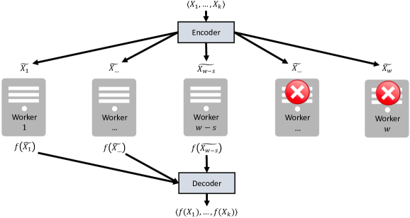
Figure 1: Overview of the coded computation model. A master uses $w$ workers to compute the value of the function $f$ at $k$ evaluation points subject to at most $s$ straggling workers.

We start by describing the coded computation model studied in this work which is based on the model considered in [31].

Setting: The setting is shown in Figure 1 and consists of one master and many workers. The master’s objective is to compute the value of a function $f$ at $k$ arbitrary input points $\langle X_{1},\ldots,X_{k}\rangle$ using the minimum necessary number $w$ of workers. Moreover, the function $f$ can be any function in a set of functions $\mathcal{F}$—henceforth denoted as a “function class”—and up to $s$ arbitrary workers may straggle (fail). To do so, the master “queries” each worker $i\in\{1,\ldots,w\}$ with the evaluation point $\widetilde{X_{i}}$, and the worker computes $f(\widetilde{X_{i}})$. At most $s$ arbitrary workers straggle and return nothing to the master; the remaining $w-s$ workers return their computed values to the master. The master must use the received subset of $\{f(\widetilde{X_{1}}),\ldots,f(\widetilde{X_{w}})\}$ to decode $\langle f(X_{1}),\ldots,f(X_{k})\rangle$ regardless of which worker outputs are missing. The threshold of the minimum number of workers which is sufficient to do so is defined as follows:

Definition 1 (Worker threshold).

The $(\mathcal{F},k,s)$-worker threshold is the minimum number $w_{\mathcal{F},k,s}$ of workers for which coded computation for any function $f$ in a function class $\mathcal{F}$ at any $k$ input points tolerating up to $s$ straggling workers is possible.

II-A Related Works

The domain of coded computation has received considerable attention in the recent past. We now briefly overview some of the relevant topics.

Most works have considered coded computation for functions within the domain of Cartesian products of multivariate polynomial functions. For example, many works have considered linear settings such as matrix-vector multiplication [3, 5, 6, 7, 4, 10, 11], convolution [8], linear transforms [9], etc. Several works have considered coded computation for bilinear matrix-matrix multiplication [12, 13, 14, 15, 16, 17, 18, 19, 20, 21, 22, 23], and, in [14], the authors designed a coded computation scheme to compute the matrix product of any number of matrices. In [31], the authors proposed a coded computation scheme for the Cartesian product of finitely many multivariate polynomial functions. Due to its generality, this scheme is portable; for example, it is is used in [32] for a setting involving multiple rounds of computation. Understanding coded computation for the large class of polynomial functions is a significant milestone in moving towards the ultimate goal of general functions.

Robust distributed computation for machine learning has received substantial interest. Most existing work focuses on the training phase, designing coded approaches for gradient computations during gradient descent. As the gradient is the summation of “partial gradients,” several works compute the partial gradients in a coded manner [33, 34, 35, 36, 37, 38]. Other works designed robust schemes to compute an approximate value of the gradient [39, 40, 41, 37, 42].

In [43], Kosaian et al. introduced coded computation for neural network inference. Providing resilience to inference tasks via coded computation requires supporting non-linear functions, as neural networks are highly non-linear. The authors propose a learning-based approach to overcome the challenge of non-linearity by using machine learning to learn an encoder and decoder for any given computation. Other works [44, 45] have further explored this learning-based approach for coded computation of inference tasks.

The learning-based approach approximately reconstructs unavailable function outputs. While approximation is suitable for ML inference tasks, it may not be suitable for others. Even ML tasks can benefit from exact reconstruction when it is achieved efficiently. This motivates pursuing mathematical constructs for coded computation for non-linear functions, as we do in this work.

II-B Coded Computation of Multivariate Polynomials

We now describe the coded computation setting studied in [31] in more detail, as it is closely related to the results presented in this work. This previously studied coded computation model is a special case of the setting described in the beginning of Section II with the following restrictions: (1) Coded computation is restricted to an arbitrary multivariate polynomial functions $f:\mathbb{V}\rightarrow\mathbb{U}$ for vector spaces $\mathbb{V}$ and $\mathbb{U}$ over a field $\mathbb{F}$. (2) The master queries each worker at an evaluation point which is a linear combination of the input points $\langle X_{1},\ldots,X_{k}\rangle$. Specifically, for each $i\in\{1,\ldots,w\}$, worker $i$ computes the value of $f(\cdot)$ at the evaluation point $\widetilde{X_{i}}=\sum_{j=1}^{k}\alpha_{i,j}X_{j}$ where $\alpha_{i,j}\in\mathbb{F}$. Moreover, the $\alpha_{i,j}$ are fixed apriori and are the same for any input points $\langle X_{1},\ldots,X_{k}\rangle$. (3) The master decodes $\langle f(X_{1}),\ldots,f(X_{k})\rangle$ using a linear combination of the received worker outputs. As the same linear encoding and decoding schemes are used for any $k$ input points, we denote this setting as input oblivious.

Lagrange Coded Computing (LCC) scheme [31]: The scheme computes the value of a multivariate polynomial function, $f:\mathbb{V}\rightarrow\mathbb{U}$, at input points $\langle X_{1},\ldots,X_{k}\rangle$ while tolerating up to $s$ straggling workers. When $deg(f)\leq(s+1)$, the LCC scheme computes the univariate polynomial $f(p(z))$, where $p(z)$ is a univariate polynomial of degree at most $k-1$ passing through the $k$ input points. Specifically, for $1\leq i\leq k$ and distinct $\beta_{1},\ldots,\beta_{k}\in\mathbb{F}$, $p(\beta_{i})=X_{i}$. The scheme computes $f(p(z))$ by using each of the $w=deg(f(p(z)))+s+1$ workers to compute the value of $f(p(z))$ at a distinct point. It then uses polynomial interpolation to recover $f(p(z))$ while tolerating any $s$ straggling workers. Finally, the scheme decodes each $f(X_{i})=f(p(\beta_{i}))$. When $(s+1)<deg(f)$, the LCC scheme uses $(s+1)$-wise replication with $w=k(s+1)$ workers and direct decoding. The authors prove a lower bound for this input oblivious setting, showing that any scheme requires at least $min(k(s+1),(k-1)deg(f)+s+1)$ workers.

III Locality-Based Model for Coded Computation

In this section, we propose a new locality-based model for coded computation; this model provides a unified viewpoint for coded computation and enables reduced worker threshold in the domain of multivariate polynomial computations compared to existing models.

III-A Comparison to Existing Model

The two key aspects of the locality-based model of coded computation considered in this work are: First, for any $k$ input points, the master may query each worker at an arbitrary evaluation point. Second, the decoding function can be an arbitrary function of the received worker outputs. This setting is a generalization of the model considered in [31]; in the model used in [31], the coded computation scheme is required to use the same linear encoding and decoding scheme for every $k$ input points and is therefore denoted as input oblivious. The flexibility to adapt to specific input points is fundamental to exploit locality properties of the input points, as we will see later.

In this setting, the computational complexity of the master (for encoding and decoding) can be higher than in the input oblivious setting, while the computational complexity of the workers remains the same in both settings. Given that there is only one master while there are numerous workers, we argue that the reduction in the number of workers needed justifies the increase in computational complexity of the master. In certain applications, the extra work of the master may be amortized over multiple rounds of coded computation. For example, in gradient descent for machine learning applications, the gradient is computed at the same points over multiple rounds. Thus, the master might identify locality properties of the input points (as will be described in Section V) in the first iteration and reuse these locality properties in later rounds at no additional cost.

III-B Preliminaries

We now provide a few relevant definitions from coding theory. In these definition and later in this work, $[i]$ denotes $\{1,\ldots,i\}$. Moreover, when considering the Cartesian product of multivariate polynomial functions $f(X)=(f_{1}(X),\ldots,f_{m}(X))$, the convention of $deg(f)=max_{i\in[m]}deg(f_{i})$ is used.

Definition 2 (Distance).

Codewords $c_{1}$ and $c_{2}$ of a code $C$ have distance $\Delta(c_{1},c_{2})$ of the number of symbols in which $c_{1}$ and $c_{2}$ differ.

Definition 3 (Hamming ball).

For a codeword $c$ of a code $C$, the Hamming ball $B(c,r)=\{c^{\prime}\in C\mid\Delta(c,c^{\prime})\leq r\}$.

Definition 4 (Punctured code).

For a code $C\subseteq\mathbb{U}^{n}$ and a subset $I=\{i_{1},\ldots,i_{l}\}\subseteq[n]$, the punctured code $C_{I}=\{c_{I}=(c_{i_{1}},\ldots,c_{i_{l}})\mid c=(c_{1},\ldots,c_{n})\in C\}$ is the code formed by restricting the codewords of $C$ to the symbols corresponding to $I$.

III-C Computational Locality

Under the coded computation setting, the objective is to design a scheme applicable to any function in a function class (such as multivariate polynomial functions). This motivates developing a suitable notion of locality for a function class, as we do in this section. In order to do so, we define a new notion of locality for an appropriately defined code associated with a function class and use this definition to define locality of a function class. We later show that the computational locality of a function class relates directly to its worker threshold under coded computation (i.e. computational locality is the analog of the number of workers needed for coded computation).

Throughout this section, let $\mathcal{F}$ be a class of functions between finite vector spaces $\mathbb{V}=\{v_{1},\ldots,v_{n}\}$ and $\mathbb{U}$ over a finite field $\mathbb{F}_{q}$ and $s$ be a positive integer.

To begin, a codeword is defined for any function.

Definition 5 (Associated codeword).

For a function $f$ over domain $\mathbb{V}$, the associated codeword is

$c^{f}=(f(v_{1}),\ldots,f(v_{n}))$.

Existing literature on locality of codes [25, 26, 27, 28, 29, 30] usually considers a code where each code symbol appears exactly once. The associated codeword reflects this convention. In contrast, the coded computation domain admits replicating a computation over multiple workers, motivating the need for the below definition.

Definition 6 (Repeated codeword).

For a codeword $c=(c_{1},\ldots,c_{n})\in\mathbb{U}^{n}$, the repeated codeword is

$c^{\langle s+1\rangle}=((c_{1},1),\ldots,(c_{n},1),\ldots,(c_{1},s+1),\ldots,(c_{n},s+1)).$

The repeated codeword $c^{\langle s+1\rangle}$ repeats the codeword $(s+1)$ times and appends to each repeated code symbol one label from $[s+1]$ for clarity of exposition.

Next, the above definitions are extended to apply to a function class. Specifically, Definition 7 is used to define a code associated to the function class.

Definition 7 (Associated code).

For a function class $\mathcal{F}$, the associated code is $C^{\mathcal{F}}=\{c^{f}\mid f\in\mathcal{F}\}$.

Definition 8 generalizes the notion of a repeated codeword to a code.

Definition 8 (Repeated code).

For a code $C$, the repeated code is $C^{\langle s+1\rangle}=\{c^{\langle s+1\rangle}\mid c\in C\}$.

The computational locality of code symbols is defined and then used to define the computational locality of a code. The definition of computational locality of a code will then be used to define the relevant notion of locality for a function class.

Definition 9 (Computational locality of code symbols).

Let $k\leq n$ and $s$ be non-negative integers and $I=\{i_{1},\ldots,i_{k}\}\subseteq[n]$. The computational locality $L_{I,s}$ of code symbols $C_{I}$ for code $C\subseteq\mathbb{U}^{n}$ is the minimum integer for which there exists a size $L_{I,s}$ set $J\subseteq[(s+1)n]$ such that $\forall c,c^{\prime}\in C^{\langle s+1\rangle},c_{J}^{\prime}\in B(c_{J},s)\Rightarrow c_{I}^{\prime}=c_{I}$.

At a high level, Definition 9 says that the code symbols $C_{I}$ can be uniquely decoded using any $L_{I,s}-s$ code symbols of a length $L_{I,s}$ punctured code of $C^{\langle s+1\rangle}$. Definition 9 naturally yields a definition for computational locality for a code itself.

Definition 10 (Computational locality of a code).

Let $k\leq n$ and $s$ be non-negative integers. The computational locality $L_{k,s}$ of a code $C\subseteq\mathbb{U}^{n}$ is $max_{I=\{i_{1},\ldots,i_{k}\}\subseteq[n]}(L_{I,s})$.

Finally, the computational locality of a function class is defined in terms of Definition 10.

Definition 11 (Computational locality of a function class).

Let $k\leq n$ and $s$ be non-negative integers. The function class $\mathcal{F}$ has computational locality $L_{k,s}(\mathcal{F})$ where $L_{k,s}(\mathcal{F})$ is the computational locality of the associated code $C^{\mathcal{F}}$.

Under Definition 11, for a function class $\mathcal{F}$ and any input code symbols, one may consider an arbitrary punctured code of the repeated code. The analog of this property under coded computation is that when designing coded computation schemes, for any specific $k$ input points one can query the workers at arbitrary evaluation points. This flexibility with queries directly results in a lower worker threshold under the locality-based model for coded computation than is possible in the input oblivious setting for multivariate polynomial functions.

III-D Connection Between Computational Locality and Coded Computation

Below, it is shown that the computational locality of a function class is equivalent to its worker threshold (i.e. the minimum necessary number of workers) under coded computation. The proof follows from the above definitions and is included for completeness.

Theorem 1 (Coded computation via computational locality).

Let $k\leq|\mathbb{V}|=n$ and $s$ be non-negative integers. The computational locality of the function class $\mathcal{F}$ equals the $(\mathcal{F},k,s)$-worker threshold (i.e. $L_{k,s}(\mathcal{F})=w_{\mathcal{F},k,s}$).

Proof:

Consider any input $\langle X_{1},\ldots,X_{k}\rangle$ and related size $k$ set $I\subseteq[n]$, where $c_{I}^{f}=\langle f(X_{1}),\ldots,f(X_{k})\rangle$. Every set $J\subseteq[(s+1)n]$ (of some size $j$) corresponds to $\langle\widetilde{X_{1}},\ldots,\widetilde{X_{j}}\rangle$ such that $\langle f(\widetilde{X_{1}}),\ldots,f(\widetilde{X_{j}})\rangle=(c^{f})^{\langle s+1\rangle}_{J}$. As each worker computes exactly one code symbol, the number of workers needed for coded computation equals the number of code symbols required to uniquely decode $c^{f}_{I}$ when missing up to $s$ worker outputs (respectively code symbols). This holds for any $k$ input points, hence the maximum over all input points.

∎

A simple upper bound on the computational locality of a function class follows from the $(s+1)$-wise repeating of code symbols.

Remark 1.

The computational locality $L_{k,s}(\mathcal{F})$ is at most $k(s+1)$.

IV Computational Locality of Multivariate Polynomials

In this section, we discuss how to adapt existing locality results into the coded computation setting. We demonstrate how to design coded computation schemes for degree bounded multivariate polynomials by using local recovery schemes for the associated Reed-Muller code. In so doing, we reproduce the best known coded computation scheme for multivariate polynomial functions [31].

The following notation is used in this section. Let function class $\mathcal{F}=\mathbb{F}_{q}[x_{1},\ldots,x_{m}]$ be the set of all multivariate polynomials of total degree at most $d$ for a finite field $\mathbb{F}_{q}=\{\alpha_{1},\ldots,\alpha_{q}\}$. Let $f\in\mathcal{F}$ and consider non-negative integers $k$ and $s$. By definition, the associated code $C^{\mathcal{F}}$ is a Reed-Muller code [46, 47].

Reed-Muller codes are well-studied and exhibit many useful algebraic properties. The most relevant such property to this work is that for any univariate polynomial $p:\mathbb{F}_{q}\rightarrow\mathbb{F}_{q}^{m}$, the corresponding vector $\left(f(p(\alpha_{1})),\ldots,f(p(\alpha_{q}))\right)$ is a puncturing of $c^{f}$. Moreover, the composition $f(p(z))$ is a degree $d^{\prime}=deg(f)deg(p)$ univariate polynomial. One can recover a degree $d^{\prime}$ univariate polynomial via polynomial interpolation of $d^{\prime}+1$ distinct points. Prior works in the literature on the locality of codes have exploited this property in designing local recovery schemes for Reed-Muller codes[48, 49, 50, 25, 51]. We next discuss such existing local recovery schemes for Reed-Muller codes and use them to prove a computational locality result for multivariate polynomial functions. At a high level, we show that every set of $k$ code symbols is part of a corresponding group of $(k-1)d+s+1$ code symbols for which every group of $s$ symbols is redundant. This requires the added restriction of a sufficiently large field size (i.e. $(k-1)d+s+1\leq q$), which we will assume henceforth.

Figure 2: Example of a local recovery scheme for the degree $2$ multivariate polynomial $f(z_{1},z_{2})=.5z_{1}z_{2}$ at $x=(2,1)$. The line $x+zv$ is considered for $z\in\mathbb{R}$ and $v=(4,2).$ The univariate polynomial $f(x+zv)$ is interpolated using $4$ distinct queries tolerating up to $1$ straggling query.

Variants of the following local recovery scheme for Reed-Muller codes were considered by several previous works [48, 49, 50, 25]. To recover the value of a polynomial $f$ at a point, $f(x)$, consider the affine line $P=\{x+zv\mid z\in\mathbb{F}_{q}\}$ for some $v\neq 0\in\mathbb{F}_{q}^{m}$. Let $h(z)=f(x+zv)$ be the degree at most $d$ univariate polynomial restriction of $f$ to $P$ with the property that $h(0)=f(x)$. One can interpolate $h(z)$ by querying it along any $d+s+1$ distinct evaluation points when at most $s$ queries straggle (i.e. are lost). A simple example of this scheme is demonstrated in Figure 2 for the specific polynomial $f(z_{1},z_{2})=.5z_{1}z_{2}$ for $z_{1},z_{2}\in\mathbb{R}$.

Another local recovery scheme follows a similar approach using using a degree $2$ curve instead of an affine line [51]. Consider the curve $P=\{x+zv_{1}+z^{2}v_{2}\mid z\in\mathbb{F}_{q}\}$ for $v_{1},v_{2}\neq 0\in\mathbb{F}_{q}^{m}$. Let $h(z)=f(x+zv_{1}+z^{2}v_{2})$ be the degree at most $2d$ univariate polynomial restriction of $f$ to $P$ such that $h(0)=f(x)$. Interpolation of $h(z)$ follows immediately from querying $h(z)$ at any $2d+s+1$ distinct evaluation points subject to at most $s$ straggling queries.

The above local recovery schemes were designed to recover the value of a polynomial $f$ at a single input point $x$. Yet the computational locality setting requires evaluating $f$ at multiple input points. A standard generalization of the above schemes using analogous technique with a parameterized degree $d^{\prime}$ curve is simple to convert to the computational locality regime. Under the generalized local recovery scheme, to recover $f(x)$, one can consider the degree $d^{\prime}$ curve $P=\{x+\sum_{j=1}^{d^{\prime}}z^{j}v_{j}\mid z\in\mathbb{F}_{q}\}$ for $v_{1},\ldots,v_{d^{\prime}-1},v_{d^{\prime}}\neq 0\in\mathbb{F}_{q}^{m}$. Let $h(z)=f(x+\sum_{j=1}^{d^{\prime}}z^{j}v_{j})$ be the degree at most $d^{\prime}d$ univariate polynomial restriction of $f$ to $P$ such that $h(0)=f(x)$. One can interpolate $h(z)$ by querying it along $d^{\prime}d+s+1$ distinct evaluation points tolerating up to $s$ straggling queries.

Figure 3: Example of a local recovery scheme for the degree $2$ multivariate polynomial $f(z_{1},z_{2})=.5z_{1}z_{2}$ at $\langle x_{1},x_{2},x_{3}\rangle=\langle(0,0),(2,1),(4,0)\rangle$. The degree $2$ curve $p(z)=(z,1-\frac{(z-2)(z-2)}{4})$ is considered for $z\in\mathbb{R}$. This curve intersects $x_{1}$ at $z=0$, $x_{2}$ at $z=2$, and $x_{3}$ at $z=4$. The univariate polynomial $f(p(z))$ is interpolated using any $5$ out of $6$ distinct queries.

One can adapt the above generalized local recovery scheme for Reed-Muller codes, via the locality-based model, into a result on the computational locality of $\mathcal{F}$. For any $k$ input points $\langle X_{1},\ldots,X_{k}\rangle$, there is a degree $d^{\prime}\leq k-1$ curve, $p(z)$, along with $\alpha_{1},\ldots,\alpha_{k}\in\mathbb{F}_{q}$, so that $p(\alpha_{i})=X_{i}$ for all $1\leq i\leq k$. Thus, the local recovery scheme corresponding to $P_{X_{1},\ldots,X_{k}}=\{p(z)\mid z\in\mathbb{F}_{q}\}$ computes $h(z)=f(p(z))$ subject to $s$ stragglers; furthermore, $\langle h(\alpha_{1}),\ldots,h(\alpha_{k})\rangle=\langle f(X_{1}),\ldots,f(X_{k})\rangle.$ A simple illustration of this scheme is shown in Figure 3 for the polynomial $f(z_{1},z_{2})=.5z_{1}z_{2}$ for $z_{1},z_{2}\in\mathbb{R}$. The aforementioned local recovery scheme demonstrates that $\mathcal{F}$ has computational locality $L_{k,s}(\mathcal{F})\leq(k-1)d+s+1$. Combining this bound with that of $(s+1)-$wise replication observed in Remark 1 leads to the following result.

Theorem 2.

The computational locality for total degree at most $d$ multivariate polynomials is $L_{k,s}(\mathcal{F})\leq min(k(s+1),(k-1)d+s+1)$.

Although the focus of this section was on multivariate polynomial functions in $\mathcal{F}$ from $\mathbb{F}_{q}^{m}$ to $\mathbb{F}_{q}$, the techniques used here easily extend, through component-wise application, to the setting of Cartesian products of functions in $\mathcal{F}$.

IV-A Computational Locality-Based Interpretation of Existing Work

The LCC scheme [31] computes the value of $f$, the Cartesian product of any multivariate polynomials, at $k$ points tolerating up to $s$ stragglers. The scheme either (1) replicates each computation over $(s+1)$ workers or (2) computes the univariate polynomial $f(p(z))$ where $p(z)$ is the Cartesian product of degree at most $k-1$ polynomials passing through the $k$ input points. This follows from applying component-wise polynomial interpolation to $(k-1)deg(f)+s+1$ distinct evaluation points of $f(p(z))$. Thus, the LCC scheme can be viewed as the analogue of the final Reed-Muller local recovery scheme described in Section IV (combined with $(s+1)-$wise replication).

IV-B Computational Locality with Corruptions

We next consider the notion of a “computational locality with corruptions” of a function class $\mathcal{F}$ over $k$ input points which incorporates up to $b$ corrupt in addition to $s$ straggling queries. Computational locality with corruptions is analogous to a coded computation setting containing up to $b$ byzantine (adversarial) as well as $s$ straggling servers.

When $\mathcal{F}$ is a class of total degree at most $d$ multivariate polynomial functions, it is simple to adapt the aforementioned local recovery schemes to apply to the new setting. For example, one can still compute the values of any $f\in\mathcal{F}$ at $k$ points by obtaining the univariate polynomial restriction of $f$ to $P$, where $P$ is a degree at most $k-1$ curve passing through all $k$ input points. To do so, one can use the Berlekamp-Welsh algorithm on $(k-1)d+2b+1$ received (non-straggling) points, rather than interpolating $(k-1)d+1$ received points with no corruptions [52]. Moreover, one can adapt the simple $(s+1)$-wise replication technique to such a setting by replicating each input instead $(s+2b+1)$ times and using majority-based decoding.

Theorem 3.

The function class $\mathcal{F}$ of total degree at most $d$ multivariate polynomials for $k$ input points, $b$ byzantine corruptions, and $s$ stragglers, has a worker threshold of at most $min(k(s+2b+1),(k-1)d+s+2b+1)$.

V Improved Worker Threshold via Locality

In Section IV, we have discussed the locality properties of multivariate polynomials at arbitrary input points without using the structure of the specific input points. The results from [31] show that the overhead in the number of workers is high for coded computation schemes which likewise are oblivious to the structure of the input points. Specifically, when tolerating up to $s$ stragglers for a polynomial of total degree at least $(s+1)$, it is impossible to outperform the factor $s$ overhead on the number of workers required by $(s+1)-$wise replication.

The focus of this section is how the locality-based approach to model coded computation aids in going beyond the worker threshold of the input oblivious setting. This improvement follows from enabling schemes to adaptively exploit the structure of specific input points. In Section V-A, we show how to leverage linear dependencies in the input points to reduce the required number of workers for coded computation of a homogeneous multivariate polynomial function. In Section V-B, we use homogenization—a technique by which one converts a multivariate polynomial into a homogeneous multivariate polynomial—to likewise exploit linear dependencies in the input points for non-homogeneous polynomial functions. This will establish that under the proposed locality-based model, the worker threshold is less than that of $(s+1)$-wise replication which is necessary in the input oblivious setting. Moreover, in Section V-C, we demonstrate concrete settings in which this improvement is significant. In Section V-D, we discuss the rich class of locality properties that coded computation schemes can exploit enabled by the proposed locality-based model. Finally, in Section V-E, we extend all of our results to a setting in which there are at most $b$ byzantine (adversarial) workers in addition to up to $s$ straggling workers.

V-A Coded Computation of Homogeneous Multivariate Polynomials

In this section, we focus on the class of homogeneous multivariate polynomial functions. Such polynomials have the fundamental property that multiplying the input by a field element is equivalent to multiplying the output by an associated power of the field element. We exploit this property in designing a novel coded computation scheme through leveraging locality (in the form of linear dependencies) of the input points.

A homogeneous polynomial $f\in\mathbb{F}[x_{1},\ldots,x_{m}]$ is defined as $f(X)=\sum_{i\in I}p_{i}(X)$ for some index set $I$ where for each $i\in I$, $p_{i}\in\mathbb{F}[x_{1},\ldots,x_{m}]$ is a monomial with $deg(p_{i})=deg(f)$. Consequently, for any homogeneous polynomial $f$ and any $\alpha\in F$, $f(\alpha X)=\alpha^{deg(f)}f(X).$

Figure 4: Example for locality-based coded computation of a homogeneous polynomial, $f$. Computing $f(l(z))$ determines the value of $f$ at all three input points due to homogeneity.

Thus, in order to compute the value of $f$ on any input points, it suffices to compute the value of $f$ at nonzero multiples of the input points. One can exploit this property to design coded computation schemes using fewer workers than is possible in the input oblivious setting for linearly dependent input points. We summarize how a coded computation scheme can do so, discuss a simple example of such a scheme, and finally present an explicit construction in full detail.

Consider any minimal linearly dependent set of $k$ vectors (i.e. a set of linearly dependent vectors for which no strict subset is linearly dependent). There is a $p(z)$ which is the Cartesian product of degree at most $k-2$ univariate polynomials passing through a nonzero multiple of each of the $k$ vectors. Moreover, $f(p(z))$ is the Cartesian product of degree at most $deg(f)(k-2)$ univariate polynomials and can be interpolated (component-wise) using any $deg(f)(k-2)+1$ distinct evaluations. Hence, a coded computation scheme can compute $f(p(z))$ and thereby obtain the values of $f$ at nonzero multiples of the $k$ input points. By homogeneity, this is sufficient to decode $f$ at the $k$ input points. In contrast, a polynomial $p^{\prime}(z)$ passing through the $k$ specific points can be of degree $k-1$; a similar scheme computing $f(p^{\prime}(z))$ would require $deg(f)(k-1)+1$ distinct evaluations of $f(p^{\prime}(z))$ to be received for interpolation.

In Figure 4, we discuss a simple example of a coded computation scheme for a homogeneous polynomial $f$ subject to $s$ straggling workers where $2\leq(s+1)=deg(f)$. The example contains three distinct linearly dependent input points in the x-y plane, $\langle(0,1),(2,0),(2,1)\rangle$. The line $l(z)$ intersects a nonzero multiple of each input, and by homogeneity, $f(2X)=2^{deg(f)}f(X)$ for $\alpha\in\mathbb{R}$. Hence, computing $f(l(z))$ is sufficient to determine $\langle f((0,1)),f((2,0)),f((2,1))\rangle$; this requires $2(s+1)$ workers, while the worker threshold in the input oblivious setting is $3(s+1).$

We now present the homogeneous scheme for any $k$ minimal linearly dependent input points. The scheme is systematic and uses linear encoding and decoding.

Input: $\langle X_{1},\ldots,X_{k}\rangle$ where $X_{j}\in\mathbb{F}^{m}$ for $1\leq j\leq k$ and $\sum_{i=1}^{k-1}\alpha_{i}X_{i}=X_{k}$ for $\alpha_{1},\ldots,\alpha_{k-1}\in\mathbb{F}\setminus\{0\}$ for a field $\mathbb{F}$. A positive integer $s$ of straggling workers and $deg(f),$ the degree of the polynomial to be computed.

Evaluation points: Let the first $k$ evaluation points be $\widetilde{X_{i}}=X_{i}$ for $1\leq i\leq k$. Let $\beta_{1},\ldots,\beta_{(k-2)deg(f)+s+1}\in F$ be distinct elements and $p^{*}(z)=\sum_{i=1}^{k-1}\alpha_{i}X_{i}.\prod_{j\in[k-1]\setminus\{i\}}(z-\beta_{j})(\beta_{k}-\beta_{j})^{-1}.$ Let the remaining evaluation points be $\widetilde{X_{i}}=p^{*}(\beta_{i})$ for $k+1\leq i\leq(k-2)deg(f)+s+1$. The scheme queries $f(\widetilde{X_{i}})$ for $1\leq i\leq(k-2)deg(f)+s+1$.

Decoding: For each received worker output $i\in[k-1]$ compute $f(p^{*}(\beta_{i}))=f(\widetilde{X_{i}})\cdot\left(\alpha_{i}\prod_{j\in[k-1]\setminus\{i\}}\frac{\beta_{i}-\beta_{j}}{\beta_{k}-\beta_{j}}\right)^{deg(f)}.$ As $f(\widetilde{X_{i}})=f(p^{*}(\beta_{i}))$ for $k\leq i\leq(k-2)deg(f)+s+1$, the scheme now has access to $(k-2)deg(f)+1$ distinct evaluations of $f(p^{*}(z))$. It uses them to interpolate $f(p^{*}(z))$. Decoding follows from setting $f(X_{k})=f(p^{*}(\beta_{k}))$ and for $i\in[k-1]$, setting $f(X_{i})=f(p^{*}(\beta_{i}))\cdot\left(\alpha_{i}\prod_{j\in[k-1]\setminus\{i\}}\frac{\beta_{i}-\beta_{j}}{\beta_{k}-\beta_{j}}\right)^{-deg(f)}.$

Correctness of the homogeneous scheme is shown in Theorem 4.

Theorem 4.

Let $\langle X_{1},\ldots,X_{k}\rangle$ be $k$ input points over $\mathbb{F}^{m}$ for field $\mathbb{F}$ such that $\sum_{i=1}^{k-1}\alpha_{i}X_{i}=X_{k}$ for $\alpha_{1},\ldots,\alpha_{k-1}\in\mathbb{F}\setminus\{0\}$. Let $s$ be a non-negative integer and $|\mathbb{F}|\geq(k-2)deg(f)+s+1$. Then the homogeneous scheme computes $\langle f(X_{1}),\ldots,f(X_{k})\rangle$ tolerating up to $s$ straggling workers using $(k-2)deg(f)+s+1$ workers.

Proof:

Let $\lambda_{i}=\alpha_{i}\prod_{j\in[k-1]\setminus\{i\}}(\beta_{i}-\beta_{j})(\beta_{k}-\beta_{j})^{-1}$ and note that $\lambda_{i}\in\mathbb{F}\setminus\{0\}$ for $1\leq i<k.$ Thus, $p^{*}(\beta_{k})=\sum_{i=1}^{k-1}\alpha_{i}X_{i}=X_{k}$ and for $1\leq i<k$ $p^{*}(\beta_{i})=X_{i}\lambda_{i}.$ Due to the homogeneity of $f$, this means $f(p^{*}(\beta_{i}))=\lambda_{i}^{deg(f)}f(X_{i})$ for $1\leq i<k$ and $f(p^{*}(\beta_{k}))=f(X_{k})$.

As $deg(p^{*}(z))\leq k-2$, one can interpolate $f(p^{*}(z))$ with any $(k-2)deg(f)+s+1$ distinct evaluations of $f(p^{*}(z))$, while tolerating up to $s$ stragglers. One can decode $\langle f(X_{1}),\ldots,f(X_{k})\rangle$ using $f(p^{*}(z)).$

∎

One can apply the homogeneous scheme to any $k>m$ input points over $\mathbb{F}^{m}$ by using Gaussian Elimination to partition the input points into $T_{1},\ldots,T_{t},$ and $E$. Each $T_{i}$ for $1\leq i\leq t$ is comprised of a set of minimal linearly dependent input points where $t\geq\lfloor\frac{k}{m+1}\rfloor$ and $E$ contains the at most $m$ remaining input points. One can apply the homogeneous scheme to each of $T_{1},\ldots,T_{t}$ and $(s+1)$-wise replication to each input point in $E$, provided the field size is at least $(m-1)deg(f)+s+1$. When $deg(f)=s+1$, this scheme combining homogeneous scheme with $(s+1)-$wise replication requires at most $(k-t)(s+1)$ workers. In contrast, the worker threshold under coded computation of the input oblivious setting is $k(s+1)$. This leads to the following result.

Theorem 5 (Improved worker threshold for homogeneous polynomials).

Let $\mathcal{F}$ be the function class a total degree $(s+1)$ homogeneous polynomial over domain $\mathbb{F}^{m}$. For $k$ input points where $(m+1)|k$ and at most $s$ stragglers, the worker threshold under coded computation in the locality-based model is at most $k\frac{m}{m+1}(s+1)$.

V-B Coded Computation of Non-Homogeneous Multivariate Polynomials

We have shown for homogeneous multivariate polynomial functions that the worker threshold under the locality-based model for coded computation is lower than that of the input oblivious setting. In this section, we extend this result to non-homogeneous multivariate polynomial functions by combining the homogeneous scheme and the technique of homogenizing polynomials.

We begin by reviewing homogenizing polynomials. Let $f\in\mathbb{F}[x_{1},\ldots,x_{m}]$ be a multivariate polynomial function for a field $\mathbb{F}$. The homogenizing polynomial of $f(x_{1},\ldots,x_{m})$ is defined as $f^{\prime}(r,(x_{1},\ldots,x_{m}))=r^{deg(f)}f(x_{1}r^{-1},\ldots,x_{m}r^{-1})$. Furthermore, $f^{\prime}$ is homogeneous and $f^{\prime}(1,(x_{1},\ldots,x_{m}))=f(x_{1},\ldots,x_{m})$. The point $(1,(x_{1},\ldots,x_{m}))$ is denoted as the “homogenizing” point of $(x_{1},\ldots,x_{m})$.

We now present the non-homogeneous scheme. The scheme works by converting the input points into homogenizing points and then applying the homogeneous scheme with the homogenizing polynomial $f^{\prime}$ using as input points the homogenizing points.

Input: $\langle X_{1},\ldots,X_{k}\rangle$ where each $X_{j}\in\mathbb{F}^{m}$ for $1\leq i\leq k$ and $\sum_{i=1}^{k-1}\alpha_{i}(1,X_{i})=(1,X_{k})$ for $\alpha_{1},\ldots,\alpha_{k-1}\in\mathbb{F}\setminus\{0\}$ for a field $\mathbb{F}$. A non-negative integer $s$ of straggling workers and $deg(f),$ the degree of the non-homogeneous polynomial.

Evaluation points: Identify the evaluation points $\widetilde{X_{i}}^{\prime}=(r_{i},X_{i}^{*})\in\mathbb{F}^{m+1}$ for $i\in[(k-2)deg(f)+s+1]$ used by the homogeneous scheme on the inputs of homogenizing points $\langle X_{1}^{\prime},\ldots,X_{k}^{\prime}\rangle=\langle(1,X_{1}),\ldots,(1,X_{k})\rangle,$ non-negative integer $s$, and $deg(f)$. Without loss of generality, do so with each $r_{i}\neq 0$. The scheme queries $f(\widetilde{X_{i}})=f(r_{i}^{-1}X_{i}^{*})$ for $i\in[(k-2)deg(f)+s+1]$.

Decoding: Multiply each received $f(\widetilde{X_{i}})=f(r_{i}^{-1}X_{i}^{*}),$ by $r_{i}^{deg(f)}$ to determine the value of $f^{\prime}$ at the corresponding evaluation points, namely $f^{\prime}(\widetilde{X_{i}^{\prime}})=f^{\prime}(r_{i},\widetilde{X_{i}})=r_{i}^{deg(f)}f(r_{i}^{-1}r_{i}^{-1}X_{i}^{*})$. Complete the homogeneous scheme decoding to determine $\langle f^{\prime}((1,X_{1})),\ldots,f^{\prime}((1,X_{k}))\rangle=\langle f(X_{1}),\ldots,f(X_{k})\rangle.$

Correctness of the non-homogeneous scheme is verified in Theorem 6.

Theorem 6.

Let $\langle X_{1},\ldots,X_{k}\rangle$ be $k$ input points over $\mathbb{F}^{m}$ for field $\mathbb{F}$ for which $\sum_{i=1}^{k-1}\alpha_{i}(1,X_{i})=(1,X_{k})$ for $\alpha_{1},\ldots,\alpha_{k-1}\in\mathbb{F}\setminus\{0\}$. Let $s$ be a non-negative integer and $|\mathbb{F}|\geq(k-2)(deg(f)+1)+s+1$. Then the non-homogeneous scheme computes $\langle f(X_{1}),\ldots,f(X_{k})\rangle$ tolerating up to $s$ straggling workers using $(k-2)deg(f)+s+1$ workers.

Proof:

Due to Theorem 4 and properties of homogenizing polynomials, we need only prove that there are enough distinct queries of each low degree curve so that each query of $f^{\prime}(\widetilde{X_{i}^{\prime}})=f^{\prime}(r_{i},X_{i}^{*})$ has $r_{i}\neq 0$ for $i\in[(k-2)deg(f)+s+1]$.

Recall from the proof of Theorem 4 that the evaluation points $\widetilde{X_{i}}$ for $i\in[(k-2)deg(f)+s+1]$ lie on the curve $p^{*}(z)$ (i.e. $\widetilde{X_{i}}=p^{*}(\beta_{i})$ for $\beta_{i}\in\mathbb{F}$). Moreover, for $i\in[k]$, the evaluation point $\widetilde{X_{i}}=p^{*}(\beta_{i})=(1,X_{i})$, the homogenizing point for the input point $X_{i}$. Therefore, the first coordinate of the output of $p^{*}(z)$ can only equal $0$ for at most $deg(p^{*}(z))$ inputs. Since $deg(p^{*}(z))\leq k-2$, the non-homogeneous scheme requires at most $(k-2)deg(f)+s+1$ evaluation points. Moreover, it discards at most $k-2$ points where $p^{*}(z)$ is $0$. This is feasible, as $|\mathbb{F}|\geq(k-2)(deg(f)+1)+s+1$. ∎

Similar to extending the homogeneous scheme to $k>m$ arbitrary input points in the homogeneous setting, one can extend the non-homogeneous scheme to apply to $k>m+1$ arbitrary input points over $\mathbb{F}^{m}$ in the non-homogeneous setting. To do so, one partitions the input points $\langle X_{1},\ldots,X_{k}\rangle$ into $T_{1},\ldots,T_{t},$ and $E$ using Gaussian Elimination. Each $T_{i}$ for $1\leq i\leq t$ consists of $e_{i}\leq m+2$ input points $\langle X^{(i)}_{1},\ldots,X^{(i)}_{e_{i}}\rangle$ such that the corresponding set of homogenizing points $\{(1,X^{(i)}_{1}),\ldots,(1,X^{(i)}_{e_{i}})\}$ is minimally linearly dependent. Moreover, $E$ contains the at most $m+1$ extra input points, and $t\geq\lfloor\frac{K}{m+2}\rfloor$. One can apply the non-homogeneous scheme to each of $T_{1},\ldots,T_{t}$ and $(s+1)$-wise replication to each input point in $E$, provided the field size is at least $m(deg(f)+1)+s+1$. Overall, this requires at most $(k-t)(s+1)$ workers when $deg(f)=(s+1)$. In contrast, the worker threshold in the input oblivious setting for coded computation is $k(s+1)$. This leads to the following result.

Theorem 7 (Improved worker threshold for non-homogeneous polynomials).

Let $\mathcal{F}$ be the function class a non-homogeneous multivariate polynomial of total degree $(s+1)$ over domain $\mathbb{F}^{m}$. For $k$ input points where $(m+2)|k$ and up to $s$ stragglers, the worker threshold under the locality-based model for coded computation is at most $k\frac{m+1}{m+2}(s+1)$.

While the improvement in worker threshold over that of input oblivious setting may not be substantial, Theorem 7 shows that the lower bound on worker threshold from [31] is not a fundamental barrier for coded computation of non-linear functions. This opens up the potential of more resource efficient coded computation schemes of non-linear functions.

V-C Sparse Linear Dependencies in Input Points

We have seen in Sections V-A and V-B coded computation schemes which exhibit improved worker threshold over the best possible in the input oblivious setting. The extent of the reduction in the number of workers needed depends on the sizes of minimal linearly dependent sets of input points. When the size of a set of linearly dependent vectors is small, we refer to it as “sparse” (i.e. involving few vectors). Under the locality-based model of coded computation, improvement in worker threshold is considerable when there are sparse linear dependencies in the input points. The fewer the number of input points per linear dependency, the more pronounced the improvement. In this section, we discuss how such sparse linear dependencies in the input points naturally arise in certain applications. We then consider the regime where the input points are over a finite vector space $\mathbb{V}=\mathbb{F}_{q}^{m}$ over a finite field $\mathbb{F}_{q}$. We show that if there are sufficiently many input points, then sparse linear dependencies in the input points must exist. This results in a significantly lower worker threshold under the locality-based approach for coded computation than the best possible in the input oblivious setting.

In certain applications, the set of input points is augmented with additional points. These extra points are each comprised of linear combinations of a small number of the original input points. For example, in one recently proposed approach to training neural networks for image classification [53], the authors propose “mixup”, wherein the training data is augmented with linear combinations of a small number of points from the original training data. For any two training data points, $X_{1}$ and $X_{2}$, a new training example $X_{1}\alpha+(1-\alpha)X_{2}$ for $0<\alpha<1$ might be added. Under the locality-based model for coded computation, one can exploit such sparse linear dependencies (involving the augmented data points) to reduce the required number of workers.

One can always exploit a set of minimal linearly dependent input points to reduce the worker threshold for homogeneous multivariate polynomial computations by using the homogeneous scheme. In contrast, for non-homogeneous multivariate polynomial computations, even for linearly dependent input points $\langle X_{1},\ldots,X_{k}\rangle$, the corresponding homogenizing points $\langle(1,X_{1}),\ldots,(1,X_{k})\rangle$ may be linearly independent. However, when a partition of the input points includes the disjoint linearly dependent sets $\{X_{1},\ldots,X_{k_{1}}\}$ and $\{X_{1}^{\prime},\ldots,X_{k_{2}}^{\prime}\}$, the set of homogenizing points $\{(1,X_{1}),\ldots,(1,X_{k_{1}}),(1,X_{1}^{\prime}),\ldots,(1,X_{k_{2}}^{\prime})\}$ is linearly dependent. This follows from the fact that either (1) at least one of $\{(1,X_{1}),\ldots,(1,X_{k_{1}})\}$ and $\{(1,X_{1}^{\prime}),\ldots,(1,X_{{k_{2}}}^{\prime})\}$ is linearly dependent or (2) $(1,0,\ldots,0)$ is in their intersection. Thus, it is always possible to exploit any two minimal linearly dependencies of disjoint input points to reduce the worker threshold by using the non-homogeneous scheme.

In Lemma 1, we show that whenever there are sufficiently many $(k)$ points, there exists a size $2e$ linearly dependent subset of these points. A finite vector space over a finite field $\mathbb{F}_{q}$ contains a fixed number of vectors, while the number of linear combinations with nonzero coefficients of $e$ out of $k$ input points is $(q-1)^{e}\binom{k}{e}.$ When $(q-1)^{e}\binom{k}{e}$ exceeds the size of the vector space, there exists $2$ distinct linear combinations of $e$ input points which are equal. The set of involved vectors in the $2$ linear combinations is therefore linearly dependent.

Lemma 1.

For $e\geq 2$, a set of $k>2eq^{\frac{m}{e}-1}$ nonzero vectors of $\mathbb{F}_{q}^{m}$ must contain a size at most $2e$ linearly dependent subset.

Proof:

Let there be $k$ points $X_{1},\ldots,X_{k}\in\mathbb{F}_{q}^{m}\setminus\{0\}^{m}$ and consider the $\binom{k}{e}$ sets of $e$ points. If any such set is not full rank, the proof is concluded. Otherwise, for each size $e$ set $I\subseteq[k]$ there are $(q-1)^{e}$ distinct vectors of the form $\sum_{i\in I}\alpha_{i,I}X_{i}$ where $\alpha_{i,I}\in\mathbb{F}\setminus\{0\}$. Overall, there are $\binom{k}{e}(q-1)^{e}$ such vectors. When $\binom{k}{e}(q-1)^{e}>q^{m}$, there exists two of these vectors which are equal. As $\binom{k}{e}(q-1)^{e}\geq\frac{k}{e}^{e}(q-1)^{e}\geq\frac{k}{2e}^{e}q^{e}>q^{m},$ this condition is met when $k>2eq^{\frac{m}{e}-1}$.

Let $\sum_{i\in I}\alpha_{i,I}X_{i}=\sum_{j\in J}\alpha_{j,J}X_{j}$ for $\alpha_{i,I},\alpha_{j,J}\in\mathbb{F}\setminus\{0\}$ and distinct $I,J\subseteq[k]$. Then $\sum_{i\in I\setminus J}\alpha_{i,I}X_{i}-\sum_{j\in J\setminus I}\alpha_{j,J}X_{j}+\sum_{l\in I\cap J}(\alpha_{l,I}-\alpha_{l,J})X_{l}=0$. Both $I\setminus J$ and $J\setminus I$ are nonempty with all nonzero corresponding coefficients $\alpha_{i,I}$ (for $i\in I\setminus J$) and $\alpha_{j,J}$ (for $j\in J\setminus I$). Hence, there is a linear dependence of at most $2e$ terms.

∎

When there sufficiently many input points, there must be sparse linear dependencies in the input points by Lemma 1. Consequently, one can partition all but negligibly many of the input points into size at most $2e$ linearly dependent sets. Thus, for a homogeneous or non-homogeneous multivariate polynomial $f$ of total degree $(s+1)$, $s$ stragglers, and $k$ input points, one can apply the homogeneous scheme or the non-homogeneous scheme to the size at most $2e$ linearly dependent sets. Combining this with $(s+1)-$wise replication for the remaining input points requires $\approx k\frac{2e-1}{2e}(s+1)$ workers in total. In contrast, the worker threshold in the input oblivious setting is $k(s+1)$.

Theorem 8.

Suppose $\mathcal{F}$ be the function class of total degree $(s+1)$ polynomials over domain $\mathbb{F}_{q}^{m}$, at most $s$ workers straggle, and $k>2eq^{\frac{m+1}{e}-1}$. The worker threshold under locality-based coded computation is at most $k\left(\frac{2e-1}{2e}(s+1)+(s+1)\frac{2eq^{\frac{m+1}{e}-1}}{k}\right)$.

V-D General Class of Locality-Based Coded Computation Schemes

Under the locality-based model, coded computation schemes can leverage the advantageous structural properties of the specific input points. We showed in Sections V-A and V-B one way to leverage locality properties of input points to design coded computation schemes using fewer workers than is possible in the input oblivious setting. We demonstrate the richness of the class of methods for using locality properties of the input points by presenting two more techniques to exploit locality properties of the input points in Section V-D1. In Section V-D2, we discuss how one can use locality properties of the output points (i.e. the image of the input points under the computed function) to reduce the number of workers for coded computation.

V-D1 More on Locality in Input Points

We now discuss two additional locality properties of input points: First, we consider the simple scenario where input points lie on a particularly low degree curve and observe that the points have a useful locality structure. Specifically, suppose there are $k$ input points $\langle X_{1},\ldots,X_{k}\rangle$ over $\mathbb{F}^{m}$ for a field $\mathbb{F}$ and a degree at most $(k-2)$ curve $p^{*}(z)$ such that $p^{*}(\beta_{i})=X_{i}$ where $\beta_{i}\in\mathbb{F}$ for $i\in[k]$. For any $f$ which is the Cartesian product of multivariate polynomial functions, the univariate polynomial $f(p^{*}(z))$ can be interpolated (component-wise) using any $deg(f)deg(p^{*}(z))+1\leq deg(f)(k-2)+1$ distinct evaluations. Thus, the value of $f$ at the $k$ inputs can be computed while tolerating up to $s$ stragglers using $deg(f)(k-2)+s+1$ workers each querying a distinct evaluation of $f(p^{*}(z))$.

Second, we demonstrate a locality property of input points for multivariate polynomials in the following scenario, which we denote “intersecting curves;” there are two low degree curves which pass through distinct input points and also intersect each other. We design a scheme to exploit this structure to achieve lower worker threshold than is possible in the input oblivious setting. At a high level, the scheme interpolates the two low degree curves. Computing one curve is sufficient to compute the intersection point, which can then be used in interpolating the another other curve. The intersection point is used to make do with $2$ fewer queries.

Figure 5: Example for locality-based coded computation of a polynomial $f$ at $4$ input points using two intersecting lines. The lines $l_{1}(z)$ and $l_{2}(z)$ pass through the $4$ input points and intersect at $z=1$. Using the identity $f(l_{1}(1))=f(l_{2}(1))$ reduces the number of workers by $2$.

We begin by using a simple example of intersecting curves in Figure 5 before describing the scheme in detail. In the example, the lines $l_{1}(z)=(z,1-z/2)$ and $l_{2}(z)=(z,z/2)$ pass through the input points $\{(0,1),(2,0)\}$ and $\{(0,0),(2,1)\}$ while intersecting at $l_{1}(1)=l_{2}(1)=(1,.5)$. After computing $f(l_{1}(z))$, the point $f(l_{1}(1))=f(l_{2}(1))$ can be recovered and used in computing $f(l_{2}(z))$ (and vice versa). Consequently, querying the workers with evaluation points of $f$ along the two lines and exploiting the intersection point reduces the number of workers needed.

We now present the intersecting input curves scheme for any degree $d$ polynomial subject to $s$ stragglers for input points which lie on two low-degree intersecting curves.

Input: Distinct $\langle X_{1},\ldots,X_{k},X_{1}^{\prime},\ldots,X_{k^{\prime}}^{\prime}\rangle$ over $\mathbb{F}^{m}$ for field $\mathbb{F}$ where the lowest degree curves passing through $\langle X_{1},\ldots,X_{k}\rangle$ and $\langle X_{1}^{\prime},\ldots,X_{k^{\prime}}\rangle$ intersect. A non-negative integer $s$ of stragglers and $deg(f)$, the degree of the polynomial to be computed.

Evaluation point: Let $p(z)$ and $p^{\prime}(z)$ be the degree less than $k$ and $k^{\prime}$ univariate polynomials such that: (1) $p(\alpha_{i})=X_{i}$ for $\alpha_{i}\in\mathbb{F}$ and $i\in[k]$. (2) $p^{\prime}(\beta_{i})=X_{i}^{\prime}$ for $\beta_{i}\in\mathbb{F}$ and $i\in[k^{\prime}]$. (3) $p(z_{*})=p^{\prime}(z_{*^{\prime}}^{\prime})$ for some $z_{*},z_{*^{\prime}}^{\prime}\in\mathbb{F}$. For $i\in[deg(f)\cdot deg(p(z))+s]$, let $\widetilde{X_{i}}=f(p(\alpha_{i}))$ for distinct $\alpha_{i}\in\mathbb{F}\setminus\{z_{*}\}.$ For $deg(f)\cdot deg(p(z))+s\leq i\leq deg(f)\cdot(deg(p(z))+deg(p^{\prime}(z)))+2s$, let $\widetilde{X_{i}}=f(p^{\prime}(\beta_{i}))$ for distinct $\beta_{i}\in\mathbb{F}\setminus\{z_{*^{\prime}}^{\prime}\}.$ Query the $i$th worker at $\widetilde{X_{i}}$ to compute $f(\widetilde{X_{i}})$ for $i\in[deg(f)\cdot(deg(p(z))+deg(p^{\prime}(z)))+2s].$

Decoding: use the received queries to interpolate at least one of $f(p(z))$ or $f(p^{\prime}(z))$ and thereby recover $f(p(z_{*}))=f(p^{\prime}(z_{*^{\prime}}^{\prime}))$. Use the decoded intersection point and received points to interpolate the second curve. Decoding follows from setting $\langle f(X_{1}),\ldots,f(X_{k}),f(X_{1}^{\prime}),\ldots,f(X_{k^{\prime}}^{\prime})\rangle=\langle f(p(\alpha_{1})),\ldots,f(p(\alpha_{k})),f(p(\beta_{1})),\ldots,f(p(\beta_{k^{\prime}}))\rangle.$

Remark 2.

Correctness for the intersecting input curves scheme immediately follows from univariate polynomial interpolation when $|\mathbb{F}|\geq d(max(k,k^{\prime})-1)+s+1$.

In Lemma 2, we show that if there are enough input points in a finite domain ensure, then there must exist (1) two intersecting lines passing through $4$ input points or (2) three input points which lie on a line. One can exploit either property to reduce the number of workers in the computation. The result follows from the fact that with enough input points, the number of points on the lines between input points exceeds the total number of points in a finite domain. Hence, there must be lines between input points which intersect, necessitating (1) or (2).

Lemma 2.

Suppose there are $k$ distinct input points $\langle X_{1},\ldots,X_{k}\rangle$ over a finite vector space $\mathbb{F}_{q}^{m}$ for $k>1$ and $q>3$. If $k>8q^{\frac{m-1}{2}}$, there exists three input points which lie on a line or there exists four input points which lie on two lines which intersect.

Proof:

Consider $l_{i,j}(z)=X_{i}+(X_{j}-X_{i})z$ for $1\leq i<j\leq k$. There are $\frac{k(k-1)}{2}$ such lines, each with $q-2$ points $l_{i,j}(z)$ for $z\in\mathbb{F}_{q}\setminus\{0,1\}$. There are $q^{m}$ points in the domain. When $\frac{k(k-1)(q-2)}{2}>q^{m}$, there exists $l_{i,j}(z)$ and $l_{i^{\prime},j^{\prime}}(z)$ which intersect outside of $\{X_{i},X_{j},X_{i^{\prime}},X_{j^{\prime}}\}$. If $i\in\{i^{\prime},j^{\prime}\}$ or $j\in\{i^{\prime},j^{\prime}\}$, the two lines intersect in two distinct points and are the same line, hence three input points lie one a single line. If not, $i,j,i^{\prime},$ and $j^{\prime}$ are distinct, concluding the proof. ∎

One can combine the intersecting input curves scheme and polynomial interpolation along lines passing through $3$ input points (as described in the first paragraph of this section) into the following coded computation scheme for multivariate polynomials. Let $f$ be a multivariate polynomial of total degree $(s+1)$, $s$ be the maximum number of stragglers, and $\langle X_{1},\ldots,X_{k}\rangle$ be the input points. The scheme partitions the input points $\langle X_{1},\ldots,X_{k}\rangle$ into $T_{1},\ldots,T_{t},T_{1}^{\prime},\ldots,T_{t^{\prime}}^{\prime},$ and $E$. Each of $T_{i}$ for $1\leq i\leq t$ consists of $4$ input points which lie on two intersecting lines, each of $T_{i}^{\prime}$ for $1\leq i\leq t^{\prime}$ consists of $3$ input points which lie on a single line $l_{i}(z)$, and $E$ contains the extra input points. For each $T_{i}$ for $1\leq i\leq t$, the scheme can apply the intersecting input curves scheme by querying each line with $2s+1$ workers outside the intersection point (and using the recovered intersection point in decoding). For each $T_{i}^{\prime}$ for $1\leq i\leq t^{\prime}$, the scheme can use $deg(f)+s+1$ workers to interpolate $f(l_{i}(z)),$ thereby computing the value of $f$ at the at least $3$ input points. Finally, the scheme can apply $(s+1)-$wise replication to the input points in $E$. When the number of input points is $k\gg q^{\frac{m-1}{2}}$, by Lemma 2, $E$ contains a negligible fraction of the input points. Thus, the scheme requires fewer workers than the worker threshold in the input oblivious setting of $k(s+1)$.

Remark 3.

Let $f$ be a polynomial with $deg(f)=s+1$, there be at most $s$ stragglers, and the number of input points be $k>8q^{\frac{m-1}{2}}$. Then the above scheme requires at most $k(s+\frac{1}{2}+(s+1)\frac{8q^{\frac{m-1}{2}}}{k})$ workers.

V-D2 Locality in Output Points

Under the locality-based model, one can exploit locality properties of the output points (i.e. the image of the input points under the computed function) in addition to locality properties of the input points to reduce the number of workers needed. We now demonstrate that restricting the class of multivariate polynomial functions to require additional structure can impose locality properties of the output points. Such a restriction is relevant to applications that inherently do so; for example, considering matrix products rather than arbitrary polynomials in distributed matrix multiplication. Below, we use a simple example to illustrate that locality properties of output points can be used to reduce the number of workers used in coded computation. In general, identifying such properties is highly dependent on the on the function being computed and outside the scope of this work.

Consider the function class $\mathcal{F}^{\prime}=\{h(g(\cdot)),h\in\mathcal{H},g\in\mathcal{G}\}$ where $\mathcal{G}$ is a set of non-injective multivariate polynomials of total degree $d_{\mathcal{G}}$ and $\mathcal{H}$ is a set of multivariate polynomials of total degree $d_{\mathcal{H}}.$ Let $d=d_{\mathcal{G}}d_{\mathcal{H}}$. One can exploit two input points whose images are equal under $g(\cdot)$ to use fewer queries in a coded computation scheme. Suppose that the input points $\langle X_{1},\ldots,X_{k}\rangle$ are linearly independent, the degree $k-2$ curve $p(z)$ passes through the first $(k-1)$ input points, and there exists $z_{*}$ such that $g(p(z_{*}))=g(X_{k})$ for all $g\in\mathcal{G}$. Then a scheme which computes $h(g(p(z)))$ for $h\in\mathcal{H}$ and $g\in\mathcal{G}$ by querying workers with evaluation points of $h(g(p(\cdot)))$ and using polynomial interpolation can also decode $h(g(p(z_{*})))=h(g(X_{k}))$. This reduces the number of workers by at least $d$ compared to the approach of considering a degree $k-1$ polynomial $p^{\prime}(z)$ passing through all $k$ input points and computing $h(g(p^{\prime}(z)))$.

V-E Coded Computation with Byzantine Workers

As in Section IV-B, we consider a “coded computation with corruptions” setting incorporating at most $b$ byzantine in addition to $s$ straggling workers. It is simple to modify all proposed coded computation schemes to apply the new domain.

The proposed coded computation schemes are modified as follows: (1) Query each curve at an additional $2b$ distinct locations and use the Berlekamp-Welsh algorithm rather than polynomial interpolation [52]. Choose the query points for the intersecting input curves scheme to all be different from the intersection point. (2) Replace the combination of $(s+1)-$wise replication and direct decoding with $(s+2b+1)-$wise replication and majority-based decoding. Note that the field size requirements for each scheme increases by at most $2b$ in each setting.

Theorem 9.

Consider the coded computation with corruptions setting in which there are at most $b$ byzantine workers and $s$ straggling workers. The modified versions of the homogeneous scheme and non-homogeneous scheme provide robustness to the unreliable workers using $2b$ more workers compared to the original schemes, while the intersecting input curves scheme does so using $4b$ extra workers. Replacing $(s+1)-$wise replication and direct decoding with $(s+2b+1)-$wise replication and majority-based decoding likewise ensures resiliency to the unreliable workers and requires an additional $2b$ workers per input point.

It is simple to extend the modified homogeneous scheme and non-homogeneous scheme to apply to $k>m$ and $k>m+1$ input points respectively over $\mathbb{F}^{m}$. Doing so follows the nearly identical steps as were used in Sections V-A and V-B to extend the homogeneous scheme and non-homogeneous scheme to apply to $k>m$ and $k>m+1$ points; the only exception is in replacing the homogeneous scheme, non-homogeneous scheme, and $(s+1)-$wise replication scheme with the above modified schemes. When the total degree of the polynomial is $(s+2b+1)$, number of workers used in this setting by the LCC (i.e. the existing scheme requiring the fewest number of workers) is $k(s+2b+1)$. In contrast, fewer workers are needed by the modified homogeneous scheme and non-homogeneous scheme, as is discussed below.

Remark 4.

Let function classes $\mathcal{F}$ and $\mathcal{F}^{\prime}$ respectively be the sets of homogeneous and non-homogeneous multivariate polynomials of total degree $s+2b+1$ over domain $\mathbb{F}^{m}$. For $k$ and $k^{\prime}$ input points where $(m+1)|k$ and $(m+2)|k^{\prime}$, up to $s$ stragglers, and at most $b$ byzantine workers, the worker threshold under the locality-based model for coded computation is less than or equal to $k\frac{m}{m+1}(s+2b+1)$ and $k^{\prime}\frac{m+1}{m+2}(s+2b+1)$ respectively.

VI Locality-Based Interpretation of Matrix Multiplication Schemes

So far, we have considered a model of computation in which the objective is to evaluate a function $f$ over multiple input points $\langle X_{1},\ldots,X_{k}\rangle$. Coded computation can also be used for matrix multiplication of a single pair of large matrices [12, 13, 14, 16, 17, 18, 20, 23]. For simplicity of exposition, consider multiplying two square $(te\times te)$ matrices $A$ and $B$ with entries from a finite field $\mathbb{F}_{q}$, for some positive integers $t$ and $e$. In many applications, the overall matrix product is too large for a single worker to compute, but the matrix product subdivides into small modular pieces which can be distributed over several workers. One key distinction of this setting is that the process for dividing the computation into smaller components is not prescribed; indeed, the choice of what function(s) the workers compute can impose useful properties for the computation. Nonetheless, existing coded computation schemes for matrix multiplication can be viewed under the locality-based model proposed in this work.

We now consider two examples of schemes which compute the product of two matrices: the “polynomial code” [13] and the “MatDot” code [14]. Both schemes subdivide the input matrices by rows and columns and then use workers to compute the matrix-matrix products of the (smaller) coded matrices. The subdivision of the matrices combined with the matrix-matrix products computed by the workers induce computational locality properties which the schemes then exploit to perform the coded computation.

First, the polynomial code subdivides the computation into the matrix product of the rows of $A$ with the columns of $B$. Thus, $AB$ equals

$$\begin{bmatrix}A_{1}\\ \vdots\\ A_{t}\\ \end{bmatrix}\begin{bmatrix}B_{1}&\cdots&B_{t}\\ \end{bmatrix}=\begin{bmatrix}A_{1}B_{1}&\cdots&A_{1}B_{t}\\ \vdots&\ddots&\vdots\\ A_{t}B_{1}&\cdots&A_{t}B_{t}\\ \end{bmatrix}.$$

The workers each compute $f_{1}(\widetilde{A},\widetilde{B})=\widetilde{A}\widetilde{B}$ for $(e\times te)$ matrix $\widetilde{A}$ and $(te\times e)$ matrix $\widetilde{B}$. At a high level, the scheme computes each $A_{i}B_{j}$ for $1\leq i,j\leq t$, thereby determining $AB$. To do so while tolerating up to $s$ stragglers, the scheme considers the polynomials $p^{A}_{1}(z)=\sum_{i=1}^{t}A_{i}z^{i-1},$ $p^{B}_{1}(z)=\sum_{j=1}^{t}B_{j}z^{(j-1)t},$ and $p_{1}(z)=(p^{A}_{1}(z),p^{B}_{1}(z))$. The univariate polynomial $f_{1}(p_{1}(z))=\sum_{i=1}^{t}\sum_{j=1}^{t}A_{i}B_{j}z^{i-1+(j-1)t}$ has each of $A_{i}B_{j}$ for $1\leq i,j\leq t$ as the coefficient for a unique power of $z$. Thus, computing $f_{1}(p_{1}(z))$ is sufficient to compute $AB$. The polynomial code computes $f_{1}(p_{1}(z))$ using polynomial interpolation via $t^{2}+s$ workers each evaluating $f_{1}(p_{1}(z))$ at a unique evaluation point.

Second, the MatDot code divides the computation into the matrix product of the columns of $A$ with the rows of $B$. Thus, $AB$ equals

$$\begin{bmatrix}A_{1}&\cdots&A_{t}\\ \end{bmatrix}\begin{bmatrix}B_{1}\\ \vdots\\ B_{t}\\ \end{bmatrix}=\sum_{i=1}^{t}A_{i}B_{i}.$$

The workers each compute $f_{2}(\widetilde{A},\widetilde{B})=\widetilde{A}\widetilde{B}$ for $(te\times e)$ matrix $\widetilde{A}$ and $(e\times te)$ matrix $\widetilde{B}$. At a high level, the scheme computes the polynomial $\left(\sum_{i=1}^{t}A_{i}z^{i-1}\right)\left(\sum_{j=1}^{t}B_{j}z^{t-j}\right)$ and decodes the coefficient of $z^{t-1}$ as $AB=\sum_{i=1}^{t}A_{i}B_{i}$. Specifically, the scheme considers the polynomials $p^{A}_{2}(z)=\sum_{i=1}^{t}A_{i}z^{i-1}$, $p^{B}_{2}(z)=\sum_{j=1}^{t}B_{j}z^{t-j},$ and $p_{2}(z)=(p^{A}_{2}(z),p^{B}_{2}(z))$. It then interpolates $f_{2}(p_{2}(z))$ while tolerating up to $s$ stragglers by using $deg(f_{2}(p_{2}(z))=2t-1+s$ workers each evaluating $f_{2}(p_{2}(z))$ at a unique point. Finally, $AB$ is decoded as the coefficient of $z^{t-1}$ of $f_{2}(p_{2}(z)).$

Under the locality-based model, the polynomial and MatDot codes restricts their attention to the function classes $\mathcal{F}_{1}$ and $\mathcal{F}_{2}$ of multivariate polynomial functions corresponding to matrix-matrix multiplication of $(e\times te)$ and $(te\times e)$ matrices and respectively $(te\times e)$ and $(e\times te)$ matrices. Recall the notation from Definition 7 that $C^{\mathcal{F}_{1}}$ and $C^{\mathcal{F}_{2}}$ are the associated codes to these function classes; each function in $\mathcal{F}_{1}$ (respectively $\mathcal{F}_{2}$) corresponds to a codeword in $C^{\mathcal{F}_{1}}$ (respectively $C^{\mathcal{F}_{2}}$) which is a vector of all evaluations of the function. Consider the curves $P_{1}=\{(p^{A}_{1}(z),p^{B}_{1}(z))\mid z\in\mathbb{F}_{q}\}$ and $P_{2}=\{(p^{A}_{2}(z),p^{B}_{2}(z))\mid z\in\mathbb{F}_{q}\}.$ For any $k$ points of $P_{1}$, there is a is a size $k$ set $I_{1}$ such that the punctured code $C^{\mathcal{F}_{1}}_{I_{1}}$ corresponds to the $k$ points of $P_{1}$. Similarly, for any $k$ points of $P_{2}$, there is such a size $k$ corresponding set $I_{2}$ and punctured code $C^{\mathcal{F}_{2}}{I_{2}}$. The code symbols $C^{\mathcal{F}_{1}}_{I_{1}}$ have computational locality $L_{I_{1},s}\leq t^{2}+s$. This follows from the fact that for all $f_{1}\in\mathcal{F}_{1}$, $deg(f_{1}(p_{1}(z))=t^{2}-1$—which is strictly less than $deg(f_{1})deg(p_{1}(z))=2t(t-1)$. The polynomial code is designed to exploit this property. Specifically, it can be viewed as computing the function $f_{1}$ at the input points $\langle p_{1}(\alpha_{i})\mid 1\leq i\leq t^{2}\rangle$ using $t^{2}+s$ workers. Moreover, the computational locality of the code symbols $C^{\mathcal{F}_{2}}_{I_{2}}$ is $L_{I_{2},s}\leq 2t-1+s$. This holds since for all $f_{2}\in\mathcal{F}_{2}$, $deg(f_{2}(p_{2}(z))=2t-2$. The MatDot code leverages this fact to compute $f_{2}(p_{2}(z))$ using interpolation with $2t-1+s$ workers while tolerating up to $s$ stragglers. Finally, note that the different choice of subdivision of the matrices by the polynomial code and the MatDot code (leading to different function classes $\mathcal{F}_{1}$ and $\mathcal{F}_{2}$) results in different communication cost in addition to different computational locality properties. The function class $\mathcal{F}_{2}$ has a smaller computational locality than that of $\mathcal{F}_{1}$ at a higher communication cost.

In both of the above discussed works [13, 14], the setting of matrix-matrix multiplication of a single pair of large matrices $(A,B)$ using workers capable of only computing smaller (less computationally intensive) matrix-matrix products is considered. This setting naturally extends to the regime of computing the matrix products of multiple pairs of matrices $\langle(A_{i},B_{i})\mid i\in[k]\rangle$ using workers with similar computational restrictions, as has been studied in [22, 23]. Similar to above, the technique used in this domain is to first divide the matrices in a coded manner and than have the workers compute matrix products of the (smaller) coded matrices. This approach can likewise be interpreted under the locality-based model as a statement on the computational locality of the code symbols related to the matrix partitions.

VII Conclusion

In this work, we introduced a locality-based approach to model coded computation. This model enables the design of coded computation schemes which exploit the well-studied domain of local recovery of codes to reduce the required number of workers. We demonstrated that the proposed locality-based model for coded computation admits a lower worker threshold for multivariate polynomials than is possible under the existing input oblivious approaches. This establishes that a factor $s$ overhead in the number of servers—as in existing approaches—is not a fundamental requirement for robustness to $s$ stragglers for non-linear functions. The results presented, thus, signal the prospect of future resource efficient coded computation schemes for non-linear functions.

References

- [1] J. Dean and L. A. Barroso, “The tail at scale,” Communications of the ACM, vol. 56, no. 2, pp. 74–80, Feb. 2013. [Online]. Available: https://doi.org/10.1145/2408776.2408794
- [2] H. Weatherspoon and J. D. Kubiatowicz, “Erasure coding vs. replication: A quantitative comparison,” in Peer-to-Peer Systems, P. Druschel, F. Kaashoek, and A. Rowstron, Eds. Berlin, Heidelberg: Springer Berlin Heidelberg, 2002, pp. 328–337.
- [3] K. Lee, M. Lam, R. Pedarsani, D. Papailiopoulos, and K. Ramchandran, “Speeding up distributed machine learning using codes,” IEEE Transactions on Information Theory, vol. 64, no. 3, pp. 1514–1529, March 2018.
- [4] S. Li, M. A. Maddah-Ali, and A. S. Avestimehr, “A unified coding framework for distributed computing with straggling servers,” in 2016 IEEE Globecom Workshops (GC Wkshps), Dec 2016, pp. 1–6.
- [5] A. Reisizadeh, S. Prakash, R. Pedarsani, and A. S. Avestimehr, “Coded computation over heterogeneous clusters,” IEEE Transactions on Information Theory, vol. 65, no. 7, pp. 4227–4242, July 2019.
- [6] A. Mallick, M. Chaudhari, U. Sheth, G. Palanikumar, and G. Joshi, “Rateless codes for near-perfect load balancing in distributed matrix-vector multiplication,” Proc. ACM Meas. Anal. Comput. Syst., vol. 3, no. 3, Dec. 2019. [Online]. Available: https://doi.org/10.1145/3366706
- [7] Z. Lin, K. G. Narra, M. Yu, S. Avestimehr, and M. Annavaram, “Train where the data is: A case for bandwidth efficient coded training,” arXiv preprint arXiv:1910.10283, 2019.
- [8] S. Dutta, V. Cadambe, and P. Grover, “Coded convolution for parallel and distributed computing within a deadline,” in 2017 IEEE International Symposium on Information Theory (ISIT), June 2017, pp. 2403–2407.
- [9] S. Dutta, V. Cadambe, and P. Grover, “Short-dot: Computing large linear transforms distributedly using coded short dot products,” in Advances in Neural Information Processing Systems 29, D. D. Lee, M. Sugiyama, U. V. Luxburg, I. Guyon, and R. Garnett, Eds. Curran Associates, Inc., 2016, pp. 2100–2108. [Online]. Available: http://papers.nips.cc/paper/6329-short-dot-computing-large-linear-transforms-distributedly-using-coded-short-dot-products.pdf
- [10] N. Ferdinand and S. C. Draper, “Hierarchical coded computation,” in 2018 IEEE International Symposium on Information Theory (ISIT), June 2018, pp. 1620–1624.
- [11] S. Dutta, Z. Bai, H. Jeong, T. M. Low, and P. Grover, “A unified coded deep neural network training strategy based on generalized polydot codes,” in 2018 IEEE International Symposium on Information Theory (ISIT), June 2018, pp. 1585–1589.
- [12] K. Lee, C. Suh, and K. Ramchandran, “High-dimensional coded matrix multiplication,” in 2017 IEEE International Symposium on Information Theory (ISIT), June 2017, pp. 2418–2422.
- [13] Q. Yu, M. Maddah-Ali, and S. Avestimehr, “Polynomial codes: an optimal design for high-dimensional coded matrix multiplication,” in Advances in Neural Information Processing Systems 30, I. Guyon, U. V. Luxburg, S. Bengio, H. Wallach, R. Fergus, S. Vishwanathan, and R. Garnett, Eds. Curran Associates, Inc., 2017, pp. 4403–4413. [Online]. Available: http://papers.nips.cc/paper/7027-polynomial-codes-an-optimal-design-for-high-dimensional-coded-matrix-multiplication.pdf
- [14] S. Dutta, M. Fahim, F. Haddadpour, H. Jeong, V. Cadambe, and P. Grover, “On the optimal recovery threshold of coded matrix multiplication,” IEEE Transactions on Information Theory, vol. 66, no. 1, pp. 278–301, Jan 2020.
- [15] S. Wang, J. Liu, and N. Shroff, “Coded sparse matrix multiplication,” in Proceedings of the 35th International Conference on Machine Learning, ser. Proceedings of Machine Learning Research, J. Dy and A. Krause, Eds., vol. 80. Stockholmsmässan, Stockholm Sweden: PMLR, 10–15 Jul 2018, pp. 5152–5160. [Online]. Available: http://proceedings.mlr.press/v80/wang18e.html
- [16] T. Baharav, K. Lee, O. Ocal, and K. Ramchandran, “Straggler-proofing massive-scale distributed matrix multiplication with d-dimensional product codes,” in 2018 IEEE International Symposium on Information Theory (ISIT), June 2018, pp. 1993–1997.
- [17] S. Kiani, N. Ferdinand, and S. C. Draper, “Exploitation of stragglers in coded computation,” in 2018 IEEE International Symposium on Information Theory (ISIT), June 2018, pp. 1988–1992.
- [18] H. Jeong, F. Ye, and P. Grover, “Locally recoverable coded matrix multiplication,” in 2018 56th Annual Allerton Conference on Communication, Control, and Computing (Allerton), Oct 2018, pp. 715–722.
- [19] K. G. Narra, Z. Lin, M. Kiamari, S. Avestimehr, and M. Annavaram, “Slack squeeze coded computing for adaptive straggler mitigation,” in Proceedings of the International Conference for High Performance Computing, Networking, Storage and Analysis, ser. SC ’19. New York, NY, USA: Association for Computing Machinery, 2019. [Online]. Available: https://doi.org/10.1145/3295500.3356170
- [20] Q. Yu, M. Ali, and A. S. Avestimehr, “Straggler mitigation in distributed matrix multiplication: Fundamental limits and optimal coding,” IEEE Transactions on Information Theory, pp. 1–1, 2020.
- [21] H. Park, K. Lee, J. Sohn, C. Suh, and J. Moon, “Hierarchical coding for distributed computing,” in 2018 IEEE International Symposium on Information Theory (ISIT), June 2018, pp. 1630–1634.
- [22] Z. Jia and S. A. Jafar, “Cross subspace alignment codes for coded distributed batch computation,” 2019.
- [23] Q. Yu and A. S. Avestimehr, “Entangled polynomial codes for secure, private, and batch distributed matrix multiplication: Breaking the ”cubic” barrier,” 2020.
- [24] Q. Yu, N. Raviv, J. So, and A. S. Avestimehr, “Lagrange coded computing: Optimal design for resiliency, security and privacy,” arXiv preprint arXiv:1806.00939, 2018.
- [25] S. Yekhanin, “Locally decodable codes,” Foundations and Trends®in Theoretical Computer Science, vol. 6, no. 3, pp. 139–255, October 2012. [Online]. Available: http://dx.doi.org/10.1561/0400000030
- [26] P. Gopalan, C. Huang, H. Simitci, and S. Yekhanin, “On the locality of codeword symbols,” IEEE Transactions on Information Theory, vol. 58, no. 11, pp. 6925–6934, Nov 2012.
- [27] D. S. Papailiopoulos and A. G. Dimakis, “Locally repairable codes,” IEEE Transactions on Information Theory, vol. 60, no. 10, pp. 5843–5855, Oct 2014.
- [28] I. Tamo and A. Barg, “A family of optimal locally recoverable codes,” IEEE Transactions on Information Theory, vol. 60, no. 8, pp. 4661–4676, 2014.
- [29] N. Prakash, V. Lalitha, S. B. Balaji, and P. Vijay Kumar, “Codes with locality for two erasures,” IEEE Transactions on Information Theory, vol. 65, no. 12, pp. 7771–7789, Dec 2019.
- [30] P. Ramakrishnan and M. Wootters, “On taking advantage of multiple requests in error correcting codes,” in 2018 IEEE International Symposium on Information Theory (ISIT), June 2018, pp. 1340–1344.
- [31] Q. Yu, S. Li, N. Raviv, S. M. Mousavi Kalan, M. Soltanolkotabi, and S. Avestimehr, “Lagrange coded computing: Optimal design for resiliency, security, and privacy,” International Conference on Artificial Intelligence and Statistics (AISTATS 2019), Jan 2019. [Online]. Available: http://par.nsf.gov/biblio/10098884
- [32] C.-S. Yang, R. Pedarsani, and A. S. Avestimehr, “Timely-throughput optimal coded computing over cloud networks,” in Proceedings of the Twentieth ACM International Symposium on Mobile Ad Hoc Networking and Computing, ser. Mobihoc ’19. New York, NY, USA: Association for Computing Machinery, 2019, p. 301–310. [Online]. Available: https://doi.org/10.1145/3323679.3326528
- [33] R. Tandon, Q. Lei, A. G. Dimakis, and N. Karampatziakis, “Gradient coding: Avoiding stragglers in distributed learning,” in Proceedings of the 34th International Conference on Machine Learning, ser. Proceedings of Machine Learning Research, D. Precup and Y. W. Teh, Eds., vol. 70. International Convention Centre, Sydney, Australia: PMLR, 06–11 Aug 2017, pp. 3368–3376. [Online]. Available: http://proceedings.mlr.press/v70/tandon17a.html
- [34] W. Halbawi, N. Azizan, F. Salehi, and B. Hassibi, “Improving distributed gradient descent using reed-solomon codes,” in 2018 IEEE International Symposium on Information Theory (ISIT), June 2018, pp. 2027–2031.
- [35] S. Li, S. M. M. Kalan, A. S. Avestimehr, and M. Soltanolkotabi, “Near-optimal straggler mitigation for distributed gradient methods,” in 2018 IEEE International Parallel and Distributed Processing Symposium Workshops (IPDPSW). IEEE, 2018, pp. 857–866.
- [36] L. Chen, H. Wang, Z. Charles, and D. Papailiopoulos, “DRACO: Byzantine-resilient distributed training via redundant gradients,” in Proceedings of the 35th International Conference on Machine Learning, ser. Proceedings of Machine Learning Research, J. Dy and A. Krause, Eds., vol. 80. Stockholmsmässan, Stockholm Sweden: PMLR, 10–15 Jul 2018, pp. 903–912. [Online]. Available: http://proceedings.mlr.press/v80/chen18l.html
- [37] Z. Charles and D. Papailiopoulos, “Gradient coding using the stochastic block model,” in 2018 IEEE International Symposium on Information Theory (ISIT), June 2018, pp. 1998–2002.
- [38] M. Ye and E. Abbe, “Communication-computation efficient gradient coding,” in Proceedings of the 35th International Conference on Machine Learning, ser. Proceedings of Machine Learning Research, J. Dy and A. Krause, Eds., vol. 80. Stockholmsmässan, Stockholm Sweden: PMLR, 10–15 Jul 2018, pp. 5610–5619. [Online]. Available: http://proceedings.mlr.press/v80/ye18a.html
- [39] N. Raviv, R. Tandon, A. Dimakis, and I. Tamo, “Gradient coding from cyclic MDS codes and expander graphs,” in Proceedings of the 35th International Conference on Machine Learning, ser. Proceedings of Machine Learning Research, J. Dy and A. Krause, Eds., vol. 80. Stockholmsmässan, Stockholm Sweden: PMLR, 10–15 Jul 2018, pp. 4305–4313. [Online]. Available: http://proceedings.mlr.press/v80/raviv18a.html
- [40] H. Wang, Z. Charles, and D. Papailiopoulos, “Erasurehead: Distributed gradient descent without delays using approximate gradient coding,” arXiv preprint arXiv:1901.09671, 2019.
- [41] Z. Charles, D. Papailiopoulos, and J. Ellenberg, “Approximate gradient coding via sparse random graphs,” arXiv preprint arXiv:1711.06771, 2017.
- [42] C. Karakus, Y. Sun, S. Diggavi, and W. Yin, “Straggler mitigation in distributed optimization through data encoding,” in Advances in Neural Information Processing Systems 30, I. Guyon, U. V. Luxburg, S. Bengio, H. Wallach, R. Fergus, S. Vishwanathan, and R. Garnett, Eds. Curran Associates, Inc., 2017, pp. 5434–5442. [Online]. Available: http://papers.nips.cc/paper/7127-straggler-mitigation-in-distributed-optimization-through-data-encoding.pdf
- [43] J. Kosaian, K. Rashmi, and S. Venkataraman, “Learning a code: Machine learning for approximate non-linear coded computation,” arXiv preprint arXiv:1806.01259, 2018.
- [44] J. Kosaian, K. V. Rashmi, and S. Venkataraman, “Parity models: Erasure-coded resilience for prediction serving systems,” in Proceedings of the 27th ACM Symposium on Operating Systems Principles, ser. SOSP ’19. New York, NY, USA: Association for Computing Machinery, 2019, p. 30–46. [Online]. Available: https://doi.org/10.1145/3341301.3359654
- [45] K. G. Narra, Z. Lin, G. Ananthanarayanan, S. Avestimehr, and M. Annavaram, “Collage Inference: Tolerating Stragglers in Distributed Neural Network Inference using Coding,” arXiv preprint arXiv:1904.12222, 2019.
- [46] D. E. Muller, “Application of boolean algebra to switching circuit design and to error detection,” Transactions of the I.R.E. Professional Group on Electronic Computers, vol. EC-3, no. 3, pp. 6–12, Sep. 1954.
- [47] I. Reed, “A class of multiple-error-correcting codes and the decoding scheme,” Transactions of the IRE Professional Group on Information Theory, vol. 4, no. 4, pp. 38–49, 1954.
- [48] R. J. Lipton, “Efficient checking of computations,” in STACS 90, C. Choffrut and T. Lengauer, Eds. Berlin, Heidelberg: Springer Berlin Heidelberg, 1990, pp. 207–215.
- [49] D. Beaver and J. Feigenbaum, “Hiding instances in multioracle queries,” in STACS 90, C. Choffrut and T. Lengauer, Eds. Berlin, Heidelberg: Springer Berlin Heidelberg, 1990, pp. 37–48.
- [50] P. Gemmell, R. Lipton, R. Rubinfeld, M. Sudan, and A. Wigderson, “Self-testing/correcting for polynomials and for approximate functions,” in Proceedings of the Twenty-Third Annual ACM Symposium on Theory of Computing, ser. STOC ’91. New York, NY, USA: Association for Computing Machinery, 1991, p. 33–42. [Online]. Available: https://doi.org/10.1145/103418.103429
- [51] P. Gemmell and M. Sudan, “Highly resilient correctors for polynomials,” Information Processing Letters, vol. 43, no. 4, pp. 169 – 174, 1992. [Online]. Available: http://www.sciencedirect.com/science/article/pii/0020019092901952
- [52] L. R. Welch and E. R. Berlekamp, “Error correction for algebraic block codes,” Dec. 30 1986, uS Patent 4,633,470.
- [53] H. Zhang, M. Cisse, Y. N. Dauphin, and D. Lopez-Paz, “mixup: Beyond empirical risk minimization,” arXiv preprint arXiv:1710.09412, 2017.