Optimal Competitive Ratio for Reusable Resource Allocation Goyal, Iyengar, Udwani Asymptotically Optimal Competitive Ratio for Online Allocation of Reusable Resources

Vineet Goyal Columbia University, vgoyal@ieor.columbia.edu Garud Iyengar Columbia University, garud@ieor.columbia.edu Rajan Udwani UC Berkeley, rudwani@berkeley.edu

We consider the problem of online allocation (matching, budgeted allocations, and assortments) of reusable resources where an adversarial sequence of resource requests is revealed over time and allocated resources are used/rented for a stochastic duration, drawn independently from known resource usage distributions. This problem is a fundamental generalization of well studied models in online resource allocation and assortment optimization. Previously, it was known that the greedy algorithm that simply makes the best decision for each arriving request is 0.5 competitive against clairvoyant benchmark that knows the entire sequence of requests in advance (Gong et al. (2021)). We give a new algorithm that is $(1-1/e)$ competitive for arbitrary usage distributions and large resource capacities. This is the best possible guarantee for the problem.

Designing the optimal online policy for allocating reusable resources requires a reevaluation of the key trade off between conserving resources for future requests and being greedy. Resources that are currently in use may return “soon” but the time of return and types of future requests are both uncertain. At the heart of our algorithms is a new quantity that factors in the potential of reusability for each resource by (computationally) creating an asymmetry between identical units of the resource. We establish a performance guarantee for our algorithms by constructing a feasible solution to a novel LP free system of constraints. More generally, these ideas lead to a principled approach for integrating stochastic and combinatorial elements (such as reusability, customer choice, and budgeted allocations) in online resource allocation problems. Online resource allocation, Reusable resources, LP free analysis, Optimal competitive ratio

1 Introduction

The problem of online bipartite matching introduced by Karp et al. (1990), and its various generalizations such as the problem of online assortment optimization (Golrezaei et al. 2014), online budgeted allocations or AdWords (Mehta et al. 2007) and others (see Mehta et al. (2013)), have played an important role in shaping the theory and practice of resource allocation in dynamic environments. Driven by applications such as internet advertising, personalized recommendations, crowdsourcing etc., there is a wealth of work focused on understanding algorithms for online allocation of resources that can only be used once. Emerging applications in sharing economies, data centers, and make-to-order services, has prompted a surge of interest in understanding online resource allocation when resources are reusable, i.e., each unit of a resource may be used multiple times (Dickerson et al. 2018, Rusmevichientong et al. 2020, Gong et al. 2021).

Online Matching of Reusable Resources: We start with a fundamental model where we match reusable resources to sequentially arriving demand. Consider a bipartite graph $G=(I,T,E)$, one side of which is a set of resources $i\in I$ with inventory/capacity $\{c_{i}\}_{i\in I}$. Vertices $t\in T$ arrive sequentially at times $\{a(t)\}_{t\in T}$. When vertex $t$ arrives, we see the edges incident on $t$ and must make an irrevocable decision to match $t$ to at most one resource with available capacity, without any knowledge about future arrivals (could be set by an adversary). If we match $t$ to resource $i$, one unit of the resource is used by arrival $t$ for a random duration $d_{it}$ drawn independently from distribution $F_{i}$. At time $a(t)+d_{it}$, this unit comes back to the system and is immediately available for a re-match. While distributions $F_{i}$ are known a priori, the exact duration of any use is revealed to us only upon return. A match between $t$ and $i$ earns reward $r_{i}$ (later, we allow rewards to be an arbitrary function of the random usage duration). With the goal of maximizing the expected total reward, we seek online algorithms that compete well against an optimal clairvoyant benchmark on every arrival sequence. The clairvoyant knows the entire arrival sequence in advance and it matches arrivals in order, observing the realizations of usage durations only when resources return (same as an online algorithm). Formally, let $\mathcal{G}=(G,\{c_{i},r_{i},F_{i}\}_{i\in I},\{a(t)\}_{t\in T})$ denote a problem instance and let $\textsc{ALG}(\mathcal{G})$ and $\textsc{OPT}(\mathcal{G})$ denote the expected reward of an online algorithm ALG and the clairvoyant respectively.

$$\text{Competitive ratio of {ALG}: }\qquad\min_{\mathcal{G}}\frac{\textsc{ALG}(\mathcal{G})}{\textsc{OPT}(\mathcal{G})}.$$

This model generalizes classic online matching with non-reusable resources (Karp et al. 1990, Aggarwal et al. 2011), which corresponds to the setting where usage durations are $\geq a(T)$ (time of last arrival), with probability 1.

Borrowing an example application from Gong et al. (2021), consider modern cloud platforms such as Amazon Web Services, Google Cloud, and Microsoft Azure. Among other services these platforms commonly support large scale data storage, a service that is widely used by online video platforms such as YouTube and Netflix. Given the large scale of these networks and huge volume of data, a given data file is stored in a subset servers that are part of the cloud. Thus, a typical user request for data can only be sent to the subset of servers with the required data. Additionally, each server can concurrently serve only a limited number of requests while meeting the stringent low latency requirements on such platforms. The online matching model described above captures this setting, with servers in the cloud modeled as reusable resources. The capacity of a server is the maximum number of requests that it can simultaneously serve. Interestingly, several recent works in the queuing theory study a similar setting with the objective of latency minimization on a bipartite network, for instance Weng et al. (2020), Cruise et al. (2020). Our model ignores the queuing aspect and provides a complementary perspective from the point of view of maximizing the number of successful matches in a loss system (where the latency of accepted jobs is zero).

A common feature in many applications, cloud computing in particular, is large resource capacity (recall that capacity of a server is the number of requests it can handle simultaneously). Consequently, we focus on understanding reusability in the large capacity/inventory regime i.e., we seek algorithms that attain the best possible competitive ratio guarantee as $c_{i}\to+\infty$ for every $i\in I$. The large inventory assumption is prominent in a variety of online resource allocation problems. This includes the seminal AdWords problem (Mehta et al. 2007), where this is called the small bids assumption, and settings such as display advertising (Feldman et al. 2009a), online assortment optimization (Golrezaei et al. 2014), online order fulfillment (Andrews et al. 2019), two-sided online assortment (Aouad and Saban 2020) and many others (Mehta et al. 2013).

We design algorithms that are $(1-1/e)$ competitive for online matching of reusable resources in the large inventory regime. This is the best possible guarantee even in the special case of non-reusable resources. In fact, we obtain this guarantee in the following more general model.

Online Assortment Optimization with Multi-unit Demand: In this setting, we do not directly match arrivals but instead offer a set of available resources (an assortment) to each arriving customer. Customer $t\in T$, probabilistically chooses at most one resource from the set according to a choice model $\phi_{t}:2^{I}\times I\to[0,1]$, where $\phi_{t}(S,i)$ is the probability that resource $i$ is chosen from assortment $S$. We consider a multi-unit demand setting where customer $t$ is interested in up to $b_{it}\geq 0$ units of resource $i\in I$. If $t$ chooses $i$ from the offered assortment and $y_{i}(t)$ units of $i$ are available, then $t$ takes $\min\{y_{i}(t),\,b_{it}\}$ units of $i$, generating a reward $r_{i}\,\min\{y_{i}(t),\,b_{it}\}$. The choice model $\phi_{t}$ and unit requirements $(b_{it})_{i\in I}$ are revealed on arrival of $t$. Different units of $i$ allocated to a given customer may all be used for the same random duration $d\sim F_{i}$, or each unit for an independently drawn random duration (with distribution $F_{i}$).

The setting generalizes two important models from online allocation of non-reusable resources: (i) Online assortment optimization (Golrezaei et al. 2014), where $b_{it}\in\{0,1\}$ for every $i\in I,t\in T$, and (ii) Online budgeted allocation (Mehta et al. 2007), where values $b_{it}$ can be arbitrary but choice is deterministic (as in online matching).

From here onward, unless explicitly stated otherwise, all results described are in the large inventory regime. For the sake of simplicity, we describe the main ideas in the online matching model and later discuss generalizations to budgeted allocation and assortment.

Prior work: Gong et al. (2021) showed that the greedy algorithm, which matches each arrival to available resource with highest reward, is 0.5 competitive i.e., on every arrival sequence greedy has expected total reward that is at least half the expected reward of clairvoyant. The result holds for arbitrary usage distributions and starting inventory. The main algorithm design question in online resource allocation is to find algorithms that outperform greedy. Prior to our work, no result beating the 0.5 competitive guarantee of greedy was known for our setting, even for commonly used usage distributions.

For the special case of non-reusable resources, algorithms with a stronger guarantee of $(1-1/e)$ were known. This is the best possible guarantee and remarkably, it is achieved by a simple and scalable algorithm that incorporates the fraction of remaining inventory of resources in allocation decisions  (Mehta et al. 2007, Golrezaei et al. 2014). Formally, this algorithm, often called Inventory Balancing or simply Balance, tracks the remaining capacity $y_{i}(t)$ of each resource and matches an arrival $t$ with edge set $S_{t}$ as follows,

$$\text{Balance: }\qquad\text{Match $t$ to }\argmax_{i\in S_{t}}\,r_{i}\left(1-g\left(\frac{y_{i}(t)}{c_{i}}\right)\right),$$

where $g(x)$ is a decreasing function. Choosing $g(x)=e^{-x}$ leads to a guarantee of $(1-1/e)$. For non-reusable resources, this algorithm optimally navigates the trade-off between protecting resources that are running low on inventory and maximizing revenue from each allocation. In general, reusability requires a reevaluation of this trade off as resources that are currently in use may return “soon” (and not require conservation), but the time of return and future arrivals are both uncertain.

In concurrent work, Feng et al. (2019, 2021) showed that Balance continues to be $(1-1/e)$ competitive for deterministic usage durations. However, under uncertainty in usage (even special cases such as two-point or exponential usage distributions), the best known guarantee for Balance is $(1-1/e)^{2}\approx 0.4$. We show that the case of deterministic usage durations is quite special and in general, Balance has competitive ratio strictly worse than $(1-1/e)$. There is a wealth of related work on reusability in stochastic arrival models that we discuss in Section 1.2.

1.1 Our Contributions

To address reusability in online resource allocation problems we propose both new algorithms and a new scheme of analysis. We start with a discussion of our algorithmic ideas and present our main results. This is followed by a brief description of the technical ideas. Appendix 8 substantiates these discussions with examples.

Algorithmic Ideas.

Our first algorithmic ingredient is a new quantity that factors in the potential of reusability for each resource by (computationally) creating an asymmetry between identical units of the resource. For resource $i\in I$, consider an arbitrary ordering over its $c_{i}$ units. Let indices $k\in[c_{i}]$ denote the ordering, with index $k=c_{i}$ representing the highest ranked unit. When a customer is matched to $i$ we treat this as a match with the highest ranked available unit of $i$. This unit is then unavailable until the customer returns the resource. Over time, higher ranked units get matched more often and this induces a difference between units that are otherwise identical. Formally, let $z_{i}(t)$ denote the highest available unit of resource $i\in I$ upon arrival of $t\in T$ and let $S_{t}$ denote the set of available resources with an edge to $t$. Then our algorithm, Rank Based Allocation (RBA), matches $t$ to

$$\text{{RBA}: }\qquad\argmax_{i\in S_{t}}\quad r_{i}\left(1-g\left(\frac{z_{i}(t)}{c_{i}}\right)\right).$$

It turns out that choosing $g(x)=e^{-x}$ gives the best guarantee. We refer to $r_{i}\left(1-g\left(\frac{z_{i}(t)}{c_{i}}\right)\right)$ as the reduced price for resource $i\in I$ at $t$. Observe that RBA is a greedy algorithm on reduced prices. Examples 8.1 and 8.2 in Appendix 8 demonstrate how the reduced prices in RBA capture the “effective” inventory of each resource. This includes the units that are available and units that in use but return “soon” (at unknown time). Remarkably, RBA captures this despite being completely oblivious to usage distributions. We establish the following guarantee for RBA.

Theorem (Informal).

RBA is $(1-1/e)$ competitive for online matching with reusable resources when (roughly speaking) usage distributions have an increasing failure/hazard rate (IFR). This is the best possible guarantee.

A formal statement of the theorem is deferred to Section 5. In contrast, we establish the following negative result for Balance.

Theorem (Informal).

For online matching of reusable resources, there exists an instance with just two resources where Balance has competitive ratio less than $0.626$ $(<(1-1/e))$.

See Lemma H1 in Appendix 8 for a formal statement and proof. Despite the simplicity of RBA, analyzing its performance is quite challenging. A major reason is that RBA is adaptive. While any online algorithm adapts to sequentially revealed instance by definition, we say that an online algorithm is adaptive when its decisions depend on the realizations of random usage durations. In RBA, the quantities $z_{i}(t)$ are random variables that depend on usage durations of matches prior to $t$. In fact, varying a single past duration can sometimes change the value of $z_{i}(t)$ from $c_{i}$ to $0$. Note that adaptivity presents a challenge in evaluating the performance of Balance as well, though the remaining capacity $y_{i}(t)$ is more stable to small variations on the sample path. For online matching we can control some of these stochastic dependencies and show that RBA is $(1-1/e)$ competitive for a broad class of usage distributions.

With the interpretation of RBA as a greedy algorithm on reduced prices, the algorithm extends quite naturally to the setting of online assortments with multi-unit demand (see Section 5.2). However, in analyzing RBA in these more general models we find that the stochastic element of reusability interacts with aspects of budgeted allocations or customer choice in non-trivial ways, causing a failure of the structures that enable the analysis of RBA for online matching.

To address these challenges, we consider non-adaptive algorithms that are not directly influenced by the vagaries of stochastic parts of the problem (and therefore, easier to analyze). Our second algorithm uses RBA as a kernel and wraps it in a non-adaptive framework. The final algorithm is not as simple as RBA, nor oblivious to usage distributions, but it address the difficulties with analyzing RBA in a crisp and unified way. We introduce our non-adaptive algorithm for online matching in Section 3. Appendix 12 presents the generalization to assortment with multi-unit demand.

Let $c_{\min}=\min_{i\in I}c_{i}$ and $\gamma=\min_{(i,t)\in E}\frac{c_{i}}{b_{it}}$. In the large inventory regime, we have $c_{\min}$ and $\gamma\,\to+\infty$. We show the following guarantees for arbitrary usage distributions.

Theorem 1.

For online matching of reusable resources and arbitrary usage distributions, the non-adaptive algorithm Sample G-ALG is $(1-1/e-\delta)$ competitive with $\delta=O\left(\sqrt{\frac{\log c_{\min}}{c_{\min}}}\right)$. For $c_{\min}\to+\infty$, the guarantee approaches $(1-1/e)$ and this is the best possible asymptotic guarantee.

Theorem 2 (Generalization).

For online assortment with multi-unit demand and arbitrary usage distributions, algorithm Sample Assort G-ALG is $(1-1/e-\delta)$ competitive with $\delta=O\left(\sqrt{\frac{\log\gamma}{\gamma}}\right)$. For $\gamma\to+\infty$, the guarantee approaches $(1-1/e)$ and this is the best possible asymptotic guarantee.

Remarks: While we focus on showing guarantees against clairvoyant, our results hold against a natural LP benchmark. In fact, we show that the two benchmarks are equivalent in the large inventory regime (see Appendix 15.3).

Our results also hold when rewards depend on duration of usage. In fact, for resource $i\in I$ the per-unit reward can be an any function $r_{i}(d)$ of the usage duration $d$, provided the expectation $r_{i}=\mathbb{E}_{d\sim F_{i}}[r_{i}(d)]$ is finite. Algorithmically, it suffices to consider just the expected reward $r_{i}$ in this more general setting (see Appendix 15.4).

Since the appearance of this work, the idea of creating asymmetry between identical units of the same resource has also found an application in a setting of online assortment optimization with exogenous replenishment of inventory (Feng et al. 2021).

Technical Ideas.

The primal dual technique of Buchbinder et al. (2007) and Devanur et al. (2013), commonly used to analyze algorithms for online resource allocation, converts the problem of finding a lower bound on the competitive ratio of an algorithm to that of finding a feasible solution for a linear system. As we demonstrate in Appendix 8, the standard primal-dual approach is insufficient for analyzing algorithms in case of reusable resources due to a mix of combinatorial and stochastic elements. Remarkably, this is true even with fluid version of reusability where if a unit of some resource $i$ with usage distribution $F_{i}$ is matched at time $\tau$, then exactly $F_{i}(d)$ fraction of this unit returns by time $\tau+d$, for every $d\geq 0$. The only exception is the case of purely deterministic usage durations which, it turns out, is extremely special (see Appendix 8). Given the challenges with using classic primal-dual approach, we take a novel approach by developing a certificate of optimality that is LP free i.e., not based on LP duality.

LP free certificate: We propose a system of linear inequalities such that proving feasibility of the system certifies competitiveness of the online algorithm that is being analyzed. The inequalities in our system depend directly on the actions of clairvoyant and can be loosely interpreted as a convex combination of the dual constraints of a natural LP. However, the weights in the convex combination depend on the allocation decisions of clairvoyant and randomness in usage durations. Section 2 presents this generalized certificate. Overall, our LP free linear system is easier to satisfy than the dual of a natrual LP for the problem. This allows us to prove competitive ratio results that cannot be proven using the classic primal-dual approach.

To use the LP free certificate and prove performance guarantees, we require several technical ideas and structural properties that are discussed in more detail later on.

Our LP free analysis framework has influenced subsequent work beyond the settings considered in this paper. Aouad and Saban (2020) consider a novel two-sided online assortment problem where the offline side randomly chooses from the set of allocated arrivals. They devise a decomposition based analysis approach inspired by our LP free certificate in Section 2 (see discussion of Theorem 3 in Aouad and Saban (2020)). More recently, Udwani (2021a) employed the LP free framework to prove performance guarantee in a deterministic setting where standard primal-dual approach fails.

1.2 Related Work

The literature on online resource allocation is vast. We review closely related settings here and defer to Mehta et al. (2013) for a more detailed discussion. Let us start with non-reusable resources and arguably the most classical setting: online bipartite matching. The seminal work of Karp et al. (1990), showed that matching arrivals based on a random ranking over all resources gives the best possible competitive guarantee of $(1-1/e)$. The analysis was clarified and considerably simplified in Birnbaum and Mathieu (2008), Devanur et al. (2013), Goel and Mehta (2008). Aggarwal et al. (2011), proposed the Perturbed Greedy algorithm that is $(1-1/e)$ competitive for vertex weighted matching. These results hold for arbitrary starting capacities. Mehta et al. (2007) considered the case of budgeted allocations. Inspired by ideas from load balancing and online $b$-matching (Kalyanasundaram and Pruhs (2000)), they proposed the seminal $(1-1/e)$ algorithm for AdWords (budgeted allocations with large budget to bid ratio for every resource). There is also a rich body of literature on online matching in stochastic arrival models (for example, Goel and Mehta (2008), Feldman et al. (2009b), Devanur and Hayes (2009), Karande et al. (2011), Manshadi et al. (2012), Alaei et al. (2012), Devanur et al. (2019)).

Moving to settings which consider stochasticity in the form of customer choice, Golrezaei et al. (2014) consider the online assortment problem with fixed capacities for the case of non-reusable resources. They generalize the Inventory Balance (IB) algorithm of Mehta et al. (2007) and show that it is $(1-1/e)$-competitive for adversarial arrivals in the large inventory regime. For general inventory they show that IB is $1/2$-competitive (same as greedy). Without the large inventory assumption, there is in general no result beating the greedy algorithm. Earlier, Mehta and Panigrahi (2012) introduced the problem of online matching with stochastic rewards, a special case of online assortment optimization. Beating greedy appears to be non-trivial even in this setting and partial progress has been made in Mehta and Panigrahi (2012), Mehta et al. (2015), Goyal and Udwani (2020), Huang and Zhang (2020). We refer the reader to Golrezaei et al. (2014), Gong et al. (2021) for a more detailed review of online allocation with choice.

When resources are reusable and arrivals are adversarial (the setting we consider), we recall that Gong et al. (2021) showed a 0.5 competitive result for greedy. For large inventory, Feng et al. (2019, 2021) showed that Balance is $(1-1/e)^{2}\approx 0.4$ competitive in general and $(1-1/e)$ competitive for deterministic usage durations. Prior to these works, Dickerson et al. (2018) considered a setting where resources are reusable and arrivals are non-adversarial and come from a known non-stationary distribution. They gave $1/2$-competitive simulation and LP based approach for online matching with reusable resources. Concurrently, Rusmevichientong et al. (2020) considered the setting of dynamic assortment optimization with reusable resources and non-stationary (known) arrival distribution. Comparing against the optimal DP for this problem (which, unlike clairvoyant, does not know future arrivals) they gave a $1/2$-approximation based on approximate dynamic programming. Recently, Feng et al. (2019) and Baek and Ma (2019), proposed different algorithms that are $1/2$-competitive against LP (and clairvoyant) benchmarks. Even more recently, Feng et al. (2020) closed this gap in the large inventory regime by giving a near optimal algorithm for known arrival distributions. We note that they independently and concurrently developed a randomized version of our probability matching subroutine (Algorithm 3) in a setting with stochastic arrivals (see sub-assortment sampling in Feng et al. (2020)). This demonstrates the broader utility of Algorithm 3 in online assortment optimization.

Note that in contrast to the case of adversarial arrivals, the $1/2$ approximation and competitive ratio results for stochastic arrivals mentioned above hold even for arrival dependent usage distributions $F_{it}(\cdot)$. For adversarial arrivals, Gong et al. (2021) showed that no non-trivial competitive ratio result is possible when the usage distributions depend on arrivals. Indeed, we find that this hardness holds even for the special case of deterministic arrival dependent usage durations (see Appendix 15.5).

Finally, the dynamics induced by reusability bears some resemblances with the stochastic online scheduling problem Megow et al. (2006) and online load balancing problems Azar et al. (1993, 1994). While the settings and objectives in these problems differ substantially from online matching with reusability, it may be an interesting connection to explore in future work.

1.3 Outline

For a clear exposition of the central ideas, we focus on results for online matching and include details for the other settings in Appendix 12. Section 2 presents the generalized certificate for proving competitive ratio guarantees. Section 3 introduces our non-adaptive algorithm for online matching and establishes Theorem 1. In Section 4, we discuss the main new ingredient that is essential for generalizing our result to online assortments with multi-unit demand. Section 5 presents the results for RBA along with the additional ideas required for analyzing this algorithm. In Section 6, we discuss the challenges in small inventory regime and draw a novel connection with a well studied setting in online matching. Finally, Section 7 summarizes the results and discusses future directions.

2 Generalized Certificate of Optimality

Inspired by the classical primal-dual analysis, we formulate a system of linear constraints such that finding a feasible solution to the system establishes a lower bound on the competitive ratio. In primal-dual analysis, this linear system is given by the feasibility conditions in the dual and therefore, depends only on the natural problem parameters: the graph, starting capacity, usage distributions and per unit revenues. In a departure from this approach we work with a linear system that depends directly on the actions of the clairvoyant algorithm that we are comparing against. This results in a set of conditions that are weaker, i.e., easier to satisfy. A specialized version of this framework was introduced in Goyal and Udwani (2020).

We start with some notation that will be used frequently. In any given context, we use ALG to denote both, the online algorithm under consideration and its the expected total reward. Similarly, OPT refers to the clairvoyant and its expected reward. Let $\textsc{OPT}_{i}$ denote the expected reward generated from matching resource $i$ in OPT. We generate a sample path $\omega$ for OPT as follows: For every unit $k\in[c_{i}]$ of every resource $i\in I$, construct a long list (say $T$ entries) of independent samples from distribution $F_{i}$. When a unit is matched, we draw the first unused sample from the corresponding list of samples. This collection of lists and samples uniquely determines a sample path $\omega$. The matching output by OPT is a function of the sample path $\omega$ and we denote the set of arrivals matched to resource $i$ on sample path $\omega$ using $O(\omega,i)$. In the more general case of assortments, $\omega$ also includes randomness due to customer choice. To simplify the discussion and w.l.o.g., we let clairvoyant (OPT) be a deterministic algorithm (see Appendix 15.2), so that $\omega$ captures all the randomness in OPT. We use $\nu$ to refer to the sample path over usage durations in the online algorithm under consideration. Let $\mathbb{E}_{\boldsymbol{\omega,\nu}}[]$ denote the expectation over the randomness in sample paths $\omega$ and $\nu$.

The variables defining our linear system are non-negative quantities $\lambda_{t}(\omega,\nu)$ and $\theta_{i}$, for every arrival $t\in T$, sample paths $\omega$ and $\nu$, and resources $i\in I$. For online matching it suffices to limit attention to variables $\{\theta_{i}\}_{i\in I}$ and,

$$\lambda_{t}=\mathbb{E}_{\boldsymbol{\omega,\nu}}[\lambda_{t}(\omega,\nu)],\,\forall t\in T.$$

The first constraint in our system is simply,

$$\boxed{\sum_{i}\theta_{i}+\sum_{t}\lambda_{t}\leq\beta\cdot\textsc{ALG},}$$ (1)

where $\beta\geq 0$. The remaining set of constraints are characterized by a collection $P(\omega,\nu)=\{P_{1}(\omega,\nu),\dots,P_{|I|}(\omega,\nu)\}$ of $|I|$ disjoint subsets of the set of arrivals $T$, such that on all sample paths $\omega$ and $\nu$, the union $\cup_{i\in I}P_{i}(\omega,\nu)$ includes the set of all arrivals matched by OPT on $\omega$. Given such a collection the remaining constraints are,

$$\boxed{\theta_{i}+\mathbb{E}_{\boldsymbol{\omega,\nu}}\Big{[}\sum_{t\in P_{i}(\omega,\nu)}\lambda_{t}(\omega,\nu)\Big{]}\geq\alpha_{i}r_{i}\mathbb{E}_{\boldsymbol{\omega}}\Big{[}\sum_{t\in P_{i}(\omega,\nu)}1\Big{]}\quad\forall i\in I,}$$ (2)

where $\alpha_{i}\geq 0$ for every $i\in I$. For the analysis of online matching it suffices to consider,

$$P_{i}(\omega,\nu)=O(\omega,i)\quad\forall i,$$

i.e., for every resource $i\in I$, $P_{i}(\omega,\nu)$ is the set of all arrivals where OPT matches resource $i$ on sample path $\omega$. Since OPT matches each arrival to at most one resource, the above definition satisfies the criteria for sets $P_{i}$. For this choice of sets $P_{i}(\omega,\nu)$, recalling that $\textsc{OPT}_{i}$ denotes the expected reward generated from matching resource $i$ in OPT, we express constraints (2) more simply as

$$\boxed{\theta_{i}+\mathbb{E}_{\boldsymbol{\omega,\nu}}\Big{[}\sum_{t\in O(\omega,i)}\lambda_{t}(\omega,\nu)\Big{]}\geq\alpha_{i}\textsc{OPT}_{i}\quad\forall i\in I.}$$ (3)

These constraints depend directly on the actions of OPT. In the more general case of online assortments, recall that $\omega$ also includes the randomness due to customer choice. We let $O(\omega,i)$ be the set of arrivals that choose $i$ on sample path $\omega$. Every arrival chooses at most one resource so sets $P_{i}(\omega,\nu):=O(\omega,i)$ are disjoint for $i\in I$.

To interpret the overall system, one may think of the LHS in (3) as the pseudo-reward of ALG for resource $i$. The conditions require that for each resource, the pseudo-reward of ALG is comparable to the true reward of OPT. Condition (1) imposes that the sum of pseudo-rewards over all resources is no more than a $\beta$ factor of the total (true) reward in ALG. The following lemma states that these conditions are sufficient to certify approximate optimality. See Appendix 10 for a proof.

Lemma 3.

Given an online algorithm ALG, non-negative values $\{\lambda_{t}(\omega,\nu)\}_{t,\omega,\nu}$ and $\{\theta_{i}\}_{i}$ such that conditions (1) and (2) (or (1) and special case (3)) hold, we have

$$\textsc{ALG}\geq\frac{\min_{i\in I}\alpha_{i}}{\beta}\textsc{OPT}.$$

Tightness of LP-free certificate: It can be verified that any feasible solution to the dual of the natural LP for reusable resources, provides a feasible solution to the linear system given by (1) and (3), but not vice-versa. In Appendix 10.1, we demonstrate the tightness of our LP free certificate for a simplified setting. Specifically, we show that the converse of Lemma 3 is true i.e., if $\textsc{ALG}\geq\frac{\min_{i\in I}\alpha_{i}}{\beta}\textsc{OPT}$, then there exists a feasible solution to the linear system. In other words, ALG is $\frac{\min_{i\in I}\alpha_{i}}{\beta}$ competitive if and only if our linear system is feasible. Since the primal LP is a relaxation of the offline problem, in general, this (stronger) statement is not true for standard primal-dual.

3 Optimal Algorithm for Arbitrary Usage Distributions

In Section 1.1, we introduced the Ranking Based Allocation algorithm (RBA) that addresses reusability by creating asymmetry between identical units of the same resource (examples in Appendix 8). We briefly discussed challenges with analyzing RBA, especially in the general model of online assortments with multi-unit demand (more details in Section 5).

Now, we introduce a non-adaptive algorithm for online matching with reusability that is not directly influenced by the vagaries of stochastic parts of the problem (and therefore, easier to analyze). Our algorithm uses RBA as a kernel and wraps it in a non-adaptive framework. The non-adaptivity allows us to address the difficulties with analyzing RBA in a crisp and unified way. The generalization of this algorithm to online assortments with multi-unit demand is presented in Appendix 13.5.

We introduce the algorithms in two parts. The first part, which is the main new object, is a relaxed online algorithm that is powered by RBA but only subject to a fluid version of reusability i.e., if a unit of some resource $i$ with usage distribution $F_{i}$ is matched at time $\tau$ then $F_{i}(d)$ fraction of this unit returns by time $\tau+d$, for every $d\geq 0$. The output of this relaxed algorithm guides the final matching decision in a non-adaptive way (second part). We refer to the relaxed algorithm as G-ALG, since it serves as a guide.

Output: Fractional matching given by values $x_{it}\in[0,1]$;

Let $g(t)=e^{-t}$, and initialize $Y(k_{i})=1$ for every $i\in I,k_{i}\in[c_{i}]$;

for every new arrival $t$ do

       For every $i\in I,k_{i}\in[c_{i}]$ and $t\geq 2$, update values // Fluid   update of inventory

      

$$Y(k_{i})=Y(k_{i})+\sum_{\tau=1}^{t-1}\Big{(}F_{i}\big{(}a(t)-a(\tau)\big{)}-F_{i}\big{(}a(t-1)-a(\tau)\big{)}\Big{)}y(k_{i},\tau);$$

Initialize $S_{t}=\{i\mid(i,t)\in E\}$, values $\eta=0$, $y(k_{i},t)=0$ and $x_{it}=0$ for all $i\in S_{t},k_{i}\in[c_{i}]$;

       while $\eta<1$ and $S_{t}\neq\emptyset$ do

             for $i\in S_{t}$ do

                   if $Y(k_{i})=0$ for every $k_{i}\in[c_{i}]$ then remove $i$ from $S_{t}$;

                   else $z_i=\underset{k_i\in [c_i]}{\arg \max }\{k_i\mid Y(k_i)>0\};\text{// }\text{Highest\hspace{0.17em}\hspace{0.17em} available\hspace{0.17em}\hspace{0.17em} unit of }i$

                  

             end for

            $i(\eta )=\underset{i\in S_t}{\arg \max }{r}_i\left(1-g\left(\frac{z_i}{c_i}\right)\right);\text{// }\text{Rank based allocation }$

             

            $y(z_{i(\eta)},t)=\min\{Y(z_{i(\eta)}),1-\eta\}$; // Fractional   match

            

             Update $x_{i(\eta)t}\to x_{i(\eta)t}+y(z_{i(\eta)},t)$;  $\eta\to\eta+y(z_{i(\eta)},t)$; $Y(z_{i(\eta)})\to Y(z_{i(\eta)})-y(z_{i(\eta)},t)$;

            

       end while

      

end for

ALGORITHM 1 G-ALG

Initialize capacities $y_{i}(0)=c_{i}$ and values $\delta_{i}=\sqrt{\frac{2\log c_{i}}{c_{i}}}$ for $i\in I$;

for every new arrival $t$ do

       Update capacities $y_{i}(t)$ for returned units and get inputs $x_{it}$ from G-ALG;

       Randomly choose resource $i\in I$ according to distribution $\{\frac{x_{it}}{1+\delta_{i}}\}_{i\in I};$  // Probability that no resoruce is chosen may be non-zero

      

       Match $t$ to $i$ if $y_{i}(t)>0$ and update remaining capacity;

      

end for

ALGORITHM 2 Sample G-ALG

Description of the algorithm: In G-ALG, we use $k_{i}$ to refer to unit $k$ of resource $i$. The variable $Y(k_{i})$ keeps track of the fraction of unit $k_{i}$ available. Variable $y(k_{i},t)$ is the fraction of unit $k_{i}$ matched to arrival $t$. The update equation for $Y(k_{i})$ takes a fluid view of reusability whereby, if fraction $y(k_{i},t)$ is matched to $t$ then by time $a(t)+d$ exactly $F_{i}(d)$ fraction of $y(k_{i},t)$ returns. Note that, G-ALG uses RBA to perform its fractional matching. Each arrival may be matched to numerous units of different resources. The values $x_{it}$ represent the total fraction of resource $i$ matched to arrival $t$. Sample G-ALG uses the fractional matching output by G-ALG to make integral matches via independent sampling. If the sampled resource is unavailable then $t$ departs unmatched. Our overall algorithm comprises of running and updating the states of both G-ALG and Sample G-ALG at each arrival. The algorithm is non-adaptive as allocation decisions do not dependent on realized usage durations.

Clearly, G-ALG is allowed more power than standard online algorithms (such as RBA and Balance) that are, (i) Subject to true (stochastic) reusability and (ii) Make integral matches. The next lemma states that with this additional power, G-ALG achieves the best possible asymptotic guarantee against clairvoyant (OPT). Theorem 1 builds on this and shows that by non-adaptively sampling according to the output of G-ALG, we do not incur any asymptotic loss in the guarantee.

Lemma 4.

For every instance of the vertex-weighted online matching problem with reusable resources we have,

$$\textsc{G-ALG}\geq\,\left(\min_{i}\left(c_{i}\left(e^{\frac{1}{c_{i}}}-1\right)\right)^{-1}\right)\,(1-1/e)\,\textsc{OPT}\,\geq\,e^{-\frac{1}{c_{\min}}}\,(1-1/e)\,\textsc{OPT}.$$

The role of RBA: Recall, G-ALG matches fractionally by using RBA. Indeed, even with a fluid version of reusability, the ability to measure “effective” capacity by means of inducing asymmetry between units is key to obtaining our results. For instance, if we use the greedy rule in G-ALG, we get a guarantee of $1/2$ (same as standard greedy). Using Balance in G-ALG suffers from the same drawbacks as standard Balance (see Example 8.1 and Lemma H1 in Appendix 8).

The role of fluid guide: The idea of using a fluid-relaxed online algorithm as a guide gives us an approach to convert adaptive online algorithms such as RBA, into non-adaptive ones. This leads to a provably good general algorithm at a higher computational cost. In more structured instances, namely online matching with IFR usage distributions, it suffices to directly use the faster and distribution oblivious RBA policy. The algorithm is more challenging to analyze but has the same optimal guarantee (see Section 5).

We remark that the idea of using a fractional solution to guide online decisions is commonly used in online matching with stochastic arrivals (Devanur et al. 2012, Alaei et al. 2012, Devanur et al. 2019), where the fractional solution often comes from solving an LP and encodes information about the optimal matching. In our setting, the relaxed solution is generated by an online algorithm which encounters fluid reusability and this serves to “smooth out” the effects of uncertainty in usage durations. In a broader context, the idea of maintaining and rounding an online fractional solution has enjoyed successful applications in several fundamental online decision making problems including (but not limited to) the online $k$-server problem Bansal et al. (2015), online covering problem Alon et al. (2003), and online paging Blum et al. (1999).

Outline for the analysis: To prove Theorem 1, we first establish Lemma 4 by finding a feasible solution for the linear system introduced in Section 2. We start by proposing a candidate solution for the system and then prove that this solution is feasible. In order to prove feasibility, we transform the main parts of the analysis into statements involving an explicitly defined random process that is introduced in the next section. This random process is crucial to the analysis of all algorithms in the paper – G-ALG, its variants, and RBA– and may be of independent interest. Given Lemma 4, we show the claimed performance guarantee for Sample G-ALG by (carefully) using standard concentration bounds. It is also worth noting that proving performance guarantees for the adaptive but simpler RBA algorithm presents further challenges that are discussed in Section 5.

3.1 The Random Process Viewpoint

We start by defining a random process that is extremely important for the analysis of every algorithm in this paper. This random process is free of the complexities of any online or offline algorithm and serves as an intermediate object that allows a comparison between online and offline. After defining the process, we give some insight into its usage and discuss useful properties of the process.

$(F,\boldsymbol{\sigma},\boldsymbol{p})$ random process: Consider an ordered set of points $\boldsymbol{\sigma}=\{\sigma_{1},\cdots,\sigma_{T}\}$ on the positive real line such that, $0<\sigma_{1}<\sigma_{2}<\cdots<\sigma_{T}$. These points are also referred to as arrivals, and each point $\sigma_{t}$ is associated with a probability $p_{t}$, $t\in\{1,\cdots,T\}$. Let $\boldsymbol{p}=(p_{1},\cdots,p_{T})$. We are given a single unit of a resource that is in one of two states at every point in time: free/available or in-use/unavailable.

The unit starts at time $0$ in the available state. The state of the unit evolves with time as follows. At any point $\sigma_{t}\in\boldsymbol{\sigma}$ where the unit is available, with probability $p_{t}$ the unit becomes in-use for an independently drawn random duration $d\sim F$. The unit stays in-use during $(\sigma_{t},\sigma_{t}+d)$ and switches back to being available at time $\sigma_{t}+d$. Each time the unit switches from available to in-use we earn a unit reward.

Observe that the process above captures a setting of the reusable resource problem where we have a single reusable item with unit reward and a sequence of arrivals with an edge to this item. We also have the aspect of stochastic rewards, as each arrival comes with an independent probability that the match would succeed. It is not hard to show that the best strategy to maximize total reward in this simple instance is simply to try to match the unit whenever possible, regardless of the arrival sequence or the probabilities and usage distributions. In a general instance of the problem an algorithm must choose between various resources to match each arrival and decisions can depend on past actions and realizations. However, working at the level of individual units of resources, we show that the total reward of G-ALG from an individual unit can be captured through a suitably defined $(\boldsymbol{\sigma},F,\boldsymbol{p})$ process. Similarly, for every unit we find a random process that provides a tractable upper bound on the number of times OPT allocates the unit. A key piece of the analysis is then converted into statements that compare the expected reward in one random process with another. Next, consider a fluid version of the random process.

Fluid $(F,\boldsymbol{\sigma},\boldsymbol{p})$ process: We are given a single unit of a resource and ordered set of points/arrivals $\boldsymbol{\sigma}=\{\sigma_{1},\cdots,\sigma_{T}\}$ on the positive real line such that, $0<\sigma_{1}<\sigma_{2}<\cdots<\sigma_{T}$. We also have a sequence of fractions $\boldsymbol{p}=(p_{1},\cdots,p_{T})$. The resource is fractionally consumed at each point in $\boldsymbol{\sigma}$ according to $\boldsymbol{p}$ as follows.

If $\delta_{t}$ fraction of the resource is available when $\sigma_{t}\in\boldsymbol{\sigma}$ arrives, then $p_{t}\delta_{t}$ fraction of the resource is consumed by $\sigma_{t}$, generating reward $p_{t}\delta_{t}$. The $p_{t}\delta_{t}$ fraction consumed at $\sigma_{t}$ returns fluidly in the future according to the distribution $F$ i.e., exactly $F(d)$ fraction of $p_{t}\delta_{t}$ is available again by time $\sigma_{t}+d$, for every $d\geq 0$.

3.1.1 Useful Properties of $(F,\boldsymbol{\sigma},\boldsymbol{p})$ Random Process.

We start with a crucial monotonicity property (Lemma 5) of the random process. The subsequent property (Lemma 6) states that adding “zero probability” points to the set $\boldsymbol{\sigma}$ does not change the process. The final property (Lemma 7) describes the equivalence between a fluid $(F,\boldsymbol{\sigma},\boldsymbol{p})$ process and its random counterpart. Proofs of these properties are included in Appendix 11.1.

Given a $(F,\boldsymbol{\sigma},\boldsymbol{p})$ process, we refer to the points in $\boldsymbol{\sigma}$ as arrival times and arrivals interchangeably. Let $r(F,\boldsymbol{\sigma},\boldsymbol{p})$ denote the total expected reward of the random process. Let $\boldsymbol{1}_{\boldsymbol{\sigma}}$ denote the sequence of probabilities $p_{t}=1$ for every $\sigma_{t}\in\boldsymbol{\sigma}$. We also use the succinct notation $(F,\boldsymbol{\sigma})$ to refer to $(F,\boldsymbol{\sigma},\boldsymbol{1}_{\boldsymbol{\sigma}})$. Similarly, $r(F,\boldsymbol{\sigma}):=r(F,\boldsymbol{\sigma},\boldsymbol{1}_{\boldsymbol{\sigma}})$. Given two probability sequences $\boldsymbol{p}_{1}$ and $\boldsymbol{p}_{2}$ for the same set of arrivals, we use $\boldsymbol{p}_{1}\vee\boldsymbol{p}_{2}$ to denote the sequence with maximum of the two probability values for each arrival.

Lemma 5 (Monotonicity Property).

Given a distribution $F$, arrival set $\boldsymbol{\sigma}=\{\sigma_{1},\cdots,\sigma_{T}\}$, and probability sequences $\boldsymbol{p}_{1}=(p_{11},\cdots,p_{1T})$ and $\boldsymbol{p}_{2}=(p_{21},\cdots,p_{2T})$ such that, $p_{1t}\leq p_{2t}$ for every $t\in[T]$, we have,

$$r(F_{i},\boldsymbol{\sigma},\boldsymbol{p}_{1})\leq r(F_{i},\boldsymbol{\sigma},\boldsymbol{p}_{2}).$$

Lemma 6 (Adding Zero Probability Points).

Given a $(F,\boldsymbol{\sigma},\boldsymbol{p})$ random process, let $\boldsymbol{\sigma}^{\prime}\subset\boldsymbol{\sigma}$ be a subset of arrivals where the probability of resource being available is zero. Then,$(F,\boldsymbol{\sigma},\boldsymbol{p})$ and $(F,\boldsymbol{\sigma},\boldsymbol{p}\vee\boldsymbol{1}_{\boldsymbol{\sigma}^{\prime}})$ are equivalent random processes i.e., at every arrival in $\boldsymbol{\sigma}$ the probability that resource is available is the same in both processes.

Lemma 7 (Equivalence).

The probability of reward at any arrival $\sigma_{t}$ in the $(F,\boldsymbol{\sigma},\boldsymbol{p})$ random process is the same as the fraction of resource available at arrival $\sigma_{t}$ in the fluid counterpart. Consequently, the expected reward in every $(F,\boldsymbol{\sigma},\boldsymbol{p})$ random process is exactly equal to the total reward in the fluid $(F,\boldsymbol{\sigma},\boldsymbol{p})$ process.

3.2 Analysis of G-ALG and Sample G-ALG

We now show that G-ALG, the relaxed online algorithm which guides the overall algorithm and encounters a fluid form of reusability, is asymptotically $(1-1/e)$ competitive (Lemma 4). Recall that we use G-ALG and OPT to also denote the expected rewards of the respective algorithms. Our proof uses the LP free framework and we start by defining a candidate solution for the system.

Candidate solution: We refer to unit $k$ of resource $i$ as $k_{i}$. Recall that $y(k_{i},t)$ is the fraction of unit $k_{i}$ matched to $t$ in G-ALG. Inspired by Devanur et al. (2013), we propose the following candidate solution for the generalized certificate,

$$\lambda_{t} =\sum_{i\in I}r_{i}\sum_{k_{i}\in[c_{i}]}y(k_{i},t)\bigg{(}1-g\Big{(}\frac{k_{i}}{c_{i}}\Big{)}\bigg{)},$$ (4)

$$\theta_{i} =c_{i}\left(e^{\frac{1}{c_{i}}}-1\right)r_{i}\sum_{t}\sum_{k_{i}\in[c_{i}]}y(k_{i},t)g\Big{(}\frac{k_{i}}{c_{i}}\Big{)}.$$ (5)

Notice that $\lambda_{t}$ is the total reduced price based reward from matching arrival $t$ in G-ALG. $\theta_{i}$ is defined such that the sum $\sum_{t}\lambda_{t}+\sum_{i}\theta_{i}\left(c_{i}\left(e^{\frac{1}{c_{i}}}-1\right)\right)^{-1}$, is the total revenue of G-ALG.

Proof.

Proof of Lemma 4. At a high level, the proof proceeds by showing that the candidate solution given by (4) and (5) is feasible for the generalized certificate given by (1) and (3). In particular, we show that (1) holds with $\beta=\max_{i}c_{i}\left(e^{\frac{1}{c_{i}}}-1\right)\leq e^{\frac{1}{c_{\min}}}$ and (3) holds with $\alpha=(1-1/e)$ for every $i\in I$. Then, a direct application of Lemma 3 gives us the desired performance guarantee for G-ALG.

Recall that $\theta_{i}$ is defined such that the sum $\sum_{t}\lambda_{t}+\sum_{i}\theta_{i}\left(c_{i}\left(e^{\frac{1}{c_{i}}}-1\right)\right)^{-1}$, is the total revenue of G-ALG. Therefore, condition (1) is satisfied with $\beta=\max_{i}c_{i}\left(e^{\frac{1}{c_{i}}}-1\right)\leq e^{\frac{1}{c_{\min}}}$. Now, consider an arbitrary resource $i$ and recall condition (3), restated as,

$$\mathbb{E}_{\boldsymbol{\omega}}\Big{[}\sum_{t\in O(\omega,i)}\lambda_{t}\Big{]}+\theta_{i}\geq\alpha_{i}r_{i}\textsc{OPT}_{i}.$$ (6)

We show that this condition holds with $\alpha_{i}=1-1/e$, for every $i\in I$. We often need to refer to the state of G-ALG just after some arrival $t$ departs the system. In order to avoid any inconsistencies when making such a reference, such as in a boundary case where $F_{i}(0)=0$, we formally consider the following sequence of events at any moment $a(t)$ when an arrival occurs,

1. Units that were in use and set to return at $a(t)$ are made available and inventory is updated.

2. Arrival $t$ is (fractionally) matched and inventory of matched units is reduced accordingly.

We refer to the state of the system after step $(ii)$ is performed as state at $t^{+}$. Correspondingly, for each arrival $t$ with an edge to $i$ and every unit $k_{i}$, we define (deterministic) indicator,

$$\mathbbm{1}(\neg k_{i},t^{+})=\begin{cases}1\quad\text{ if no fraction of $k_{i}$ is available at $t^{+}$,}\\ 0\quad\text{ otherwise}.\end{cases}$$

Given an edge $(i,t)$ and a unit $k_{i}$ such that $\mathbbm{1}(\neg k_{i},t^{+})=0$ i.e., some fraction of $k_{i}$ is available at $t^{+}$, using the fact that G-ALG matches greedily based on reduced prices, we have

$$\lambda_{t}\geq r_{i}\Big{(}1-g\Big{(}\frac{k_{i}}{c_{i}}\Big{)}\Big{)}.$$

Define $\Delta g(k_{i}):=g\big{(}\frac{k_{i}-1}{c_{i}}\big{)}-g\big{(}\frac{k_{i}}{c_{i}}\big{)}$ and suppose that,

$$\mathbb{E}_{\boldsymbol{\omega}}\Big{[}\sum_{t\in O(\omega,i)}\sum_{k_{i}\in[c_{i}]}\Delta g(k_{i})\mathbbm{1}(\neg k_{i},t^{+})\Big{]}\leq\frac{1}{r_{i}}\theta_{i},$$ (7)

Then we have,

$$\mathbb{E}_{\boldsymbol{\omega}}\Big{[}\sum_{t\in O(\omega,i)}\lambda_{t}\Big{]} \geq r_{i}\mathbb{E}_{\boldsymbol{\omega}}\Big{[}\sum_{t\in O(\omega,i)}\Big{(}1-1/e-\sum_{k_{i}\in[c_{i}]}\Delta g(k_{i})\mathbbm{1}(\neg k_{i},t^{+})\Big{)}\Big{]},$$

$$\geq (1-1/e)\textsc{OPT}_{i}-\theta_{i},$$

which proves (6). Therefore, in rest of the proof we establish (7) for every $i\in I$.

At a high level, the two sides of inequality (7) involve a comparison between OPT on one side and G-ALG on the other. The road map for the rest of the analysis is as follows: First, we convert each side of the inequality into the expected reward of a suitable random process. This turns inequality (7) into a crisp statement that only involves comparison between two different random processes. We finish by proving the transformed inequality using properties of the random process that we stated in Lemma 5 through Lemma 7.

For the rest of the proof, fix an arbitrary resource $i$. For brevity, we let $k$ denote unit $k_{i}$. Let $\boldsymbol{s}(k)$ denote the ordered set of all arrival times $a(t)$ such that $\mathbbm{1}(\neg k,t^{+})=1$ in G-ALG i.e., unit $k$ is not available after arrival $t$ is matched. Arrival times in $\boldsymbol{s}(k)$ are ordered in ascending order. For convenience, we often refer to arrival times simply as arrivals. Recall that $r(F,\boldsymbol{\sigma})$ denotes the expected reward of a $(F,\boldsymbol{\sigma},\boldsymbol{1}_{\boldsymbol{\sigma}})$ random process. Let $k_{O}$ be some unit of $i$ in OPT($k_{O}$ need not be the same as $k$). Given a sample path $\omega$ of usage durations in OPT, let $O(\omega,k_{O})$ denote the set of arrivals matched to unit $k_{O}$ of $i$ in OPT. We start with the following claim that we will later use to transform the LHS in (7),

$$\mathbb{E}_{\boldsymbol{\omega}}\Big{[}\sum_{t\in O(\omega,k_{O})}\mathbbm{1}(\neg k,t^{+})\Big{]}=\mathbb{E}_{\boldsymbol{\omega}}\Big{[}\big{|}O(\omega,k_{O})\cap\boldsymbol{s}(k)\big{|}\Big{]}\leq r(F_{i},\boldsymbol{s}(k)).$$ (9)

The equality follows by definition. To prove the inequality in (9), arbitrarily fix all the randomness in OPT except the usage durations of unit $k_{O}$. Consider the following coupling between usage durations of $k_{O}$ and the $(F_{i},\boldsymbol{s}(k))$ random process: We start by generating two distinct lists of independent samples from distribution $F_{i}$. We make a copy of List 1 called List $1_{O}$. List 1 is used to obtain samples for the $(F_{i},\boldsymbol{s}(k))$ random process. When a duration is required by the random process, we draw the first sample from List 1 that has not previously been provided to the random process. On the other hand, when $k_{O}$ is matched in OPT we draw usage duration from List $1_{O}$ or List 2, depending on the arrival that $k_{O}$ is matched with. If the arrival is in $\boldsymbol{s}(k)$, we draw the first unused sample from List $1_{O}$. For all other arrivals, we draw the usage duration from List 2 by picking the first unused sample. Observe that a sample is drawn from List $1_{O}$ only if its counterpart in List 1 is drawn. Thus, the number of samples drawn from List $1_{O}$ is upper bounded by the number of samples drawn from List 1 and inequality (9) follows.

Next, we compare $r(F_{i},\boldsymbol{s}(k))$ with the expected reward of G-ALG from matching $k$. To make this connection we interpret the actions of G-ALG through a fluid process. Let $\boldsymbol{T}$ be the ordered set of all arrivals (arrival times, to be precise). For every $t\in\boldsymbol{T}$, we define probability $p(k,t)$ as follows: If no fraction of $k$ is matched to $t$ we set $p(k,t)=0$. If some non-zero fraction $\eta(k,t)$ of $k$ is available for match to $t$ and fraction $y(k,t)(\leq\eta(k,t))$ is actually matched to $t$, we set $p(k,t)=\frac{y(k,t)}{\eta(k,t)}$. Let $\boldsymbol{p}(k)$ denote the ordered sequence of probabilities $p(k,t)$ corresponding to arrivals in $\boldsymbol{T}$. Consider the $(F_{i},\boldsymbol{T},\boldsymbol{p}(k))$ random process and its fluid version. By definition of $\boldsymbol{p}(k)$, the fluid $(F_{i},\boldsymbol{T},\boldsymbol{p}(k))$ process corresponds exactly to the matching of unit $k$ in G-ALG. From the equivalence between the fluid process and its random counterpart (Lemma 7), we have,

$$r\big{(}F_{i},\boldsymbol{T},\boldsymbol{p}(k)\big{)}=\sum_{t}y(k_{i},t).$$

Let $\boldsymbol{\sigma}(k)=\{t\mid p(k,t)=1\}$ i.e., $\boldsymbol{\sigma}(k)$ is the set of all arrivals where some nonzero fraction of $k$ is available and fully matched in G-ALG. Therefore, $\mathbbm{1}(\neg k,t^{+})=1$ for every $t\in\boldsymbol{\sigma}(k)$, Recall that $s(k)=\{t\mid\mathbbm{1}(\neg k,t^{+})=1\}$. Therefore, $\boldsymbol{\sigma}(k)\subseteq\boldsymbol{s}(k)$. We claim that the fraction of unit $k$ available in G-ALG at arrivals in $\boldsymbol{s}(k)\backslash\boldsymbol{\sigma}(k)$ is zero. The claim essentially follows by definition; recall that $\mathbbm{1}(\neg k,t^{+})=1$ for every $t\in\boldsymbol{s}(k)$, so if a non-zero fraction of $k$ is available at $t\in\boldsymbol{s}(k)$ then $t$ must be in $\boldsymbol{\sigma}(k)$. So at every arrival in $\boldsymbol{s}(k)\backslash\boldsymbol{\sigma}(k)$, no fraction of $k$ is available to match. Then, from Lemma 7 we have that in the $(F_{i},\boldsymbol{T},\boldsymbol{p}(k))$ random process, the probability of matching to any arrival $t\in\boldsymbol{s}(k)\backslash\boldsymbol{\sigma}(k)$ is zero. Now, consider the augmented probability sequence $\boldsymbol{p}(k)\vee\boldsymbol{1}_{\boldsymbol{s}(k)}$, which denotes that we set a probability of one for every arrival in $\boldsymbol{s}(k)$. Applying Lemma 6 we have that,

$$r\big{(}F_{i},\boldsymbol{T},\boldsymbol{p}(k)\vee\boldsymbol{1}_{\boldsymbol{s}(k)}\big{)}=r\big{(}F_{i},\boldsymbol{T},\boldsymbol{p}(k)\big{)}.$$

Finally, using the monotonicity Lemma 5, we have,

$$r\big{(}F_{i},\boldsymbol{s}(k)\big{)}\leq r\big{(}F_{i},\boldsymbol{T},\boldsymbol{p}(k)\vee\boldsymbol{1}_{\boldsymbol{s}(k)}\big{)}=r\big{(}F_{i},\boldsymbol{T},\boldsymbol{p}(k)\big{)},$$

Combining everything and using simple algebra now completes the proof of (7),

$$\mathbb{E}_{\boldsymbol{\omega}}\Big{[}\sum_{t\in O(\omega,i)}\sum_{k\in[c_{i}]}\Delta g(k)\mathbbm{1}(\neg k,t^{+})\Big{]} =\sum_{k_{O}\in[c_{i}]}\mathbb{E}_{\boldsymbol{\omega}}\Big{[}\sum_{t\in O(\omega,k_{O})}\sum_{k\in[c_{i}]}g\Big{(}\frac{k}{c_{i}}\Big{)}(e^{\frac{1}{c_{i}}}-1)\mathbbm{1}(\neg k,t^{+})\Big{]},$$

$$=\sum_{k_{O}\in[c_{i}]}\sum_{k\in[c_{i}]}g\Big{(}\frac{k}{c_{i}}\Big{)}(e^{\frac{1}{c_{i}}}-1)\,r\big{(}F_{i},\boldsymbol{s}(k)\big{)},$$

$$\leq\sum_{k_{O}\in[c_{i}]}\sum_{k\in[c_{i}]}g\Big{(}\frac{k}{c_{i}}\Big{)}(e^{\frac{1}{c_{i}}}-1)\,r\big{(}F_{i},\boldsymbol{T},\boldsymbol{p}(k)\big{)},$$

$$=c_{i}\left(e^{\frac{1}{c_{i}}}-1\right)\sum_{k\in[c_{i}]}\Big{[}g\Big{(}\frac{k}{c_{i}}\Big{)}\sum_{t}y_{i}(k,t)\Big{]},$$

$$=\frac{1}{r_{i}}\theta_{i}.$$

∎

Now, recall the final online algorithm Sample G-ALG experiences true stochasticity in usage. Let $\delta_{i}=\sqrt{\frac{2\log c_{i}}{c_{i}}}$. When $t$ arrives, Sample G-ALG takes input $\{x_{it}\}_{i\in I}$ from G-ALG and samples a number $u\in U[0,1]$. Laying down the values $\frac{1}{1+\delta_{i}}x_{it}$ on the real line in arbitrary but fixed order over $i$, ALG matches $t$ to $i$ if $u$ falls in the relevant interval and $i$ is available. If $i$ is unavailable then $t$ is left unmatched.

Lemma 8.

For every resource $i\in I$ we have, $Sample\textsc{ G-ALG}_{i}\geq\frac{1-c^{-1}_{i}}{1+\delta_{i}}\textsc{G-ALG}_{i}$.

Proof.

Proof. The proof rests simply on showing that for every $(i,t)\in E$, $i$ is available at $t$ w.p. at least $1-c^{-1}_{i}$. This implies a lower bound of $\frac{1-c^{-1}_{i}}{1+\delta_{i}}x_{it}$ on the expected reward from matching $i$ to $t$, completing the proof. To prove the claim, for any edge $(i,t)\in E$ let $\mathbbm{1}(i,t)$ indicate the event that some unit of $i$ is available in Sample G-ALG when $t$ arrives. Let $\mathbbm{1}(i\to t)$ indicate the event that the independent random variable $u$, sampled at $t$, dictates that $i$ is matched to $t$. W.l.o.g., we independently pre-sample usage durations for every possible match and let $\mathbbm{1}(d_{t}>a(\tau)-a(t))$ indicate that the duration of usage pre-sampled for (a potential) match of $i$ to arrival $t$ is at least $a(\tau)-a(t)$. Now, the event that a unit of $i$ is available when $t$ arrives is equivalent to the following event,

$$\sum_{\tau=1}^{t-1}\mathbbm{1}(i,\tau)\mathbbm{1}(i\to\tau)\mathbbm{1}(d_{\tau}>a(t)-a(\tau))<c_{i}.$$

The probability that this event occurs is lower bounded by the probability of the following event occurring,

$$\sum_{\tau=1}^{t-1}\mathbbm{1}(i\to\tau)\mathbbm{1}(d_{\tau}>a(t)-a(\tau))<c_{i}.$$

Define Bernoulli random variables $X_{\tau}=\mathbbm{1}(i\to\tau)\mathbbm{1}(d_{\tau}>a(t)-a(\tau))$ for all $\tau\leq t-1$. Random variables $X_{\tau}$ are independent of each other as both $u$ and the duration of usage are independently sampled at each arrival. Further, the total expectation is upper bounded as follows,

$$\mu:=\mathbb{E}\Big{[}\sum_{\tau=1}^{t-1}X_{\tau}\Big{]}=\frac{1}{1+\delta_{i}}\sum_{\tau=1}^{t-1}x_{i\tau}\big{(}1-F_{i}(a(t)-a(\tau))\big{)}\leq\frac{c_{i}}{1+\delta_{i}}.$$

Applying Chernoff bound as stated in Lemma 9 completes the proof. ∎

Lemma 9 (From Multiplicative Chernoff).

Given integer $\tau>0$, independent indicator random variables $\mathbbm{1}(t)$ for $t\in[\tau]$ and $\delta=\sqrt{\frac{2\log c}{c}}$ such that, $\sum_{t=1}^{\tau}\mathbb{E}\left[\mathbbm{1}(t)\right]\leq\frac{c}{1+\delta}.$ We have,

$$\mathbb{P}\left(\sum_{t=1}^{\tau}\mathbbm{1}(t)\geq c\right)\leq\frac{1}{c}.$$

A formal proof Lemma 9 is included in Appendix 11.2. We believe that a tighter $1-\frac{1}{\sqrt{2\pi c_{\min}}}$ factor may be shown by generalizing the balls and bins type argument used in Devanur et al. (2012) and Alaei et al. (2012). The original arguments are in the context of non-reusable resources but a balls and bins setting where bin capacity is reusable over time could be an interesting object to study in future work.

Proof.

Proof of Theorem 1. From Lemma 4 and Lemma 8 we have that Sample G-ALG is at least,

$$(1-1/e)e^{-1/c_{\min}}\left(\frac{1-c^{-1}_{\min}}{1+\delta_{\min}}\right)\,\textsc{OPT},$$

competitive. For large $c_{\min}$ this converges to $(1-1/e)$ with convergence rate $O\left(\sqrt{\frac{\log c_{\min}}{c_{\min}}}\right)$. It only remains to argue that this is best possible. As we have already seen in examples, the case of non-reusable resources is included as a special case. It is well known due to Kalyanasundaram and Pruhs (2000), Mehta et al. (2007), that the best achievable result for online matching with non-reusable resources in the large capacity regime is $(1-1/e)$. ∎

4 From Matching to Assortments via Probability Matching

G-ALG and Sample G-ALG admit a natural generalization for the setting of online assortment optimization with multi-unit demand. We defer a formal generalization of the algorithm and analysis to Appendix 12. At a high level, we generalize G-ALG to obtain a fluid guide that outputs a fractional solution over assortments at each arrival. To generalize Sample G-ALG, we could independently round the fractional solution given by the guide to get a candidate assortment at each arrival. However, it is possible that some items in the candidate assortment are unavailable. In fact, for large assortments the probability that at least one item is unavailable can be close to 1. In light of this, perhaps a natural approach is to offer the available subset of items from the candidate assortment. However, due to substitution, this can increase the probability of individual items being chosen, prohibiting a direct application of concentration bounds. To address this we introduce an algorithm that constructs new assortments with lower choice probability for the individual items in order to precisely control the probability of each resource being chosen. The following lemma and the subsequent Probability Matching algorithm formalizes these ideas. We believe this algorithm could be of independent interest in other assortment optimization problems.

Lemma 10.

Consider a choice model $\phi:2^{N}\times N\to[0,1]$ satisfying the weak substitution property, an assortment $A\subseteq N$ belonging to a downward closed feasible set $\mathcal{F}$, a subset $S\subseteq A$ and target probabilities $p_{s}$ such that, $p_{s}\leq\phi(A,s)$ for every $s\in S$. There exists a collection $\mathcal{A}=\{A_{,}\cdots,A_{m}\}$ of $m=|S|$ assortments along with weights $\big{(}u_{i}\big{)}\in[0,1]^{m}$, such that the following properties are satisfied:

1. For every $i\in[m]$, $A_{i}\subseteq S$ and thus, $A_{i}\in\mathcal{F}$.

2. Sum of weights, $\sum_{i\in[m]}u_{i}\leq 1$.

3. For every $s\in S$, $\sum_{A_{i}\ni s}\,u_{i}\,\phi(A_{i},s)=p_{s}$.

Algorithm 3 computes such a collection $\mathcal{A}$ along with weights $(u_{i})$ in $O(m^{2})$ time.

Inputs: set $S$, choice model $\phi(\cdot,\cdot)$, target probabilities $p_{s}\leq\phi(S,s)$ for $s\in S$;

Output: Collection $\mathcal{A}=\{A_{1},\cdots,A_{m}\}$, weights $\mathcal{U}=\{u_{1},\cdots,u_{m}\}$ with $\underset{A_{i}\ni s}{\sum}u_{i}\phi(A_{i},s)=p_{s}$ $\forall s\in S$;

for $j=1$ to $|S|$ do

      Compute values $\zeta_{s}=\frac{p_{s}}{\phi(S,s)}$ for all $s\in S$;

      Define $s^{*}=\arg\min_{s\in S}\zeta_{s}$;

      Set $A_{j}=S$ and $u_{j}=\zeta_{s^{*}}$;

      Update $S\to S\backslash\{s^{*}\}$ and $p_{s}\to p_{s}-u_{j}\,\phi(S,s),\,\forall s\in S$;

     

      end for

     

ALGORITHM 3 Probability Match $(S,\{p_{s}\}_{s\in S})$

It is worth noting that this subroutine can be executed in $O(m\log m)$ time for the commonly used MNL choice model.

5 Faster and Distribution Oblivious Algorithms

We introduced two algorithms for online allocation of reusable resources, RBA and Sample G-ALG. The latter achieves best possible guarantee for a general model and arbitrary usage distributions. However, it requires (exact) knowledge of the usage distributions (which may not be available in practice) and has slower runtime due to the guiding algorithm G-ALG, which takes $O\left(\sum_{i\in I}c_{i}\right)$ steps to fractionally match an arrival.

While the knowledge of usage distributions is salient for G-ALG (and therefore, for Sample G-ALG), the runtime of G-ALG can be exponentially improved at the loss a small factor in the performance guarantee. In Appendix 14, we present an algorithm with asymptotic guarantee $(1-\epsilon)(1-1/e)$ and runtime $O\left(\frac{1}{\epsilon}\sum_{i\in I}\log c_{i}\right)$ per arrival, for any choice of $\epsilon>0$. This runtime improvement carries over the the general model of online assortments. However, the algorithm continues to rely on exact knowledge of usage distributions.

While RBA serves as a crucial ingredient in Sample G-ALG, it is itself a promising algorithm and a natural alternative to fluid guided algorithms. It is much simpler to implement, computationally efficient, and oblivious to usage distributions. In the rest of this section, we show that RBA also attains the best possible performance guarantee of $(1-1/e)$ for online matching and a number of different families of usage distributions. Theorem 11 states the result, followed by a discussion of the types of usage distributions captured by the theorem. Later in the section we also elaborate on the difficulties in analyzing RBA in more general settings.

Theorem 11.

RBA is $(1-1/e)-\delta$ competitive for online matching with reusable resources when usage distributions belong to one of the families in Table 1. The table also presents the convergence rate $\delta$ corresponding to each family.

Distributions	$\boldsymbol{\delta=O(\cdot)}$
Two point - $\{d_{i},+\infty\}$	$O\Big{(}\frac{\log c_{min}}{c_{\min}}\Big{)}$
Exponential	$O\Big{(}\frac{1}{\sqrt{c_{\min}}}\Big{)}$
IFR	$\tilde{O}\big{(}c^{-\frac{\eta}{1+\eta}}_{\min}\big{)}$
IFR with mass at $+\infty$	$\tilde{O}\big{(}c^{-\frac{\eta}{1+2\eta}}_{\min}\big{)}$

Table 1: Table presents the rate of convergence to $(1-1/e)$ for various distributions. For IFR distributions, convergence rate is characterized using functions $L_{i}(\epsilon)$, as defined in (10). Typically, $L_{i}(\epsilon_{i})\epsilon_{i}=O(\epsilon_{i}^{\eta})$ for some $\eta>0$. For IFR with non-increasing densities we have $L_{i}(\epsilon_{i})=1$ and thus, $\eta=1$. For non-monotonic IFR families, such as the Weibull distribution, $\eta=1/k$ where $k>1$ is the shape parameter for IFR Weibull distributions. Note that $\tilde{O}$ hides a factor of $\log c_{min}$.

Bounded Increasing Failure Rate (IFR) distributions: Theorem 11 implies a $(1-1/e)$ guarantee for IFR distributions that are bounded in the following sense. Let $f_{i}(\cdot)$ denote the p.d.f. and $F_{i}(\cdot)$ denote the c.d.f.. For values $\epsilon>0$, define function,

$$L_{i}(\epsilon)=\max_{x\geq 0}\frac{F_{i}\big{(}x+F_{i}^{-1}(\epsilon)\big{)}-F_{i}(x)}{\epsilon}.$$ (10)

RBA is asymptotically $(1-1/e)$ competitive whenever,

$$\epsilon L_{i}(\epsilon)\to 0,\text{ for }\epsilon\to 0.$$

Note that for non-increasing densities $f_{i}(\cdot)$, $L_{i}(\epsilon)$ is identically 1. Therefore, as a special case we have $(1-1/e)$ competitiveness for IFR distributions with non-increasing density function. This includes two common families - exponential distributions and uniform distributions. The former is commonly used to model usage and service time distributions (Besbes et al. 2020, Weng et al. 2020, Cruise et al. 2020). Some common IFR distributions (with non-monotonic density function) that satisfy the boundedness condition include truncated Normal, Gamma, and Weibull distributions. For more details and the rate of convergence to $(1-1/e)$ for these families, see Appendix 13.1.

Two point distributions - $\{d_{i},+\infty\}$: While seemingly simple, the family of two point distributions with support $\{d_{i},+\infty\}$ for $i\in I$, presents a non-trivial challenge in both small and large inventory regimes (see Section 6 and Appendix 8). RBA is $(1-1/e)$ competitive for this family.

Bounded IFR with mass at $+\infty$: An important consideration that is not modeled by IFR distributions is the possibility that units may become unavailable over time due to resource failures or when resources are live agents they may depart from the platform after some number of matches. We account for this by allowing an arbitrary probability mass at $+\infty$ to be mixed with an IFR distribution. More concretely, consider usage distributions where for resource $i$, a duration takes value $+\infty$ w.p. $p_{i}$ and with probability $1-p_{i}$ the duration is drawn from a bounded IFR distribution with c.d.f. $F_{i}(\cdot)$. RBA is $(1-1/e)$ competitive for this family.

5.1 Analysis of RBA

Recall that a $(F,\boldsymbol{\sigma},\boldsymbol{p})$ random process with probabilities $p_{t}=1$ for every $\sigma_{t}\in\boldsymbol{\sigma}$ is called an $(F,\boldsymbol{\sigma})$ random process. The analysis of RBA requires some interesting new ideas and further exploration of the properties of $(F,\boldsymbol{\sigma})$ random processes. After some general steps, the entire analysis reduces to proving a certain perturbation property for $(F,\boldsymbol{\sigma})$ random process. We show this property for the families of usage distributions described previously. In fact, we believe that the property holds for arbitrary $F$. If true, this would imply a general $(1-1/e)$ guarantee for RBA. We devote this section to set up the general framework of analysis and motivate the main new concepts. Missing details are included in Appendix 13.2. We start by introducing (and recalling) important notation.

We use $\omega$ to denote the sample path of usage durations in OPT and $O(\omega,i)$ to denote the set of all arrivals matched to $i$ in OPT on sample path $\omega$. Similarly, $\nu$ denotes a sample path of usage durations in RBA. Recall that RBA tracks the highest available unit for each resource, written as $z_{i}(t)$ for resource $i$ at arrival $t$. In fact, $z_{i}(t)$ is more accurately written as $z_{i}(\nu,t)$. Given set of resources $S_{t}$ with an edge to $t$, RBA matches according to the following simple rule,

$$\argmax_{i\in S_{t}}r_{i}\left(1-g\left(\frac{z_{i}(t)}{c_{i}}\right)\right).$$

Let $D(t)$ (technically $D(\nu,t)$) denote the resource matched to $t$ by RBA on sample path $\nu$. Let $z_{D(t)}$ denote the highest available unit of resource $D(t)$ at $t$. Finally, recall that $\Delta g(k)=g(\frac{k-1}{c_{i}})-g(\frac{k}{c_{i}})=e^{-\frac{k}{c_{i}}}(e^{\frac{1}{c_{i}}}-1)$.

To show the desired guarantee for RBA  we start by defining the candidate solution for the generalized certificate. Let

$$\theta_{i}=r_{i}\,\mathbb{E}_{\boldsymbol{\nu}}\Big{[}\sum_{t\mid D(t)=i}g\Big{(}\frac{z_{i}(t)}{c_{i}}\Big{)}\Big{]},\,\forall i\in I\text{ and }\lambda_{t}=\mathbb{E}_{\boldsymbol{\nu}}\Big{[}r_{D(t)}\Big{(}1-g\Big{(}\frac{z_{D(t)}}{c_{D(t)}}\Big{)}\Big{)}\Big{]},\,\forall t\in T.$$ (11)

Observe that $\lambda_{t}$ and $\theta_{i}$ as defined above are deterministic quantities that satisfy condition (1) by definition, with $\beta=1$. To prove conditions (3) with $\alpha_{i}=(1-1/e)$ for every $i\in I$, we start by lower bounding the term $\mathbb{E}_{\boldsymbol{\omega}}[\sum_{t\in O(\omega,i)}\lambda_{t}]$. The following lemma brings out the key source of difficulty. A proof of the lemma is in Appendix 13.2.

Lemma 12.

Given $\lambda_{t}$ as defined by (11), we have for every resource $i$,

$$\mathbb{E}_{\boldsymbol{\omega}}\Big{[}\sum_{t\in O(\omega,i)}\lambda_{t}\Big{]}\geq(1-1/e)\textsc{OPT}_{i}-r_{i}\mathbb{E}_{\boldsymbol{\omega}}\Big{[}\sum_{t\in O(\omega,i)}\sum^{c_{i}}_{k=1}\Delta g(k)\mathbb{P}_{\boldsymbol{\nu}}\big{[}k>z_{i}(t)\big{]}\Big{]}.$$ (12)

Consider a resource $i\in I$ and let $k$ denote a unit of $i$. Contrast decomposition (12) with its counterpart (3.2) in the analysis of G-ALG. Deterministic binary valued quantities $\mathbbm{1}(\neg k,t^{+})$, that signified unavailability of a unit $k$ after arrival $t$ is matched in G-ALG, have been replaced by (non-binary) probabilities $\mathbb{P}_{\boldsymbol{\nu}}[k>z_{i}(t)]$. For any given arrival $t$, probability $\mathbb{P}_{\boldsymbol{\nu}}[k>z_{i}(t)]$ represents the likelihood that unit $k$ and all higher units of $i$ are unavailable in RBA when $t$ arrives. This dependence on other units, combined with the sensitivity of $z_{i}(t)$ to small changes on the sample path, makes it challenging to bound these probabilities in a meaningful way. To address these challenges we introduce two new ingredients below. The first ingredient simplifies the stochastic dependencies by introducing a conditional version of the probability $\mathbb{P}_{\boldsymbol{\nu}}[k>z_{i}(t)]$. This ingredient uses special structure that is only available in the matching setting. The second ingredient builds on the first one and addresses the non-binary nature of these probabilities.

Ingredient 1: Conditioning.

Recall that to analyze G-ALG, we captured the allocation of each individual unit via an naturally defined $(F,\boldsymbol{\sigma},\boldsymbol{p})$ random process. In an $(F,\boldsymbol{\sigma})$ random process, at every $\sigma_{t}\in\boldsymbol{\sigma}$ the only event of relevance is the availability of the item at $\sigma_{t}$ (as probability $p_{t}=1$). If the item is available, then it is matched to $\sigma_{t}$ regardless of the usage durations realized before $\sigma_{t}$. In order to naturally capture the actions of RBA on individual units through a random process, a similar property must hold in RBA. To be more specific, consider a single unit $k$ of $i$ in RBA and fix the randomness associated with all units and resources except $k$. Suppose we have an arrival $t$ with edge to $i$ and two distinct sample paths over usage durations of $k$, prior to arrival of $t$. We are also given that $k$ is available at $t$ on both sample paths. Clearly, RBA makes a deterministic decision on each sample path. Is it possible that RBA matches $t$ to $k$ on one sample path but not the other?

Interestingly, in the case of matching we can show that this is impossible, i.e., RBA always makes the same decision on both sample paths in such instances. Unfortunately, this is not the case in general. For instance, when we include the aspect of customer choice or budgeted allocations, reusability can interact with these elements in an undesirable way (see example in Section 5.2). For online matching we leverage this property to show that conditioned on the randomness of all other resources and units, the allocation of $k$ in RBA is characterized by a $(F_{i},\boldsymbol{\sigma})$ random process.

Let us formalize the discussion above. First, since usage durations are independently sampled we generate $\nu$ as follows: For each edge, we independently generate usage duration samples for every unit of the resource that the edge is incident on. RBA only sees the samples that correspond to units that are matched and does not see the other samples. Thus, sample path $\nu$ includes a set of $c_{i}$ usage durations for every edge $(i,t)$. If RBA matches $t$ to unit $k$ on $\nu$ then, the usage duration annotated for $k$ is realized out of the $c_{i}$ samples for edge $(i,t)$. Let $\nu_{k}$ be the collection of all samples annotated for unit $k$ on path $\nu$. Thus, $\nu_{k}$ is a sample path over usage durations of $k$. Let $\nu_{-k}$ denote the sample path of all units and resources except unit $k$ of $i$. We use $\mathbb{P}_{\boldsymbol{\nu_{k}}}$ and $\mathbb{E}_{\boldsymbol{\nu_{k}}}$ to denote probability and expectation over randomness in sample paths $\nu_{k}$. Define indicators,

$$\mathbbm{1}(k,t)=\begin{cases}1\quad\text{ if unit $k$ is available when $t$ arrives},\\ 0\quad\text{ otherwise.}\end{cases}$$

Now, consider the conditional version of probability $\mathbb{P}_{\boldsymbol{\nu}}[k>z_{i}(t)]$ in (12),

$$\mathbb{P}_{\boldsymbol{\nu_{k}}}[k>z_{i}(t)\mid\nu_{-k}]=\mathbb{E}_{\boldsymbol{\nu_{k}}}[1-\mathbbm{1}(k,t)\mid\nu_{-k}]\times\prod_{k^{\prime}>k}^{c_{i}}[(1-\mathbbm{1}(k^{\prime},t))\mid\nu_{-k}].$$ (13)

For every $k^{\prime}\neq k$, the conditional indicator $\mathbbm{1}(k^{\prime},t)\mid\nu_{-k}$ is deterministic. $\mathbb{E}_{\boldsymbol{\nu_{k}}}[\mathbbm{1}(k,t)\mid\nu_{-k}]$ is the likelihood of $k$ being available at $t$ conditioned on fixing the usage durations of all other units. We show that it suffices to condition the expectation only on a certain subset of units as opposed to all units. This subset consists of all units that strictly precede $k$ in the ordering defined below.

Order of Units: A unit $k$ of $i$ precedes unit $q$ of $j$, denoted $k\succ q$, iff $r_{i}(1-g(k/c_{i}))>r_{j}(1-g(q/c_{j}))$, i.e., RBA would prefer to match $k$ rather than $q$ if both were available. In case of a tie we let the unit with the lower resource index precede and let RBA follow the same tie breaking rule. Observe that this ordering is transitive.

Lemma 13.

Let $D(t)$ denote the resource matched to $t$ by RBA. Given arrival $t$ with edge to $i$ let $\mathbbm{1}_{\nu}[k\succeq D(t)]$ denote the event $k\succeq D(t)$ in RBA i.e., RBA would match $k$ to $t$ if it were available when $t$ arrives. Then, the event $\mathbbm{1}_{\nu}[k\succeq D(t)]$ is independent of the usage durations of every unit $w\preceq k$.

See Appendix 13.2 for the proof. Let $k^{+}$ denote all units that strictly precede $k$ and let $\nu_{k^{+}}$ denote the sample path of usage durations for these units. As a consequence of Lemma 13, we have the following properties for RBA.

Corollary 14.

Given arrival $t$ with edge to $i$ and a unit $k\in[c_{i}]$, we have $\mathbb{E}_{\boldsymbol{\nu_{k}}}[\mathbbm{1}(k,t)\mid\nu_{k^{+}}]=\mathbb{E}_{\boldsymbol{\nu_{k}}}[\mathbbm{1}(k,t)\mid\nu_{-k}]$. From (13), $\mathbb{P}_{\boldsymbol{\nu_{k}}}[k>z_{i}(t)\mid\nu_{k^{+}}]=\mathbb{P}_{\boldsymbol{\nu_{k}}}[k>z_{i}(t)\mid\nu_{-k}].$

Corollary 15.

For every arrival $t$ with an edge to $i$, conditioned on the availability of unit $k$ of $i$ at $t$, the event that $k$ is matched to $t$ is independent of the (past) usage durations of $k$.

Corollary 16.

For every unit $k$, given a sample path $\nu_{k^{+}}$ we have an ordered set of arrivals $\boldsymbol{\sigma}(\nu_{k^{+}})=\{\sigma_{1},\cdots,\sigma_{e}\}$ with $\sigma_{1}<\cdots<\sigma_{e}$ such that for any arrival $t$,

• If $t\not\in\boldsymbol{\sigma}(\nu_{k^{+}})$, then conditioned on $\nu_{k^{+}}$, the probability that $k$ is matched to $t$ is 0.

• If $t\in\boldsymbol{\sigma}(\nu_{k^{+}})$, then conditioned on $\nu_{k^{+}}$, $k$ is matched to $t$ w.p. 1 if it is available.

Therefore, conditioned on $\nu_{k^{+}}$, the $(F_{i},\boldsymbol{\sigma}(\nu_{k^{+}}))$ random process fully characterizes the matches of $k$ in RBA.

As an immediate consequence of Corollary (16), $r(F_{i},\boldsymbol{\sigma}(\nu_{k^{+}}))$ gives the expected number of times $k$ is matched in RBA conditioned on sample sample path $\nu_{k^{+}}$. We remind the reader that technically the set $\boldsymbol{\sigma}$ in a $(F,\boldsymbol{\sigma})$ random process is a set of arrival times. We are using arrivals and arrival times interchangeably for convenience.

Ingredient 2: Covering.

If the probabilities $\mathbb{P}_{\boldsymbol{\nu}}[k>z_{i}(t)\mid\nu_{k^{+}}]$ were all either 1 or 0, the rest of the analysis could proceed along the same lines as the analysis of G-ALG. Of course, in general these probabilities have non-binary values and are hard to meaningfully bound. To address this challenge we introduce the ingredient of covering. For intuition behind the idea, consider an instance where RBA matches all $n$ units of a resource to arrivals in an infinitesimal interval $[0,\epsilon]$. Each unit returns after 1 unit of time with probability 0.5 and never returns with probability 0.5. Let $\mathbbm{1}(k,2)$ indicate that unit $k$ of the resource is available at time $2$. We have,

$$\mathbb{P}_{\boldsymbol{\nu}}[\mathbbm{1}(k,2)]=\frac{1}{2}\text{ and therefore, }\mathbb{P}_{\boldsymbol{\nu}}[k>z_{1}(2)]<\frac{1}{2^{k}}.$$

This implies that $z_{1}(2)\geq n-O(\log n)$ w.h.p.. Therefore, the fact that all units $k$ are available at $t$ with a constant probability results in geometrically decreasing probabilities $\mathbb{P}_{\boldsymbol{\nu}}[k>z_{1}(2)]$, and a small value of $O(\log n)$ for the negative term in (12). Inspired by this, for every $k$ and sample path $\nu_{k^{+}}$, we classify all arrivals $t$ into two groups. Roughly speaking, the first group consists of arrivals where $k$ is available with sufficiently high probability. These are called uncovered arrivals. We show that the overall contribution to (12) from this group of arrivals, summed appropriately over all units $k$, is well approximated by the expectation of a geometric random variable. This generalizes the bound that we observed in the example above. The remaining covered arrivals, are the ones where $k$ is available with sufficiently high probability. We show that the contribution from these terms to (12) is effectively canceled out by $\theta_{i}$ , i.e., these arrivals are covered by $\theta_{i}$.

To describe this formally, for values $\epsilon_{i}\in(0,1]$, let $\mathcal{X}_{k}(\nu_{k^{+}},\epsilon_{i},t)\in\{0,1\}$ denote the covering function that performs this classification.

Fix unit $k$, a value $\epsilon_{i}\in(0,1]$, and condition on sample path $\nu_{k^{+}}$. Given an arrival $t$, we say that $t$ is uncovered and set $\mathcal{X}_{k}(\nu_{k^{+}},\epsilon_{i},t)=0$ if, $$\mathbb{P}_{\boldsymbol{\nu_{k}}}[\mathbbm{1}(k,t)=1\mid\nu_{k^{+}}]\geq\epsilon_{i},$$ i.e., at every uncovered arrival we have a lower bound on the probability of $k$ being available. Equivalently, this condition imposes a lower bound of $\epsilon_{i}$ on the probability of $k$ being free at time $a(t)$ in a $(F_{i},\boldsymbol{\sigma}(\nu_{k^{+}}))$ random process.

Notice that as a direct consequence of the above definition, for every covered arrival $t$ we have $\mathcal{X}_{k}(\nu_{k^{+}},\epsilon_{i},t)=1$ and $\mathbb{P}_{\boldsymbol{\nu_{k}}}[\mathbbm{1}(k,t)=1\mid\nu_{k^{+}}]<\epsilon_{i}$. For ease of notation we omit the input $\epsilon_{i}$ in covering functions and use the abbreviation,

$$\mathcal{X}_{k}(\nu_{k^{+}},t),$$

with the understanding that $\epsilon_{i}$ is present and will be set later to optimize the result. Note that a given arrival $t$ may be covered w.r.t. one unit $k$ of $i$ but uncovered w.r.t. another unit $k^{\prime}$ of $i$.

Combining the Ingredients:

The following lemma uses the notions of covering and conditioning to further decompose and upper bound (12). Proof of the lemma is deferred to Appendix 13.2.

Lemma 17.

For every resource $i$,

$$\mathbb{E}_{\boldsymbol{\omega}}\Big{[}\sum_{t\in O(\omega,i)}\sum^{c_{i}}_{k=1}\Delta g(k)\mathbb{P}_{\boldsymbol{\nu}}\big{[}k>z_{i}(t)\big{]}\Big{]}\leq\mathbb{E}_{\boldsymbol{\omega}}\Big{[}\sum_{t\in O(\omega,i)}\Big{(}\sum^{c_{i}}_{k=1}\Delta g(k)\mathbb{E}_{\boldsymbol{\nu_{k^{+}}}}\big{[}\mathcal{X}_{k}(\nu_{k^{+}},t)\big{]}\Big{)}\Big{]}+\frac{2}{r_{i}\epsilon_{i}c_{i}}\textsc{OPT}_{i}.$$

Remarks: The term $\frac{2}{r_{i}\epsilon_{i}c_{i}}\textsc{OPT}_{i}$ on the RHS is an upper bound on the contribution of the terms arising due to uncovered arrivals. As we discussed when motivating the second ingredient, this bound is a result of geometrically decreasing probability of multiple uncovered units being jointly unavailable at $t$. The formal proof of this bound relies crucially on the property that the usage durations of units $k^{\prime}\prec k$ do not affect the matching decision of RBA for unit $k$ (the first ingredient).

The other term on the RHS of inequity in Lemma 17 captures the contribution from covered arrivals. As we informally stated earlier, we shall upper bound this term by $\theta_{i}$, i.e.,

$$\mathbb{E}_{\boldsymbol{\omega}}\Big{[}\sum_{t\in O(\omega,i)}\Big{(}\sum^{c_{i}}_{k=1}\Delta g(k)\mathbb{E}_{\boldsymbol{\nu_{k^{+}}}}\big{[}\mathcal{X}_{k}(\nu_{k^{+}},t)\big{]}\Big{)}\Big{]}\leq\frac{1+o(1)}{r_{i}}\theta_{i},$$ (14)

where $o(1)$ represents a term that goes to 0 as $c_{i}\to+\infty$. An obstacle to proving this inequality is the dependence on set $O(\omega,i)$, which is determined by actions of OPT. At a high level, we tackle this difficulty in the same way as the proof of Lemma 4. We untangle the dependence on OPT in the LHS of (14) by upper bounding it as the expected reward of a $(F,\boldsymbol{\sigma})$ random process. From Corollary 16 we have a way of lower bounding $\theta_{i}$ by the expectation of a (different) random processes. Consequently, showing (14) boils down to proving a new perturbation property of $(F,\boldsymbol{\sigma})$ random processes.

Upper bounding the LHS in (14):

Consider the set $\boldsymbol{s}(\nu_{k^{+}})$ of all arrivals $t$ that are covered i.e.,

$$\boldsymbol{s}(\nu_{k^{+}})=\{t\in T\mid\mathcal{X}_{k}(\nu_{k^{+}},t)=1\}.$$

The following lemma shows that the quantity, $r\big{(}F_{i},\boldsymbol{s}(\nu_{k^{+}})\big{)}$ is an upper bound on the contribution from covered arrivals to (12).

Lemma 18.

For any resource $i$, unit $k$, and path $\nu_{k^{+}}$, we have,

$$\mathbb{E}_{\boldsymbol{\omega}}\Big{[}\sum_{t\in O(\omega,i)}\mathcal{X}_{k}(\nu_{k^{+}},t)\Big{]}\leq c_{i}r\big{(}F_{i},\boldsymbol{s}(\nu_{k^{+}})\big{)}.$$

Consequently,

$$\mathbb{E}_{\boldsymbol{\omega}}\Big{[}\sum_{t\in O(\omega,i)}\Big{(}\sum^{c_{i}}_{k=1}\Delta g(k)\mathbb{E}_{\boldsymbol{\nu_{k^{+}}}}\big{[}\mathcal{X}_{k}(\nu_{k^{+}},t)\big{]}\Big{)}\Big{]}\leq\Big{(}1+\frac{2}{c_{i}}\Big{)}\sum^{c_{i}}_{k=1}\Big{(}g\Big{(}\frac{k}{c_{i}}\Big{)}\cdot\mathbb{E}_{\boldsymbol{\nu_{k^{+}}}}\big{[}r\big{(}F_{i},\boldsymbol{s}(\nu_{k^{+}})\big{)}\big{]}\Big{)}.$$

The proof of this lemma is included in Appendix 13.2 and closely mimics the two list coupling argument used to establish inequality (9) in the analysis of G-ALG. To finish the overall analysis, we need the following new property for random processes.

Proposition 1 (Perturbation property).

For every resource $i$, every unit $k$ of $i$, every path $\nu_{k^{+}}$, and parameter $\epsilon_{i}=\frac{1}{o(c_{i})}$, we have

$$\boxed{r\big{(}F_{i},\boldsymbol{s}(\nu_{k^{+}})\big{)}\leq\big{(}1+\kappa_{i}(\epsilon_{i},c_{i})\big{)}r\big{(}F_{i},\boldsymbol{\sigma}(\nu_{k^{+}})\big{)},}$$ (15)

for some non-negative function $\kappa_{i}$ that approaches 0 for $c_{i}\to+\infty$.

Recall that given set of arrivals $T$, subset $\boldsymbol{\sigma}(\nu_{k^{+}})$, and value $\epsilon_{i}$, the set $\boldsymbol{s}(\nu_{k^{+}})$ of covered arrivals is fully determined by the $\big{(}F_{i},\boldsymbol{\sigma}(\nu_{k^{+}})\big{)}$ random process. Thus, inequality (15) is purely a statement about an explicitly defined random process. Note, the requirement that $\epsilon_{i}=\frac{1}{o(c_{i})}$ or $\frac{1}{\epsilon_{i}c_{i}}\to 0$ for $c_{i}\to+\infty$, is clearly a necessity due to the term $\frac{2}{r_{i}\epsilon_{i}c_{i}}\textsc{OPT}_{i}$ in Lemma 17. In general, the difficulty in proving (15) is that we require $\epsilon_{i}$ to be suitably large and also desire $\kappa_{i}$ to be small. Larger $\epsilon_{i}$ leads to more arrivals $\boldsymbol{s}(\nu_{k^{+}})\backslash\boldsymbol{\sigma}(\nu_{k^{+}})$, leading to a (possibly) larger value of $r\big{(}F_{i},\boldsymbol{s}(\nu_{k^{+}})\big{)}$. This tension between the two parameter values is made explicit through the competitive ratio guarantee in the next lemma.

Lemma 19.

Given, values $\theta_{i}$ and $\lambda_{t}$ set according to (11). For every usage distribution such that Proposition 1 holds, we have

$$\theta_{i}+\mathbb{E}_{\boldsymbol{\omega}}\Big{[}\sum_{t\in O(\omega,i)}\lambda_{t}\Big{]}\geq\alpha_{i}\textsc{OPT}_{i},\quad\forall i\in I,$$

with values $\alpha_{i}=\frac{\big{(}1-1/e-\frac{2}{\epsilon_{i}\,c_{i}}\big{)}}{\big{(}1+\kappa_{i}(\epsilon_{i},c_{i})\big{)}(1+2/c_{i})}$. If we can choose $\epsilon_{i},\kappa_{i}$ such that, $\frac{1}{\epsilon_{i}\,c_{i}}\to 0$ and $\kappa_{i}(\epsilon_{i},c_{i})\to 0$ for $c_{i}\to+\infty$, then RBA is asymptotically $(1-1/e)$ competitive, with the rate of convergence given by,

$$O\Big{(}\min_{i}\Big{\{}\frac{1}{\epsilon_{i}\,c_{i}}+\kappa_{i}(\epsilon_{i},c_{i})\Big{\}}\Big{)}.$$

Proof.

Proof. For convenience, we refer to $\kappa_{i}(\epsilon_{i},c_{i})$ simply as $\kappa_{i}$ respectively. By definition of $\theta_{i}$ in (11),

$$\frac{1}{r_{i}}\theta_{i} = \mathbb{E}_{\boldsymbol{\nu}}\Big{[}\sum_{t\mid D(t)=i}g\Big{(}\frac{z_{i}(t)}{c_{i}}\Big{)}\Big{]},$$

$$= \sum_{k=1}^{c_{i}}g\Big{(}\frac{k}{c_{i}}\Big{)}\sum_{t\mid D(t)=i,\,z_{i}(t)=k}1,$$

$$= \sum_{k=1}^{c_{i}}g\Big{(}\frac{k}{c_{i}}\Big{)}\mathbb{E}_{\boldsymbol{\nu_{k^{+}}}}\big{[}r\big{(}F_{i},\boldsymbol{\sigma}(\nu_{k^{+}})\big{)}\big{]},$$

where the last equality follows from Corollary (16). Combining this with Lemma 17, Lemma 18 and Proposition 1, we have,

$$\mathbb{E}_{\boldsymbol{\omega}}\Big{[}\sum_{t\in O(\omega,i)}\sum^{c_{i}}_{k=1}\Delta g(k)\mathbb{P}_{\boldsymbol{\nu}}\big{[}k>z_{i}(t)\big{]}\Big{]} \leq \Big{(}1+\frac{2}{c_{i}}\Big{)}(1+\kappa_{i})\,\frac{1}{r_{i}}\theta_{i}+\frac{2}{r_{i}\epsilon_{i}c_{i}}\textsc{OPT}_{i}.$$

Substituting this in Lemma 12, we get,

$$\mathbb{E}_{\boldsymbol{\omega}}\Big{[}\sum_{t\in O(\omega,i)}\lambda_{t}\Big{]}\geq\Big{(}1-1/e-\frac{2}{\epsilon_{i}c_{i}}\Big{)}\textsc{OPT}_{i}-\Big{(}1+\frac{2}{c_{i}}\Big{)}(1+\kappa_{i})\,\theta_{i}.$$

∎

The final step in proving Theorem 11 is to establish the Perturbation property (15) for the various families of usage distributions discussed in Section 5. In Appendix 13.3, we prove (15) for these families of distributions, starting with the simplest case of two-point distributions. These proofs rely on using the knowledge of distribution $F_{i}$ to further characterize the set $\boldsymbol{s}(\nu_{k^{+}})$, followed by carefully constructed coupling arguments that also critically use the structure of $F_{i}$.

Note that to prove (15), we will typically show a stronger statement by considering a set $\boldsymbol{S}(\nu_{k^{+}})$ that is a superset of $\boldsymbol{s}(\nu_{k^{+}})$ and show that,

$$r\big{(}F_{i},\boldsymbol{S}(\nu_{k^{+}})\big{)}\leq\big{(}1+\kappa_{i}(\epsilon_{i},c_{i})\big{)}r\big{(}F_{i},\boldsymbol{\sigma}(\nu_{k^{+}})\big{)},$$

for a suitably small $\kappa_{i}$. Inequality (15) then follows by using the monotonicity property (Lemma 5). This will give us freedom to consider sets $\boldsymbol{S}(\nu_{k^{+}})$ that are easier to characterize than $\boldsymbol{s}(\nu_{k^{+}})$. In absence of any assumptions about the distribution $F_{i}$, it is not formally clear to us if (15) still holds, though we conjecture that it does.

5.2 Performance of RBA Beyond Online Matching

Recall that the online assortment with multi-unit demand model generalizes the settings of online assortment optimization and online budgeted allocation. For the setting of online budgeted allocations (i.e., online matching with multi-unit demand), we generalize RBA as follows: given arrival $t$ with demand $b_{it}\geq 0$ for resource $i\in I$ and set $S_{t}$ denoting the set of avilable resources with an edge to $t$, we match $t$ to,

$$\argmax_{i\in S_{t}}\,\sum_{k=1}^{b_{it}}\,r_{i}\left(1-g\left(\frac{z_{i}(t,k)}{c_{i}}\right)\right),$$

where $z_{i}(t,k)$ denotes the $k-$th highest available unit of $i$ when $t$ arrives. In the general model of online assortments with multi-unit demand, each arrival has an associated choice model $\phi_{t}$ and we offer the following assortment to $t$,

$$\argmax_{S\subseteq S_{t}}\,\sum_{i\in S}\left[r_{i}\phi_{t}(S,i)\sum_{k=1}^{b_{it}}\left(1-g\left(\frac{z_{i}(t,k)}{c_{i}}\right)\right)\right].$$

The key ingredients of our analysis for matching namely, conditioning and covering, are not helpful in case of budgeted allocations or assortments. To understand this in more detail, consider first the fundamental ordering Lemma 13. In case of budgeted allocations and assortments, for arbitrary arrival $t$ with an edge to $i$, whether unit $k$ of $i$ is matched to $t$ depends not just on the past usage durations of units $k^{+}>k$ but also of units $k^{-}\leq k$. The root cause is that customers can now have different preference ordering among resources. A resource $j$ may be less preferred than resource $i$ by customer $1$ but more preferred by customer 2. This substantially complicates the stochastic dependencies that arise out of reusability. Consider the following concrete example for budgeted allocations.

Example 5.1.

We are given two resources $\{1,2\}$, each with a reward of 1 per unit and capacity of 2 units (example can be generalized to a setting with arbitrary capacity). Let resource 2 be non-reusable and let the usage durations of resource 1 come from a two point distribution with support $\{0.5,1.5\}$ and probability $0.5$ of either possibility. Consider a sequence with three arrivals $t_{1},t_{2},t_{3}$ occurring at time $1,2,$ and $3$ respectively. The first two arrivals have a bid of $2$ for resource 1 and bid $1$ for resource 2 i.e., both arrivals prefer resource 1 if both its units are available. Arrival $t_{3}$ has the opposite preference and requires $1$ unit of resource 1 or 2 units of resource 2.

Consider the actions of RBA on this instance. Arrival $t_{1}$ is allocated 2 units of resource 1. If these units return before the second arrival then resource 1 is also matched to $t_{2}$. Overall, with non-zero probability resource 1 is matched to the first two arrivals and is still available when $t_{3}$ arrives. However, in this scenario resource 2 is matched to $t_{3}$. Now, consider a different sample path where the units of resource 1 allocated to arrival $t_{1}$ do not return by $t_{2}$. In this case, RBA allocates a unit of the non-reusable resource 2 to arrival $t_{2}$. Subsequently, arrival $t_{3}$ is allocated a unit of resource 1. Therefore, we have two sample paths where resource 1 is available to allocate to arrival $t_{3}$, however, the actions of RBA are different on these sample paths. This behavior is quite unlike the case of matching (for instance, recall Corollary 15).

A very similar instance can be constructed for the setting of online assortments (included in Appendix 13.5). Overall, the stochasticity in reusability interacts in a non-trivial way with the arrival dependent aspect of bids in budgeted allocations, and random choice rankings in case of assortments. Without reusability, and more specifically, without stochasticity in reusability, this interaction disappears. Indeed, as shown by Feng et al. (2019), the results from online assortments with non-reusable resources generalize naturally to the special case of reusable resources with deterministic usage durations.

In summary, the ingredients that enable us to derive a general framework of analysis for RBA in case of online matching, do not apply more generally. Substituting for these ingredients in more general models appears to be challenging and is left open as an interesting technical question.

6 Challenge with Small Inventory: Connection to Stochastic Rewards

While our work provides algorithms with the best possible guarantee for reusable resources in the large inventory regime, finding an algorithm that outperforms greedy for small inventory remains open. It is worth noting that the case where all inventories are equal to 1 is the most general setting of the problem (see Proposition 1 in Gong et al. (2021)). In this section, we shed new light on the difficulty of this problem by establishing a connection between a very special case of reusability and the well studied problem of online matching with stochastic rewards.

Consider the setting where matched resources return immediately and can be re-matched to subsequent arrivals i.e., usage durations are deterministically 0. It is not surprising that the greedy solution is optimal for this instance, as the capacity of each resource is virtually unlimited. At the other end of the spectrum is the case of non-reusable resources where matched units never return. Now consider perhaps the simplest setting that captures both these extreme cases where every matched unit returns immediately with probability $p$, and never returns (usage duration $+\infty$) w.p. $1-p$. This setting isolates a key aspect of reusability – the stochastic nature of the problem. At first glance one might expect this setting to be straightforward given the observations for the extreme cases where $p=0$ or $p=1$. As it turns out, the general case is more interesting.

To make this formal, we consider the stochastic rewards problem of Mehta and Panigrahi (2012) for non-reusable resources. This problem generalizes online matching by associating a probability of success $p_{it}$ with every edge $(i,t)\in E$. When a match is made i.e., edge is chosen, it succeeds independently with this probability. If the match fails the arrival departs but the resource is available for future rematch. The goal is to maximize the expected number of successful matches. We show the following connection.

Lemma 20.

The problem of online matching with reusability where resources have identical two point usage distributions supported on $\{0,+\infty\}$, is equivalent in the competitive ratio sense to the problem of online matching with stochastic rewards and identical edge probabilities, i.e., an $\alpha$ competitive online algorithm in one setting can be translated to an $\alpha$ competitive online algorithm in the other.

Proof of the lemma is presented in Appendix 9. For small inventory, the stochastic rewards problem is well known to be fundamentally different from classic online matching. For instance, Mehta and Panigrahi (2012) showed that when comparing against a natural LP benchmark, no online algorithm can have a guarantee better than $0.621<(1-1/e)$ for stochastic rewards with small inventory, even with identical probabilities. While a recent result for stochastic rewards shows that this barrier can be circumvented by comparing directly against offline algorithms instead of LP benchmark, in general, the setting of reusable resources sharply diverges and becomes much harder than stochastic rewards. In particular, the stochastic rewards problem with heterogeneous edge probabilities admits a $1/2$ competitive result for arbitrary inventory. In contrast, the corresponding generalization for reusable resources, where the probability of immediate return is arrival/edge dependent, does not admit any non-trivial competitive ratio result even for large capacity (Theorem 2 in Gong et al. (2021)).

Very recently, Udwani (2021b) and Delong et al. (2021) made progress in the unit inventory setting for the special case of online matching with deterministic and identical usage durations i.e., when every matched resource is used for a fixed duration $d\geq 0$. When usage durations are stochastic, the performance of greedy remains unbeaten.

7 Summary and Future Directions

In this paper, we considered settings in online resource allocation when resources are reusable. Focusing on the large capacity regime we proposed a new algorithm called Rank Based Allocation (RBA), that is oblivious to the usage distributions. By developing a scheme to turn adaptive online algorithms into non-adaptive ones, and using a new LP free system for certifying competitiveness, we gave a randomized algorithm that achieves the best possible guarantee of $(1-1/e)$ for arbitrary usage distributions. To show this guarantee in the setting of online assortments we also developed a novel probability matching subroutine that gives us full control over the substitution behavior in assortments. These technical ingredients may be useful more broadly. Finally, we showed that the much simpler (and deterministic) RBA algorithm also achieves the optimal guarantee of $(1-1/e)$ for online matching when the usage distributions are IFR (roughly speaking).

A natural question that remains open for future work is whether there exists an algorithm that performs better than greedy when resources have unit capacity (the most general setting). In fact, many such questions remain open in the low capacity regime including the possibly more approachable setting of stochastic rewards that we drew a connection to. On the more technical side, it would be interesting to optimize the convergence rates for the asymptotic guarantees or show that a deterministic algorithm (like RBA) is asymptotically $(1-1/e)$ for general usage distributions (beyond IFR). Finally, it would be interesting to see if our algorithmic and analytical framework can be fruitfully applied to other related settings.

[sections] [sections]l1

8 Challenges with Balance and Primal-Dual

Recall that in case of non-reusable resources, the Balance algorithm combined with primal-dual analysis leads to the best possible $(1-1/e)$ guarantee in a variety of settings. Through simple examples we now demonstrate some of the challenges with applying these ideas to the more general case of reusable resources. These examples also illustrate the ability of our new approaches to address reusability.

8.1 Two-point usage distributions

In Section 6 we considered a weak form of reusability where the support is either $0$ or $+\infty$. This allowed us to demonstrate that even simple forms of reusability can be challenging to address when resource capacities are arbitrary. A slightly more general case where the support of usage distributions includes a finite non-zero value presents new challenges for the large capacity regime. Algorithmically, quantities such as the time interval between arrivals and the probability of matched units returning before the next arrival, now play an important role.

Example 8.1.

Consider an instance with two resources, labeled $1$ and $2$. Resources have the same reward and a large capacity $n$. We use a two-point usage distribution for both resources, with support $\{1,+\infty\}$ and probability of return $0.5$. Consider a sequence of $4n$ arrivals as follows: At time 0 we have a burst of $2n$ arrivals all within a very short amount of time $\epsilon\to 0$. These arrivals can only be matched to resource 1. This is followed by $n$ regularly spaced arrivals at time epochs $\{2,4,\dots,2n\}$, each of which can be matched to either resource. Finally, we have another burst of $n$ arrivals that can only be matched to resource 2, at time $2n+2$. For large $n$, clairvoyant can match $\sim 3n$ arrivals with high probability (w.h.p.).

Comparing Balance with RBA: Balance will match to the resource with highest fraction of remaining capacity. So it matches the first $n$ arrivals (half of the first burst) to resource 1. W.h.p., nearly $n/2$ unit of resource 1 return by time 2 and the rest never return. W.h.p., Balance matches most of $n$ the arrivals $\{2,\cdots,2n\}$ to resource 2 and thus, can only match half of the final burst of $n$ arrivals at time $2n+2$. Balance fails to recognize that due to reusability the $n/2$ remaining units of resource 1 could all be matched to the second set of $n$ arrivals and, in this way, the “effective” remaining capacity of resource 1 is $n$.

Consider the decisions of RBA in this instance. RBA coincides with Balance over the first $2n$ arrivals. After the first burst, w.h.p., the highest available unit of resource 1 in RBA is no lower than $n-O(\log n)$. In fact, w.h.p., RBA manages to match a constant fraction ($\sim 1/3$) of the $n$ spread out arrivals to resource 1, successfully gauging “effective” inventory of the resource. In general, the metric $z_{i}(t)$ is very sensitive to reusability, i.e., it tends to have a high value when arrivals are spaced out and units return “frequently enough”, and when this is not the case it acts closer to Balance and protects resources with low inventory.

What about fluid reusability? Does the framework of turning adaptive algorithms into non-adaptive ones by means of using a fluid guide (see Section 3), addresses the above issue with Balance? Notice that even when we consider the fluid versions of usage distributions in Example 8.1, the actions of Balance do not change.

Challenges with primal-dual analysis: From an analysis standpoint, it has previously been observed that using the primal-dual framework of Devanur et al. (2013) and Buchbinder et al. (2007), a cardinal technique of analysis in case of non-reusable resources, presents non-trivial challenges and typical dual fitting arguments do not seem to work (Rusmevichientong et al. 2020, Gong et al. 2021, Feng et al. 2019). Let us see a concrete demonstration through Example 8.1. Consider the following linear program.

$$\min \sum_{t}\lambda_{t}+\sum_{(i,t)\in E}c_{i}\theta_{it}$$

$$s.t.\ \lambda_{t}+\sum_{\tau\mid a(\tau)\geq a(t)}[1-F_{i}(a(\tau)-a(t))]\cdot\theta_{i\tau}\geq r_{i}\quad\forall(i,t)\in E$$

$$\lambda_{t},\theta_{it}\geq 0\quad\forall t\in T,i\in I$$

It can be verified that this is the dual of the natural LP upper bound on clairvoyant (see Appendix 15.3). Given an online algorithm ALG (with expected revenue ALG), if one can find a dual fitting $\lambda_{t}\geq 0$ and $\theta_{i\tau}\geq 0$ such that,

1. $\lambda_{t}+\sum_{\tau\mid a(\tau)\geq a(t)}[1-F_{i}(a(\tau)-a(t))]\cdot\theta_{i\tau}\geq\alpha\cdot r_{i},\,\forall(i,t)\in E.$

2. $\textsc{ALG}\geq\sum_{t}\lambda_{t}+\sum_{(i,t)\in E}c_{i}\theta_{it}.$

Then, by weak duality ALG is $\alpha$ competitive. It can be shown that the for the certificate above, standard gain splitting approach for finding a feasible dual solution cannot be used to obtain tight guarantees for stochastic (or even fluid) reusability. The following example presents one instance where gain splitting fails for standard primal-dual approach.

Example A.1 with additional resources and arrivals. Let $r_{t}$ denote the reduced price computed by Balance for the resource matched to arrival $t\in[4n]$ in the original instance. For each arrival $t$, we add a dummy non-reusable resource $i_{t}$ with price $\max\{0,\frac{r_{t}}{(1-1/e)}-\delta\}$, for some small $\delta>0$. Resource $i_{t}$ does not have an edge to any arrival except $t$. For every $t$, let $i_{t}$ have large capacity and usage duration of $+\infty$. Finally, let there be additional $n/2$ arrivals that can match to resource 2 at the end, making a total of $1.5n$ arrivals in the final burst.

Lemma H1.

Consider the instance given in Example 8.1, augmented as described above. Suppose we allow fractional matching and experience fluid versions of usage distributions such that, if an $\epsilon$ amount of resource $i$ is matched to $t$ then $0.5\epsilon$ returns at time $t+1$ and the other half never returns. Then, the total revenue of fractional Balance algorithm is $<0.626\,\textsc{OPT}$ $(<(1-1/e)\,\textsc{OPT})$.

Proof.

Proof. Notice that the matching output by Balance does not change with the addition of dummy resources. Further, Balance does not match the additional $n/2$ arrivals added in the final burst. Therefore, the total reward of Balance is $2.5n$. However, OPT now matches first $n$ arrivals to dummy resources, the next $2n$ arrivals to resource 1 and in the final burst, matches first $n/2$ arrivals to dummy resources and final $n$ arrivals to resource 2. The total value of OPT is $n(3+\frac{1/e}{1-1/e}+\frac{0.5-(1/\sqrt{e}-1/e)}{1-1/e})>\frac{1}{0.626}\times 2.5\,n.$ ∎

Remark: Recall that Feng et al. (2019) show $(1-1/e)$ guarantee for Balance with deterministic reusability. In contrast, Lemma H1 shows that Balance has a competitive ratio strictly less than $(1-1/e)$, even for fluid version of two-point usage distributions. This demonstrates that the case of purely deterministic usage durations is extremely special.

8.2 Exponential usage distributions

We consider a different example below to further demonstrate RBA’s ability to adapt to arrival sequence and usage distribution, without explicitly using the distribution.

Example 8.2.

Consider a setting with two resources that have rewards $r_{1}=1$ and $r_{2}=2$ and large starting capacities $n$. The usage time distribution of both resources is exponential with rate $\mu$ (mean $1/\mu$). We receive an arrival sequence where the first $n-1$ arrivals come in a very short span of time $\epsilon\to 0$ and are only interested in a unit of resource 2. Suppose that the next arrival, call it $t_{0}$, is 1 unit of time later and can be matched to either resource.

Comparing Greedy, Balance, and RBA: All algorithms match the first $n-1$ arrivals to resource 2. Greedy matches $t_{0}$ to resource 2 for every value of $\mu$. On the other hand, Balance will be quite risk-averse and protect resource 2 from being matched unless $\mu>0.5$ (roughly). RBA, on the other hand, responds quite nimbly to $\mu$. It will protect resource 2 when $\mu\to 0$ i.e., the 1 unit time interval is insignificant for inventory to replenish. For every non-infinitesimal value of $\mu$, the highest available unit of resource 2 will have index at least $n-O(\log n)$ with high probability and therefore, RBA will act greedily and match the arrival to resource 2. Figure 1 summarizes these differences between the algorithms.

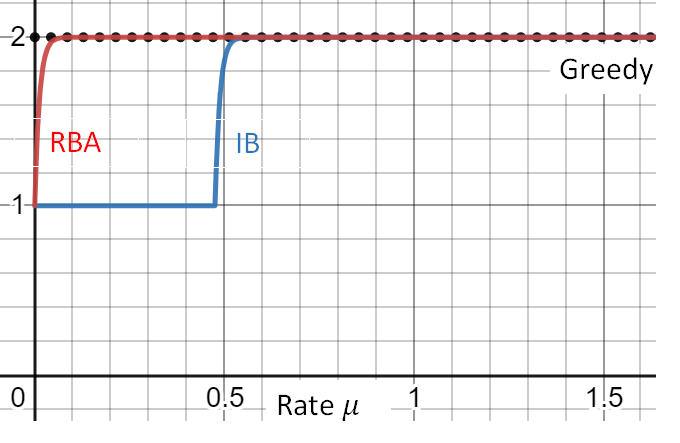
Figure 1: Comparison of Greedy, Balance, and RBA on Example 8.2. Numbers on the $y$ axis denote the resource matched to $t_{0}$ w.h.p..

8.3 Variants of Balance

Examples 8.1 and 8.2 hint at the following “switching” behavior: In phases of arrivals where resources return “frequently” relative to the arriving demand, it is better to be greedy. On the other hand, when arrivals occur in a large batch and resources can not return in time, we should follow Balance to protect diminishing resources. Since we have no information about future arrivals it is not clear how an online algorithm can make this “switch” optimally. While RBA manages to perform this switch quite nimbly, the following natural variants of Balance fail to do so.

1. An algorithm that uses distributional knowledge to deduce when some items are not going to return and refreshes the maximum capacity instead of just the remaining capacity. In the context of Example 8.1, this algorithm would realize after 1 unit of time that the units of resource 1 that have not returned, will never return. Subsequently, it computes a new maximum capacity of $n/2$ for resource 1 at time 1, and treats the resource as if it were at full capacity. It is not hard to see that in general this ends up converging to the greedy algorithm (when the return probabilities approach 0 for instance).

2. An algorithm that anticipates that items are going to return in the future and considers a more optimistic remaining capacity level. In Example 8.1, this algorithm would deduce that there are no further items returning after time 1. Therefore, it makes the same decisions as Balance on the instance in Example 8.1.

9 Connection to Stochastic Rewards Problem

Recall that the stochastic rewards problem of Mehta and Panigrahi (2012) generalizes online matching (with non-reusable resources) by associating a probability of success $p_{it}$ with every edge $(i,t)\in E$. When a match is made i.e., edge is chosen, it succeeds independently with this probability. If the match fails the arrival departs but the resource is available for future rematch.

We introduce an equivalent form of stochastic rewards where the reward is deterministic and independent of the success/failure of matching. Formally, consider the stochastic rewards setting with identical success probability $p$ for every edge and resources with unit reward. We transform this to an instance of the following problem:

Online matching with stochastic consumption: Each edge has a probability $p$ of success. We assume that $p>0$. If an arrival is matched to some resource, we earn a unit reward. After each match, a unit of the matched resource is used forever w.p. $p$, independent of other outcomes. With the remaining probability $1-p$, we do not lose a unit of the resource. Recall, we earn a unit reward in either realization.

We can denote an instance of either of these problems simply as $(G,p)$, where $G$ is the graph and $p>0$ is the edge probability. Now, consider the family of non-anticipative algorithms for these problems, i.e., algorithms (online or offline) that do not know the realization of any match beforehand. Every online algorithm is naturally non-anticipative. Offline algorithms such as the clairvoyant benchmark, as well the stronger fully offline benchmark that can match arrivals in an arbitrary sequence (Goyal and Udwani 2020), are both non-anticipative. Evaluating competitive ratios against non-anticipative offline algorithms, we have the following result.

Lemma I2.

The problem of online matching with stochastic consumption (with probability $p>0$) is equivalent in the competitive ratio sense to the problem of online matching with stochastic rewards and identical edge probabilities, i.e., an $\alpha$ competitive online algorithm in one setting can be translated to an $\alpha$ competitive online algorithm in the other.

Proof.

Consider an instance of the stochastic rewards problem and a non-anticipative algorithm $\mathcal{A}$, that can be offline or online. Consider the alternate reward function where each time $\mathcal{A}$ makes a match we obtain a deterministic reward $p$ regardless of the outcome of the match. Due to non-anticipativity of $\mathcal{A}$ and using the linearity of expectation, the expected total alternative reward of $\mathcal{A}$ is the same as its expected total reward.

Now, consider an instance $(G,p)$ of the (online matching with stochastic) consumption problem with $p>0$. Given algorithm $\mathcal{A}$ for the stochastic rewards problem, we can obtain an algorithm $\mathcal{A}^{\prime}$ for the stochastic consumption problem by simulating $\mathcal{A}$ on a coupled instance $(G,p)$ of the stochastic reward problem. The total expected reward of $\mathcal{A}^{\prime}$ for the consumption problem is $\frac{1}{p}$ times the alternative reward of $\mathcal{A}$ on instance $(G,p)$ for the stochastic rewards problem.

Observe that we can proceed in the reverse direction with similar arguments, i.e., given an algorithm $\mathcal{B}^{\prime}$ for the consumption problem, we can construct an algorithm $\mathcal{B}$ for the stochastic rewards problem via simulating $\mathcal{B}^{\prime}$ on a coupled instance of the consumption problem. The expected reward of $\mathcal{B}$ on an instance $(G,p)$ of the stochastic rewards problem is $p$ times the expected reward of $\mathcal{B}^{\prime}$ on the instance $(G,p)$ of the consumption problem.

Since these arguments hold for both online and offline algorithms, the constant factor of $p$ (or $1/p$) cancels out for $p>0$ and we have the desired competitive ratio equivalence. ∎

Proof.

Proof of Lemma 20. It is now easy to see that the stochastic consumption problem is equivalent to the setting of online matching with reusable resources when the usage distributions for every resource is supported on $\{0,+\infty\}$, with probability of return $1-p$. To make this connection, we simply interpret unsuccessful consumption of a resource in the stochastic consumption setting as the resource returning with duration $0$ in the reusable resources setting, and vice versa. Given this interpretation, we can now directly use an algorithm from one setting in the other setting with the same expected reward. ∎

More generally, consider the stochastic rewards problem with heterogeneous edge probabilities $p_{it}$. The greedy algorithm that matches each arrival to the resource with highest expected reward is $1/2$ competitive for this general problem. Now, consider the corresponding generalization in the reusable resource setting with two point usage distributions supported on $\{0,+\infty\}$ and return probability $1-p_{it}$ for edge $(i,t)$. This problem does not admit any constant factor competitive ratio result (Theorem 2 in Gong et al. (2021)). The proof of equivalence breaks down since the expected reward of a match $(i,t)$ in the stochastic rewards setting is now $p_{it}$. In contrast, the reward for a match in the reusable resource setting is 1, as before. As the ratio between these rewards is now arrival dependent (unlike the case of identical probabilities) it does not cancel out as a constant factor when evaluating the competitive ratios.

10 Validity of Generalized Certificate

Lemma.

Given an online algorithm ALG, non-negative values $\{\lambda_{t}(\omega,\nu)\}_{t,\omega,\nu}$ and $\{\theta_{i}\}_{i}$ such that condition (1) holds and,

$$\theta_{i}+\mathbb{E}_{\boldsymbol{\omega,\nu}}\Big{[}\sum_{t\in P_{i}(\omega,\nu)}\lambda_{t}(\omega,\nu)\Big{]}\geq\alpha_{i}r_{i}\mathbb{E}_{\boldsymbol{\omega}}\Big{[}\sum_{t\in P_{i}(\omega,\nu)}1\Big{]}\quad\forall i\in I,$$ (17)

for some valid collection $P(\omega,\nu)=\{P_{1}(\omega,\nu),\cdots,P_{i}(\omega,\nu)\}$. We have,

$$\textsc{ALG}\geq\frac{\min_{i}\alpha_{i}}{\beta}\textsc{OPT}.$$

Proof.

Proof of Lemma 3. We start by summing over the “pseudo-rewards” (LHS in (17)) over all $i$,

$$\sum_{i}\Big{(}\theta_{i}+\mathbb{E}_{\boldsymbol{\omega,\nu}}\Big{[}\sum_{t\in P_{i}(\omega,\nu)}\lambda_{t}(\omega,\nu)\Big{]}\Big{)} =\sum_{i}\theta_{i}+\mathbb{E}_{\boldsymbol{\omega,\nu}}\Big{[}\sum_{i}\sum_{t\in P_{i}(\omega,\nu)}\lambda_{t}(\omega,\nu)\Big{]}$$

$$\overset{(a)}{\leq}\sum_{i}\theta_{i}+\mathbb{E}_{\boldsymbol{\omega,\nu}}\Big{[}\sum_{t}\lambda_{t}(\omega,\nu)\Big{]}$$

$$\overset{(b)}{=}\sum_{i}\theta_{i}+\sum_{t}\lambda_{t}\leq\beta\textsc{ALG}.$$

Inequality $(a)$ follows from the fact that $P(\omega,\nu)$ is collection of disjoint subsets of $T$. Equality $(b)$ follows by exchanging the order of the sum and expectation and using the definition $\lambda_{t}=\mathbb{E}_{\boldsymbol{\omega,\nu}}[\lambda_{t}(\omega,\nu)]$. Using (17) we have, $\beta\textsc{ALG}\geq\sum_{i}\alpha_{i}\textsc{OPT}_{i}\geq(\min_{i}\alpha_{i})\textsc{OPT}.$ ∎

10.1 Tightness of LP free Certificate

For simplification, consider a deterministic setting and a deterministic online algorithm such that the LP free certificate is given by the following inequalities,

$$\sum_{t\in T}\lambda_{t}+\sum_{i\in I}\theta_{i} \leq \beta\textsc{ALG}$$

$$\sum_{t\in\textsc{OPT}(i)}\lambda_{t}+\theta_{i} \geq \alpha r_{i}\textsc{OPT}_{i}\quad\forall i\in I,$$

$$\lambda_{t},\,\theta_{i}\geq 0.$$

We view this linear system as an LP with a trivial objective of minimizing 0 (a constant). The dual of the LP is

$$\max -\beta\textsc{ALG}\,y+\alpha\,\sum_{i\in I}r_{i}\textsc{OPT}_{i}\,x_{i}$$

s.t. $$0\leq x_{i}\leq y\quad\forall i\in I,$$

$$y\geq 0.$$

The optimal value of this LP is $\max_{y\geq 0}\left[(-\beta\textsc{ALG}+\alpha\,\sum_{i\in I}r_{i}\textsc{OPT}_{i})\,y\right]$. Thus, from strong duality we have that $\textsc{ALG}\geq\frac{\alpha}{\beta}\textsc{OPT}$, if and only if our LP-free system has a feasible solution. This implies that our certificate is tight i.e., if ALG has a competitive ratio guarantee of $\gamma\in(0,1]$, then there exists a feasible solution to our linear system with $\alpha_{i}=1\,\forall i\in I$ and $\beta=1/\gamma$.

11 Missing Details from Proof of Theorem 1

11.1 Properties of $(F,\boldsymbol{\sigma},\boldsymbol{p})$ Random Process

Lemma (Monotonicity Property).

Given a distribution $F$, arrival set $\boldsymbol{\sigma}=\{\sigma_{1},\cdots,\sigma_{T}\}$, and probability sequences $\boldsymbol{p}_{1}=(p_{11},\cdots,p_{1T})$ and $\boldsymbol{p}_{2}=(p_{21},\cdots,p_{2T})$ such that, $p_{1t}\leq p_{2t}$ for every $t\in[T]$, we have,

$$r(F_{i},\boldsymbol{\sigma},\boldsymbol{p}_{1})\leq r(F_{i},\boldsymbol{\sigma},\boldsymbol{p}_{2}).$$

Proof.

Proof of Lemma 5. Suppose the resource is available at some arrival $\sigma_{t}\in\boldsymbol{\sigma}$. Recall that independent of all other randomness in the random process, w.p. $p_{t}$ we switch the resource to in-use at $\sigma_{t}$ and w.p. $1-p_{t}$ the resource stays available till at least the next arrival. Consider an alternative random process where given a set $\boldsymbol{\sigma}$ and probability sequence $\boldsymbol{p}$, we first sample a random subset $\boldsymbol{\sigma}_{\boldsymbol{p}}$ of $\boldsymbol{\sigma}$ as follows: independently for each arrival $\sigma_{t}\in\boldsymbol{\sigma}$, include the arrival in the subset w.p. $p_{t}$. Taking expectation over this random sampling we claim that,

$$\mathbb{E}[r(F_{i},\boldsymbol{\sigma}_{\boldsymbol{p}})]=r(F_{i},\boldsymbol{\sigma},\boldsymbol{p}).$$

This is a direct implication of the fact that an available resource is switched to unavailable independent of other events.

Now, consider random processes $(F_{i},\boldsymbol{\sigma},\boldsymbol{p}_{1})$ and $(F_{i},\boldsymbol{\sigma},\boldsymbol{p}_{2})$ as given in the statement of the lemma. We establish the main claim by using the alternative viewpoint defined above to couple the two processes. To be more precise, we couple the subset sampling stage in the two processes. First, sample a random subset $\boldsymbol{\sigma}_{\boldsymbol{p}_{1}}$ by including each arrival $\sigma_{t}$ with corresponding probability $p_{1t}$. Next, sample subset $\boldsymbol{\sigma}_{\boldsymbol{p}_{2}\backslash\boldsymbol{p}_{1}}$ of $\boldsymbol{\sigma}$ by independently including arrival $\sigma_{t}$ w.p. $p_{2t}-p_{1t}$, for every $\sigma_{t}\in\boldsymbol{\sigma}$. Finally, let $\boldsymbol{\sigma}_{\boldsymbol{p}_{2}}=\boldsymbol{\sigma}_{\boldsymbol{p}_{1}}\cup\boldsymbol{\sigma}_{\boldsymbol{p}_{2}\backslash\boldsymbol{p}_{1}}$. Since for every $t$, $\sigma_{t}\in\boldsymbol{\sigma}_{\boldsymbol{p}_{2}}$ with probability $p_{2t}$ independent of other points in $\boldsymbol{\sigma}_{\boldsymbol{p}_{2}}$, we have,

$$\mathbb{E}[r(F_{i},\boldsymbol{\sigma}_{\boldsymbol{p}_{2}})]=r(F_{i},\boldsymbol{\sigma},\boldsymbol{p}_{2})\text{ and }\mathbb{E}[r(F_{i},\boldsymbol{\sigma}_{\boldsymbol{p}_{1}})]=r(F_{i},\boldsymbol{\sigma},\boldsymbol{p}_{1}).$$

Observe that $\boldsymbol{\sigma}_{\boldsymbol{p}_{1}}\subseteq\boldsymbol{\sigma}_{\boldsymbol{p}_{2}}$ on every sample path. Thus, to finish the proof it suffices to argue that $r(F,\boldsymbol{\sigma}_{1})\leq r(F,\boldsymbol{\sigma}_{2})$ if $\boldsymbol{\sigma}_{1}\subseteq\boldsymbol{\sigma}_{2}$. Consider $(F,\boldsymbol{\sigma}_{1})$ and $(F,\boldsymbol{\sigma}_{2})$ random processes and the straightforward coupling of usage durations where we have a list of i.i.d. samples drawn according to distribution $F$ and each process independently parses this list in order, moving to the next sample whenever the current sample is used and never skipping samples. On any coupled path, the number of transitions made on arrivals in $\boldsymbol{\sigma}_{2}$ is lower bounded by the number of transitions made on arrivals in $\boldsymbol{\sigma}_{1}$, giving us the desired. ∎

Lemma.

Given a $(F,\boldsymbol{\sigma},\boldsymbol{p})$ random process, let $\boldsymbol{\sigma}^{\prime}\subset\boldsymbol{\sigma}$ be a subset of arrivals where the probability of resource being available is zero. Then, the random processes $(F,\boldsymbol{\sigma},\boldsymbol{p})$ and $(F,\boldsymbol{\sigma},\boldsymbol{p}\vee\boldsymbol{1}_{\boldsymbol{\sigma}^{\prime}})$ are equivalent i.e., at every arrival in $\boldsymbol{\sigma}$ the probability that resource is available is the same in both processes.

Proof.

Proof of Lemma 6. It suffices to show the lemma for a subset $\boldsymbol{\sigma}^{\prime}$ consisting of a single arrival. The result for general $\boldsymbol{\sigma}^{\prime}$ then follows by repeated application. Now, let $\sigma_{t}$ denote an arbitrary arrival in $\boldsymbol{\sigma}$ such that w.p. $1$, the resource is in-use when $\sigma_{t}$ arrives. Observe that we can change the probability $p_{t}$ associated with $\sigma_{t}$ arbitrarily, but this does not change the probability of resource being available at $\sigma_{t}$. In particular, w.p. 1, the resource is in-use when $\sigma_{t}$ arrives in the $(F,\boldsymbol{\sigma},\boldsymbol{p}\vee\boldsymbol{1}_{t})$ random process as well. Consequently, the probabilities at other arrivals are unchanged in going from $(F,\boldsymbol{\sigma},\boldsymbol{p})$ to $(F,\boldsymbol{\sigma},\boldsymbol{p}\vee\boldsymbol{1}_{t})$. ∎

Lemma.

The probability of reward at any arrival $\sigma_{t}$ in the $(F,\boldsymbol{\sigma},\boldsymbol{p})$ random process is the same as the fraction of resource available at arrival $\sigma_{t}$ in the fluid counterpart. Consequently, the expected reward in every $(F,\boldsymbol{\sigma},\boldsymbol{p})$ random process is exactly equal to the total reward in the fluid $(F,\boldsymbol{\sigma},\boldsymbol{p})$ process.

Proof.

Proof of Lemma 7. The proof hinges on the fact that in the $(F,\boldsymbol{\sigma},\boldsymbol{p})$ random process, the duration of every state transition is independent of past randomness. We can therefore write a recursive equation for the probability of reward at every arrival. Let $\eta(\sigma_{t})$ denote the probability that the resource is available when $\sigma_{t}\in\boldsymbol{\sigma}$ arrives. We have,

$$\eta(\sigma_{t})=\eta(\sigma_{t-1})\big{(}1-p_{t-1}\big{)}+\sum_{\tau=1}^{t-1}\eta(\sigma_{\tau})p_{\tau}\big{(}F(\sigma_{t}-\sigma_{\tau})-F(\sigma_{t-1}-\sigma_{\tau})\big{)},$$

where $\eta(\sigma_{1})=1$. By forward induction, it is easy to see that this set of equations has a unique solution. Now, if we were to use $\eta(\sigma_{t})$ to represent the fraction of resource available at $\sigma_{t}$ in the fluid process, then we would obtain the same recursive relation with the same starting condition of $\eta(\sigma_{1})=1$. Thus, the probability of resource availability at $\sigma_{t}$ in the random process is exactly equal to the fraction of resource available at $\sigma_{t}$ in the fluid process. Therefore, the expected reward $p_{t}\eta(\sigma_{t})$ from a match occurring at $\sigma_{t}$ in the $(F,\boldsymbol{\sigma},\boldsymbol{p})$ random process equals the reward from consumption at $\sigma_{t}$ in the fluid process. ∎

11.2 Applying Chernoff and Missing Pieces of Theorem 1

Lemma (From Multiplicative Chernoff).

Given integer $\tau>0$, real value $c>0$, independent indicator random variables $\mathbbm{1}(t)$ for $t\in[\tau]$ and $\delta=\sqrt{\frac{2\log c}{c}}$ such that, $\sum_{t=1}^{\tau}\mathbb{E}\left[\mathbbm{1}(t)\right]\leq\frac{c}{1+\delta}.$ We have,

$$\mathbb{P}\left(\sum_{t=1}^{\tau}\mathbbm{1}(t)\geq c\right)\leq\frac{1}{c}.$$

Proof.

Proof of Lemma 9. Let $\mu=\frac{c}{1+\delta}$. Let the condition on total mean hold with equality i.e.,

$$\sum_{t=1}^{\tau}\mathbb{E}\left[\mathbbm{1}(t)\right]=\mu$$

This is w.l.o.g., as we can always add some number of dummy independent binary random variables to make the condition hold with equality. Now applying the standard multiplicative Chernoff bound for binary random variables we have,

$$\mathbb{P}\Big{(}\sum_{t=1}^{\tau}\mathbbm{1}(t)\geq(1+\delta)\mu=c\Big{)}\leq e^{-\frac{\mu\delta^{2}}{2+\delta}}<\frac{1}{c}.$$

∎

12 From Matching to Multi-unit Assortments

In this section we generalize the $(1-1/e)$ result for the following model.

Online Assortments with Multi-unit demand: Customer $t$ requires up to $b_{it}\geq 0$ units of resource $i\in I$. Given an assortment $S$, the customer chooses at most one resource from $S$ with probabilities given by choice model $\phi_{t}$. Let $y_{i}(t)$ denote the number of units of resource $i$ when $t$ arrives. Selection of resource $i$ results in $\min\{y_{i}(t),\,b_{it}\}$ units of resource $i$ being used for an independently drawn duration $d\sim F_{i}$, and a reward $\min\{y_{i}(t),\,b_{it}\}r_{i}$ (results hold even if each of the $b_{it}$ units is used for an independent random duration). The assortment $S$ that we offer must belong to a downward closed feasible set $\mathcal{F}_{t}$. Choice model $\phi_{t}$ and quantities $b_{it}$ are revealed when $t$ arrives.

Similar to the online matching problem, we will work in the large capacity regime. Due to multi-unit (budgeted) allocations this is more accurately the large budget to bid ratio regime, where the parameter,

$$\gamma:=\min_{i\in I,\,t\in T}\frac{c_{i}}{b_{it}},\text{ approaches }+\infty.$$

We compare online algorithms against a clairvoyant algorithm that knows the choice models and quantities $b_{it}$ for all arrivals in advance but makes assortment decisions in order of the arrival sequence and observes (i) realizations of customer choice after showing the assortment and (ii) realizations of usage duration when used units return (same as an online algorithm). Further, in case of assortments we make the standard assumptions (Golrezaei et al. (2014), Rusmevichientong et al. (2020), Gong et al. (2021)) that for every arrival $t\in T$, choice model $\phi_{t}$ satisfies the weak substitution property i.e.,

$$\phi_{t}(S,i)\geq\phi_{t}(S\cup\{j\},i),\quad\forall i,j\not\in S,\,\forall t\in T.$$ (18)

We also assume access to an assortment optimization oracle that takes a choice model $\phi$ and set of feasible solutions $\mathcal{F}$ as input and outputs a feasible revenue maximizing assortment More generally, an $\alpha$ approximate oracle is also acceptable and in this case the competitive ratio guarantee is $(1-1/e)\,\alpha$.

Since we now need to think in terms of sets of resources offered to arrivals, a relatively straightforward way to generalize G-ALG will be to fractionally “match” every arrival to a collection of revenue maximizing assortments/sets, consuming constituent resources in a fluid fashion in accordance with the choice probabilities.

Output: For every arrival $t$, collection of assortments and probabilities $\{A(\eta,t),u(\eta,t)\}_{\eta}$;

Let $g(t)=e^{-t}$, and initialize $Y(k_{i})=1$ for every $i\in I,k_{i}\in[c_{i}]$;

for every new arrival $t$ do

       For every $k_{i}\in[c_{i}]$ and $t\geq 2$, update values

$$Y(k_{i})=Y(k_{i})+\sum_{\tau=1}^{t-1}\Big{(}F_{i}\big{(}a(t)-a(\tau)\big{)}-F_{i}\big{(}a(t-1)-a(\tau)\big{)}\Big{)}y(k_{i},\tau)$$

// Fluid   update of returning capacity

      

      Initialize $S_{t}=\{i\mid(i,t)\in E\}$, values $\eta=0$, and $y(k_{i},t)=0$ for all $i\in S_{t},k_{i}\in[c_{i}]$;

       while $\eta<1$ and $S_{t}\neq\emptyset$ do

             for $i\in S_{t}$ do

                   if $Y(k_{i})=0$ for every $k_{i}\in[c_{i}]$ then remove $i$ from $S_{t}$;

                   else $z_i=\underset{k_i\in [c_i]}{\arg \max }\{k_i\mid Y(k_i)>0\};\text{// }\text{Highest\hspace{0.17em}\hspace{0.17em} available\hspace{0.17em}\hspace{0.17em} unit }$

                  

             end for

            

            $A(\eta,t)=\underset{S\in S_{t}}{\arg\max}\,\sum_{i\in S}b_{it}r_{i}\phi_{t}(S,i)\left(1-g\left(\frac{z_{i}}{c_{i}}\right)\right)$ // Optimal   assortment   with   RBA

             

            $u(\eta,t)=\min\left\{1-\eta,\min_{i\in A(\eta,t)}\frac{Y(z_{i})}{b_{it}\phi_{t}(A(\eta,t),i)}\right\}$ // Fractional assortment

              

             

            

            Update $\eta\to\eta+u(\eta,t)$;

            

            for $i\in A(\eta,t)$ do

                   Update $y(z_{i},t)\to y(z_{i},t)+u(\eta,t)\,b_{it}\,\phi_{t}(A(\eta,t),i)$;  $Y(z_{i})\to Y(z_{i})-y(z_{i},t)$;

                   // Inventory update after fluid customer choice

                  

             end for

            

       end while

      

end for

ALGORITHM 4 Assort G-ALG

Description of Assort G-ALG (Algorithm 4): Observe that the stochasticity due to choice has been converted to its fluid version. Specifically, arrival $t\in T$ is fractionally “matched” to assortments $A(1,t),\cdots,A(m,t)$ for some $m\geq 0$. The weight/fraction of assortment $A(j,t)$ is given by $u(j,t)>0$ and we have, $\sum_{j=1}^{m}u(j,t)\leq 1$. The amount of resource $i$ (fluidly) consumed as a result of this is given by $\sum_{A(j,t)\ni i}u(j,t)\,\phi\big{(}A(j,t),i\big{)}$. The collection of assortments is found by computing the revenue maximizing assortment with reduced prices computed according to RBA rule, as in the case of matching. The values $y(k_{i},t)$ in the algorithm correspond to the total fraction of unit $k_{i}$ that is fluidly chosen by arrival $t$. The weights $u(j,t)$ are chosen to ensure that $y(k_{i},t)$ does not exceed the fraction of $k_{i}$ that was available when $t$ arrived. We assume w.l.o.g. that the oracle that outputs revenue maximizing assortments never includes resources with zero probability of being chosen in the assortment. Interestingly, the performance guarantee of the relaxed online algorithm Assort G-ALG, depends only on $c_{\min}=\min_{i\in I}c_{i}$.

Lemma L3.

For every instance of the online budgeted assortment problem we have,

$$Assort\textsc{ G-ALG}\geq(1-1/e)\,e^{-\frac{1}{c_{\min}}}\,\textsc{OPT}.$$

Proof.

Proof. Note that the sample path $\omega$ now also includes the randomness due to customer choice. Let $O(\omega,i)$ denote the set of all arrivals on sample path $\omega$ in OPT where some units of $i$ are chosen. Since each arrival chooses (possibly multiple units of) at most one resource, we interpret $O(\omega,i)$ as the set of arrivals “matched” to $i$. Let $b(\omega,i,t)$ denote the number of units of $i$ chosen in OPT at arrival $t\in O(\omega,i)$. Let $z_{i}(t^{+})$ be the highest index unit of resource $i$ that has a non-zero fraction available in Assort G-ALG at $t^{+}$. We use the generalized certification with sample path based variables $\lambda_{t}(\omega)$. Given a sample path $\omega$ and resource $i\in I$, we set,

$$\lambda_{t}(\omega)=b(\omega,i,t)r_{i}\bigg{(}1-g\Big{(}\frac{z_{i}(t^{+})}{c_{i}}\Big{)}\bigg{)},$$ (19)

for every arrival $t\in O(\omega,i)$. Let $\lambda_{t}=\mathbb{E}_{\boldsymbol{\omega}}[\lambda_{t}(\omega)]$. Recall that $y(k_{i},t)$ is the total fraction of unit $k_{i}$ that is fluidly chosen by arrival $t$. By definition of Assort G-ALG, we have

$$\lambda_{t}\leq\sum_{i\in I,\,k_{i}\in[c_{i}]}y(k_{i},t)\,r_{i}\left(1-g\left(\frac{k_{i}}{c_{i}}\right)\right),$$

i.e., $\lambda_{t}$ is at most the expected total reward at $t$ in Assort G-ALG calculated with units at their reduced price. Setting $\theta_{i}$ as before (when proving Lemma 4) i.e.,

$$\theta_{i}=c_{i}\left(e^{\frac{1}{c_{i}}}-1\right)r_{i}\sum_{t}\sum_{k\in[c_{i}]}y(k_{i},t)g\Big{(}\frac{k}{c_{i}}\Big{)},$$

we have that condition (1) of the certificate is satisfied with $\beta=e^{1/c_{\min}}$.

The remaining analysis now mimics the proof of Lemma 4. We generalize the basic setup to demonstrate this formally. Let $\mathbbm{1}(\neg k,t^{+})$ indicate that no fraction of unit $k$ is available in Assort G-ALG right after $t$ has been matched. Recall that $\Delta g(k)=g\big{(}\frac{k-1}{c_{i}}\big{)}-g\big{(}\frac{k}{c_{i}}\big{)}$. By definition of $\lambda_{t}$ (see (19)), we have

$$\mathbb{E}_{\boldsymbol{\omega}}\Big{[}\sum_{t\in O(\omega,i)}\lambda_{t}(\omega)\Big{]}\geq(1-1/e)\textsc{OPT}_{i}-r_{i}\mathbb{E}_{\boldsymbol{\omega}}\Big{[}\sum_{t\in O(\omega,i)}b(\omega,i,t)\sum_{k\in[c_{i}]}\Delta g(k)\mathbbm{1}(\neg k,t^{+})\Big{]}.$$

Fix an arbitrary unit $k_{O}$ of $i$ and let $O(\omega,k_{O})$ denote the set of arrivals on sample path $\omega$ in OPT where $k_{O}$ is one of the chosen units of $i$. Note that $O(\omega,k_{O})$ is a subset of $O(\omega,i)$. Using the decomposition above, it suffices to show that,

$$\mathbb{E}_{\boldsymbol{\omega}}\Big{[}\sum_{t\in O(\omega,k_{O})}\sum_{k\in[c_{i}]}\Delta g(k)\mathbbm{1}(\neg k,t^{+})\Big{]}\leq\frac{1}{c_{i}r_{i}}\theta_{i}.$$

The proof of this inequality follows Lemma 4 verbatim. Crucially, we have the following inequalities that complete the proof,

$$\mathbb{E}_{\boldsymbol{\omega}}\Big{[}\sum_{t\in O(\omega,k_{O})}\mathbbm{1}(\neg k,t^{+})\Big{]}\leq r(F_{i},\boldsymbol{s}(k))\leq r(F_{i},\boldsymbol{T},\boldsymbol{p}(k)),$$

where $\boldsymbol{s}(k),\boldsymbol{T},$ and $\boldsymbol{p}(k)$ are as defined in Lemma 4 i.e., $\boldsymbol{s}(k)$ is the ordered set of all arrivals $t$ (arrival times $a(t)$ to be precise) such that $\mathbbm{1}(\neg k,t^{+})=1$ in Assort G-ALG. $\boldsymbol{T}$ is the ordered set of all arrivals. Finally, probabilities $p(k,t)\in\boldsymbol{p}(k)$ are defined as follows: $p(k,t)=0$ if $y(k,t)=0$, otherwise $p(k,t)=\frac{y(k,t)}{\eta(k,t)}$, where $\eta(k,t)$ is the fraction of $k$ available in Assort G-ALG when $t$ arrives. ∎

The main new challenge in turning Assort G-ALG into Sample Assort G-ALG is that we must deal with scenarios where Assort G-ALG directs some mass towards a set $A$ but only a subset of resources in $A$ are available in Sample G-ALG. Recall that in case of matching, if the randomly chosen resource is unavailable we simply leave $t$ unmatched. We could consider a similar approach here whereby if any unit of sampled set $A$ is unavailable then we do not offer $A$. However, this will not preserve the overall revenue in expectation as the probability of every resource in $A$ being available simultaneously is likely to be small. If it were acceptable to offer an assortment with items that are not available in Sample G-ALG then we could also offer the set $A$ as is. The underlying assumption in such a case is that if the arrival chooses an unavailable item then we earn no reward and the arrival simply departs (called static substitution in Ma et al. (2021)). However, in many applications it may not be possible or desirable to offer an assortment where some items are unavailable.

An alternative approach is to offer the subset $S$ of $A$ that is available in Sample G-ALG at $t$. However, this can affect the choice probability for resources $i\in S\cap A$ in non-trivial ways, and thus, affect future availability of resources in a way that is challenging to control. In other words, the concentration bounds that show Sample G-ALG has the same performance as G-ALG for large inventory, will not apply here. Consequently, we need to find a way to display some subsets of $A$ such that, (i) the overall probability of any given resource being allocated is no larger than if we offered $A$ itself and (ii) we do not rely on multiple resources in $A$ being available simultaneously. The main novelty of our approach to tackle this problem will be to switch our perspective from sets of resources back to individual resources. Specifically, for each resource we find the overall probability that the resource is chosen by a given arrival and then use these probabilities as our guideline i.e., given the subset $S\subseteq A$ of resources that is available, we find a new collection of assortments so that for every available resource, the overall probability of the resource being chosen matches this probability in the original collection of assortments in Assort G-ALG. The main idea here is a probability matching, made non trivial by the fact that we are restricted to choice probabilities given by the choice model. We find an iterative polytime algorithm (Algorithm 3) that ensures that the probability of a resource being chosen by an arrival in Sample G-ALG, matches that in Assort G-ALG.

Recall that $\gamma:=\min_{(i,t)\in E}\frac{c_{i}}{b_{it}}$. We are interested in the case where $\gamma\to+\infty$. Note that we assume knowledge of a lower bound on $\gamma$ in Sample Assort G-ALG. Overloading notation, we denote this lower bound also as $\gamma$.

Initialize capacities $y_{i}(0)=c_{i}$ and let $\delta=\sqrt{\frac{2\log\gamma}{\gamma}}$;

for every new arrival $t$ do

      Update capacities $\{y_{i}(t)\}_{i\in I}$ for resources with returning units and let $S_{t}=\{i\mid y_{i}(t)\geq b_{it}\}$;

      Get collection of assortments $\{A(\eta,t),u(\eta,t)\}_{\eta}$ from Assort G-ALG;

      Randomly sample collection $\eta$ w.p. $u(\eta,t)$;

      For sampled $\eta$, let $\mathcal{\hat{A}},\mathcal{\hat{U}}=\text{Probability Match }\Big{(}A(\eta,t)\cap S_{t},\{\frac{1}{1+\delta}\phi_{t}(A,s)\}_{s\in A(\eta,t)\cap S_{t}}\Big{)}$;

      Randomly sample asssortment $\hat{A}_{j}\in\mathcal{\hat{A}}$ with distribution $\mathcal{\hat{U}}$;

      // Assortment may be empty with non-zero probability

     

     Offer $\hat{A}_{j}$ to $t$ and update capacity after $t$ chooses;

     

      end for

ALGORITHM 5 Sample Assort G-ALG

Lemma.

(Lemma 10 restated) Consider a choice model $\phi:2^{N}\times N\to[0,1]$ satisfying the weak substitution property (see (18)), an assortment $A\subseteq N$ belonging to a downward closed feasible set $\mathcal{F}$, a subset $S\subseteq A$ and target probabilities $p_{s}$ such that, $p_{s}\leq\phi(A,s)$ for every $s\in S$. There exists a collection $\mathcal{A}=\{A_{,}\cdots,A_{m}\}$ of $m=|S|$ assortments along with weights $\big{(}u_{i}\big{)}\in[0,1]^{m}$, such that the following properties are satisfied:

1. For every $i\in[m]$, $A_{i}\subseteq S$ and thus, $A_{i}\in\mathcal{F}$.

2. Sum of weights, $\sum_{i\in[m]}u_{i}\leq 1$.

3. For every $s\in S$, $\sum_{A_{i}\ni s}\,u_{i}\,\phi(A_{i},s)=p_{s}$.

Algorithm 3 computes such a collection $\mathcal{A}$ along with weights $(u_{i})$ in $O(m^{2})$ time.

Proof.

Proof of Lemma 10. We give a constructive proof that outlines Algorithm 3 introduced earlier. Let,

$$q^{0}_{s}=\phi(S,s)\text{ and }\zeta^{0}_{s}=\frac{p_{s}}{q^{0}_{s}}\text{ for every $s\in S$.}$$

Observe that $q^{0}_{s}\geq\phi(A,s)\geq p_{s}$, due to substitutability. Thus, $\zeta^{0}_{s}\leq 1$ for every $s\in S$.

Let $s_{1}$ be an element in $S$ with the smallest value $\zeta^{0}_{s_{1}}$. Let $A_{1}=S$ be the first set added to collection $\mathcal{A}$ with $u_{1}=\zeta^{0}_{s_{1}}$, so that $u_{1}\phi(A_{1},s_{1})=p_{s_{1}}$. We will ensure that all subsequent sets added to $\mathcal{A}$ do not include the element $s_{1}$ and this will guarantee condition $(iii)$ for element $s_{1}$. Next, define the set $S^{1}=S\backslash\{s_{1}\}$. Let,

$$q^{1}_{s}=\phi(S^{1},s)\geq q^{0}_{s}\text{ and }\zeta^{1}_{s}=\frac{p_{s}-u_{1}q^{0}_{s}}{q^{1}_{s}}\text{ for every $s\in S^{1}$.}$$

Observe that $\zeta^{1}_{s}\in[0,1]$ for every $s\in S^{1}$. Let $s_{2}$ denote the element with the smallest value $\zeta^{1}_{s_{2}}$, out of all elements in $S^{1}$. If $\zeta^{1}_{s_{2}}=0$ we stop, otherwise we now add the second set $A_{2}=S^{1}$ to the collection with $u_{2}=\zeta^{1}_{s_{2}}$. Inductively, after $i$ iterations of this process, we have added $i$ nested sets $A_{i}\subset A_{i-1}\subset\cdots\subset A_{1}$ to the collection and have the remaining set $S^{i}=A_{i}\backslash\{s_{i}\}$ of $|A|-i$ elements. Define values,

$$q^{i}_{s}=\phi(S^{i},s)\text{ and }\zeta^{i}_{s}=\frac{p_{s}-\sum_{k=1}^{i}u_{k}q^{k-1}_{s}}{q^{i}_{s}}\text{ for every $s\in S^{i}$.}$$

Let $s_{i+1}\in S^{i}$ be the element with the smallest value $\zeta^{i}_{s_{i+1}}$. If $\zeta^{i}_{s_{i+1}}>0$, we add the set $A_{i+1}=S^{i}$ to the collection with $u_{i+1}=\zeta^{i}_{s_{i+1}}$ and continue.

Clearly, this process terminates in at most $m=|S|$ steps, resulting in a collection of size at most $m$. Each step involves updating the set of remaining elements, computing the new values $\zeta^{(\cdot)}_{s}$ and finding the minimum of these values. Thus every iteration requires at most $O(m)$ time and the overall algorithm takes at most $O(m^{2})$ time. Due to the nested nature of the sets and downward closedness of $\mathcal{F}$, condition $(i)$ is satisfied for every set added to the collection. It is easy to verify that condition $(iii)$ is satisfied for every element by induction. We established the base case for element $s_{1}$ in the first iteration. Suppose that the property holds for all elements $s_{1},s_{2},\cdots,s_{i-1}$. Then, by the definition of $u_{i}$ we have for element $s_{i}$,

$$\sum_{j=1}^{i}u_{j}\phi(A_{j},s_{i})=\big{(}p_{s}-\sum_{j=1}^{i-1}u_{j}q^{j-1}_{s_{i}}\big{)}+\sum_{j=1}^{i-1}u_{j}q^{j-1}_{s_{i}}=p_{s_{i}}.$$

Since $s_{i}$ is excluded from all future sets added to the collection, this completes the induction for $(iii)$. Finally, to prove property $(ii)$ it suffices to show that,

$$u_{m}\leq\zeta^{0}_{s_{m-1}}-\sum_{i=1}^{m-1}u_{i},$$

as this immediately implies, $\sum_{i\in[m]}u_{i}\leq\zeta^{0}_{s_{m}}\leq 1$. The desired inequality follows by substituting $u_{m}$ and using the following facts: (i) $q^{j}_{s_{m}}$ is non-decreasing in $j$ due to substitutability, (ii) $u_{i}\geq 0$ for every $i\in[m]$ since we perform iteration $i$ only if $u_{i}=\zeta^{i-1}_{s_{i}}>0$. Therefore,

$$u_{m}=\frac{p_{s_{m}}-\sum_{i=1}^{m-1}u_{i}q^{i-1}_{s_{m}}}{q^{m-1}_{s_{m}}}\leq\frac{p_{s_{m}}-q^{0}_{s_{m}}\sum_{i=1}^{m-1}u_{i}}{q^{0}_{s_{m}}}=\zeta^{0}_{s_{m}}-\sum_{i=1}^{m-1}u_{i}.$$

∎

The probability matching algorithm be executed more efficiently for the commonly used MNL choice model. Using properties of MNL it suffices to sort the resources in order of values $\zeta^{0}_{s}$ in the beginning and this ordering does not change as we remove more and more elements. Each iteration only takes $O(1)$ time and so the process has runtime dominated by sorting a set of size $m=|S|$ i.e., $O(m\log m)$.

Proof.

Proof of Theorem 2.

Recall that $\gamma=\min_{(i,t)\in E}\frac{c_{i}}{b_{it}}$, and $y(k_{i},t)$ is the total fraction of unit $k_{i}$ that is fluidly chosen by arrival $t$ in Assort G-ALG. The proof rests simply on showing that for every $i\in I$ and $t\in T$, at least $c_{i}/\gamma$ $(\geq b_{it})$ units of $i$ are available at $t$ w.p. at least $1-1/\gamma$. Conditioned on this, from Lemma 10 we have that in Sample Assort G-ALG, $i$ is offered to and chosen by arrival $t$ w.p. $\frac{1}{b_{it}(1+\delta)}\sum_{k\in[c_{i}]}y(k,t)$. This implies a lower bound of $\frac{1-1/\gamma}{1+\delta}\sum_{k\in[c_{i}]}y(k,t)$ on the expected reward from $t$ choosing $i$, completing the proof.

Let $x_{it}:=\frac{1}{b_{it}(1+\delta)}\sum_{k\in[c_{i}]}y(k,t)$. To show that $i$ is available at $t$ w.h.p., we first draw out some hidden independence in the events of concern. Recall that if less than $b_{it}$ units of $i$ are available at $t$ then Sample Assort G-ALG does not offer $i$ in any (randomized) assortment to $t$. Otherwise, Probability Matching (Algorithm 3) ensures that $i$ is offered and chosen by arrival $t$ w.p. exactly $x_{it}$. Now, consider the following alternative process at every arrival,

1. Given collection $\{A(\eta,t),u(\eta,t)\}_{\eta}$ from Assort G-ALG, sample assortment $A(\eta,t)$ independently w.p. $\frac{1}{1+\delta}u(\eta,t)$.

2. Offer $A(\eta,t)$ and it customer chooses resource $i$ with insufficient inventory, reject the customer request.

We refer to this alternative process as the static process. Observe that the static process is probabilistically identical to Sample Assort G-ALG, which first checks the inventory of resources and then offers an assortment (after running probability matching). Thus, it suffices to show that in the static process, for every $i\in I$ and $t\in T$, at least $c_{i}/\gamma$ units of $i$ are available at $t$ w.p. at least $1-1/\gamma$.

Now, consider an arbitrary resource $i$ in the static process and let $\mathbbm{1}(i\to t)$ indicate the event that $i$ is offered to and chosen by $t$. W.l.o.g., we independently pre-sample usage durations for every possible match and let $\mathbbm{1}(d_{t}>a(\tau)-a(t))$ indicate that the duration of usage pre-sampled for (a potential) match of $i$ to arrival $t$ is at least $a(\tau)-a(t)$. Let $\gamma_{i}=\frac{c_{i}}{\max_{t^{\prime}\in T}b_{it^{\prime}}}$. Observe that $\gamma_{i}\leq\gamma\,\,\forall i\in I$. The static process never fails to satisfy customer request for resource $i$ if,

$$\sum_{\tau=1}^{t}b_{i\tau}\mathbbm{1}(i\to\tau)\mathbbm{1}(d_{\tau}>a(t)-a(\tau))\leq c_{i}(1-1/\gamma_{i})\quad\forall t\in T.$$

Define binary (not necessarily Bernoulli) random variables $X_{\tau}=\frac{b_{i\tau}}{\max_{t^{\prime}\in T}b_{it^{\prime}}}\mathbbm{1}(i\to\tau)\mathbbm{1}(d_{\tau}>a(t)-a(\tau))$ for all $\tau\leq t-1$. Random variables $X_{\tau}$ are independent of each other as the assortment sampled, customer choice, and the duration of usage are all independently sampled at each arrival (in the static process). From Assort G-ALG, we have the following upper bound on the total expectation,

$$\mu:=\mathbb{E}\Big{[}\sum_{\tau=1}^{t}X_{\tau}\Big{]}=\sum_{\tau=1}^{t}\frac{b_{i\tau}}{\max_{t^{\prime}\in T}b_{it^{\prime}}}\,x_{i\tau}\big{(}1-F_{i}(a(t)-a(\tau))\big{)}\leq\frac{\gamma_{i}}{1+\delta}.$$

Applying the generalized Chernoff bound as stated in Lemma L4, completes the proof. ∎

Lemma L4.

Given integer $\tau>0$, real value $\gamma>0$, independent binary random variables $X_{t}\in\{0,x_{t}\}$ with $x_{t}\in(0,1]\,\,\forall t\in[\tau]$ and $\sum_{t=1}^{\tau}\mathbb{E}\left[X_{t}\right]\leq\frac{\gamma}{1+\delta}$, where $\delta=\sqrt{\frac{2\log\gamma}{\gamma}}$. We have,

$$\mathbb{P}\left(\sum_{t=1}^{\tau}X_{t}>\gamma-1\right)\leq\frac{1}{\gamma}.$$

Proof.

Proof. Consider bernoulli random variables $Y_{t}$ such that $E[Y_{t}]=x_{t}p_{t}\,\,\forall t\in[\tau]$ and $\sum_{t=1}^{\tau}E[Y_{t}]\leq\frac{\gamma}{1+\delta}$. From Lemma 9, we have

$$\mathbb{P}\left(\sum_{t=1}^{\tau}Y_{t}>\gamma-1\right)\leq\frac{1}{\gamma}.$$

The key step in deriving the Chernoff bound that underlies this inequality is the following upper bound on the moment generating function of $Y_{t}$ (Goemans 2015). For $s\geq 0$,

$$E[e^{sY_{t}}]=(x_{t}p_{t})\,e^{s}+(1-x_{t}p_{t})=1+x_{t}p_{t}\,(e^{s}-1)\leq e^{x_{t}p_{t}\,(e^{s}-1)}.$$ (20)

Using this upper bound along with Markov’s inequality and independence of random variables, gives the desired bound. Thus, to show the desired bound for independent (non-Bernoulli) random variables $X_{t}\in\{0,x_{t}\}$ (where $E[X_{t}]=x_{t}p_{t}$), it suffices to establish the upper bound on moment generating functions given by (20). For $s\geq 0$, we have

$$E[e^{sX_{t}}]=p_{t}\,e^{sx_{t}}+(1-p_{t})=1+p_{t}\,(e^{sx_{t}}-1).$$

Unlike (20), here we have the term $x_{t}$ in the exponent. However, for $s\geq 0$, and $x_{t},\,p_{t}\in[0,1]$, we have, $p_{t}\,(e^{sx_{t}}-1)\leq e^{p_{t}x_{t}\,(e^{s}-1)}-1$, giving us the same upper bound as (20). This completes the proof. ∎

13 Missing Details for RBA

13.1 Boundedness of Common IFR Distributions

Given,

$$L_{i}(\epsilon)=\max_{x\geq 0}\frac{F_{i}\big{(}x+F_{i}^{-1}(\epsilon)\big{)}-F_{i}(x)}{\epsilon},$$

we show that RBA is asymptotically $(1-1/e)$ competitive if $L_{i}(\epsilon)\epsilon\to$ as $\epsilon\to 0$. In particular, if $\epsilon L_{i}(\epsilon)$ decreases to 0 as strongly as $O(\epsilon^{\eta})$ for some $\eta>0$, then we have a polynomial convergence rate of $\tilde{O}(c_{i}^{-\frac{\eta}{1+\eta}})$. We show that this holds for many common IFR families (Chapter 2 of Barlow and Proschan (1996)). An approximation for $L(\epsilon)\epsilon$ that eases calculations is given by $\{F^{-1}(\epsilon)\max_{x\geq 0}f(x)\}$ and $F(x)\to O(1)xf(x)$ for small $x$.

• For exponential, uniform and IFR families with non-increasing density: it is easy to see that $L_{i}(\epsilon)=1$ and thus, $\eta=1$. This implies a $\tilde{O}(c_{i}^{-0.5})$ convergence.

• Weibull distributions: This family is characterized by two non-negative parameters $\lambda,k$ with c.d.f. given by, $F(x)=1-e^{(-x/\lambda)^{k}}$ for $x\geq 0$. The family is IFR only for $k\geq 1$. It is easy to see that,

  $$L(\epsilon)\epsilon=O(1)\epsilon^{1/k}.$$

  Hence, for any finite $\lambda,k$ we have $\tilde{O}(c_{i}^{-\frac{1}{1+k}})$ convergence to $(1-1/e)$.

• Gamma distributions: This family is given by non-negative parameters $k,\theta$ such that the c.d.f. is $F(x)=\frac{1}{\Gamma(k)}\gamma(k,x/\theta)$. Here $\Gamma,\gamma$ are the upper and lower incomplete gamma functions resp.. The family is IFR only for $k\geq 1$. It can be shown that for small $\epsilon$, $L(\epsilon)\epsilon\to O(1)\epsilon^{1/k}$. Thus, we have $\tilde{O}(c_{i}^{-\frac{1}{1+k}})$ convergence for any finite set of parameter values.

• Modified Extreme Value Distributions: This family is characterized by the density function, $f(x)=\frac{1}{\lambda}e^{-\frac{e^{x}-1}{\lambda}+x}$ where parameter $\lambda>0$. For small $\epsilon$ we have that $L(\epsilon)\epsilon\to O(1)\epsilon$, for any finite $\lambda$. Giving a a $\tilde{O}(c_{i}^{-0.5})$ convergence.

• Truncated Normal: For truncated normal distribution with finite mean $\mu$, finite variance $\sigma^{2}$, and support $[0,b]$ where $b$ could $\to\infty$, it is easy to see that $L(\epsilon)=O(1)$, leading to a $\tilde{O}(c_{i}^{-0.5})$ convergence. Note that if the support is given by $[a,b]$ for some $a>0$, then we do not have convergence as $L(\epsilon)\epsilon\to O(1)$.

13.2 Proofs of individual components

Lemma.

(Lemma 12 restated) Given $\lambda_{t}$ as defined by (11), we have for every resource $i$,

$$\mathbb{E}_{\boldsymbol{\omega}}\Big{[}\sum_{t\in O(\omega,i)}\lambda_{t}\Big{]}\geq(1-1/e)\textsc{OPT}_{i}-r_{i}\mathbb{E}_{\boldsymbol{\omega}}\Big{[}\sum_{t\in O(\omega,i)}\sum^{c_{i}}_{k=1}\Delta g(k)\mathbb{P}_{\boldsymbol{\nu}}\big{[}k>z_{i}(t)\big{]}\Big{]}.$$

Proof.

Proof of Lemma 12. We start with the LHS,

$$\mathbb{E}_{\boldsymbol{\omega}}\Big{[}\sum_{t\in O(\omega,i)}\lambda_{t}\Big{]} =\mathbb{E}_{\boldsymbol{\omega,\nu}}\Big{[}\sum_{t\in O(\omega,i)}r_{D(t)}[1-g\Big{(}\frac{z_{D(t)}}{c_{D(t)}}\Big{)}]\Big{]},$$ (21)

$$\overset{(a)}{\geq}\mathbb{E}_{\boldsymbol{\omega,\nu}}\Big{[}\sum_{t\in O(\omega,i)}r_{i}[1-g\Big{(}\frac{z_{i}(t)}{c_{i}}\Big{)}]\Big{]},$$

$$\overset{(b)}{=}r_{i}\mathbb{E}_{\boldsymbol{\omega,\nu}}\Big{[}\sum_{t\in O(\omega,i)}\Big{(}1-1/e-\sum_{k=z_{i}(t)+1}^{c_{i}}\Delta g(k)\Big{)}\Big{]},$$

$$\overset{}{=}(1-1/e)\textsc{OPT}_{i}-r_{i}\mathbb{E}_{\boldsymbol{\omega,\nu}}\Big{[}\sum_{t\in O(\omega,i)}\sum_{k=z_{i}(t)+1}^{c_{i}}\Delta g(k)\Big{]},$$

where $(a)$ follows by the fact that RBA matches every arrival to the resource that has maximum reduced price and $(b)$ follows by observing,

$$1-g\Big{(}\frac{z_{i}(t)}{c_{i}}\Big{)}=(1-1/e)-\sum_{k=z_{i}(t)+1}^{c_{i}}\Delta g(k).$$

Finally, we rewrite the $\mathbb{E}_{\boldsymbol{\omega,\nu}}[\cdot]$ term in (21) as follows,

$$\mathbb{E}_{\boldsymbol{\omega,\nu}}\Big{[}\sum_{t\in O(\omega,i)}\sum_{k=z_{i}(t)+1}^{c_{i}}\Delta g(k)\Big{]} =\mathbb{E}_{\boldsymbol{\omega}}\Big{[}\sum_{t\in O(\omega,i)}\mathbb{E}_{\boldsymbol{\nu}}\,\Big{[}\sum^{c_{i}}_{k=z_{i}(t)+1}\Delta g(k)\Big{]}\Big{]},$$ (22)

$$=\mathbb{E}_{\boldsymbol{\omega}}\Big{[}\sum_{t\in O(\omega,i)}\sum^{c_{i}}_{k=1}\Delta g(k)\mathbb{P}_{\boldsymbol{\nu}}\big{[}k>z_{i}(t)\big{]}\Big{]}.$$

∎

Lemma.

(Lemma 13 restated) Let $D(t)$ denote the resource matched to $t$ by RBA. Given arrival $t$ with edge to $i$ let $\mathbbm{1}_{\nu}[k\succeq D(t)]$ denote the event $k\succeq D(t)$ in RBA i.e., RBA would match $k$ to $t$ if it were available when $t$ arrives. Then, the event $\mathbbm{1}_{\nu}[k\succeq D(t)]$ is independent of the usage durations of every unit $w\preceq k$.

Proof.

Proof of Lemma 13. We proceed via contradiction. Assuming the statement is false, consider two sample paths $\nu_{1}$ and $\nu_{2}$ that agree on the the usage durations of all units and resources except units $k^{-}$, where $k^{-}\preceq k$, such that there is an arrival $t$ where $k\succeq D_{1}(t)$ but $k\prec D_{2}(t)$. In fact, suppose $t$ is the earliest arrival where for some unit $k^{+}\succeq k$, we have $k^{+}\succeq D_{1}(t)$ but $k^{+}\prec D_{2}(t)$ (the setting of index 1 or 2 over sample paths is arbitrary). Since the usage duration of all units preceding $k$ are the same on both paths and the matching decisions over these units is consistent prior to arrival $t$, we have that the availability status of units preceding $k$ is the same on both paths when $t$ arrives. Now by definition of RBA, if $t$ is matched to some unit $D_{2}(t)\succ k$ on one path then it will be matched to the same unit on the other path, contradiction. ∎

Lemma.

(Lemma 17 restated) For every resource $i$,

$$\mathbb{E}_{\boldsymbol{\omega}}\Big{[}\sum_{t\in O(\omega,i)}\sum^{c_{i}}_{k=1}\Delta g(k)\mathbb{P}_{\boldsymbol{\nu}}\big{[}k>z_{i}(t)\big{]}\Big{]}\leq\mathbb{E}_{\boldsymbol{\omega}}\Big{[}\sum_{t\in O(\omega,i)}\Big{(}\sum^{c_{i}}_{k=1}\Delta g(k)\mathbb{E}_{\boldsymbol{\nu_{k^{+}}}}\big{[}\mathcal{X}_{k}(\nu_{k^{+}},t)\big{]}\Big{)}\Big{]}+\frac{2}{r_{i}\epsilon_{i}c_{i}}\textsc{OPT}_{i}.$$

Proof.

Proof of Lemma 17. We start with the observation, $\mathbb{P}_{\boldsymbol{\nu}}\big{[}k>z_{i}(t)\big{]}=\mathbb{E}_{\boldsymbol{\nu_{k^{+}}}}\big{[}\mathbb{P}_{\boldsymbol{\nu_{k}}}[k>z_{i}(t)\mid\nu_{k^{+}}]\big{]}$. Using the classification of each arrival $t$ afforded by the covering function, we get,

$$\mathbb{P}_{\boldsymbol{\nu_{k}}}[k>z_{i}(t)\mid\nu_{k^{+}}] =\mathcal{X}_{k}(\nu_{k^{+}},t)\cdot\mathbb{P}_{\boldsymbol{\nu_{k}}}[k>z_{i}(t)\mid\nu_{k^{+}}]$$ (23)

$$\quad+(1-\mathcal{X}_{k}(\nu_{k^{+}},t))\cdot\mathbb{P}_{\boldsymbol{\nu_{k}}}[k>z_{i}(t)\mid\nu_{k^{+}}]$$

$$\leq\mathcal{X}_{k}(\nu_{k^{+}},t)+(1-\mathcal{X}_{k}(\nu_{k^{+}},t))\cdot\mathbb{P}_{\boldsymbol{\nu_{k}}}[k>z_{i}(t)\mid\nu_{k^{+}}],$$

here we use the upper bound of 1 on probability $\mathbb{P}_{\boldsymbol{\nu_{k}}}[k>z_{i}(t)\mid\nu_{k^{+}}]$, for all $t$ that are covered. As an aside from the proof, one might wonder if this is too loose an upper bound which might hurt us later. Typically, it can be shown that if $t$ is covered in $k$ given $\nu_{k^{+}}$, then it is also covered in all units of $i$ preceding $k$, conditioned on corresponding partial sample paths that are consistent with $\nu_{k^{+}}$. So the bound is reasonably tight. Back to the main argument, we now have by substitution,

$$\mathbb{E}_{\boldsymbol{\omega}}\Big{[}\sum_{t\in O(\omega,i)}\sum^{c_{i}}_{k=1}\Delta g(k)\mathbb{P}_{\boldsymbol{\nu}}\big{[}k>z_{i}(t)\big{]}\Big{]}\leq$$

$$\mathbb{E}_{\boldsymbol{\omega}}\Big{[}\sum_{t\in O(\omega,i)}\Big{(}\sum^{c_{i}}_{k=1}\Delta g(k)\mathbb{E}_{\boldsymbol{\nu_{k^{+}}}}\big{[}\mathcal{X}_{k}(\nu_{k^{+}},t)\big{]}\Big{)}\Big{]}+$$

$$\mathbb{E}_{\boldsymbol{\omega}}\Big{[}\sum_{t\in O(\omega,i)}\Big{(}\sum^{c_{i}}_{k=1}\Delta g(k)\mathbb{E}_{\boldsymbol{\nu_{k^{+}}}}\big{[}(1-\mathcal{X}_{k}(\nu_{k^{+}},t))\mathbb{P}_{\boldsymbol{\nu_{k}}}[k>z_{i}(t)\mid\nu_{k^{+}}]\big{]}\Big{)}\Big{]}.$$

The first term in the inequality is as desired. The next lemma (Lemma M5) shows that the second term is further upper bounded by $\frac{1}{r_{i}\epsilon_{i}c_{i}}\textsc{OPT}_{i}$. ∎

Lemma M5.

For any resource $i$ and arrival $t$, given that for any unit $k$ and path $\nu_{k^{+}}$, $\mathcal{X}_{k}(\nu_{k^{+}},t)=0$ implies $\mathbb{P}_{\boldsymbol{\nu_{k}}}[\mathbbm{1}(k,t)=1\mid\nu_{k^{+}}]\geq\epsilon_{i}$, we have that,

$$\sum_{k=1}^{c_{i}}\Delta g(k)\mathbb{E}_{\boldsymbol{\nu_{k^{+}}}}\big{[}(1-\mathcal{X}_{k}(\nu_{k^{+}},t))\cdot\mathbb{P}_{\boldsymbol{\nu_{k}}}[k>z_{i}(t)\mid\nu_{k^{+}}]\big{]}\leq\frac{2}{\epsilon_{i}c_{i}}$$

If $\epsilon_{i}=1$ then the upper bound can be tightened to 0. Consequently,

$$\mathbb{E}_{\boldsymbol{\omega}}\Big{[}\sum_{t\in O(\omega,i)}\Big{(}\sum^{c_{i}}_{k=1}\Delta g(k)\mathbb{E}_{\boldsymbol{\nu_{k^{+}}}}\big{[}(1-\mathcal{X}_{k}(\nu_{k^{+}},t))\mathbb{P}_{\boldsymbol{\nu_{k}}}[k>z_{i}(t)\mid\nu_{k^{+}}]\big{]}\Big{)}\Big{]}\leq\frac{2}{r_{i}\epsilon_{i}c_{i}}\textsc{OPT}_{i}.$$

Proof.

Proof. Let us focus on the first part of the lemma. If $\epsilon_{i}=1$ then, $\mathbb{P}_{\boldsymbol{\nu_{k}}}[k>z_{i}(t)\mid\nu_{k^{+}}]=0$ whenever $\mathcal{X}_{k}(\nu_{k^{+}},t)=0$, giving us the desired. So from here on, we let $\epsilon_{i}<1$. Using $e^{x}\leq 1+x+x^{2}$ for $x\in[0,1]$, we have that,

$$\Delta g(k)\leq(e^{\frac{1}{c_{i}}}-1)\leq 1/c_{i}+1/c_{i}^{2}\leq 2/c_{i}\text{, for $c_{i}\geq 1$.}$$

Therefore, it suffices to show that,

$$\sum_{k=1}^{c_{i}}\mathbb{E}_{\boldsymbol{\nu_{k^{+}}}}\Big{[}(1-\mathcal{X}_{k}(\nu_{k^{+}},t))\cdot\mathbb{P}_{\boldsymbol{\nu_{k}}}[k>z_{i}(t)\mid\nu_{k^{+}}]\Big{]}\leq\frac{1}{\epsilon_{i}}.$$ (24)

The proof relies on establishing that the LHS is upper bounded by the expectation of a geometric r.v. with success probability $\epsilon_{i}$. Fix an arbitrary arrival $t$ and consider the following naturally iterative process for generating sample paths $\nu$.

We sample the usage durations of units one by one in decreasing order of precedence over units as previously defined. Suppose that as we generate $\nu$, we also grow an array ${\bf b}(\nu)$ with binary values. ${\bf b}(\nu)$ is initially an empty array. At the step where usage durations of all units $k^{+}$ that strictly precede unit $k$ of $i$ have been sampled, the covering function $\mathcal{X}_{k}(\nu_{k^{+}},t)$ is well defined. If $t$ is not covered w.r.t. $k$ on the sample path $\nu_{k^{+}}$ generated so far, then we add an entry to the array ${\bf b}$. Next, we sample the durations of $k$ , i.e., generate $\nu_{k}$. This determines the availability of $k$ at arrival $t$. We set the new array entry to 1 if $k$ is available at $t$ and set the entry to 0 otherwise. Thereafter, we move to the next unit dictated by the precedence order. We repeat the same procedure whenever we reach a unit of resource $i$. For all other units, we simply generate a sample path of its usage durations and move to the next unit in order. At the end of the process (after visiting all units in this manner), we add an entry to the end of the array with value 1 so that there is always an entry with value 1 in the array.

For any unit $k$, observe that conditioned on a new array entry being generated when we reach unit $k$, the probability that the entry is 1 is given by $\mathbb{E}_{\boldsymbol{\nu_{k}}}[\mathbbm{1}(k,t)\mid\nu_{k^{+}}]$, which is at least $\epsilon_{i}$. Due to this probability lower bound, the expected number of entries in the array till the first 1, is upper bounded by the expected number of trials till the first success of a geometric r.v. with success probability $\epsilon_{i}$, as desired. Finally, the number of entries in the array before the first 1 is exactly the number of units that are ranked higher than $z_{i}(t)$ and where $t$ is not covered, proving (24). Since (24) holds for every arrival $t$, for any set $S$ of arrivals we have,

$$\sum_{t\in S}\sum_{k=1}^{c_{i}}\Delta g(k)\mathbb{E}_{\boldsymbol{\nu_{k^{+}}}}\big{[}(1-\mathcal{X}_{k}(\nu_{k^{+}},t))\cdot\mathbb{P}_{\boldsymbol{\nu_{k}}}[k>z_{i}(t)\mid\nu_{k^{+}}]\big{]}\leq\frac{2}{\epsilon_{i}c_{i}}|S|.$$

∎

Lemma.

(Lemma 18 restated) For any resource $i$, unit $k$, and path $\nu_{k^{+}}$, we have,

$$\mathbb{E}_{\boldsymbol{\omega}}\Big{[}\sum_{t\in O(\omega,i)}\mathcal{X}_{k}(\nu_{k^{+}},t)\Big{]}\leq c_{i}r\big{(}F_{i},\boldsymbol{s}(\nu_{k^{+}})\big{)}.$$

Consequently,

$$\mathbb{E}_{\boldsymbol{\omega}}\Big{[}\sum_{t\in O(\omega,i)}\Big{(}\sum^{c_{i}}_{k=1}\Delta g(k)\mathbb{E}_{\boldsymbol{\nu_{k^{+}}}}\big{[}\mathcal{X}_{k}(\nu_{k^{+}},t)\big{]}\Big{)}\Big{]}\leq\Big{(}1+\frac{2}{c_{i}}\Big{)}\sum^{c_{i}}_{k=1}\Big{(}g\Big{(}\frac{k}{c_{i}}\Big{)}\cdot\mathbb{E}_{\boldsymbol{\nu_{k^{+}}}}\big{[}r\big{(}F_{i},\boldsymbol{s}(\nu_{k^{+}})\big{)}\big{]}\Big{)}.$$

Proof.

Proof of Lemma 18. Fix an arbitrary unit $k_{O}$ of $i$ in OPT and let $O(\omega,k_{O})$ denote the set of arrivals matched to this unit on sample path $\omega$ in OPT. It suffices to show that,

$$\mathbb{E}_{\boldsymbol{\omega}}\Big{[}\sum_{t\in O(\omega,k_{O})}\mathcal{X}_{k}(\nu_{k^{+}},t)\Big{]}\leq r\big{(}F_{i},\boldsymbol{s}(\nu_{k^{+}})\big{)}.$$ (25)

now, recall that the set $\boldsymbol{s}(\nu_{k^{+}})$ is defined as the set of all covered arrivals on sample path $\nu_{k^{+}}$, i.e., arrivals $t$ for which $\mathcal{X}_{k}(\nu_{k^{+}},t)=1$. Therefore,

$$\mathbb{E}_{\boldsymbol{\omega}}\Big{[}\sum_{t\in O(\omega,k_{O})}\mathcal{X}_{k}(\nu_{k^{+}},t)\Big{]}=\mathbb{E}_{\boldsymbol{\omega}}\Big{[}\big{|}O(\omega,k_{O})\cap\boldsymbol{s}(\nu_{k^{+}})\big{|}\Big{]}.$$

Now the proof of (25) follows by a straightforward application of the two list coupling argument used to prove (9) (Lemma 4). To see the corollary statement, we change the order of summation in the LHS,

$$\mathbb{E}_{\boldsymbol{\omega}}\Big{[}\sum_{t|O(t)=i}\Big{(}\sum^{c_{i}}_{k=1}\Delta g(k)\mathbb{E}_{\boldsymbol{\nu_{k^{+}}}}\big{[}\mathcal{X}_{k}(\nu_{k^{+}},t)\big{]}\Big{)}\Big{]}=\mathbb{E}_{\boldsymbol{\omega}}\Big{[}\sum^{c_{i}}_{k=1}\Delta g(k)\sum_{t|O(t)=i}\mathbb{E}_{\boldsymbol{\nu_{k^{+}}}}\big{[}\mathcal{X}_{k}(\nu_{k^{+}},t)\big{]}\Big{]}.$$

Using $\Big{(}1-\frac{1}{c_{i}}\Big{)}\Delta g(k)\leq\frac{1}{c_{i}}g(k/c_{i})$ completes the proof. ∎

13.3 Proof of Perturbation Property (Proposition 1) for Various Families

13.3.1 $\{d_{i},+\infty\}$ Distributions.

We consider the case where the usage duration for resource $i$ takes a finite value $d_{i}$ w.p. $p_{i}$ and with remaining probability $1-p_{i}$, the unit is never returned. This generalizes both non-reusable resources as well as deterministic reusability. We show inequality (15) for this family of usage distributions. Then using Lemma 19 we have that for any set of values $\{p_{i}\}_{i\in I}$, RBA is $(1-1/e)$ competitive with convergence rate $O(\frac{1}{\sqrt{c_{min}}})$. Focusing on a single resource $i$ with two-point distribution, we show more strongly that regardless of the usage distributions of other resources, condition (2) holds for $i$ with $\alpha_{i}=1-1/e-O(\frac{1}{\sqrt{c_{i}}})$. We can also sharpen the convergence rate to $O\big{(}\frac{\log c_{i}}{c_{i}}\big{)}$, as promised in Table 1. This requires a subtler analysis that will take us away from the outline developed previously. Thus, we include a proof with sharper convergence rate of $O\big{(}\frac{\log c_{i}}{c_{i}}\big{)}$ separately in Appendix 13.4.

Now, to prove (15), fix an arbitrary resource $i$, unit $k$ and path $\nu_{k^{+}}$. For convenience we treat $\epsilon_{i},\kappa_{i}$ as parameters instead of functions. Their relationship with each other and with parameter $c_{i}$ will be determined towards the end when we optimize the convergence rate. First, we claim the following.

Lemma M6.

Any two arrivals $t_{1},t_{2}$ in the set $\boldsymbol{\sigma}(\nu_{k^{+}})$ are such that $|a(t_{1})-a(t_{2})|\geq d_{i}$.

Proof.

Proof. If we are given an ordered set $\boldsymbol{\sigma}(\nu_{k^{+}})$ where this is not true, then consider the earliest pair of contiguous arrivals in $\boldsymbol{\sigma}(\nu_{k^{+}})$ where this is false and note that the probability of $k$ being matched to the later of the two arrivals is 0. So we can remove this arrival from the set w.l.o.g. Repeating this gives a set with the desired property. ∎

The next lemma gives a superset on the set $\boldsymbol{s}(\nu_{k^{+}})$. For a positive value $\epsilon_{i}\in(0,1]$, let $l_{0}\geq 1$ denote the largest integer such that $p^{l_{0}-1}_{i}\geq\epsilon_{i}$. The value of $\epsilon_{i}$, which is also the probability lower bound used in defining the covering function, will be suitably chosen later in order to optimize the convergence rate. If $\boldsymbol{\sigma}(\nu_{k^{+}})$ contains less than $l_{0}$ elements, let $\sigma_{l_{0}}=T$.

Lemma M7.

Define, $\boldsymbol{S}(\nu_{k^{+}})=\{t\mid\exists\sigma_{j}\text{ s.t. }a(t)-a(\sigma_{j})\in[0,d_{i})\text{ or }t\geq\sigma_{l_{0}}\}.$ Then $\boldsymbol{s}(\nu_{k^{+}})\subseteq\boldsymbol{S}(\nu_{k^{+}})$.

Proof.

Proof. For any arrival $t\not\in\boldsymbol{s}(\nu_{k^{+}})$, clearly $t<\sigma_{l_{0}}$. Now, if $k$ has usage duration $d_{i}$ for at least the first $l_{0}-1$ uses, then we claim that $k$ is available at $t$. This would imply that that the probability of $k$ being available at $t$ is at least $p_{i}^{l_{0}-1},$ as desired. To see the claim, note that since $k$ can be matched at most $l_{0}-1$ times prior to any $t<\sigma_{l_{0}}$, and a finite duration for the first $l_{0}-1$ uses of $k$ implies that $k$ is in use precisely during the intervals $\cup_{j=1}^{l_{0}-1}(a(\sigma_{j}),a(\sigma_{j})+d_{i})$, which do not contain $t$ by assumption. Therefore, $k$ is available at $t$ when its first $l_{0}-1$ durations are finite. ∎

It remains to show that, $r\big{(}F_{i},\boldsymbol{S}(\nu_{k^{+}})\big{)}\leq\big{(}1+\kappa_{i}\big{)}r\big{(}F_{i},\boldsymbol{\sigma}(\nu_{k^{+}})\big{)}$.

Proof.

Proof of (15). The proof follows by considering the simple coupling where we sample the same number $l_{f}$ of finite usage durations, for both random processes in question. When the value $l_{f}\leq l_{0}-1$, the number of matches on set $\boldsymbol{S}(\nu_{k^{+}})$ equals the number of matches on $\boldsymbol{\sigma}(\nu_{k^{+}})$. For $l_{f}>l_{0}-1$ we have a higher reward on the LHS, however we also have the following,

$$r\big{(}F_{i},\boldsymbol{S}(\nu_{k^{+}})\big{)}\leq r\big{(}F_{i},\boldsymbol{\sigma}(\nu_{k^{+}})\big{)}+p_{i}^{l_{0}}r\big{(}F_{i},\boldsymbol{S}(\nu_{k^{+}})\big{)}.$$

Applying Lemma 5 then gives us (15), with $\kappa_{i}=\frac{\epsilon_{i}}{1-\epsilon_{i}}$. ∎

Convergence rate: The rate $O\big{(}\frac{1}{\epsilon_{i}c_{i}}+\frac{\epsilon_{i}}{1-\epsilon_{i}}\big{)}$ with $\epsilon_{i}\to 0$ for large $c_{i}$, is optimal for $\epsilon_{i}=\frac{1}{\sqrt{c_{i}}}$. A sharper rate of $O\big{(}\frac{\log c_{i}}{c_{i}}\big{)}$ is shown in Appendix 13.4.

13.3.2 IFR Distributions.

A major advantage in the $\{d_{i},+\infty\}$ case was that if a unit returned after usage, the duration of usage was always $d_{i}$. In other words, we had the additional structure that a returning unit of $i$ in RBA and in OPT was used for the exact same duration and the main question was whether the unit returned at all. More generally, it is not simply a matter of an item returning after use but also the duration of usage. In particular, the probability that an item is available for (potential) $l$-th use is not stated as simply as $p^{l-1}_{i}$. In this section, we address the new issues that arise for continuous IFR distributions.

For convenience we treat $\epsilon_{i},\kappa_{i}$ as parameters instead of functions. Their relationship with each other and with parameter $c_{i}$ will be determined towards the end when we optimize the convergence rate. We use $f_{i}$ to refer to the p.d.f. and $F_{i}$ to refer to the c.d.f.. Recall that the function $L_{i}(\epsilon)$ is defined as the maximum possible value of the ratio $\big{(}F_{i}(x+F_{i}^{-1}(\epsilon))-F_{i}(x)\big{)}/\epsilon$. We will show that when the usage distribution of $i$ is IFR and bounded in the following sense,

$$L_{i}(\epsilon_{i})\epsilon_{i}\to 0\text{ as }\epsilon_{i}\to 0,$$

then RBA is asymptotically $(1-1/e)$ competitive. More specifically, inequality (2) is satisfied with,

$$\alpha_{i}=(1-1/e)-O\bigg{(}\frac{1}{\epsilon_{i}c_{i}}+L_{i}(\epsilon_{i})\epsilon_{i}\log\Big{(}\frac{1}{L_{i}(\epsilon_{i})\epsilon_{i}}\Big{)}\bigg{)}.$$

For distributions where $L_{i}(\epsilon_{i})\epsilon_{i}=O(\epsilon_{i}^{\eta})$ for some $\eta>0$, the optimal rate is thus, $\tilde{O}\Big{(}c^{-\frac{\eta}{1+\eta}}_{i}\Big{)}$. In Appendix 13.1, we evaluate this parameter $\eta$ for some commonly known families of IFR distributions. Observe that for IFR distributions that have non-increasing densities, such as exponential, uniform etc., $L_{i}(\epsilon_{i})=1$ and we have a resulting convergence rate of $O(\log c_{i}/\sqrt{c_{i}})$. In fact, for exponential distributions we will show a stronger convergence rate of $O(1/\sqrt{c_{i}})$.

To prove these claims, let us fix an arbitrary resource $i$, unit $k$, path $\nu_{k^{+}}$. This also fixes the set $\boldsymbol{\sigma}(\nu_{k^{+}})$ of arrivals that $k$ could be matched to in RBA. Since we have fixed $i$, for simplicity we use the abbreviations,

$$\epsilon:=\epsilon_{i},\quad L:=L_{i}(\epsilon_{i}),\quad F:=F_{i}$$

We assume that the density $f_{i}$ is continuous and consequently, let $\delta_{0}$ and $\delta_{L}$ be such that,

$$F(\delta_{0})=\epsilon\quad\text{ and }\quad F(\delta_{L})=L\epsilon,$$

where note that, $L\epsilon\leq 1$ by definition of $L$. Now, we claim that for a $\mathcal{X}_{k}(\nu_{k^{+}},\epsilon,t)$ covering, the following set of arrivals is a superset of $\boldsymbol{s}(\nu_{k^{+}})$,

$$\boldsymbol{S}(\nu_{k^{+}})=\{t\mid a(t)\in[a(\sigma_{j}),a(\sigma_{j})+\delta_{0})\text{ for some }\sigma_{j}\in\boldsymbol{\sigma}(\nu_{k^{+}})\}.$$

Lemma M8.

$\boldsymbol{s}(\nu_{k^{+}})\subseteq\boldsymbol{S}(\nu_{k^{+}}).$

Proof.

Proof. Consider an arrival $t\notin\boldsymbol{S}(\nu_{k^{+}})$. The closest arrival preceding $t$ in $\boldsymbol{\sigma}(\nu_{k^{+}})$, is at least $\delta_{0}$ time before $a(t)$. Using the IFR property, we have that the probability that $k$ switches from being in-use to free between $a(\sigma_{j})$ and $a(\sigma_{j})+\delta_{0}$ is at least $F(\delta_{0})=\epsilon$. ∎

Given this, in order to show (15), we now aim to to show the following lemma and then apply the monotonicity Lemma 5.

Lemma M9.

Given an IFR distribution $F$ and two sets or arrivals $\boldsymbol{S}(\nu_{k^{+}})$ and $\boldsymbol{\sigma}(\nu_{k^{+}})$, with the property that for any arrival $t$ in $\boldsymbol{S}(\nu_{k^{+}})$, there exists an arrival in $\boldsymbol{\sigma}(\nu_{k^{+}})$ that precedes $t$ by at most $\delta_{0}$ time. We have,

$$r\big{(}F,\boldsymbol{S}(\nu_{k^{+}})\big{)}\leq\Bigg{(}1+O\bigg{(}F(\delta_{L})\log\Big{(}\frac{1}{F(\delta_{L})}\Big{)}\bigg{)}\Bigg{)}\,r\big{(}F,\boldsymbol{\sigma}(\nu_{k^{+}})\big{)}.$$

Proof.

Proof. We will show this in two main steps. First, we show for a certain modified distribution $F^{m}$ ($F^{m}_{i}$ to be precise),

$$r\big{(}F,\boldsymbol{S}(\nu_{k^{+}})\big{)}\leq(1+2F(\delta_{L}))r\big{(}F^{m},\boldsymbol{\sigma}(\nu_{k^{+}})\big{)}.$$ (26)

In the second step, we will relate $r(F^{m},A)$ to $r(F,A)$ for any set $A$. The modified distribution $F^{m}$ needs to satisfy a property that we describe next. The exact definition of the distribution will be introduced later in the proof.

Proposition 2.

Given a c.d.f. $F$, we require a modified distribution $F^{m}$ such that, there exists a coupling that generates samples distributed according to $F^{m}$ by using i.i.d. samples from $F$, with the property that for every sample of $F$ that has value $d\geq\delta_{L}$, the coupled sample of $F^{m}$ has value at most $d-\delta_{0}$.

Suppose a distribution $F^{m}$ that satisfies the above property exists and let $\pi:[\delta_{L},+\infty)\to\mathbb{R}^{+}$ be the mapping induced by the coupling, from samples of $F$ to those of $F^{m}$. Then, to show (26), we use the following coupling between $(F,\mathcal{S}(\nu_{k^{+}}))$ and $(F^{m},\boldsymbol{\sigma}(\nu_{k^{+}}))$ random processes. For the rest of the proof, let us refer to these as processes as $R$ and $R^{m}$ resp..

Consider a long list of i.i.d. samples from distribution $F$. Starting with a pointer $P$ at the first sample in the list, every time we have a transition to in-use in process $R$, we draw the sample $P$ is pointing to and move $P$ to the next sample on the list. Thus, pointer $P$ draws from the list in order without skipping over samples. To couple the two processes, we introduce another pointer on the list, $P^{m}$, for process $R^{m}$. Let us call any sample with value at least $\delta_{L}$, a large sample. Other samples are called small samples. Pointer $P^{m}$ starts at the first large sample in the list. Each time $R^{m}$ needs a new sample, we draw the sample pointed to by $P^{m}$ and pass it through the function $\pi(\cdot)$. The output is then passed to process $R^{m}$ and $P^{m}$ moves down the list to the next large sample. If $P$ and $P^{m}$ point to the sample sample and $P$ moves down the list, $P^{m}$ also moves down the list to the next large sample. At every arrival, we first provide a sample, if required, to $R^{m}$ and update $P^{m}$ before moving to $R$. Thus, pointer $P^{m}$ never lags behind $P$. Compared to the coupling used for Lemma 18, there are two important differences. First, here we do rejection sampling by ignoring small values, as $P^{m}$ always skips to the next large sample. Second, we pass the value pointed to by $P^{m}$ through the function $\pi(\cdot)$ before giving the sample to $R^{m}$.

We claim that $P^{m}$ never skips a large sample in the list. We shall prove this by contradiction. Consider the first large sample in the list which is skipped by $P^{m}$, let its position in the list be $q$. Clearly, $q$ is a sample that is used by $R$ otherwise $P^{m}$ would never skip it. Further, $q$ cannot be the first large sample in the list, as the earliest arrival in $\boldsymbol{\sigma}(\nu_{k^{+}})$ is also the first arrival in $\boldsymbol{S}(\nu_{k^{+}})$. Therefore, $R^{m}$ uses the first large sample at least as early as $R$ does. More generally, given that $P^{m}$ never lags $P$, we have that all large samples preceding $q$ were first used in $R^{m}$. Consider the arrival $\sigma_{j}\in\boldsymbol{\sigma}(\nu_{k^{+}})$, where $R^{m}$ uses the large sample immediately preceding $q$ in the list. Due to the fact that function $\pi(\cdot)$ reduces the sample value passed to $R^{m}$ by at least $\delta_{0}$, we claim that $R^{m}$ needs the next large sample , i.e., $q$, before $R$ does. To see the claim, let $s_{j}$ be the arrival in $\boldsymbol{S}(\nu_{k^{+}})$ where $R$ uses the large sample immediately preceding $q$. Observe that $\sigma_{j}$ occurs at least as early as $s_{j}$ due to $P^{m}$ leading $P$ and by the assumption on $q$ being the first sample skipped by $P^{m}$. Now, due to the decrease in sample value resulting from applying $\pi$, we have that in $R^{m}$, $k$ returns to free state after becoming matched to $\sigma_{j}$, at least $\delta_{0}$ time before $k$ returns to free state after getting matched to $s_{j}$ in $R$. Letting $t_{\sigma}$ and $t_{s}$ denote these return times resp., we have, $t_{\sigma}\leq t_{s}-\delta_{0}$. Suppose that the first arrival in $\boldsymbol{S}(\nu_{k^{+}})$ after time $t_{s}$ occurs at time $\tau_{s}$ and the first arrival in $\boldsymbol{\sigma}(\nu_{k^{+}})$ after time $t_{\sigma}$ occurs at time $\tau_{\sigma}$. To establish the claim that $R^{m}$ uses sample pointed by $q$ before $R$ does, it suffices to argue that $\tau_{\sigma}\leq\tau_{s}$. From the definition of set $\boldsymbol{S}(\nu_{k^{+}})$, we have that either $\tau_{s}\in\boldsymbol{\sigma}(\nu_{k^{+}})$ (in which case, we are done) or $\tau_{s}$ is preceded by an arrival in $\boldsymbol{\sigma}(\nu_{k^{+}})$ that occurs in the interval $[\tau_{s}-\delta_{0},\tau_{s})$. Therefore, $t_{\sigma}\leq t_{s}-\delta_{0}\leq\tau_{s}-\delta_{0},$ and we have that $\tau_{\sigma}\leq\tau_{s}$. So $R^{m}$ requires sample $q$ before $R$, which contradicts that $q$ is the first large sample skipped by $P^{m}$. Hence, $P^{m}$ does not skip any large samples. Since $P^{m}$ never lags $P$, we also have that the total number of large samples passed to $R$ is upper bounded by the number of samples passed to $R^{m}$. Let $r^{lg}(F,\boldsymbol{S}(\nu_{k^{+}}))$ denote the expected number of large sample transitions from available to in-use in process $R$. So far we have shown that,

$$r^{lg}(F,\boldsymbol{S}(\nu_{k^{+}}))\leq r(F^{m},\boldsymbol{\sigma}(\nu_{k^{+}})).$$

Next, we claim that,

$$r(F,\boldsymbol{S}(\nu_{k^{+}}))\leq(1+2F(\delta_{L})))r^{lg}(F,\boldsymbol{S}(\nu_{k^{+}})).$$

Consider an arbitrary transition from available to in use in $R$. The probability that duration of this transition is large is $1-F(\delta_{L})$. Thus, the expected contribution from this transition to $r^{lg}(F,\boldsymbol{S}(\nu_{k^{+}}))$ is $1-F(\delta_{L})$. Summing over all transitions, we have the desired. This completes the proof of (26). To finish the main proof it remains to define a modified distribution $F^{m}$ such that Proposition 2 holds and compare the expected rewards of random processes $(F^{m},\boldsymbol{\sigma}(\nu_{k^{+}}))$ with $(F,\boldsymbol{\sigma}(\nu_{k^{+}}))$. This is the focus of the next lemma. ∎

Lemma M10.

Given IFR distribution $F$ and value $\epsilon\in(0,1]$ such that $\epsilon L(\epsilon)\leq 1/2$, there exists a modified distribution $F^{m}$ that satisfies Proposition 2, such that for any given set of arrivals $A$,

$$r(F^{m},A)\leq\Bigg{(}1+O\bigg{(}F(\delta_{L})\log\Big{(}\frac{1}{F(\delta_{L})}\Big{)}\bigg{)}\Bigg{)}r(F,A).$$ (27)

Proof.

Proof. Let us start with the case of exponential distribution as a warm up. We claim that in fact, choosing $F^{m}=F$ suffices in this case. Inequality (27) follows directly for this choice and it remains show that Proposition 2 is satisfied , i.e., prove the existence of a coupling/mapping $\pi$. Consider the following modified density function,

$$f^{m}(x)=\frac{f(x+\delta_{0})}{1-F(\delta_{0})}.$$

$f^{m}=f$ owing to the memoryless property of exponentials. Now, consider the straightforward coupling that samples from $F$ and rejects all samples until the first large sample is obtained, which is reduced by $\delta_{0}$ before it is output. Observe that this process generates samples with distribution $F^{m}$, and satisfies Proposition 2.

For other IFR distributions, it is not clear if $r(F^{m},\boldsymbol{\sigma}(\nu_{k^{+}}))$ and $r(F,\boldsymbol{\sigma}(\nu_{k^{+}}))$ are comparable given the current definition of $F^{m}$. So we introduce a new modified distribution. Define $\delta_{1}$ so that,

$$F(\delta_{1})=1-L\epsilon.$$

Since we started with $\epsilon L\leq 1/2$ for this lemma, we have that $\delta_{L}\leq\delta_{1}$. Now, the new distribution is,

$$f^{m}(x)=\begin{cases*}\frac{1}{1-L\epsilon}f(x)&$x\in[0,\delta_{1}]$\\ 0&$x>\delta_{1}$\end{cases*}$$

So $f^{m}$ is a truncated version of $f$. First, we show that Proposition 2 holds by defining a mapping $\pi$ such that, for every $t\geq\delta_{L}$ we have $F(t)-F(\pi(t))=L\epsilon$. By definition of $L$ and $\epsilon$, this would imply $t-\pi(t)\geq\delta_{0}$.

Consider values $x\in[0,L\epsilon)$ and non-negative $j\in\mathbb{Z}$. Let $t(x,j)=F^{-1}(x+(j+1)L\epsilon)$. Varying $x$ and $j$ we have that $t(x,j)$ takes all possible values in the range $[\delta_{L},+\infty)$. Defining, $\pi(t(x))=F^{-1}(x+jL\epsilon)$, we have that $F(t)-F(\pi(t))=L\epsilon$ for every $t\geq\delta_{L}$, as desired. Finally, the distribution generated by sampling i.i.d. values from $F$ and applying mapping $\pi$ to all large samples (while ignoring all small samples), corresponds to the distribution $F^{m}$ as defined. To show (27), consider the random variable defined as the minimum number of values drawn i.i.d. with density $f^{m}$, such that the sum of the values is at least as large as a single random value that is drawn independently with density $f$. Let $\hat{n}$ denote the expected value of this random variable. Observe that in order to show the main claim it suffices to show that $\hat{n}\leq(1+\gamma)$, where $\gamma=O(L\epsilon\log(1/L\epsilon))$. To show this, let $\mu,\mu^{m}$ denote the mean of $f$ and $f^{m}$ respectively. Recall that $f^{m}$ is a truncated version of $f$. By definition of $f^{m}$ and the IFR property of $f$, we have that,

$$\mu\leq(1-L\epsilon)\cdot\mu^{m}+L\epsilon(\delta_{1}+\mu).$$ (28)

For the time being, we claim $\mu$ is lower bounded as follows,

$$\mu\geq O(1)\cdot\frac{\delta_{1}}{\log(1/L\epsilon)}.$$ (29)

We proceed with the proof assuming (29) holds and prove this claim later. Substituting this inequality in (28) and using the fact that $x\log(1/x)<1$ for $x\in(0,1]$, we get,

$$\mu^{m}\geq O(1)\cdot\frac{\delta_{1}}{\log(1/L\epsilon)}.$$ (30)

Now, to upper bound $\hat{n}$ consider the following coupling: Given a random sample $t$ from $f$, for $t\leq\delta_{1}$ we consider an equivalent sample drawn from $f^{m}$. For durations $t>\delta_{1}$, we draw independent samples from $f^{m}$ until the sum of these samples is at least $t$. Thus, w.p. $(1-L\epsilon)$, we draw exactly one sample from $f^{m}$ and it suffices to show that in the remaining case that occurs w.p. $L\epsilon$, we draw in expectation $O(\log(1/L\epsilon))$ samples from $f^{m}$. Now, given sample $t\geq\delta_{1}$, note that from (30), the expected number of samples drawn from $f^{m}$ before their sum exceeds $\delta_{1}$ is, $O(\log(1/L\epsilon))$. Second, using the IFR property of $f$, we have that the expected number of samples of $f^{m}$ such that the sum of the sample values is at least $t-\delta_{1}$, is upper bounded by $\hat{n}$. Overall, we have the recursive inequality,

$$\hat{n}\leq(1-L\epsilon)+L\epsilon\big{(}O(\log(1/L\epsilon))+\hat{n}\big{)}.$$

The desired upper bound on $\hat{n}$ now follows.

It only remains to show (29). Let $x_{1}$ be such that $1-F(x_{1})=1/2$. Then, let $x_{2}$ be such that $1-F(x_{1}+x_{2})=1/4$. More generally, let $\{x_{1},\cdots,x_{s}\}$ be the set of values such that $1-F(\sum_{j=1}^{s}x_{j})=1/2^{s}$. We let $s$ be the smallest integer greater that equal to $\log(1/L\epsilon)$. Now, the mean $\mu\geq\sum_{j=1}^{s}x_{j}/2^{j}$. Therefore, $\mu/\delta_{1}$ is lower bounded by $\frac{\sum_{j=1}^{s}x_{j}/2^{j}}{\sum_{j=1}^{s}x_{j}}$. While in general this ratio can be quite low, due to the IFR property we have $x_{j}\geq x_{j+1}$ for every $j\geq 1$. Consequently, the minimum value of this ratio is $\frac{O(1)}{s}=\frac{O(1)}{\log(1/L\epsilon)}$, and occurs when all values $x_{j}$ are equal (which incidentally, implies memoryless property). ∎

Convergence rate: We have $\kappa=O\bigg{(}F(\delta_{L})\log\Big{(}\frac{1}{F(\delta_{L})}\Big{)}\bigg{)}=O\big{(}L\epsilon\log(1/L\epsilon)\big{)}.$ Thus, over all rate of convergence for resource $i$ is, $O\bigg{(}\frac{1}{\epsilon_{i}c_{i}}+L_{i}(\epsilon_{i})\epsilon_{i}\log\Big{(}\frac{1}{L_{i}(\epsilon_{i})\epsilon_{i}}\Big{)}\bigg{)}$. Suppose $L_{i}(\epsilon_{i})\epsilon_{i}=O(\epsilon_{i}^{\eta})$ for some $\eta>0$, then the optimal rate is, $\tilde{O}\Big{(}c^{-\frac{\eta}{1+\eta}}_{i}\Big{)}$, where the $\tilde{O}$ hides a $\log c_{i}$ factor.

13.3.3 IFR with Arbitrary Mass at $+\infty$.

In the previous section we, showed that for bounded IFR distributions RBA is asymptotically $(1-1/e)$ competitive. In certain practical scenarios, it may be reasonable to expect that with some probability resource units under use may never return back to the system. We model this by allowing an arbitrary mass at infinity. Specifically, for resource $i$, let $p_{i}$ denote the probability that a usage duration takes value drawn from distribution with c.d.f. $F_{i}$ and with the remaining probability $1-p_{i}$, the duration takes value $+\infty$. In this section, we show that RBA is still asymptotically $(1-1/e)$ competitive for such a mixture of non-increasing IFR usage distributions with arbitrary mass at infinity.

Fix, $i,k,\nu_{k^{+}}$ and define $L$,$\epsilon$, $\delta_{0}$ and $\delta_{L}$ as before. Given set $\boldsymbol{\sigma}(\nu_{k^{+}})$, consider the random process $(F,\boldsymbol{\sigma}(\nu_{k^{+}}))$ and let $\mathbbm{1}(t,{\tt finite})$ indicate the event that $k$ has not hit a $+\infty$ duration at arrival $t$. For a chosen value $\gamma\in(0,1]$ (finalized later to optimize convergence rate), let $\sigma_{l_{f}}$ be the last arrival in $\boldsymbol{\sigma}(\nu_{k^{+}})$ where,

$$\mathbb{E}[\mathbbm{1}(\sigma_{l_{f}},{\tt finite})]\geq\gamma.$$

If no such arrival exists, let $\sigma_{l_{f}}=T$. This implies,

$$\mathbb{E}[\mathbbm{1}(\sigma_{j},{\tt finite})]\geq\gamma\quad\text{for every }\sigma_{j}<\sigma_{l_{f}}\text{ in }\boldsymbol{\sigma}(\nu_{k^{+}}),$$ (31)

and $$\mathbb{E}[\mathbbm{1}(\sigma_{j},{\tt finite})]<\gamma\quad\text{for every }t>\sigma_{l_{f}}.$$ (32)

Using this define the set of arrivals,

$$\boldsymbol{S}(\nu_{k^{+}})=\{t\mid t>\sigma_{l_{f}}\text{ or }\exists\sigma_{j}\in\boldsymbol{\sigma}(\nu_{k^{+}})\text{ s.t. }a(t)\in[a(\sigma_{j}),a(\sigma_{j})+\delta_{0})\}.$$

Lemma M11.

For a $\mathcal{X}_{k}(\nu_{k^{+}},\gamma\epsilon,t)$ covering, we have that the set of covered arrivals satisfies the following relation, $\boldsymbol{s}(\nu_{k^{+}})\subseteq\boldsymbol{S}(\nu_{k^{+}}).$

Proof.

Proof. Consider an arrival $t\notin\boldsymbol{S}(\nu_{k^{+}})$. Clearly, $t<\sigma_{l_{f}}$ and the closest arrival preceding $t$ in $\boldsymbol{\sigma}(\nu_{k^{+}})$, call it $\sigma_{t}$, is at least $\delta_{0}$ time before $a(t)$. From (31), we have that $k$ has not hit a duration of $\infty$ by the time $\sigma_{t}$ arrives, w.p. at least $\gamma$. Conditioned on this, we have from the IFR property that $k$ switches from being in-use to free between $a(\sigma_{j})$ and $a(\sigma_{j})+\delta_{0}$ w.p. at least $F(\delta_{0})=\epsilon$. Together, this implies that the probability that $k$ is free at $t$ is at least $\gamma\epsilon.$ ∎

Lemma M12.

$r\big{(}F,\boldsymbol{S}(\nu_{k^{+}})\big{)}\leq\Big{(}1+O\big{(}L\epsilon\log(1/L\epsilon)\big{)}\Big{)}(1+2\gamma)\,r\big{(}F,\boldsymbol{\sigma}(\nu_{k^{+}})\big{)}.$

Proof.

Proof. The proof requires a combination of the two analyses so far. Consider the truncated set $\boldsymbol{\hat{S}}(\nu_{k^{+}})=\boldsymbol{S}(\nu_{k^{+}})\backslash\{t\mid t>\sigma_{l_{f}}\}.$ First, we have that,

$$r\big{(}F,\boldsymbol{S}(\nu_{k^{+}})\big{)} <r\big{(}F,\boldsymbol{\hat{S}}(\nu_{k^{+}})\big{)}+\gamma r\big{(}F,\boldsymbol{S}(\nu_{k^{+}})\big{)},$$

$$r\big{(}F,\boldsymbol{S}(\nu_{k^{+}})\big{)} \leq(1+2\gamma)r\big{(}F,\boldsymbol{\hat{S}}(\nu_{k^{+}})\big{)},$$

where we used the fact that $\gamma\leq 1$. It suffices to therefore show that,

$$r\big{(}F,\boldsymbol{\hat{S}}(\nu_{k^{+}})\big{)}\leq\Big{(}1+O\big{(}L\epsilon\log(1/L\epsilon)\big{)}\Big{)}r\big{(}F,\boldsymbol{\sigma}(\nu_{k^{+}})\big{)}.$$

Let us condition on the first $l$ transition in each process being finite and the $l+1$-th transition being $\infty$. Then, the resulting expected number of transitions can be compared in the same way as the case of IFR distributions given in Lemma M9, since we now draw independently from an IFR distribution for the first $l$ durations (having conditioned on these durations being finite). This holds for arbitrary $l$. Taking expectation over $l$ then gives the desired. ∎

Convergence rate: We have $\kappa=O\big{(}\gamma+L\epsilon\log(1/L\epsilon)\big{)}$. Moreover, the probability lower bound at uncovered arrivals is actually $\gamma\epsilon$, instead of $\epsilon$. Thus, over all convergence rate for resource $i$ is, $O\bigg{(}\frac{1}{\epsilon_{i}\gamma_{i}c_{i}}+\gamma_{i}+L_{i}(\epsilon_{i})\epsilon_{i}\log\Big{(}\frac{1}{L_{i}(\epsilon_{i})\epsilon_{i}}\Big{)}\bigg{)}$. Suppose $L_{i}(\epsilon_{i})\epsilon_{i}=O(\epsilon_{i}^{\eta})$, then the optimal rate is, $\tilde{O}\Big{(}c^{-\frac{\eta}{1+2\eta}}_{i}\Big{)}$.

13.4 Refined Bound for $\{d_{i},+\infty\}$

The main bottleneck in getting a stronger convergence factor is the need to ensure large enough probability lower bound $\epsilon_{i}$, for uncovered arrivals. In particular, we chose the parameter $l_{0}$ to ensure that $p_{i}^{l_{0}-1}\geq 1/\sqrt{c_{i}}$, and consequently bound the error term $\frac{1}{p_{i}^{l_{0}-1}c_{i}}$ arising out of Lemma M5. Choosing a larger $l_{0}$ would worsen the convergence rate since term designates the contribution from uncovered arrivals in OPT to (12). The separation of contributions from uncovered and covered arrivals makes the analysis tractable in general. It can also be, at least for $\{d_{i},+\infty\}$ distributions, pessimistic from the point of view of convergence to the guarantee. As an extreme but illustrative example, consider a sample path in OPT where a unit $k_{O}$ of $i$ is matched only to arrivals $t$ that occur late and are all uncovered given some unit $k$ and path $\nu_{k^{+}}$ in RBA. Specifically, at each of the arrivals $k_{O}$ is matched to, let the probability of $k$ in RBA  being available (conditioned on $\nu_{k^{+}}$), equal $p_{i}^{l_{0}-1}$. In this case, the contributions to (12) from uncovered arrivals is significant and that part of the analysis is tight, but there is no contribution from covered arrivals in OPT. Thus, the $\theta_{i}$ term could be used to neutralize some of the negative terms arising out of the uncovered arrivals and this would in turn allow us to set a larger value of $l_{0}$. This observation is the key idea behind improving the analysis.

Lemma M13.

For every $i$, (2) is satisfied with $\alpha_{i}=(1-1/e)-O\Big{(}\frac{\log c_{i}}{c_{i}}\Big{)}$.

Proof.

Proof. We start by fixing also an arbitrary unit $k_{O}$ in OPT and show the following inequality,

$$\frac{(1+2/c_{i})}{r_{i}c_{i}}\theta_{i}+\mathbb{E}_{\boldsymbol{\omega}}\Big{[}\sum_{t\mid O(t)=(i,k_{O})}\Big{(}(1-1/e)-\sum^{c_{i}}_{k=1}\Delta g(k)\mathbb{P}_{\boldsymbol{\nu}}\big{[}k>z_{i}(t)\big{]}\Big{)}\Big{]}$$

$$\geq\Big{[}1-1/e-O\Big{(}\frac{\log c_{i}}{c_{i}}\Big{)}\Big{]}\mathbb{E}_{\boldsymbol{\omega}}\Big{[}\big{|}\{t\mid O(t)=(i,k_{O})\}\big{|}\Big{]}.$$ (33)

The proof then follows by linearity of expectation.

To show (33), we start by conditioning on all randomness in OPT arising out of usage durations of resources and units other than unit $k_{O}$ of $i$, as well as any intrinsic randomness in OPT. Let this partial sample path be denoted as $\omega_{-k_{O}}$. This fixes the set of arrivals that $k_{O}$ is matched to if durations of $k_{O}$ are all finite. Let this set be $\Gamma(\omega_{-k_{O}})=\{t_{1}(\omega_{-k_{O}}),t_{2}(\omega_{-k_{O}}),\cdots,t_{l_{f}(\omega_{-k_{O}})}(\omega_{-k_{O}})\}$. Since usage durations of $k_{O}$ are sampled independently, we have that,

$$\mathbb{E}_{\boldsymbol{\omega}}\Big{[}\big{|}\{t\mid O(t)=(i,k_{O})\}\big{|}\Big{]}=\mathbb{E}_{\boldsymbol{\omega_{-k_{O}}}}\Big{[}\sum_{l\geq 1}p_{i}^{l-1}\mathbbm{1}\big{(}l\leq l_{f}(\omega_{-k_{O}})\big{)}\Big{]}$$

Now, define $l_{0}$ as the largest integer such that $p_{i}^{l_{0}-1}\geq\frac{\log c_{i}}{c_{i}}$. On every path $\omega_{-k_{O}}$, it suffices to focus on at most $l_{0}-1$ finite durations for $k_{O}$ as,

$$\sum_{l\geq 1}^{l_{0}}p_{i}^{l-1}\mathbbm{1}\big{(}l\leq l_{f}(\omega_{-k_{O}})\big{)}\geq\Big{(}1-\frac{\log c_{i}}{c_{i}}\Big{)}\sum_{l\geq 1}p_{i}^{l-1}\mathbbm{1}\big{(}l\leq l_{f}(\omega_{-k_{O}})\big{)}.$$

Thus, in order to prove (33) it suffices to show that,

$$\frac{(1+2/c_{i})}{r_{i}c_{i}}\theta_{i}+\mathbb{E}_{\boldsymbol{\omega_{-k_{O}}}}\Big{[}\sum_{l\geq 1}^{l_{0}}p_{i}^{l-1}\mathbbm{1}\big{(}l\leq l_{f}(\omega_{-k_{O}})\big{)}\Big{(}(1-1/e)-\sum^{c_{i}}_{k=1}\Delta g(k)\mathbb{P}_{\boldsymbol{\nu}}\big{[}k>z_{i}(t_{l}(\omega_{-k_{O}}))\big{]}\Big{)}\Big{]}$$

$$\geq\Big{[}1-1/e-O\Big{(}\frac{\log c_{i}}{c_{i}}\Big{)}\Big{]}\mathbb{E}_{\boldsymbol{\omega_{-k_{O}}}}\Big{[}\sum_{l\geq 1}^{l_{0}}p_{i}^{l-1}\mathbbm{1}\big{(}l\leq l_{f}(\omega_{-k_{O}})\big{)}\Big{]}.$$

In fact, it suffices to show more strongly that for every ordered collection $\Gamma=\{t_{1},\cdots,t_{l_{f}}\}$ of arrivals such that any two consecutive arrivals in the set are at least $d_{i}$ time apart and $l_{f}\leq l_{0}$, we have,

$$\sum_{l\geq 1}^{l_{f}}p_{i}^{l-1}\Big{(}\sum^{c_{i}}_{k=1}\Delta g(k)\mathbb{P}_{\boldsymbol{\nu}}\big{[}k>z_{i}(t_{l})\big{]}\Big{)}-\frac{(1+2/c_{i})}{r_{i}c_{i}}\theta_{i}$$

$$=O\Big{(}\frac{\log c_{i}}{c_{i}}\Big{)}\sum_{l\geq 1}^{l_{f}}p_{i}^{l-1}=O\Big{(}\frac{\log c_{i}}{c_{i}}\Big{)}\frac{1-p_{i}^{l_{f}}}{1-p_{i}}.$$ (34)

Now, fix unit $k$, sample path $\nu_{k^{+}}$, and consequently, the set $\boldsymbol{\sigma}(\nu_{k^{+}})$. We classify arrivals $t_{l}\in\Gamma$ into covered and uncovered in a new way, given by a function $\mathcal{Y}_{k}$. Using Lemma M6, we let any two arrivals in $\boldsymbol{\sigma}(\nu_{k^{+}})$ be at least $d_{i}$ time apart. Then,

$t_{l}$ is covered and $\mathcal{Y}_{k}(\nu_{k^{+}},t_{l})=1$ iff there are $l$ or more arrivals preceding $t_{l}$ in $\boldsymbol{\sigma}(\nu_{k^{+}})$.

Using this definition and the decomposition we performed in Lemma 17, we have,

$$\sum_{l\geq 1}^{l_{f}}p_{i}^{l-1}\Big{(}\sum^{c_{i}}_{k=1}\Delta g(k)\mathbb{P}_{\boldsymbol{\nu}}\big{[}k>z_{i}(t_{l})\big{]}\Big{)}\leq$$

$$\sum_{l\geq 1}^{l_{f}}p_{i}^{l-1}\Big{(}\sum^{c_{i}}_{k=1}\Delta g(k)\mathbb{E}_{\boldsymbol{\nu_{k^{+}}}}\big{[}\mathcal{Y}_{k}(\nu_{k^{+}},t_{l})\big{]}\Big{)}+$$ (35)

$$\sum_{l\geq 1}^{l_{f}}p_{i}^{l-1}\Big{(}\sum^{c_{i}}_{k=1}\Delta g(k)\mathbb{E}_{\boldsymbol{\nu_{k^{+}}}}\big{[}(1-\mathcal{Y}_{k}(\nu_{k^{+}},t_{l}))\mathbb{P}_{\boldsymbol{\nu_{k}}}[k>z_{i}(t_{l})\mid\nu_{k^{+}}]\big{]}\Big{)}.$$

Now, for any unit $k$ in RBA, in (35) we may interpret probabilities $p_{i}^{l-1}$ as the probability that at least $l$ durations of $k$ are finite. Then, by definition of the coupling we have that for every path $\nu_{k^{+}}$,

$$\sum_{l\geq 1}^{l_{f}}p_{i}^{l-1}\mathcal{Y}_{k}(\nu_{k^{+}},t_{l})\leq r(F_{i},\boldsymbol{\sigma}(\nu_{k^{+}})).$$

Using the same algebra as the corollary statements in Lemma 18 and Proposition 2 then gives us that,

$$\sum_{l\geq 1}^{l_{f}}p_{i}^{l-1}\Big{(}\sum^{c_{i}}_{k=1}\Delta g(k)\mathbb{E}_{\boldsymbol{\nu_{k^{+}}}}\big{[}\mathcal{Y}_{k}(\nu_{k^{+}},t_{l})\big{]}\Big{)}\leq\frac{(1+2/c_{i})}{r_{i}c_{i}}\theta_{i}.$$

So in order to prove (34), it remains to show that,

$$\sum_{l\geq 1}^{l_{f}}p_{i}^{l-1}\Big{(}\sum^{c_{i}}_{k=1}\Delta g(k)\mathbb{E}_{\boldsymbol{\nu_{k^{+}}}}\big{[}(1-\mathcal{Y}_{k}(\nu_{k^{+}},t_{l}))\mathbb{P}_{\boldsymbol{\nu_{k}}}[k>z_{i}(t_{l})\mid\nu_{k^{+}}]\big{]}\Big{)}=O\Big{(}\frac{\log c_{i}}{c_{i}}\Big{)}\frac{1-p_{i}^{l_{f}}}{1-p_{i}}.$$

To establish this, again fix a unit $k$ and path $\nu_{k^{+}}$ and note that if some arrival $t_{l}$ is uncovered, we have at most $l-1$ arrivals in $\boldsymbol{\sigma}(\nu_{k^{+}})$ preceding $t_{l}$. Therefore, at any uncovered arrival $t_{l}$,

$$\mathbb{P}_{\boldsymbol{\nu_{k}}}[\mathbbm{1}(k,t_{l})=1\mid\nu_{k^{+}}]\geq p_{i}^{l-1}.$$

Then, applying Lemma M5 with $\epsilon_{i}=p_{i}^{l-1}$, we have that for any $p_{i}<1$,

$$\sum_{k=1}^{c_{i}}\Delta g(k)\mathbb{E}_{\boldsymbol{\nu_{k^{+}}}}\big{[}(1-\mathcal{Y}_{k}(\nu_{k^{+}},t_{l}))\cdot\mathbb{P}_{\boldsymbol{\nu_{k}}}[k>z_{i}(t_{l})\mid\nu_{k^{+}}]\big{]}\leq\frac{2}{p_{i}^{l-1}c_{i}},$$

and in case $p_{i}=1$, the RHS equals 0 (which gives us the desired). For $p_{i}<1$, observe that,

$$\sum_{l\geq 1}^{l_{f}}p_{i}^{l-1}\cdot\frac{2}{p_{i}^{l-1}c_{i}}=\frac{2l_{f}}{c_{i}}\quad\text{ and }\quad l_{f}\leq O(\log c_{i})\frac{1-p_{i}^{l_{f}}}{1-p_{i}}\quad\forall l_{f}\leq l_{0},$$

which completes the proof. ∎

13.5 Counterexample for Assortments

Consider three arrivals $t_{1},t_{2},t_{3}$ that come in that order and two resources $\{1,2\}$ with unit reward and unit capacity (example can be generalized to arbitrary capacity). Let resource $2$ be non-reusable. Each arrival has a multinomial logit (MNL) choice model, i.e., probability $\phi(S,i)=\frac{v_{i}}{v_{0}+\sum_{j\in S}v_{j}}$ for $i\in\{1,2\}$ and any set $S$ containing $i$. MNL parameters for arrivals $t_{1}$ and $t_{2}$ are as follows: $v_{1}=100$, $v_{2}=1$ and $v_{0}=0.01$. Arrival $t_{3}$ has $v^{3}_{1}=1$, $v^{3}_{2}=100$ and $v^{3}_{0}=0.01$. Now, consider the actions of RBA on this instance. Observe that RBA offers set $\{1,2\}$ to arrival $t_{1}$ and with probability close to 1, resource $1$ is chosen by this arrival. Suppose that the probability of resource $1$ returning before arrival $t_{2}$ is $p\in(0,1)$ and resource $1$ returns before arrival $t_{3}$ w.p. 1. Then with probability $p$ we offer arrival $t_{2}$ the set $\{1,2\}$ and resource $1$ is chosen again w.h.p.. Subsequently, arrival $t_{3}$ will choose resource $2$ w.h.p., even if resource $1$ returns and is available. In other words, resource $2$ is the most preferred available resource for arrival $t_{3}$ in this case.

On the other hand, consider the scenario where resource $1$ does not return before arrival $t_{2}$. Arrival $t_{2}$ takes resource $2$ w.h.p.. Given that resource $2$ is non-reusable, arrival $t_{3}$ accepts resource 1 w.h.p.. Therefore, whether arrival $t_{3}$ accepts resource $1$ depends not just on whether resource $1$ is available at arrival $t_{3}$, but also on the past usage duration of resource $1$ itself. If resource $1$ returns before arrival $t_{2}$ then arrival $t_{3}$ does not accept resource $1$, otherwise arrival $t_{3}$ accepts resource $1$ w.h.p.. Note that on both sample paths, resource $1$ is available at arrival $t_{3}$. This violates key properties that enable the analysis of RBA for matching (see Corollary 15).

14 Faster Implementations of G-ALG

Executing G-ALG has two main bottlenecks. First, we need to update values $Y(k_{i})$ by taking into account past partial matches of unit $k_{i}$. Second, we may fractionally match every arrival $t$ to many units and in the worst case, to all $\sum_{i\in I}c_{i}$ units. The first issue is somewhat less limiting, as one can in practice continue to update the states during the time between any two arrivals and update states of different units in parallel. The second issue is more important and has a direct impact on the time taken to decide the match for every arrival.

14.1 From Linear to $\log$ Dependence on Capacity

The first approach to improve the runtime of G-ALG is based on the observation that we only need to find an estimate of the index of the highest available unit. In particular, we can geometrically quantize the priority index of units for every resource. The rank of each unit of resource $i$ now takes a value $\lfloor(1+\epsilon)^{j}\rfloor$ for some $j\in\{0,1,\cdots,\lfloor\log_{1+\epsilon}c_{i}\rfloor\}$, where parameter $\epsilon>0$ is a design choice that trades off the runtime with performance guarantee. Larger $\epsilon$ translates to smaller runtime and larger reduction in guarantee.

Since many units of a resource may now have the same index, for the sake of computation we treat all units with the same index as a single ‘unit’. The improvement in runtime is immediate. In each iteration of the while loop (except the last) we decrease the index of the highest available ’unit’ of at least one resource. So for $\epsilon>0$, there are at most $O(\frac{1}{\epsilon}\sum_{i\in I}\log c_{i})$ iterations to match each arrival. To understand the impact on the performance guarantee, notice that the reduced prices, $r_{i}\big{(}1-g(\frac{z_{i}(t)}{c_{i}})\big{)}$, computed for fractionally matching each arrival are off by a factor of at most $(1\pm\epsilon)$ for every resource. To address this in the analysis, we modify the candidate solution for the certificate as follows,

$$\lambda_{t}=\frac{1}{1-\epsilon}\sum_{i\in I}r_{i}\sum_{k\in[c_{i}]}y(k_{i},t)\bigg{(}1-g\Big{(}\frac{k}{c_{i}}\Big{)}\bigg{)}.$$

The value of $\beta$ in condition (1) is now larger by a factor of $(1-\epsilon)^{-1}$. The rest of Lemma 4 follows as is, resulting in an asymptotic guarantee of $(1-\epsilon)(1-1/e)$.

14.2 Capacity Independent Implementation

The second approach rests on the observation that if we could ensure that at each arrival, every unit either has at least a small $\epsilon>0$ fraction available or is completely unavailable, then the number of units any arrival is partially matched to is at most $\frac{1}{\epsilon}$. We implement this idea in G-ALG by treating each unit as unavailable unless at least $\epsilon$ fraction of it is available. Here $\epsilon$ is a design choice; smaller the value, closer the competitive ratio guarantee to $(1-1/e)$ and larger the runtime. In particular, the time to match $t$ now reduces to $O\big{(}\frac{|I|}{\epsilon}\big{)}$, which is within a $\frac{1}{\epsilon}$ factor of the time taken by much simpler Balance and RBA algorithms.

The deterioration in competitive ratio guarantee is more challenging to unravel. Fix a resource $i$ and unit $k$, and recall the ordered set of arrivals $\boldsymbol{s}(k)$ from the analysis of Lemma 4. Roughly speaking, this is the set of arrivals where where unit $k$ is unavailable in G-ALG. Observe that as a consequence of treating available fraction less than $\epsilon$ as unavailable, the set $\boldsymbol{s}(k)$ is now larger. To see the implication of this, define the $(F_{i},\boldsymbol{T},\boldsymbol{p}(k))$ process to capture actions of G-ALG, in the same way as Lemma 4. A key step in Lemma 4 involves showing that the expectation $r(F_{i},\boldsymbol{T},\boldsymbol{p}(k)\cup\boldsymbol{1}_{\boldsymbol{s}(k)})$, is the same as $r(F_{i},\boldsymbol{T},\boldsymbol{p}(k))$. However, as the set $\boldsymbol{s}(k)$ is now larger, this equality does not hold. Therefore, for a suitably defined non-negative valued function $\kappa$, we aim to show the weaker statement,

$$r\big{(}F_{i},\boldsymbol{T},\boldsymbol{p}(k)\cup\boldsymbol{1}_{\boldsymbol{s}(k)}\big{)}\leq\big{(}1+\kappa(\epsilon)\big{)}\,r\big{(}F_{i},\boldsymbol{T},\boldsymbol{p}(k)\big{)},$$ (36)

If true, this would establish $(1-1/e)\big{(}1+\kappa(\epsilon)\big{)}^{-1}$ competitiveness (asymptotically) for G-ALG. Ideally, would like to show inequality (36) with a function $\kappa$ that takes values as small as possible for every $\epsilon$. Recall that for $\epsilon=0$, we showed in Lemma 4 that inequality (36) holds with $\kappa(\epsilon)=0$. However, for non-zero but small $\epsilon$, it is not clear if inequality (36) holds with a small value $\kappa(\epsilon)$ in general.

Interestingly, this inequality has a remarkably strong connection to Proposition 1 in the analysis of RBA. In some sense, it is equivalent to Proposition 1. More concretely, one can show the inequality (36) for the families of usage distributions where we establish validity of Proposition 1 in this paper. For instance, when distribution $F_{i}$ is exponential, inequality (36) holds with the linear function $\kappa(\epsilon)=2\epsilon$, leading to a $O(n/\epsilon)$ algorithm with asymptotic guarantee $(1+\epsilon)^{-1}(1-1/e)$. More generally, we have $k(\epsilon)=\epsilon^{\eta}$ and a $(1+\epsilon^{\eta})^{-1}(1-1/e)$ guarantee for bounded IFR distributions, where $\eta$ is as defined in case of RBA (Appendix 13.1) Note that while the guarantees for RBA hold only for online matching, the guarantee for this modified version of G-ALG holds for budgeted allocation as well as assortment.

15 Miscellaneous

15.1 Impossibility for Stronger Benchmark

For online matching with reusable resources consider the offline benchmark that in addition to the arrival sequence also knows the realizations of all usage durations in advance. The following example illustrates that no non-trivial competitive ratio result is possible against this benchmark.

Consider a setting with $n$ resources. Resources have identical reward and usage distribution. Consider a two point distribution uniformly supported on $\{0,\infty\}$. Suppose we see $n^{2}$ arrivals, each with an edge to all $n$ resources. The expected reward of any online algorithm is at most $2n$, whereas an offline algorithm that knows the realizations of all durations in advance can w.h.p. match all $n^{2}$ arrivals as $n\to\infty$.

15.2 Clairvoyant is Deterministic

Lemma O14.

There exists a deterministic algorithm that is optimal among the class of all offline algorithms that know the entire arrival sequence but match (or decide assortments) in order of arrival and do not know realizations of stochastic elements (usage durations and customer choice) in advance.

Proof.

Proof.Given an arrival sequence the optimal algorithm is given by a dynamic program with the state space given by the number of arrivals remaining and the availability status of the resources, i.e., for each unit, whether it is currently available or in-use and how long it has been in-use for. The decision space of clairvoyant is simply the assortment decision for the current arrival in the sequence. Let $V(t,S_{t})$ denote the optimal value-to-go at arrival $t$ given that the state of resources is $S_{t}$. We use $\mathbbm{1}(i,S_{t})$ to indicate if a unit of $i$ is available in state $S_{t}$ and recall that $\mathcal{F}_{t}$ denotes the set of feasible assortments at $t$. Let $R\left(A,t+1\mid S_{t}\right)$ denote a possible state of the resources at arrival $t+1$, given state $S_{t}$ and assortment $A$ at arrival $t$. Let $p\left(R\left(A,t+1\mid S_{t}\right)\right)$ denote the conditional probability of occurrence for this state and let $\Omega(A,t+1\mid S_{t})$ denote the set of all possible states $R\left(A,t+1\mid S_{t}\right)$. Clearly,

$$V(t,S_{t})=\max_{A\in\mathcal{F}_{t}\mid\mathbbm{1}(i,S_{t})=1,\forall i\in A}\left(R_{t}(A)+\sum_{R\left(A,t+1\mid S_{t}\right)\in\Omega(A,t+1\mid S_{t})}p\left(R\left(A,t+1\mid S_{t}\right)\right)\,V\left(t+1,R(A,t+1\mid S_{t})\right)\right),$$

where $R_{t}(A)=\sum_{i\in A}r_{i}\phi_{t}(A,i)$. At the last arrival $T$, the future value to go (second term in the above sum) is zero and for any given state $S_{T}$ of resources at $T$, the optimal decision at $T$ is simply the (deterministic) solution to a constrained assortment optimization problem. Performing a backward induction using the above equation, we have for any given set of values $V\left(t+1,R(A,t+1\mid S_{t})\right)$, the optimal assortment decision at arrival $t$ is deterministic. ∎

15.3 Clairvoyant Matches Fractional LP for Large Capacities

Consider the following natural LP upper bound for online matching with reusable resources Dickerson et al. (2018), Baek and Ma (2019), Feng et al. (2019),

$$OPT(LP)=\max \sum_{(i,t)\in E}r_{i}y_{it}$$

$$s.t. \sum_{t=1}^{\tau}[1-F_{i}(a(\tau)-a(t))]y_{it}\leq c_{i}\quad\forall\tau\in\{1,\dots,T\},\forall i\in I$$ (37)

$$\sum_{i\in I}y_{it}\leq 1\quad\forall t\in T$$

$$0\leq y_{it}\leq 1\quad\forall t\in T,\quad i\in I$$

Clearly, $\textsc{OPT}\leq\textsc{OPT}(LP)$ and the allocations generated by any algorithm (offline or online) can be converted into a feasible solution for the LP, regardless of $c_{i}$. Perhaps surprisingly, we show that for large $c_{i}$, the solution to this LP can be turned into a randomized clairvoyant algorithm (that does not know the realizations of usage in advance) with nearly the same expected reward, implying that the LP gives a tight asymptotic bound and moreover, all asymptotic competitive ratios shown against the clairvoyant also hold against the LP.

Theorem O15.

Let $c_{\min}=\min_{i\in I}c_{i}$. Then,

$$\textsc{OPT}(LP)\Big{(}1-O\Big{(}\sqrt{\frac{\log c_{\min}}{c_{\min}}}\Big{)}\Big{)}\leq\textsc{OPT}\leq\textsc{OPT}(LP).$$

Hence, for $c_{\min}\to+\infty$, $\textsc{OPT}\to\textsc{OPT}(LP)$.

Proof.

Proof. We focus on the lower bound and more strongly show that every feasible solution of the LP can be turned into an offline algorithm with nearly the same objective value. Let $\{y_{it}\}_{(i,t)\in E}$ be a feasible solution for the LP. Consider the offline algorithm that uses the LP solution as follows,

When $$t i \{y_{it}/(1+2\delta)\}_{i\in I}$$ arrives, sample a resource to offer, according to the distribution ,

where $\delta=\sqrt{\frac{\log c_{\min}}{c_{\min}}}$. Note that if the sampled resource is unavailable, the algorithm leaves $t$ unmatched. Also w.p., $1-\sum_{i\in I}y_{it}$, the algorithm rejects $t$. Since the LP does not use usage durations, the offline algorithm doesn’t either. The critical element to be argued is that the expected reward of this algorithm is roughly the same as the objective value for the feasible solution. This holds due to concentration bounds and the argument closely mimics the proof of Lemma 8. Finally, since this offline algorithm makes matching decisions in order of the arrival sequence and does not know realizations of usage durations in advance, its performance gives a lower bound on the performance of clairvoyant, i.e., OPT. ∎

Remark: This result generalizes naturally to the settings of online assortment and budgeted allocations. In case of assortments we use the Probability Matching algorithm from Appendix 12 to use the concentration bounds.

15.4 Sufficiency of Static Rewards

Lemma O16.

Given an algorithm (online or clairvoyant) for allocation that does not know the realizations of usage durations, the total expected reward of the algorithm is the same if we replace dynamic usage duration dependent rewards functions $r_{i}(\cdot)$ with their static (finite) expectations $r_{i}=\mathbb{E}_{d_{i}\sim F_{i}}[r_{i}(d_{i})]$, for every resource.

Proof.

Proof. Consider arbitrary algorithm $\mathbb{A}$ as described in the lemma statement. Let $\mathbb{B}$ denote an algorithm that mimics the decisions of $\mathbb{A}$ but receives static rewards $r_{i},\,\forall i\in I$ instead. Now, suppose $\mathbb{A}$ successfully allocates resource $i$ to arrival $t$ on some sample path $\omega(t)$ observed thus far. Then, conditioned on observing $\omega(t)$, the expected reward from this allocation is exactly $r_{i}$. More generally, using the linearity of expectation it follows that the total expected reward of $\mathbb{B}$ is the same as that of $\mathbb{A}$.

Note that for algorithms that also know the realization of usage durations in advance, the decision of allocation can depend on usage durations and conditioned on observed sample path $\omega(t)$, the expected reward from successful allocation of $i$ to $t$ need not be $r_{i}$. ∎

15.5 Upper Bound for Deterministic Arrival Dependent Usage

Lemma O17.

Suppose the usage duration is allowed to depend on the arrivals such that a resource $i$ matched to arrival $t$ is used for deterministic duration $d_{it}$ (revealed when $t$ arrives). Then there is no online algorithm with a constant competitive ratio bound when comparing against offline algorithms that know all arrivals and durations in advance.

Proof.

Proof. Using Yao’s minimax, it suffices to show the bound for deterministic online algorithms over a distribution of arrival sequences. For simplicity, suppose we have a single unit of a single resource and a family of arrival sequences $A(j)$ for $j\in[n]$ (the example can be naturally extended to the setting of large capacity). The arrivals in the sequences will be nested so that all arrivals in $A(j)$ also appear in $A(j+1)$. $A(1)$ consists of a single arrival with usage duration of 1. Suppose this vertex arrives at time $0$. $A(2)$ additionally consists of two more arrivals, each with usage duration of $1/2-\epsilon$, arriving at times $\epsilon$ and $1/2$ respectively. More generally, sequence $A(j)$ is best described using a balanced binary tree where every node represents an arrival and the depth of the node determines the usage duration. Each child node has less than half the usage duration ($d/2-\epsilon$) of its parent ($d$). If the parent arrives at time $t$, one child arrives at time $t+\epsilon$ and the other at $t+d/2$. The depth of the tree for sequence $A(j)$ is $j$ (where depth 1 means a single node). Note that the maximum number of arrivals that can be matched in $A(j)$ is $2^{j-1}$.

Let $Z=\sum_{j=1}^{n}2^{j}$. Now, consider a probability distribution over $A(j)$, where probability $p_{j}$ of sequence $A(j)$ occurring is $\frac{2^{n-j+1}}{Z}$. Clearly, an offline algorithm that knows the full sequence in advance can match $2^{j-1}$ arrivals on sequence $A(j)$ and thus, has revenue $n2^{n}/Z=n/2$. It is not hard to see that the best deterministic algorithm can do no better (in expectation over the random arrival sequences) than trying to match all arrivals with a certain time duration. Any such deterministic algorithm has revenue at most $Z/Z=1$. Therefore, we have a competitive ratio upper bound of $n/2$. ∎

References

- Aggarwal et al. (2011) Aggarwal G, Goel G, Karande C, Mehta A (2011) Online vertex-weighted bipartite matching and single-bid budgeted allocations. Proceedings of the twenty-second annual ACM-SIAM symposium on Discrete Algorithms, 1253–1264 (SIAM).
- Alaei et al. (2012) Alaei S, Hajiaghayi M, Liaghat V (2012) Online prophet-inequality matching with applications to ad allocation. Proceedings of the 13th ACM Conference on Electronic Commerce, 18–35.
- Alon et al. (2003) Alon N, Awerbuch B, Azar Y (2003) The online set cover problem. Proceedings of the thirty-fifth annual ACM symposium on Theory of computing, 100–105.
- Andrews et al. (2019) Andrews JM, Farias VF, Khojandi AI, Yan CM (2019) Primal–dual algorithms for order fulfillment at urban outfitters, inc. Interfaces 49(5):355–370.
- Aouad and Saban (2020) Aouad A, Saban D (2020) Online assortment optimization for two-sided matching platforms. Available at SSRN .
- Azar et al. (1994) Azar Y, Broder AZ, Karlin AR (1994) On-line load balancing. Theoretical computer science 130(1):73–84.
- Azar et al. (1993) Azar Y, Kalyanasundaram B, Plotkin S, Pruhs KR, Waarts O (1993) Online load balancing of temporary tasks. Workshop on algorithms and data structures, 119–130 (Springer).
- Baek and Ma (2019) Baek J, Ma W (2019) Bifurcating constraints to improve approximation ratios for network revenue management with reusable resources. Available at SSRN .
- Bansal et al. (2015) Bansal N, Buchbinder N, Madry A, Naor J (2015) A polylogarithmic-competitive algorithm for the k-server problem. Journal of the ACM (JACM) 62(5):1–49.
- Barlow and Proschan (1996) Barlow RE, Proschan F (1996) Mathematical theory of reliability (SIAM).
- Besbes et al. (2020) Besbes O, Elmachtoub AN, Sun Y (2020) Pricing analytics for rotable spare parts. INFORMS Journal on Applied Analytics 50(5):313–324.
- Birnbaum and Mathieu (2008) Birnbaum B, Mathieu C (2008) On-line bipartite matching made simple. ACM SIGACT News 39(1):80–87.
- Blum et al. (1999) Blum A, Burch C, Kalai A (1999) Finely-competitive paging. 40th Annual Symposium on Foundations of Computer Science (Cat. No. 99CB37039), 450–457 (IEEE).
- Buchbinder et al. (2007) Buchbinder N, Jain K, Naor JS (2007) Online primal-dual algorithms for maximizing ad-auctions revenue. European Symposium on Algorithms, 253–264 (Springer).
- Cruise et al. (2020) Cruise J, Jonckheere M, Shneer S (2020) Stability of jsq in queues with general server-job class compatibilities. Queueing Systems 95:271–279.
- Dean et al. (2005) Dean BC, Goemans MX, Vondrák J (2005) Adaptivity and approximation for stochastic packing problems. Proceedings of the sixteenth annual ACM-SIAM symposium on Discrete algorithms, 395–404.
- Delong et al. (2021) Delong S, Farhadi A, Niazadeh R, Sivan B (2021) Online bipartite matching with reusable resources. arXiv preprint arXiv:2110.07084 .
- Devanur and Hayes (2009) Devanur NR, Hayes TP (2009) The adwords problem: online keyword matching with budgeted bidders under random permutations. Proceedings of the 10th ACM conference on Electronic commerce, 71–78 (ACM).
- Devanur et al. (2013) Devanur NR, Jain K, Kleinberg RD (2013) Randomized primal-dual analysis of ranking for online bipartite matching. Proceedings of the twenty-fourth annual ACM-SIAM symposium on Discrete algorithms, 101–107 (Society for Industrial and Applied Mathematics).
- Devanur et al. (2019) Devanur NR, Jain K, Sivan B, Wilkens CA (2019) Near optimal online algorithms and fast approximation algorithms for resource allocation problems. J. ACM 66(1), ISSN 0004-5411, URL http://dx.doi.org/10.1145/3284177.
- Devanur et al. (2012) Devanur NR, Sivan B, Azar Y (2012) Asymptotically optimal algorithm for stochastic adwords. Proceedings of the 13th ACM Conference on Electronic Commerce, 388–404.
- Dickerson et al. (2018) Dickerson JP, Sankararaman KA, Srinivasan A, Xu P (2018) Allocation problems in ride-sharing platforms: Online matching with offline reusable resources. Thirty-Second AAAI Conference on Artificial Intelligence.
- Feldman et al. (2009a) Feldman J, Korula N, Mirrokni V, Muthukrishnan S, Pál M (2009a) Online ad assignment with free disposal. International workshop on internet and network economics, 374–385 (Springer).
- Feldman et al. (2009b) Feldman J, Mehta A, Mirrokni V, Muthukrishnan S (2009b) Online stochastic matching: Beating 1-1/e. Foundations of Computer Science, 2009. FOCS’09. 50th Annual IEEE Symposium on, 117–126 (IEEE).
- Feng et al. (2019) Feng Y, Niazadeh R, Saberi A (2019) Linear programming based online policies for real-time assortment of reusable resources. Available at SSRN 3421227 .
- Feng et al. (2020) Feng Y, Niazadeh R, Saberi A (2020) Near-optimal bayesian online assortment of reusable resources. Available at SSRN: https://ssrn.com/abstract=3714338 .
- Feng et al. (2021) Feng Y, Niazadeh R, Saberi A (2021) Online assortment of reusable resources with exogenous replenishment. Available at SSRN 3795056 .
- Goel and Mehta (2008) Goel G, Mehta A (2008) Online budgeted matching in random input models with applications to adwords. Proceedings of the nineteenth annual ACM-SIAM symposium on Discrete algorithms, 982–991 (Society for Industrial and Applied Mathematics).
- Goemans (2015) Goemans M (2015) Chernoff bounds, and some applications. URL http://math. mit. edu/goemans/18310S15/chernoff-notes. pdf .
- Golrezaei et al. (2014) Golrezaei N, Nazerzadeh H, Rusmevichientong P (2014) Real-time optimization of personalized assortments. Management Science 60(6):1532–1551.
- Gong et al. (2021) Gong XY, Goyal V, Iyengar G, Simchi-Levi D, Udwani R, Wang S (2021) Online assortment optimization with reusable resources. Management Science (Forthcoming) .
- Goyal and Udwani (2020) Goyal V, Udwani R (2020) Online matching with stochastic rewards: Optimal competitive ratio via path based formulation. Proceedings of the 21st ACM Conference on Economics and Computation, 791, EC ’20.
- Huang and Zhang (2020) Huang Z, Zhang Q (2020) Online primal dual meets online matching with stochastic rewards: configuration lp to the rescue. Proceedings of the 52nd Annual ACM SIGACT Symposium on Theory of Computing, 1153–1164.
- Kalyanasundaram and Pruhs (2000) Kalyanasundaram B, Pruhs KR (2000) An optimal deterministic algorithm for online b-matching. Theoretical Computer Science 233(1-2):319–325.
- Karande et al. (2011) Karande C, Mehta A, Tripathi P (2011) Online bipartite matching with unknown distributions. Proceedings of the forty-third annual ACM symposium on Theory of computing, 587–596 (ACM).
- Karp et al. (1990) Karp RM, Vazirani UV, Vazirani VV (1990) An optimal algorithm for on-line bipartite matching. Proceedings of the twenty-second annual ACM symposium on Theory of computing, 352–358 (ACM).
- Ma et al. (2021) Ma W, Simchi-Levi D, Zhao J (2021) Dynamic pricing (and assortment) under a static calendar. Management Science 67(4):2292–2313.
- Manshadi et al. (2012) Manshadi VH, Gharan SO, Saberi A (2012) Online stochastic matching: Online actions based on offline statistics. Mathematics of Operations Research 37(4):559–573.
- Megow et al. (2006) Megow N, Uetz M, Vredeveld T (2006) Models and algorithms for stochastic online scheduling. Mathematics of Operations Research 31(3):513–525.
- Mehta and Panigrahi (2012) Mehta A, Panigrahi D (2012) Online matching with stochastic rewards. Foundations of Computer Science (FOCS), 2012 IEEE 53rd Annual Symposium on, 728–737 (IEEE).
- Mehta et al. (2007) Mehta A, Saberi A, Vazirani U, Vazirani V (2007) Adwords and generalized online matching. J. ACM 54(5):22–es, ISSN 0004-5411.
- Mehta et al. (2015) Mehta A, Waggoner B, Zadimoghaddam M (2015) Online stochastic matching with unequal probabilities. Proceedings of the twenty-sixth annual ACM-SIAM symposium on Discrete algorithms, 1388–1404 (Society for Industrial and Applied Mathematics).
- Mehta et al. (2013) Mehta A, et al. (2013) Online matching and ad allocation. Foundations and Trends® in Theoretical Computer Science 8(4):265–368.
- Rusmevichientong et al. (2020) Rusmevichientong P, Sumida M, Topaloglu H (2020) Dynamic assortment optimization for reusable products with random usage durations. Management Science 66(7):2820–2844.
- Udwani (2021a) Udwani R (2021a) Adwords with unknown budgets. arXiv preprint arXiv:2110.00504 .
- Udwani (2021b) Udwani R (2021b) Periodic reranking for online matching of reusable resources. arXiv preprint arXiv:2110.02400 .
- Weng et al. (2020) Weng W, Zhou X, Srikant R (2020) Optimal load balancing with locality constraints. Proc. ACM Meas. Anal. Comput. Syst. 4(3):45:1–45:37.
[sections] \printcontents[sections]l1