Scheme for realizing quantum dense coding via entanglement swapping

Abstract

Quantum dense coding is a protocol for transmitting two classical bits of information from a sender (Alice) to a remote receiver (Bob) by sending only one quantum bit (qubit). In this article, we propose an experimentally feasible scheme to realize quantum dense coding via entanglement swapping in a cavity array containing a certain number of two-level atoms. Proper choice of system parameters such as atom-cavity couplings and inter-cavity couplings allows perfect transfer of information. A high fidelity transfer of information is shown to be possible by using recently achieved experimental values in the context of photonic crystal cavities and superconducting resonators. To mimic experimental imperfections, disorder in both the coupling strengths and resonance frequencies is considered.

Keywords: Quantum dense coding, cavity array, cavity-QED

1 Introduction

Quantum dense coding is an important task for realizing quantum communication [1]. It is a process of transmitting two classical bits of information from a sender (Alice) to a remote receiver (Bob) by sending only one qubit. This requires entanglement as an important resource. Due to potential application of quantum dense coding in quantum communication, a lot of attention has been paid to realizing this protocol in many physical systems such as optical systems [2, 3], spin chains [4, 5, 6, 7], cavity quantum electrodynamics (QED) systems [8, 9, 10, 11, 12, 13], etc.

In the context of cavity QED, precise control of the system parameters makes the system as a promising candidate for realizing quantum information processing [14]. Recently, a certain number of atoms dispersively interacting with a single cavity is shown to be a physical system capable of realizing quantum dense coding [9, 12, 8, 11, 13, 15]. The importance of the dispersive coupling is to suppress the effect of dissipation. In this configuration, Alice sends her atomic qubit to Bob for further processing to retrieve the information. On the other hand, Xue et. al. proposed a scheme where the atom is taken as stationary qubit and the photon is used as a flying qubit in free space [10].

Due to recent progress in fabrication, it is possible to realize cavities with high quality ($Q$) factor. With the possibility of precise control of resonance frequencies and coupling strengths of the array, coupled cavities provide a suitable physical system for realizing many quantum information protocols [16, 17, 18, 19, 20, 21, 22, 23]. The scalability of the array is an additional advantage for realizing distance communication. Cavities have been used to realize many interesting phenomena such as entanglement generation [24, 25, 26, 27], nonclassical state preparation [28, 29, 30, 31, 32], localization-delocalization [33, 34], heat transfer [35, 36, 37], photon blockade [38, 39, 40, 41, 42] etc by properly tuning the resonance frequencies or including material medium inside it. In addition, suitable choices of coupling strengths between the cavities provide perfect transfer of photons between the cavities [16, 17, 43, 44].

In this article, we proposed a scheme to realize quantum dense coding protocol in an atom-cavity system. The system consists of a cavity array, and each end cavity of the array contains a two-level atom which is accessible by Alice and Bob respectively. Bob has an additional atom which is entangled with the atom of Alice. Hence, Alice has only one atom whereas Bob has two atoms. In order to transfer the information, Alice encodes the information on her qubit (atom) by applying a unitary transformation. Then, Alice allows her qubit to interact with the cavity array. If the cavity-cavity and the atom-cavity coupling strengths are properly chosen, the entanglement between Alice’s and Bob’s qubits transferred to both the qubits of Bob. At this point, Alice’s and Bob’s qubits are disentangled where as Bob’s qubits are entangled. This is referred to as entanglement swapping in the literature [45, 46, 47]. Here the cavity array acts as a quantum channel and photon as the information carrier. Hence, the time scale for information transfer depends on the inter-cavity coupling strengths. We find that the fidelity of the transfer of two bits of classical information from Alice to Bob is unity in the absence of dissipation. The master equation is employed to calculate the fidelity in the presence of dissipation. Using the experimentally achievable values in the context of photonic crystal cavities and superconducting resonators, we show that the fidelity of information transfer is high. To mimic experimental imperfection, disorder is included in the system.

This article is organized as follows: In Sec. 2, we describe our physical system and provide the choices of coupling strengths for the perfect transfer of information. Quantum dense coding via coupled cavity array is presented in Sec. 3. We discuss the results obtained by using experimentally achievable values of the system parameters in Sec. 4. Finally, we summarized our results in Sec. 5.

2 Physical system

We consider an array of $N$ coupled cavities as shown in Fig. 1. The end cavities of the array contain two two-level atoms $q_{1}$ and $q_{2}$. Alice can control qubit $q_{1}$ which is present in the first cavity and Bob can control $q_{2}$ which is present in the $N$th cavity. In addition, Bob has another qubit $(q_{3})$ in $(N+1)$th cavity, which is separated from the array. We assume that qubit $q_{3}$ does not interact with the $(N+1)$th cavity. Then the Hamiltonian for this system is

$$H =\sum_{i=1}^{3}\omega_{qi}(\sigma_{+}\sigma_{-})_{qi}+\omega\sum_{k=1}^{N+1}a_{k}^{\dagger}a_{k}$$

$$+\sum_{k=1}^{N-1}J_{k}(a_{k}^{\dagger}a_{k+1}+a_{k}a_{k+1}^{\dagger})+g[a_{1}^{\dagger}(\sigma_{-})_{q1}+a_{1}(\sigma_{+})_{q1}]$$

$$+g[a_{N}^{\dagger}(\sigma_{-})_{q2}+a_{N}(\sigma_{+})_{q2}],$$ (1)

where $\omega_{qi}$ is the atomic resonance frequency of the $i$th qubit. All the cavities are considered to have the same resonance frequencies $\omega$. We also assume $\omega_{q1}=\omega_{q2}=\omega$, i.e., both the qubits $q_{1}$ and $q_{2}$ are resonantly interacting with their respective cavities. The coupling strength between the $k$th and $(k+1)$th cavities is $J_{k}$, and $g$ is the coupling strength between the qubits and their respective cavities. We choose the form of the coupling strengths $g$ and $J_{k}$ as

$$g=\sqrt{N+1}J,$$

$$J_{k}=\sqrt{(k+1)(N+1-k)}J,$$ (2)

where $N$ is the number of cavities in the array and $J$ is a constant. Similar choices of coupling strengths are used for the perfect transfer of photon in a coupled cavity array [16, 48]. The operator $a_{k}(a_{k}^{\dagger})$ is the annihilation (creation) operator for the $k$th cavity. The raising and lowering operators for the $i$th qubit are $(\sigma_{+})_{qi}=(\ket{e}\bra{g})_{qi}$ and $(\sigma_{-})_{qi}=(\ket{g}\bra{e})_{qi}$ respectively. Here, $\ket{g}_{i}(\ket{e}_{i})$ is the ground (excited) state of the $i$th qubit.

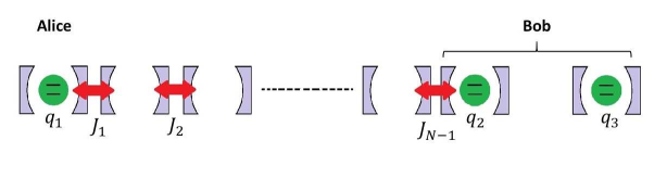
Figure 1: Schematic of coupled cavity array whose end cavities contain one atom in each. Atoms $q_{1}$ and $q_{2}$ are accessible by Alice and Bob respectively. Bob has an additional cavity with an atom $q_{3}$, which are not connected to each other as well as not coupled to the array.

A basic requirement for realizing quantum dense coding in our system is perfect transfer of a quanta between the qubits $q_{1}$ and $q_{2}$. If the qubit $q_{1}$ is in the excited state, and rest of the cavities and qubits are in their respective ground state, then the evolved state under the Hamiltonian $H$ is (for derivation refer the Appendix. A)

$$e^{-iHt}\ket{e}_{1}\ket{\text{vac}}\ket{g}_{2}\ket{g}_{3}=e^{-i\omega t}$$

$$\times \left[(\cos Jt)^{N+1}\ket{e}_{1}\ket{\text{vac}}\ket{g}_{2}\ket{g}_{3}\right.\left.+\sum_{k=1}^{N}C_{k}\ket{g}_{1}\ket{k}\rangle\ket{g}_{2}\ket{g}_{3}\right.$$

$$\left.+(-i\sin Jt)^{N+1}\ket{g}_{1}\ket{\text{vac}}\ket{e}_{2}\ket{g}_{3}\right],$$ (3)

where

$$C_{k}=\sqrt{\frac{(N+1)!}{(N+1-k)!k!}}(\cos Jt)^{N+1-k}(-i\sin Jt)^{k}.$$ (4)

Here $\ket{\text{vac}}$ is the state that represents all the cavities are in vacuum. The state $\ket{k}\rangle$ represents the $k$th cavity is in a single photon state and the rest of the cavities are in vacuum. The probability of transferring a quanta from $q_{1}$ to $q_{2}$ is

$$P=(\sin Jt)^{2(N+1)}.$$ (5)

The probability $P$ becomes unity at time $t=\pi/2J$, which we denote as $T$. This is the minimum time required to transfer a quanta between qubits $q_{1}$ and $q_{2}$.

3 Quantum dense coding in the array

In this section, we describe the dense coding protocol in our physical model. We consider the initial state of the system as

$$\ket{\psi(0)}=\frac{1}{\sqrt{2}}[\ket{g}_{1}\ket{\text{vac}}\ket{g}_{2}\ket{g}_{3}+\ket{e}_{1}\ket{\text{vac}}\ket{g}_{2}\ket{e}_{3}],$$ (6)

where the qubits $q_{1}$ and $q_{3}$ are entangled. This state can be prepared experimentally via entanglement swapping [45, 46, 47]. In order to encode the two classical bits in a single qubit, Alice applies unitary operation on her qubit depending on the choice of the classical bits. Table 1 shows the choices of classical bits and the corresponding unitary operations to be applied on Alice’s qubit.

Table 1: Classical bits and unitary operations.

$(x,y)$	unitary operation on $q_{1}$
(0,0)	$I$
(1,0)	$\sigma_{z}$
(0,1)	$\sigma_{x}$
(1,1)	$\sigma_{z}$ and $\sigma_{x}$

The actions of unitary operators on the qubit $q_{1}$ are $\sigma_{z}\ket{e}_{1}=\ket{e}_{1}$, $\sigma_{z}\ket{g}_{1}=-\ket{g}_{1}$, $\sigma_{x}\ket{e}_{1}=\ket{g}_{1}$, $\sigma_{x}\ket{g}_{1}=\ket{e}_{1}$. Then, the initial state given in Eqn. 6 after the unitary operation becomes

$$\ket{\psi_{1}}=\frac{1}{\sqrt{2}}[\ket{g}_{1}\ket{\text{vac}}\ket{g}_{2}\ket{g}_{3}+\ket{e}_{1}\ket{\text{vac}}\ket{g}_{2}\ket{e}_{3}],$$ (7a)

$$\ket{\psi_{2}}=\frac{1}{\sqrt{2}}[\ket{e}_{1}\ket{\text{vac}}\ket{g}_{2}\ket{e}_{3}-\ket{g}_{1}\ket{\text{vac}}\ket{g}_{2}\ket{g}_{3}],$$ (7b)

$$\ket{\psi_{3}}=\frac{1}{\sqrt{2}}[\ket{e}_{1}\ket{\text{vac}}\ket{g}_{2}\ket{g}_{3}+\ket{g}_{1}\ket{\text{vac}}\ket{g}_{2}\ket{e}_{3}],$$ (7c)

$$\ket{\psi_{4}}=\frac{1}{\sqrt{2}}[\ket{g}_{1}\ket{\text{vac}}\ket{g}_{2}\ket{e}_{3}-\ket{e}_{1}\ket{\text{vac}}\ket{g}_{2}\ket{g}_{3}],$$ (7d)

where $\ket{\psi_{1}}=I\ket{\psi(0)}$, $\ket{\psi_{2}}=\sigma_{z}\ket{\psi(0)}$, $\ket{\psi_{3}}=\sigma_{x}\ket{\psi(0)}$, $\ket{\psi_{4}}=\sigma_{x}\sigma_{z}\ket{\psi(0)}$. Now, Alice allows the qubit $q_{1}$ to interact with the cavity array. Then, the above states evolve under the Hamiltonian $H$ as

$$\ket{\psi_{1}(t)}=e^{-iHt}\ket{\psi_{1}}=\frac{1}{\sqrt{2}}\left[\ket{g}_{1}\ket{\text{vac}}\ket{g}_{2}\ket{g}_{3}\right.$$

$$+e^{-i\omega_{q3}t}e^{-i\omega t}\left[(\cos Jt)^{N+1}\ket{e}_{1}\ket{\text{vac}}\ket{g}_{2}\ket{e}_{3}\right.$$

$$\left.+\sum_{k=1}^{N}C_{k}\ket{g}_{1}\ket{k}\rangle\ket{g}_{2}\ket{e}_{3}\right.$$

$$\left.\left.+(-i\sin Jt)^{N+1}\ket{g}_{1}\ket{\text{vac}}\ket{e}_{2}\ket{e}_{3}\right]\right],$$ (8a)

$$\ket{\psi_{2}(t)}=e^{-iHt}\ket{\psi_{2}}=\frac{1}{\sqrt{2}}\left[-\ket{g}_{1}\ket{\text{vac}}\ket{g}_{2}\ket{g}_{3}\right.$$

$$+e^{-i\omega_{q3}t}e^{-i\omega t}\left[(\cos Jt)^{N+1}\ket{e}_{1}\ket{\text{vac}}\ket{g}_{2}\ket{e}_{3}\right.$$

$$\left.+\sum_{k=1}^{N}C_{k}\ket{g}_{1}\ket{k}\rangle\ket{g}_{2}\ket{e}_{3}\right.$$

$$\left.\left.+(-i\sin Jt)^{N+1}\ket{g}_{1}\ket{\text{vac}}\ket{e}_{2}\ket{e}_{3}\right]\right],$$ (8b)

$$\ket{\psi_{3}(t)}=e^{-iHt}\ket{\psi_{3}}=\frac{1}{\sqrt{2}}\left[\ket{g}_{1}\ket{\text{vac}}\ket{g}_{2}\ket{e}_{3}e^{-i\omega_{q3}t}\right.$$

$$+e^{-i\omega t}\left[(\cos Jt)^{N+1}\ket{e}_{1}\ket{\text{vac}}\ket{g}_{2}\ket{g}_{3}\right.$$

$$\left.+\sum_{k=1}^{N}C_{k}\ket{g}_{1}\ket{k}\rangle\ket{g}_{2}\ket{g}_{3}\right.$$

$$\left.\left.+(-i\sin Jt)^{N+1}\ket{g}_{1}\ket{\text{vac}}\ket{e}_{2}\ket{g}_{3}\right]\right],$$ (8c)

$$\ket{\psi_{4}(t)}=e^{-iHt}\ket{\psi_{4}}=\frac{1}{\sqrt{2}}\left[\ket{g}_{1}\ket{\text{vac}}\ket{g}_{2}\ket{e}_{3}e^{-i\omega_{q3}t}\right.$$

$$-e^{-i\omega t}\left[(\cos Jt)^{N+1}\ket{e}_{1}\ket{\text{vac}}\ket{g}_{2}\ket{g}_{3}\right.$$

$$\left.+\sum_{k=1}^{N}C_{k}\ket{g}_{1}\ket{k}\rangle\ket{g}_{2}\ket{g}_{3}\right.$$

$$\left.\left.+(-i\sin Jt)^{N+1}\ket{g}_{1}\ket{\text{vac}}\ket{e}_{2}\ket{g}_{3}\right]\right].$$ (8d)

The expression for $C_{k}$ is given in Eqn. 4. We set $\omega/J=4n-(N+1)$ and $\omega_{q3}/J=4m$ ($n$ and $m$ are two integers) for subsequent discussion. Then the evolved states at the time $T=\pi/2J$ are

$$\ket{\psi_{1}(T)}=\frac{1}{\sqrt{2}}[\ket{g}_{1}\ket{\text{vac}}\ket{g}_{2}\ket{g}_{3}+\ket{g}_{1}\ket{\text{vac}}\ket{e}_{2}\ket{e}_{3}],$$ (9a)

$$\ket{\psi_{2}(T)}=\frac{1}{\sqrt{2}}[\ket{g}_{1}\ket{\text{vac}}\ket{e}_{2}\ket{e}_{3}-\ket{g}_{1}\ket{\text{vac}}\ket{g}_{2}\ket{g}_{3}],$$ (9b)

$$\ket{\psi_{3}(T)}=\frac{1}{\sqrt{2}}[\ket{g}_{1}\ket{\text{vac}}\ket{e}_{2}\ket{g}_{3}+\ket{g}_{1}\ket{\text{vac}}\ket{g}_{2}\ket{e}_{3}],$$ (9c)

$$\ket{\psi_{4}(T)}=\frac{1}{\sqrt{2}}[\ket{g}_{1}\ket{\text{vac}}\ket{g}_{2}\ket{e}_{3}-\ket{g}_{1}\ket{\text{vac}}\ket{e}_{2}\ket{g}_{3}].$$ (9d)

It is to be noted that the qubits $q_{2}$ and $q_{3}$ become entangled in all these cases. In other words, entanglement between the qubits $q_{1}$ and $q_{3}$ was swapped to $q_{2}$ and $q_{3}$. The time $T=\pi/2J$ is the minimum time to transfer the information (swap the entanglement) and at this time Bob has to decouple qubit $q_{2}$ from the array. To decode the information, Bob applies a CNOT operation on his qubits $q_{2}$ and $q_{3}$. The CNOT operation [49, 50, 51] transforms the basis states as $U_{CNOT}\ket{g}_{2}\ket{g}_{3}=\ket{g}_{2}\ket{g}_{3}$, $U_{CNOT}\ket{g}_{2}\ket{e}_{3}=\ket{g}_{2}\ket{e}_{3}$, $U_{CNOT}\ket{e}_{2}\ket{g}_{3}=\ket{e}_{2}\ket{e}_{3}$ and $U_{CNOT}\ket{e}_{2}\ket{e}_{3}=\ket{e}_{2}\ket{g}_{3}$. The CNOT operation essentially disentangles qubits $q_{2}$ and $q_{3}$ [51]. After the CNOT operation, Bob applies a Hadamard operation on qubit $q_{2}$. The Hadamard operation [52] transforms the states as $U_{H}(\ket{g}_{2}+\ket{e}_{2})/\sqrt{2}=\ket{g}_{2}$ and $U_{H}(\ket{g}_{2}-\ket{e}_{2})/\sqrt{2}=\ket{e}_{2}$. After the CNOT and Hadamard operations, the states given in Eqns. (9a-9d) become $\ket{g}_{2}\ket{g}_{3}$, $\ket{e}_{2}\ket{g}_{3}$, $\ket{g}_{2}\ket{e}_{3}$ and $\ket{e}_{2}\ket{e}_{3}$ respectively. Now, by mapping the states $\ket{g}\rightarrow 0$ and $\ket{e}\rightarrow 1$, Bob recovers the classical bits.

It is to be noted that the probability of transferring the information depends on the evolution of the states from Eqns. (7a-7d) to Eqns. (9a-9d). Hence, the fidelity of information transfer is

$$F_{i}=|\bra{\psi_{i}(T)}e^{-iHt}\ket{\psi_{i}}|^{2}.~{}~{}~{}(i=1,2,3,4)$$ (10)

Fidelities are shown in Fig. 2. It is seen that fidelities are unity at $T=\pi/2J$. We have chosen $\omega/J=4n-(N+1)$ and $\omega_{q3}/J=4m$ with $n=2500,m=2500$ and $N=4$. Hence, the choice of coupling strengths given in Eqn. 2 ensures perfect transfer of information. It is seen that $F_{1}=F_{2}$ and $F_{3}=F_{4}$.

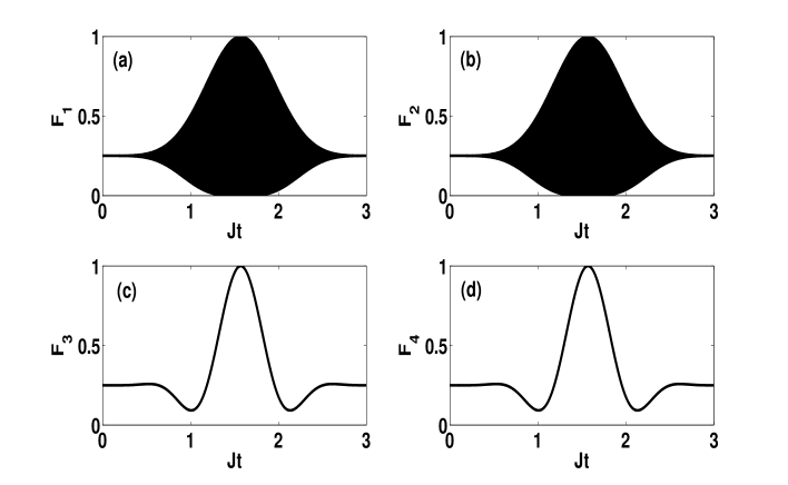
Figure 2: Fidelities $F_{1},F_{2},F_{3}$ and $F_{4}$ as a function of $Jt$. We choose $\omega/J=9.995\times 10^{3}$, $\omega_{q3}/J=10^{4}$ and $N=4$. All the coupling strengths satisfy the relation given in Eqn. 2.

4 Results and discussion

In this section, we will discuss the quantum dense coding protocol by considering experimentally achievable parameters. As dissipation is unavoidable, we include the dissipation in the system. Loss of photons may occur via spontaneous emission or leakage through the cavity walls. The effect of dissipation on the fidelity of information transfer is studied by analyzing the master equation. The master equation that includes the dissipation in the system is [53]

$$\frac{\partial\rho}{\partial t}=\frac{-i}{\hbar}[H,\rho]+\frac{k}{2}\sum_{j=1}^{N+1}\mathcal{L}[a_{j}]\rho+\frac{\gamma}{2}\sum_{j=1}^{3}\mathcal{L}[(\sigma_{-})_{qj}]\rho,$$ (11)

where $\mathcal{L}[o]\rho=2o\rho o^{\dagger}-o^{\dagger}o\rho-\rho o^{\dagger}o$ is the Lindblad superoperator [54], and $k$ and $\gamma$ are the dissipation rates of cavities and atoms respectively. In order to minimize the effect of dissipation on fidelities, a cavity array with high quality factors ($Q$-factors) is necessary. High $Q$ value implies that the photon life time inside the cavity is large. Recently, photonic crystal cavities with large $Q$ factor have been fabricated and the order of $Q$-factor was $\sim 10^{6}$ [55, 56, 57]. Another factor that can minimize the effect of dissipation is the coupling strength. If the cavities are highly coupled then the time for the information transfer will be small, as a result the effect of dissipation will be small. Highly coupled cavities are already been realized in the context of photonic crystal cavities whose coupling strengths are of the order of $\sim$ THz [58]. Hence, an array of photonic crystal cavities may be a suitable physical system for realizing this protocol. Another platform which is suitable for realizing the quantum dense coding protocol is a superconducting resonator array. It is possible to fabricate superconducting resonators with $Q$-factors larger than $10^{6}$ [59].

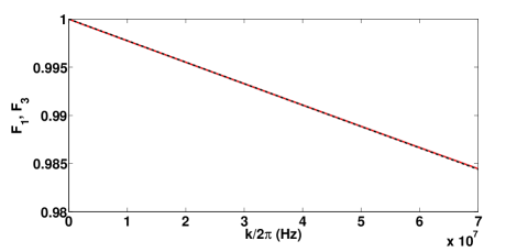
Figure 3: Fidelities $F_{1}$ (continuous) and $F_{3}$ (dashed) at time $T=\pi/2J$ are shown as a function of cavity decay rate $k/2\pi$. We choose $(\omega/2\pi,\omega_{q3}/2\pi)=(6.92,7)$THz, $(J/2\pi,g/2\pi)=(7,23.21)$GHz, $\gamma/2\pi=3.5$ MHz and $N=10$.

For the purpose of demonstration of quantum dense coding, we plot $F_{1}$ and $F_{3}$ as a function of $k/2\pi$ in Fig. 3 by setting $(\omega/2\pi,\omega_{q3}/2\pi)=(6.92,7)$THz, $(J/2\pi,g/2\pi)=(7,23.21)$GHz and the atomic decay rate $\gamma/2\pi=3.5$ MHz. These values are easily achievable in photonic crystal cavities [58, 60, 61, 62, 63]. As seen from the figure, the fidelity of information transfer is more than $0.98$ even for large dissipation rate. We have taken $N=10$. The time for information transfer is $\pi/2J\sim 0.22$ns, which is much smaller than the cavity decay time $2\pi/k\sim 14$ns for $k/2\pi=70$ MHz. In the case of superconducting resonators, we set $J/2\pi=1.9$ MHz, $\omega/2\pi=1.88$ GHz, $\omega_{q3}=1.9$ GHz and the coupling between the resonator and superconducting qubit is taken to be $g/2\pi=6.3$ MHz [64, 65, 66]. The decay parameters are chosen to be $k/2\pi=1.8$ kHz and $\gamma/2\pi=1$ kHz. The number of resonators in the array is $N=10$. Using these values, the fidelity of information transfer is found to be $0.992$. In this case, the time for information transfer is $0.82\mu$s while the resonator relaxation time is $0.87$ms.

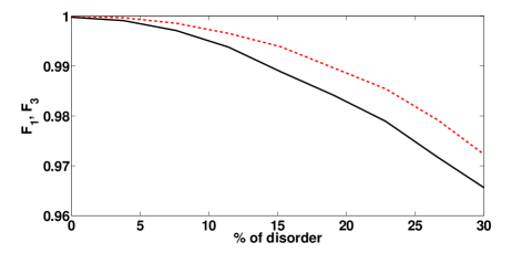
Figure 4: Fidelities $F_{1}$ (continuous) and $F_{3}$ (dashed) at time $T=\pi/2J$ are shown as a function of percentage of disorder. We choose $(\omega/2\pi,\omega_{q3}/2\pi)=(6.92,7)$THz, $(J/2\pi,g/2\pi)=(7,23.21)$GHz and $N=10$.

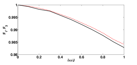
Figure 5: Fidelities $F_{1}$ (continuous) and $F_{3}$ (dashed) at time $T=\pi/2J$ are shown as a function $\delta\omega/J$. We choose $(\omega/2\pi,\omega_{q3}/2\pi)=(6.92,7)$THz, $(J/2\pi,g/2\pi)=(7,23.21)$GHz and $N=10$.

In a realistic situation, apart from dissipation, another factor that can reduce the fidelity of transfer is disorder in the system. As seen in the previous section, a suitable combination of coupling strengths as is given in Eqn. 2 provides perfect transfer of information if the cavities and atoms are in resonance. However, in an experimental situation, precise control of coupling strengths and resonance frequencies may not be possible. Hence, we consider small disorder in the coupling strengths as well as in the resonance frequencies. We first consider the effect of coupling disorder. Let the coupling strength $J_{k}$ fluctuates around $J_{k}\pm\frac{\delta J}{2}$ such that $\delta J$ is the width of the disorder. Here $J_{k}$ is the coupling strength between the $k$th and $(k+1)$th cavities. So, $J_{k}$ has to be chosen randomly between $J_{k}-\frac{\delta J}{2}$ and $J_{k}+\frac{\delta J}{2}$. Also, we assume that the atom-cavity coupling strength $g$ fluctuates within a range $\delta g$. For simplicity, we take $\delta g=\delta J$. For a given set of coupling strengths that are chosen randomly from within the aforementioned interval, we calculate the fidelity of transfer at $T=\pi/2J$ and take average over all the sets of coupling strengths. We take 1000 realizations, i.e., 1000 sets of coupling strengths are chosen randomly from within the interval. Fig. 4 shows average fidelities $F_{1}$ and $F_{3}$ as a function of the percentage of the disorder. Percentage of the disorder is defined as $\frac{\delta J}{\langle J\rangle}\times 100$, where $\langle J\rangle=(\sum_{k=1}^{N-1}J_{k})/(N-1)$ is the average of all the coupling strengths. We set $J/2\pi=7$ GHz and the width of the disorder $\delta J$ is varied up to $30\%$ of $\langle J\rangle$. As can be seen in figure, the fidelity is more than 0.95 even in the presence of large disorder in coupling strengths. As, $F_{1}=F_{2}$ and $F_{3}=F_{4}$, we only plot $F_{1}$ and $F_{3}$ in the figure.

Now, we consider the disorder in the resonance frequencies. Let the cavity resonance frequencies are fluctuating around $\omega\pm\delta\omega/2$. Hence, the width of the disorder is $\delta\omega$. We plot the average fidelities $F_{1}$ and $F_{3}$ in Fig. 5 as a function of $\delta\omega/J$. The average is taken over 1000 realizations, i.e., the set of resonance frequencies are chosen 1000 times from within the aforementioned interval. As can be seen in the figure, the fidelity of information transfer is high even in the presence of large detuning between the cavities. Hence, the scheme is robust in the presence of experimental imperfections like coupling disorder and frequency disorder.

5 Summary

Quantum dense coding is one of the most important protocols for realizing quantum communication, where two bits of classical information can be transferred by sending only one quantum bit. We have proposed an experimentally realizable quantum dense coding protocol via entanglement swapping in a cavity array containing certain number of atoms. By suitably choosing the inter-cavity coupling strengths and the atom-cavity coupling strengths, the fidelity for transfer of the information from the sender to receiver is high even in the presence of dissipation and disorder. It is possible to transfer the information with fidelity more than $0.95$ in the context of photonic crystal cavities and superconducting resonators. Fidelities can be improved further by improving the quality factor of the cavities and increasing the coupling strengths. Our scheme is also robust against experimental imperfections such as disorder in the coupling strengths and resonance frequencies. Recent progress in the fabrication of high quality cavities suggests that our scheme may be a good candidate for realizing quantum dense coding protocol in the context of cavity QED. The proposed scheme can also be implemented in the context of spin chains, Josephson junction array, quantum dot array, optomechanical cavity array, etc. We believe that our scheme will be of use for realizing future quantum communication.

Appendix A: Time evolution of the state

The Hamiltonian given in Eqn. 2 in interaction picture is

$$H_{\text{int}} =\sum_{k=1}^{N-1}\sqrt{(k+1)(N+1-k)}J(a_{k}^{\dagger}a_{k+1}+a_{k}a_{k+1}^{\dagger})$$

$$+ \sqrt{N+1}J[a_{1}^{\dagger}(\sigma_{-})_{q1}+a_{1}(\sigma_{+})_{q1}+a_{N}^{\dagger}(\sigma_{-})_{q2}+a_{N}(\sigma_{+})_{q2}].$$ (A1)

The matrix form of the interaction Hamiltonian in the basis $\{\ket{e}_{1}\ket{\text{vac}}\ket{g}_{2}\}$,$\{\ket{g}_{1}\ket{1}\rangle\ket{g}_{2}\}$, $\{\ket{g}_{1}\ket{2}\rangle\ket{g}_{2}\}$,……, $\{\ket{g}_{1}\ket{N}\rangle\ket{g}_{2}\}$, $\{\ket{g}_{1}\ket{\text{vac}}\ket{e}_{2}\}$ is

$$H_{\text{int}}=J\left[\begin{array}[]{ccccc}0&\sqrt{N+1}&0&\cdots&0\\ \sqrt{N+1}&0&\sqrt{2N}&\cdots&0\\ 0&\sqrt{2N}&0&\cdots&0\\ \vdots&\vdots&\vdots&\cdots&\sqrt{N+1}\\ 0&0&0&\sqrt{N+1}&0\end{array}\right].$$ (A7)

One can see that this Hamiltonian is equivalent to the Hamiltonian corresponding to two coupled cavities having $(N+1)$ quanta. The Hamiltonian for the two coupled cavities is $\tilde{H}_{\text{int}}=J(\tilde{a}_{1}^{\dagger}\tilde{a}_{2}+\tilde{a}_{1}\tilde{a}^{\dagger}_{2})$. Also, the basis states of both the systems can be mapped to each other, i.e., $\{\ket{e}_{1}\ket{\text{vac}}\ket{g}_{2}\}\rightarrow\ket{N+1,0}$, $\{\ket{g}_{1}\ket{1}\rangle\ket{g}_{2}\}\rightarrow\ket{N,1}$, $\{\ket{g}_{1}\ket{2}\rangle\ket{g}_{2}\}\rightarrow\ket{N-1,2}$,……, $\{\ket{g}_{1}\ket{N}\rangle\ket{g}_{2}\}\rightarrow\ket{1,N}$ and $\{\ket{g}_{1}\ket{\text{vac}}\ket{e}_{2}\}\rightarrow\ket{0,N+1}$. Similar kind duality has already been used in the context of cavity array [16].

As the Hamiltonians are equivalent, the time evolution of the states is also equivalent. Evolution of the state $\ket{N+1-n,n}$ under the interaction Hamiltonian $\tilde{H}_{int}$ is

$$e^{-i\tilde{H}_{\text{int}}t}\ket{N+1-n,n}= e^{-i\tilde{H}_{\text{int}}t}\frac{\tilde{a}_{1}^{\dagger N+1-n}\tilde{a}_{2}^{\dagger n}}{\sqrt{(N+1-n)!n!}}\ket{0,0}.$$ (A8)

Using Baker-Hausdorf lemma [67], we obtained $e^{-i\tilde{H}_{\text{int}}t}\tilde{a}_{1}e^{-i\tilde{H}_{\text{int}}t}=\tilde{a}_{1}\cos Jt+i\tilde{a}_{2}\sin Jt$, $e^{-i\tilde{H}_{\text{int}}t}\tilde{a}_{2}e^{-i\tilde{H}_{\text{int}}t}=\tilde{a}_{2}\cos Jt+i\tilde{a}_{1}\sin Jt$. Using these relations, Eqn. A8 becomes

$$e^{-i\tilde{H}_{\text{int}}t}\ket{N+1-n,n}=$$

$$\frac{(\tilde{a}_{1}^{\dagger}\cos Jt-i\tilde{a}_{2}^{\dagger}\sin Jt)^{N+1-n}(\tilde{a}_{2}^{\dagger}\cos Jt-i\tilde{a}_{1}^{\dagger}\sin Jt)^{n}}{\sqrt{(N+1-n)!n!}}\ket{0,0}.$$ (A9)

Using binomial expansion, we arrived at

$$e^{-i\tilde{H}_{\text{int}}t}\ket{N+1-n,n}=$$

$$\sum_{k=0}^{N+1-n}\sum_{l=0}^{n}~{}^{N+1-n}C_{k}~{}^{n}C_{l}(\cos Jt)^{N+1-(k+l)}(-i\sin Jt)^{k+l}$$

$$\frac{\sqrt{(N+1-(n+k-l))!(n+k-l)!}}{\sqrt{(N+1-n)!n!}}\ket{N+1-(n+k-l),n+k-l}.$$

For $n=0$, the evolved state becomes

$$e^{-i\tilde{H}_{\text{int}}t}\ket{N+1,0}= \sum_{k=0}^{N+1}C_{k}(\cos Jt)^{N+1-k}(-i\sin Jt)^{k}\ket{N+1-k,k},$$

where the expression for $C_{k}$ is given in Eqn. 4. Equivalently, in the cavity array, the evolved state becomes

$$e^{-iH_{\text{int}}t}\ket{e}_{1}\ket{\text{vac}}\ket{g}_{2}=\left[(\cos Jt)^{N+1}\ket{e}_{1}\ket{\text{vac}}\ket{g}_{2}\right.$$

$$\left.+\sum_{k=1}^{N}C_{k}\ket{g}_{1}\ket{k}\rangle\ket{g}_{2}\right.\left.+(-i\sin Jt)^{N+1}\ket{g}_{1}\ket{\text{vac}}\ket{e}_{2}\right].$$ (A10)

References

References

- [1] Bennett C H and Wiesner S J 1992 Phys. Rev. Lett. 69(20) 2881–2884 URL https://link.aps.org/doi/10.1103/PhysRevLett.69.2881
- [2] Mattle K, Weinfurter H, Kwiat P G and Zeilinger A 1996 Phys. Rev. Lett. 76(25) 4656–4659 URL https://link.aps.org/doi/10.1103/PhysRevLett.76.4656
- [3] Ban M 1999 Journal of Optics B: Quantum and Semiclassical Optics 1 L9–L11
- [4] Qiu L, Wang A M and Ma X S 2007 Physica A: Statistical Mechanics and its Applications 383 325 – 330 ISSN 0378-4371
- [5] Simayi S, Abulizi A, Yaermaimaiti M, Cai J T and Qiao P P 2011 Chinese Physics B 20 050305
- [6] Xu H Y and Yang G H 2017 International Journal of Theoretical Physics 56 2803–2810 ISSN 1572-9575 URL https://doi.org/10.1007/s10773-017-3445-0
- [7] Huang H 2009 International Journal of Theoretical Physics 48 3491 ISSN 1572-9575 URL https://doi.org/10.1007/s10773-009-0153-4
- [8] Lin X M, Zhou Z W, Xue P, Gu Y J and Guo G C 2003 Physics Letters A 313 351 – 355 ISSN 0375-9601
- [9] Ye L and Guo G C 2005 Phys. Rev. A 71(3) 034304 URL https://link.aps.org/doi/10.1103/PhysRevA.71.034304
- [10] Xue Z Y, min Yi Y and liang Cao Z 2006 Journal of Modern Optics 53 2725–2732
- [11] Chun-Xia J and Zhao-Hui P 2008 Communications in Theoretical Physics 50 1113–1116
- [12] Juan H, Liu Y and Zhi-Xiang N 2008 Chinese Physics B 17 1597–1600
- [13] Nie Y y, Li Y h, Wang X p and Sang M h 2013 Quantum Information Processing 12 1851–1857 ISSN 1573-1332 URL https://doi.org/10.1007/s11128-012-0499-z
- [14] Reiserer A and Rempe G 2015 Rev. Mod. Phys. 87(4) 1379–1418
- [15] Wu Q and Yang M 2008 International Journal of Theoretical Physics 47 3139–3143 ISSN 1572-9575
- [16] Meher N, Sivakumar S and Panigrahi P K 2017 Scientific Reports 7 9251– ISSN 2045-2322
- [17] Almeida G M A, Ciccarello F, Apollaro T J G and Souza A M C 2016 Phys. Rev. A 93(3) 032310
- [18] Liu Y and Zhou D L 2015 New Journal of Physics 17 013032
- [19] Yung M H and Bose S 2005 Phys. Rev. A 71(3) 032310
- [20] Meher N 2019 Journal of Physics B: Atomic, Molecular and Optical Physics 52 205502
- [21] de Moraes Neto G D, Andrade F M, Montenegro V and Bose S 2016 Phys. Rev. A 93(6) 062339
- [22] Hua M, Tao M J and Deng F G 2016 Scientific Reports 6 22037–
- [23] Meher N 2020 International Journal of Theoretical Physics 59 218–228 ISSN 1572-9575 URL https://doi.org/10.1007/s10773-019-04314-1
- [24] Leonski W and Miranowicz A 2004 Journal of Optics B: Quantum and Semiclassical Optics 6 S37
- [25] Liew T C H and Savona V 2013 New Journal of Physics 15 025015
- [26] Browne D E and Plenio M B 2003 Phys. Rev. A 67(1) 012325
- [27] Miry S R, Tavassoly M K and Roknizadeh R 2015 Quantum Information Processing 14 593–606 ISSN 1573-1332
- [28] Yurke B and Stoler D 1986 Phys. Rev. Lett. 57(1) 13–16
- [29] Rojan K, Reich D M, Dotsenko I, Raimond J M, Koch C P and Morigi G 2014 Phys. Rev. A 90(2) 023824
- [30] Wei W and Guang-can G 1998 Acta Physica Sinica (Overseas Edition) 7 174
- [31] Wang Y, Wan J, Zou B, Zhang J and Zhu Y 2013 Journal of Physics: Conference Series 414 012001
- [32] Meher N and Sivakumar S 2018 Quantum Information Processing 17 233 ISSN 1573-1332
- [33] Meher N and Sivakumar S 2016 J. Opt. Soc. Am. B 33 1233–1241
- [34] Schmidt S, Gerace D, Houck A A, Blatter G and Türeci H E 2010 Phys. Rev. B 82(10) 100507
- [35] Asadian A, Manzano D, Tiersch M and Briegel H J 2013 Phys. Rev. E 87(1) 012109
- [36] Meher N and Sivakumar S 2020 J. Opt. Soc. Am. B 37 138–147 URL http://josab.osa.org/abstract.cfm?URI=josab-37-1-138
- [37] Xuereb A, Imparato A and Dantan A 2015 New Journal of Physics 17 055013
- [38] Imamoglu A, Schmidt H, Woods G and Deutsch M 1997 Phys. Rev. Lett. 79(8) 1467–1470
- [39] Birnbaum K M, Boca A, Miller R, Boozer A D, Northup T E and Kimble H J 2005 Nature 436 87–
- [40] Tang J, Geng W and Xu X 2015 Scientific Reports 5 9252–
- [41] Shen H Z, Zhou Y H and Yi X X 2015 Phys. Rev. A 91(6) 063808
- [42] Miranowicz A, Bajer J c v, Paprzycka M, Liu Y x, Zagoskin A M and Nori F 2014 Phys. Rev. A 90(3) 033831
- [43] Zhou L, Gong Z R, Liu Y x, Sun C P and Nori F 2008 Phys. Rev. Lett. 101(10) 100501
- [44] Qin W and Nori F 2016 Phys. Rev. A 93(3) 032337
- [45] Yang M, Zhao Y, Song W and Cao Z L 2005 Phys. Rev. A 71(4) 044302 URL https://link.aps.org/doi/10.1103/PhysRevA.71.044302
- [46] Ying-Qiao Z, Xing-Ri J and Shou Z 2005 Chinese Physics 14 1732–1735
- [47] Xiu L, Hong-Cai L, Xiu-Min L, Xing-Hua L and Rong-Can Y 2007 Chinese Physics 16 1209–1214
- [48] Joglekar Y N, Thompson C, Scott D D and Vemuri G 2013 The European Physical Journal Applied Physics 63
- [49] DiVincenzo D P 1995 Phys. Rev. A 51(2) 1015–1022
- [50] DiVincenzo D P 2000 Fortschritte der Physik 48 771–783
- [51] Barenco A, Deutsch D, Ekert A and Jozsa R 1995 Phys. Rev. Lett. 74(20) 4083–4086 URL https://link.aps.org/doi/10.1103/PhysRevLett.74.4083
- [52] DiVincenzo D P 1995 Science 270 255–261 ISSN 0036-8075 URL https://science.sciencemag.org/content/270/5234/255
- [53] Carmichael H J 1999 Statistical Methods in Quantum Optics 1: Master Equations and Fokker-Planck Equations (Springer)
- [54] Lindblad G 1976 Commun.Math. Phys. 48(2) 195452
- [55] Notomi M, Tanabe T, Shinya A, Kuramochi E, Taniyama H, Mitsugi S and Morita M 2007 Opt. Express 15 17458–17481
- [56] Notomi M, Kuramochi E and Tanabe T 2008 Nature Photonics 2 741–
- [57] Vasco J P and Savona V 2018 New Journal of Physics 20 075002
- [58] Majumdar A, Rundquist A, Bajcsy M, Dasika V D, Bank S R and Vučković J 2012 Phys. Rev. B 86(19) 195312
- [59] Kuhr S, Gleyzes S, Guerlin C, Bernu J, Hoff U B, Deleglise S, Osnaghi S, Brune M, Raimond J M, Haroche S, Jacques E, Bosland P and Visentin B 2007 Applied Physics Letters 90 164101
- [60] Majumdar A, Rundquist A, Bajcsy M and Vučković J 2012 Phys. Rev. B 86(4) 045315
- [61] Xiao Y F, Gao J, Zou X B, McMillan J F, Yang X, Chen Y L, Han Z F, Guo G C and Wong C W 2008 New Journal of Physics 10 123013
- [62] Tiecke T G, Thompson J D, de Leon N P, Liu L R, Vuletic V and Lukin M D 2014 Nature 508 241 URL https://doi.org/10.1038/nature13188
- [63] Du H, Zhang X, Chen G, Deng J, Chau F S and Zhou G 2016 Scientific Reports 6 24766
- [64] Ma S l, Xie J k, Li X k and Li F l 2019 Phys. Rev. A 99(4) 042317
- [65] Chen Q M, Liu Y x, Sun L and Wu R B 2018 Phys. Rev. A 98(4) 042328
- [66] Li H, Wang Y, Wei L, Zhou P, Wei Q, Cao C, Fang Y, Yu Y and Wu P 2013 Chinese Science Bulletin 58 2413–2417
- [67] Gerry C and Knight P 2004 Introductory Quantum Optics (Cambridge University Press) ISBN 052152735X