Dyakonov–Tamm surface waves featuring Dyakonov–Tamm–Voigt surface waves

Abstract

The propagation of Dyakonov–Tamm (DT) surface waves guided by the planar interface of two nondissipative materials ${\cal A}$ and ${\cal B}$ was investigated theoretically and numerically, via the corresponding canonical boundary-value problem. Material ${\cal A}$ is a homogeneous uniaxial dielectric material whose optic axis lies at an angle $\chi$ relative to the interface plane. Material ${\cal B}$ is an isotropic dielectric material that is periodically nonhomogeneous in the direction normal to the interface. The special case was considered in which the propagation matrix for material ${\cal A}$ is non-diagonalizable because the corresponding surface wave — named the Dyakonov–Tamm–Voigt (DTV) surface wave — has unusual localization characteristics. The decay of the DTV surface wave is given by the product of a linear function and an exponential function of distance from the interface in material ${\cal A}$; in contrast, the fields of conventional DT surface waves decay only exponentially with distance from the interface. Numerical studies revealed that multiple DT surface waves can exist for a fixed propagation direction in the interface plane, depending upon the constitutive parameters of materials ${\cal A}$ and ${\cal B}$. When regarded as functions of the angle of propagation in the interface plane, the multiple DT surface-wave solutions can be organized as continuous branches. A larger number of DT solution branches exist when the degree of anisotropy of material ${\cal A}$ is greater. If $\chi=0^{\circ}$ then a solitary DTV solution exists for a unique propagation direction on each DT branch solution. If $\chi>0^{\circ}$, then no DTV solutions exist. As the degree of nonhomogeneity of material ${\cal B}$ decreases, the number of DT solution branches decreases. For most propagation directions in the interface plane, no solutions exist in the limiting case wherein the degree of nonhomogeneity approaches zero; but one solution persists provided that the direction of propagation falls within the angular existence domain of the corresponding Dyakonov surface wave.

1 Introduction

Electromagnetic surface waves of different types can be guided by the planar interface of two dissimilar linear materials, depending upon the constitutive characteristics of the two partnering materials [1, 2]. For example, if one partnering material is an isotropic dielectric material and the other is an anisotropic dielectric material, with both materials being homogeneous, then the planar interface can guide the propagation of Dyakonov surface waves [3, 4, 5, 6, 7]. A different type of surface wave can propagate if one of the partnering materials is periodically nonhomogeneous in the direction normal to the interface. For example, if both partnering materials are dielectric materials with one being anisotropic and one (possibly the same one) being periodically nonhomogeneous, then the planar interface can guide the propagation of Dyakonov–Tamm (DT) surface waves [8, 9]. Both Dyakonov surface waves and DT surface waves can propagate without decay when dissipation is so small that it can be ignored in both partnering materials — a characteristics which makes these surface waves attractive for applications involving long-range optical communications [10, 11]. Unlike Dyakonov surface waves, DT surface waves typically propagate for a wide range of directions parallel to the interface plane. Also unlike Dyakonov surface waves in the absence of dissipation, multiple DT surface waves with different phase speeds and decay constants can propagate in a fixed direction parallel to the interface plane — a property which makes them attractive for optical-sensing applications [12].

All previous works on DT surface waves [8, 9, 13, 14, 15], including experimental observations [16, 17], have focused on the planar interface of a homogeneous isotropic material and a periodically nonhomogeneous anisotropic material. In contrast, here we consider the planar interface of a homogeneous anisotropic material and a periodically nonhomogeneous isotropic material. This case provides a convenient means of studying Dyakonov–Tamm–Voigt (DTV) surface waves, which have not been described previously.

As elaborated upon in the ensuing sections, a DTV surface wave can exist when a propagation matrix for the anisotropic partnering material is non-diagonalizable. The localization of DTV surface waves is fundamentally different from the localization of DT surface waves. Specifically, as the distance from the planar interface increases in the anisotropic partnering material, the amplitude of a DTV surface wave decays in a combined exponential–linear manner, whereas the amplitudes of DT surface waves decay only in an exponential manner. Also, a DTV surface wave propagates in only a single direction in each quadrant of the interface plane; in contrast, DT surface waves propagate for a range of directions in each quadrant of the interface plane.

The fields of the DTV surface wave in the anisotropic partnering material have certain characteristics in common with the fields associated with a singular form of planewave propagation called Voigt-wave propagation [18, 19, 20]. A Voigt wave can exist when the planewave propagation matrix is non-diagonalizable [21, 22, 23, 24]. Unlike conventional plane waves [25, 26], the decay of Voigt waves is characterized by the product of an exponential function of the propagation distance and a linear function of the propagation distance.

In this paper the theory underpinning the propagation of DT and DTV surface waves is presented for the canonical boundary-value problem of surface-wave propagation [2] guided by the planar interface of a homogeneous uniaxial dielectric material and a periodically nonhomogeneous isotropic dielectric material. The theory is illustrated by means of representative numerical calculations, based on realistic values for the constitutive parameters of the partnering materials.

The following notation is adopted: The permittivity and permeability of free space are denoted by $\varepsilon_{\scriptscriptstyle 0}$ and $\mu_{\scriptscriptstyle 0}$, respectively. The free-space wavelength is written as $\lambda_{\scriptscriptstyle 0}=2\pi/k_{\scriptscriptstyle 0}$ with $k_{\scriptscriptstyle 0}=\omega\sqrt{\varepsilon_{\scriptscriptstyle 0}\mu_{\scriptscriptstyle 0}}$ being the free-space wavenumber and $\omega$ being the angular frequency. An $\exp(-i\omega t)$ dependence on time $t$ is implicit, with $i=\sqrt{-1}$. The real and imaginary parts of complex-valued quantities are delivered by the operators $\mbox{Re}\left\{\mbox{ \tiny{${}^{\bullet}$} }\right\}$ and $\mbox{Im}\left\{\mbox{ \tiny{${}^{\bullet}$} }\right\}$, respectively. Single underlining denotes a 3-vector and $\left\{\hat{\underline{u}}_{x},\hat{\underline{u}}_{y},\hat{\underline{u}}_{z}\right\}$ is the triad of unit vectors aligned with the Cartesian axes. Dyadics are double underlined [25]. Square brackets enclose matrixes and column vectors. The superscript ^T denotes the transpose. The complex conjugate is denoted by an asterisk.

2 Theory

2.1 Preliminaries

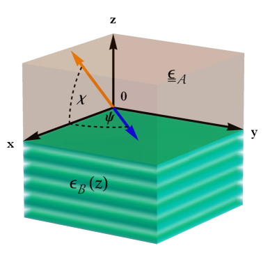
Figure 1: Schematic representation of the canonical boundary-value problem solved. The optic axis of material ${\cal A}$ lies in the $xz$ plane, oriented at the angle $\chi$ relative to $x$-axis. Surface waves propagate parallel to the interface $z=0$, at the angle $\psi$ relative to the $x$-axis.

In the canonical boundary-value problem, material ${\cal A}$ occupies the half-space $z>0$ and material ${\cal B}$ the half-space $z<0$, as represented schematically in Fig. 1. Whereas material ${\cal A}$ is anisotropic and homogeneous, material ${\cal B}$ is isotropic and periodically nonhomogeneous along the $z$ axis. Both materials are dielectric, and possess neither magnetic nor magnetoelectric properties different from free space [27, 28, 26].

The relative permittivity dyadic of material ${\cal A}$ is given as [25]

$$\underline{\underline{\varepsilon}}_{\cal A}=\underline{\underline{S}}_{y}(\chi)\mbox{ \tiny{${}^{\bullet}$} }\left[{\varepsilon}_{\cal A}^{t}\hat{\underline{u}}_{x}\,\hat{\underline{u}}_{x}+{\varepsilon}_{\cal A}^{s}\left(\hat{\underline{u}}_{y}\,\hat{\underline{u}}_{y}+\hat{\underline{u}}_{z}\,\hat{\underline{u}}_{z}\right)\right]\mbox{ \tiny{${}^{\bullet}$} }\underline{\underline{S}}_{y}^{T}(\chi),$$ (1)

wherein the rotation dyadic

$$\underline{\underline{S}}_{y}(\chi)=\hat{\underline{u}}_{y}\,\hat{\underline{u}}_{y}+\left(\hat{\underline{u}}_{x}\,\hat{\underline{u}}_{x}+\hat{\underline{u}}_{z}\,\hat{\underline{u}}_{z}\right)\cos\chi+\left(\hat{\underline{u}}_{z}\,\hat{\underline{u}}_{x}-\hat{\underline{u}}_{x}\,\hat{\underline{u}}_{z}\right)\sin\chi.$$ (2)

Thus, the optic axis of material ${\cal A}$ lies wholly in the $xz$ plane at an angle $\chi$ with respect to the $x$ axis. Although the relative permittivity parameters $\varepsilon^{s}_{\cal A}$ and $\varepsilon^{t}_{\cal A}$ are generally complex valued, in the proceeding numerical studies we have confined ourselves to $\varepsilon^{s}_{\cal A}\in\mathbb{R}$ and $\varepsilon^{t}_{\cal A}\in\mathbb{R}$, as is commonplace in crystal optics [29].

The relative permittivity dyadic of material ${\cal B}$ is specified as $\underline{\underline{\varepsilon}}_{\cal B}(z)=\varepsilon_{\cal B}(z)\underline{\underline{I}}$, where

$$\varepsilon_{\cal B}(z)=\left[\frac{n_{1}+n_{2}}{2}+\gamma\frac{n_{1}-n_{2}}{2}\sin\left(\frac{\pi z}{\Omega}\right)\right]^{2}\,,$$ (3)

and $\underline{\underline{I}}=\hat{\underline{u}}_{x}\,\hat{\underline{u}}_{x}+\hat{\underline{u}}_{y}\,\hat{\underline{u}}_{y}+\hat{\underline{u}}_{z}\,\hat{\underline{u}}_{z}$ is the 3$\times$3 identity dyadic [25]. In Eq. (3), the parameter $\Omega>0$ is the half-period of the periodic variation in dielectric properties along the negative $z$ axis, while $\gamma>0$ is a scaling parameter for the amplitude of this periodic variation. The parameter $\gamma$ can be considered to be the degree of nonhomogeneity when $\Omega$ is finite. We take the refractive indexes $n_{1}$ and $n_{2}$ to be real and positive, as is commonplace in the literature on rugate filters [30, 31].

The electromagnetic field phasors for surface-wave propagation are expressed everywhere as [2]

$$\left.\begin{array}[]{l}\underline{E}(\underline{r})=\left[e_{x}(z)\hat{\underline{u}}_{x}+e_{y}(z)\hat{\underline{u}}_{y}+e_{z}(z)\hat{\underline{u}}_{z}\right]\,\exp\left[iq\left(x\cos\psi+y\sin\psi\right)\right]\\[4.0pt] \underline{H}(\underline{r})=\left[h_{x}(z)\hat{\underline{u}}_{x}+h_{y}(z)\hat{\underline{u}}_{y}+h_{z}(z)\hat{\underline{u}}_{z}\right]\,\exp\left[iq\left(x\cos\psi+y\sin\psi\right)\right]\end{array}\right\}\,,\>\>\>-\infty<z<+\infty,$$ (4)

with ${q}$ being the surface wavenumber. The angle $\psi\in\left[0,2\pi\right)$ specifies the direction of propagation in the $xy$ plane, relative to the $x$ axis. The phasor representations (4), when combined with the source-free Faraday and Ampére–Maxwell equations, deliver the 4$\times$4 matrix ordinary differential equations [32, 33]

$$\frac{d}{dz}\left[\underline{f}(z)\right]=\left\{\begin{array}[]{l}i\left[\underline{\underline{P}}_{\cal A}\right]\mbox{ \tiny{${}^{\bullet}$} }\left[\underline{f}(z)\right]\,,\qquad z>0\vspace{8pt}\\ i\left[\underline{\underline{P}}_{\cal B}(z)\right]\mbox{ \tiny{${}^{\bullet}$} }\left[\underline{f}(z)\right]\,,\qquad z<0\end{array},\right.$$ (5)

wherein the column 4-vector

$$\left[\underline{f}(z)\right]=\left[\begin{array}[]{c}e_{x}(z),\quad e_{y}(z),\quad h_{x}(z),\quad h_{y}(z)\end{array}\right]^{T},$$ (6)

and the 4$\times$4 propagation matrixes $\left[\underline{\underline{P}}_{\cal A}\right]$ and $\left[\underline{\underline{P}}_{\cal B}(z)\right]$ are determined by $\underline{\underline{\varepsilon}}_{\cal A}$ and $\varepsilon_{\cal B}(z)$, respectively. The $x$-directed and $y$-directed components of the phasors are algebraically connected to their $z$-directed components [26, 34].

2.2 Half-space $z>0$

The 4$\times$4 propagation matrix $\left[\underline{\underline{P}}_{\cal A}\right]$ is given as [35]

$$\left[\underline{\underline{P}}_{\cal A}\right]=\left[\begin{array}[]{cccc}\displaystyle{\frac{\beta}{\Gamma}}&0&\displaystyle{\frac{\tau}{\omega\varepsilon_{\scriptscriptstyle 0}\Gamma}}&\displaystyle{\frac{k_{o}^{2}\Gamma-\nu_{c}}{\omega\varepsilon_{\scriptscriptstyle 0}\Gamma}\vspace{6pt}}\\ \displaystyle{\frac{\beta\tan\psi}{\Gamma}}&0&\displaystyle{\frac{\nu_{s}-k_{o}^{2}\Gamma}{\omega\varepsilon_{\scriptscriptstyle 0}\Gamma}}&\displaystyle{-\frac{\tau}{\omega\varepsilon_{\scriptscriptstyle 0}\Gamma}\vspace{6pt}}\\ \displaystyle{-\frac{\tau}{\omega\mu_{\scriptscriptstyle 0}}}&\displaystyle{\frac{\nu_{c}-k_{\scriptscriptstyle 0}^{2}\varepsilon^{s}_{\cal A}}{\omega\mu_{\scriptscriptstyle 0}}}&0&0\vspace{6pt}\\ \displaystyle{\frac{k_{\scriptscriptstyle 0}^{2}\varepsilon^{s}_{\cal A}\varepsilon^{t}_{\cal A}-\Gamma\nu_{s}}{\omega\mu_{\scriptscriptstyle 0}\Gamma}}&\displaystyle{\frac{\tau}{\omega\mu_{\scriptscriptstyle 0}}}&-\displaystyle{\frac{\beta\tan\psi}{\Gamma}}&\displaystyle{\frac{\beta}{\Gamma}}\end{array}\right],$$ (7)

wherein the generally complex-valued parameters

$$\left.\begin{array}[]{l}\nu_{c}=q^{2}\cos^{2}\psi\vspace{4pt}\\ \nu_{s}=q^{2}\sin^{2}\psi\vspace{4pt}\\ \beta=q\left(\varepsilon^{s}_{\cal A}-\varepsilon^{t}_{\cal A}\right)\sin\chi\cos\chi\cos\psi\vspace{4pt}\\ \Gamma=\varepsilon^{s}_{\cal A}\cos^{2}\chi+\varepsilon^{t}_{\cal A}\sin^{2}\chi\vspace{4pt}\\ \tau=q^{2}\cos\psi\sin\psi\end{array}\right\}.$$ (8)

The $z$-directed components of the field phasors are

$$\left.\begin{array}[]{l}e_{z}(z)=\displaystyle{\frac{1}{\Gamma}\left\{\frac{q\left[h_{x}(z)\sin\psi-h_{y}(z)\cos\psi\right]}{\omega\varepsilon_{\scriptscriptstyle 0}}\right.}+\displaystyle{e_{x}(z)\left(\varepsilon^{s}_{\cal A}-\varepsilon^{t}_{\cal A}\right)\sin\chi\cos\chi\Bigg{\}}\vspace{8pt}}\\ h_{z}(z)=\displaystyle{\frac{q\left[e_{y}(z)\cos\psi-e_{x}(z)\sin\psi\right]}{\omega\mu_{\scriptscriptstyle 0}}}\end{array}\right\}\,,\qquad z>0\,.$$ (9)

2.2.1 Dyakonov–Tamm surface wave

Before dealing with DTV surface waves, it is necessary to first consider DT surface waves for which $\left[\underline{\underline{P}}_{\cal A}\right]$ has four eigenvalues, each with algebraic multiplicity $1$ and geometric multiplicity $1$. These eigenvalues are [35]

$$\left.\begin{array}[]{l}\alpha_{{\cal A}a}=i\sqrt{q^{2}-k_{\scriptscriptstyle 0}^{2}\varepsilon_{\cal A}^{s}}\vspace{8pt}\\ \alpha_{{\cal A}b}=-i\sqrt{q^{2}-k_{\scriptscriptstyle 0}^{2}\varepsilon_{\cal A}^{s}}\vspace{8pt}\\ \alpha_{{\cal A}c}=\displaystyle{\frac{\beta+i\sqrt{\varepsilon^{s}_{\cal A}\left[\nu_{s}\cos^{2}\chi\left(\varepsilon^{s}_{\cal A}-\varepsilon^{t}_{\cal A}\right)+q^{2}\varepsilon^{t}_{\cal A}\right]-\Gamma\varepsilon^{s}_{\cal A}\varepsilon^{t}_{\cal A}k_{o}^{2}}}{\Gamma}\vspace{8pt}}\\ \alpha_{{\cal A}d}=\displaystyle{\frac{\beta-i\sqrt{\varepsilon^{s}_{\cal A}\left[\nu_{s}\cos^{2}\chi\left(\varepsilon^{s}_{\cal A}-\varepsilon^{t}_{\cal A}\right)+q^{2}\varepsilon^{t}_{\cal A}\right]-\Gamma\varepsilon^{s}_{\cal A}\varepsilon^{t}_{\cal A}k_{o}^{2}}}{\Gamma}}\end{array}\right\}\,.$$ (10)

Eigenvalues which have negative imaginary parts are irrelevant for surface-wave propagation [2]. Either $\alpha_{{\cal A}a}$ $\alpha_{{\cal A}b}$ can have a positive imaginary part, but both cannot. Let us also assume that only one of $\alpha_{{\cal A}c}$ and $\alpha_{{\cal A}d}$ can have a positive imaginary part. Therefore the two eigenvalues that are chosen [35] for surface-wave analysis are

$$\begin{array}[]{l}\alpha_{{\cal A}1}=\left\{\begin{array}[]{lr}\alpha_{{\cal A}a}&\quad\mbox{if}\quad\mbox{Im}\left\{\alpha_{{\cal A}a}\right\}>0\vspace{0pt}\\ \alpha_{{\cal A}b}&\quad\mbox{otherwise}\end{array}\right.\end{array}$$ (11)

and

$$\begin{array}[]{l}\alpha_{{\cal A}2}=\left\{\begin{array}[]{lr}\alpha_{{\cal A}c}&\quad\mbox{if}\quad\mbox{Im}\left\{\alpha_{{\cal A}c}\right\}>0\vspace{0pt}\\ \alpha_{{\cal A}d}&\quad\mbox{otherwise}\end{array}\right.\end{array}.$$ (12)

Explicit expressions for the corresponding eigenvectors $\left[\underline{v}_{{\cal A}1}\right]$ and $\left[\underline{v}_{{\cal A}2}\right]$ can be derived by solving the equations

$$\left(\left[\underline{\underline{P}}_{\cal A}\right]-\alpha_{{\cal A}1}\left[\underline{\underline{I}}\right]\right)\mbox{ \tiny{${}^{\bullet}$} }\left[\underline{v}_{{\cal A}1}\right]=\left[\underline{0}\right]$$ (13)

and

$$\left(\left[\underline{\underline{P}}_{\cal A}\right]-\alpha_{{\cal A}2}\left[\underline{\underline{I}}\right]\right)\mbox{ \tiny{${}^{\bullet}$} }\left[\underline{v}_{{\cal A}2}\right]=\left[\underline{0}\right],$$ (14)

where $\left[\underline{\underline{I}}\right]$ is the 4$\times$4 identity matrix and $\left[\underline{0}\right]$ is the null column 4-vector, but the expressions are too cumbersome for reproduction here. More importantly, the general solution of Eq. (5)₁ representing DT surface waves that decay as $z\to+\infty$ is given as

$$\left[\underline{f}(z)\right]=C_{{\cal A}1}\left[\underline{v}_{{\cal A}1}\right]\exp\left(i\alpha_{{\cal A}1}z\right)+C_{{\cal A}2}\left[\underline{v}_{{\cal A}2}\right]\exp\left(i\alpha_{{\cal A}2}z\right)\,,\quad z>0\,.$$ (15)

The complex-valued constants $C_{{\cal A}1}$ and $C_{{\cal A}2}$ herein are fixed by applying boundary conditions at $z=0$. These boundary conditions involve

$$\left[\underline{f}(0^{+})\right]=C_{{\cal A}1}\left[\underline{v}_{{\cal A}1}\right]+C_{{\cal A}2}\left[\underline{v}_{{\cal A}2}\right]\,.$$ (16)

2.2.2 Dyakonov–Tamm–Voigt surface wave

We must have $\alpha_{{\cal A}1}=\alpha_{{\cal A}2}=\alpha_{\cal A}$ for DTV surface-wave propagation. Thus, $\left[\underline{\underline{P}}_{\cal A}\right]$ has only two eigenvalues, each with algebraic multiplicity $2$ and geometric multiplicity $1$. There are four possible values of $q$ that result in $\alpha_{{\cal A}1}=\alpha_{{\cal A}2}$, namely [35]

$$q=\left\{\begin{array}[]{l}\displaystyle{\frac{k_{\scriptscriptstyle 0}\sqrt{\varepsilon^{s}_{\cal A}}\cos\chi\left(\cos\psi\pm i\sin\chi\sin\psi\right)}{1-\cos^{2}\chi\sin^{2}\psi}\vspace{8pt}}\\ \displaystyle{-\frac{k_{\scriptscriptstyle 0}\sqrt{\varepsilon^{s}_{\cal A}}\cos\chi\left(\cos\psi\pm i\sin\chi\sin\psi\right)}{1-\cos^{2}\chi\sin^{2}\psi}}\end{array}\right.,$$ (17)

with the correct value of $q$ for DTV surface-wave propagation being the one that yields $\mbox{Im}\left\{\alpha_{{\cal A}}\right\}>0$ [2, 35]. Although explicit expressions for a corresponding eigenvector $\left[\underline{v}_{\cal A}\right]$ satisfying

$$\left(\left[\underline{\underline{P}}_{\cal A}\right]-\alpha_{{\cal A}}\left[\underline{\underline{I}}\right]\right)\mbox{ \tiny{${}^{\bullet}$} }\left[\underline{v}_{{\cal A}}\right]=\left[\underline{0}\right],$$ (18)

and a corresponding generalized eigenvector $\left[\underline{w}_{\cal A}\right]$ satisfying [36]

$$\left(\left[\underline{\underline{P}}_{\cal A}\right]-\alpha_{{\cal A}}\left[\underline{\underline{I}}\right]\right)\mbox{ \tiny{${}^{\bullet}$} }\left[\underline{w}_{{\cal A}}\right]=\left[\underline{v}_{{\cal A}}\right],$$ (19)

were derived, the expressions are too cumbersome to be reproduced here.

Thus, the general solution of Eq. (5)₁ representing DTV surface waves that decay as $z\to+\infty$ can be stated as

$$\left[\underline{f}(z)\right]=\Big{(}C_{{\cal A}1}\left[\underline{v}_{{\cal A}}\right]+C_{{\cal A}2}\left\{iz\,\left[\underline{v}_{{\cal A}}\right]+\left[\underline{w}_{{\cal A}}\right]\right\}\Big{)}\exp\left(i\alpha_{{\cal A}}z\right)\,,\quad z>0\,.$$ (20)

The complex-valued constants $C_{{\cal A}1}$ and $C_{{\cal A}2}$ herein are fixed by applying boundary conditions at $z=0$. These boundary conditions involve

$$\left[\underline{f}(0^{+})\right]=C_{{\cal A}1}\left[\underline{v}_{{\cal A}}\right]+C_{{\cal A}2}\left[\underline{w}_{{\cal A}}\right]\,.$$ (21)

2.3 Half-space $z<0$

The 4$\times$4 propagation matrix $\left[\underline{\underline{P}}_{\cal B}(z)\right]$ is given as [2, 34]

$$\left[\underline{\underline{P}}_{\cal B}(z)\right]\left[\begin{array}[]{cccc}0&0&\displaystyle{\frac{\tau}{\omega\varepsilon_{\scriptscriptstyle 0}\varepsilon_{\cal B}(z)}}&\displaystyle{\frac{k_{\scriptscriptstyle 0}^{2}\varepsilon_{\cal B}(z)-\nu_{c}}{\omega\varepsilon_{\scriptscriptstyle 0}\varepsilon_{\cal B}(z)}\vspace{8pt}}\\ 0&0&\displaystyle{\frac{\nu_{s}-k_{\scriptscriptstyle 0}^{2}\varepsilon_{\cal B}(z)}{\omega\varepsilon_{\scriptscriptstyle 0}\varepsilon_{\cal B}(z)}}&\displaystyle{-\frac{\tau}{\omega\varepsilon_{\scriptscriptstyle 0}\varepsilon_{\cal B}(z)}\vspace{8pt}}\\ \displaystyle{-\frac{\tau}{\omega\mu_{\scriptscriptstyle 0}}}&\displaystyle{\frac{\nu_{c}-k_{\scriptscriptstyle 0}^{2}\varepsilon_{\cal B}(z)}{\omega\mu_{\scriptscriptstyle 0}}}&0&0\vspace{8pt}\\ \displaystyle{\frac{k_{\scriptscriptstyle 0}^{2}\varepsilon_{\cal B}(z)-\nu_{s}}{\omega\mu_{\scriptscriptstyle 0}}}&\displaystyle{\frac{\tau}{\omega\mu_{\scriptscriptstyle 0}}}&0&0\end{array}\right].$$ (26)

The $z$-directed components of the phasors are given by

$$\left.\begin{array}[]{l}e_{z}(z)=\displaystyle{\frac{q\left[h_{x}(z)\sin\psi-h_{y}(z)\cos\psi\right]}{\omega\varepsilon_{\scriptscriptstyle 0}\varepsilon_{\cal B}(z)}\vspace{8pt}}\\ h_{z}(z)=\displaystyle{\frac{q\left[e_{y}(z)\cos\psi-e_{x}(z)\sin\psi\right]}{\omega\mu_{\scriptscriptstyle 0}}}\end{array}\right\}\,,\qquad z<0\,.$$ (27)

Equation (5)₂ has to be solved numerically, even though the form of its solution known by virtue of the Floquet–Lyapunov theorem [37, 38]. The optical response of one period of material ${\cal B}$ for specific values of $q$ and $\psi$ is characterized by the matrix $[\underline{\underline{Q}}_{\cal B}]$ that appears in the relation

$$[\underline{f}(z)]=[\underline{\underline{Q}}_{\cal B}]\mbox{ \tiny{${}^{\bullet}$} }[\underline{f}(z-2\Omega)]\,,\qquad z<0\,.$$ (28)

A matrix $[\underline{\underline{A}}_{\cal B}]$ is defined through the following relation:

$$[\underline{\underline{Q}}_{\cal B}]=\exp\left\{i2\Omega[\underline{\underline{A}}_{\cal B}]\right\}\,.$$ (29)

Both $[\underline{\underline{Q}}_{\cal B}]$ and $[\underline{\underline{A}}_{\cal B}]$ share the same (linearly independent) eigenvectors, and their eigenvalues are also related. Let $[\underline{v}_{{\cal B}n}]$, $n\in\left[1,4\right]$, be the eigenvector corresponding to the $n$th eigenvalue $\sigma_{{\cal B}n}$ of $[\underline{\underline{Q}}_{\cal B}]$; then, the corresponding eigenvalue $\alpha_{{\cal B}n}$ of $[\underline{\underline{A}}_{\cal B}]$ is given by

$$\alpha_{{\cal B}n}=-i\frac{\ln\sigma_{{\cal B}n}}{2\Omega}\,,\qquad n\in\left[1,4\right]\,.$$ (30)

After labeling the eigenvalues of $[\underline{\underline{A}}_{\cal B}]$ such that $\mbox{Im}\left\{{\alpha_{{\cal B}3}}\right\}<0$ and $\mbox{Im}\left\{{\alpha_{{\cal B}4}}\right\}<0$, we set

$$[\underline{f}(0^{-})]=C_{{\cal B}3}\left[\underline{v}_{{\cal B}3}\right]+C_{{\cal B}4}\left[\underline{v}_{{\cal B}4}\right]$$ (31)

for surface-wave propagation, where the complex-valued constants $C_{{\cal B}3}$ and $C_{{\cal B}4}$ are fixed by applying boundary conditions at $z=0$. The other two eigenvalues of $[\underline{\underline{A}}_{\cal B}]$ pertain to waves that amplify as $z\to-\infty$ and cannot therefore contribute to the surface wave.

The piecewise-uniform-approximation method is used to calculate $[\underline{\underline{Q}}_{\cal B}]$, and thereby $\left[\underline{f}(z)\right]$ for all $z<0$, as follows [2]. The $z<0$ half-space is partitioned in to slices of equal thickness, with each cut occurring at the plane $z=z_{n}$ where

$$z_{n}=\frac{2\Omega n}{N}$$ (32)

for all integers $n\in\left(-\infty,-1\right]$, the integer $N>0$ being the number of slices per period along the negative $z$ axis. The matrixes

$$\left[\underline{\underline{W}}_{\cal B}\right]^{(n)}=\exp\left\{i\left(z_{n}-z_{n+1}\right)\left[\underline{\underline{P}}_{\cal B}(\frac{z_{n+1}+z_{n}}{2})\right]\right\},\qquad n\in\left(-\infty,-1\right],$$ (33)

are introduced. As propagation from the plane $z=z_{n+1}$ to the plane $z=z_{n}$ is characterized approximately by the matrix $\left[\underline{\underline{W}}_{\cal B}\right]^{(n)}$, we get

$$[\underline{\underline{Q}}_{\cal B}]\cong\left[\underline{\underline{W}}_{\cal B}\right]^{(N)}\mbox{ \tiny{${}^{\bullet}$} }\left[\underline{\underline{W}}_{\cal B}\right]^{(N-1)}\mbox{ \tiny{${}^{\bullet}$} }\cdots\mbox{ \tiny{${}^{\bullet}$} }\left[\underline{\underline{W}}_{\cal B}\right]^{(2)}\mbox{ \tiny{${}^{\bullet}$} }\left[\underline{\underline{W}}_{\cal B}\right]^{(1)}.$$ (34)

The integer $N$ should be sufficiently large so that the piecewise-uniform approximation captures well the continuous variation of $\left[\underline{\underline{P}}_{\cal B}(z)\right]$. The piecewise-uniform approximation to $[\underline{f}(z)]$ for arbitrary $z<0$ is accordingly given by

$$[\underline{f}(z)]\cong\left\{\begin{array}[]{l}\displaystyle{\exp\left\{iz\left[\underline{\underline{P}}_{\cal B}(\frac{z_{-1}}{2})\right]\right\}\mbox{ \tiny{${}^{\bullet}$} }[\underline{f}(0^{-})]},\qquad z\in\left[z_{-1},0\right),\vspace{8pt}\\ \displaystyle{\exp\left\{i\left(z-z_{n}\right)\left[\underline{\underline{P}}_{\cal B}(\frac{z_{n-1}+z_{n}}{2})\right]\right\}\mbox{ \tiny{${}^{\bullet}$} }\left[\underline{\underline{W}}_{\cal B}\right]^{(n)}\vspace{8pt}\mbox{ \tiny{${}^{\bullet}$} }\left[\underline{\underline{W}}_{\cal B}\right]^{(n+1)}\mbox{ \tiny{${}^{\bullet}$} }\cdots}\\ \displaystyle{\mbox{ \tiny{${}^{\bullet}$} }\left[\underline{\underline{W}}_{\cal B}\right]^{(-2)}\mbox{ \tiny{${}^{\bullet}$} }\left[\underline{\underline{W}}_{\cal B}\right]^{(-1)}\mbox{ \tiny{${}^{\bullet}$} }[\underline{f}(0^{-})]},\qquad z\in\left[z_{n-1},z_{n}\right],\qquad n\in\left(-\infty,-1\right].\end{array}\right.$$ (35)

2.4 Application of boundary conditions

The continuity of the tangential components of the electric and magnetic field phasors across the interface plane $z=0$ imposes four conditions that are represented compactly as

$$\left[\underline{f}(0^{+})\right]=\left[\underline{f}(0^{-})\right]\,.$$ (36)

Accordingly,

$$\left[\underline{\underline{Y}}\right]\mbox{ \tiny{${}^{\bullet}$} }\left[\>C_{{\cal A}1},\quad C_{{\cal A}2},\quad C_{{\cal B}3},\quad C_{{\cal B}4}\>\right]^{T}=\left[\underline{0}\right]\,,$$ (37)

wherein the 4$\times$4 characteristic matrix $\left[\underline{\underline{Y}}\right]$ must be singular for surface-wave propagation [2]. The dispersion equation

$$\left|\left[\underline{\underline{Y}}\right]\right|=0,$$ (38)

can be numerically solved for $q$ for a fixed value of $\psi$, by the Newton–Raphson method [39] for example .

3 Numerical results and discussion

The solutions of the dispersion equation (38) were explored numerically for $\lambda_{\scriptscriptstyle 0}=633$ nm. Constitutive parameters corresponding to a realistic rugate filter [30, 31] were chosen for material $\cal B$: $n_{1}=2.32$, $n_{2}=1.45$, and $\Omega=5\lambda_{\scriptscriptstyle 0}$. Whereas $\varepsilon^{t}_{\cal A}=4$ was fixed, $\varepsilon^{s}_{\cal A}$ was kept variable in order to ensure the excitation of DTV surface waves. Parenthetically, regimes involving larger values of the half-period prove to be inaccessible due to a loss of numerical stability [34].

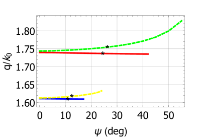
(a)

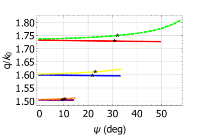
(b)

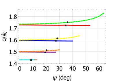
(c)

Figure 2: Plots of $q/k_{\scriptscriptstyle 0}$ versus $\psi$ for $\chi=0^{\circ}$ and $\gamma=1$, when (a) $\varepsilon^{s}_{\cal A}=2.5$, (b) $\varepsilon^{s}_{\cal A}=2.2,$ and (c) $\varepsilon^{s}_{\cal A}=2$. The curves represent DT surface-wave solutions: there are 4 branches for (a), 6 for (b), and 8 for (c). On each branch, the corresponding DTV surface-wave solution is identified by a star.

In Figs. 2(a-c) plots are provided of $q/k_{\scriptscriptstyle 0}$ versus $\psi$, as obtained from Eq. (38). For these calculations $\chi=0^{\circ}$ and $\gamma=1$, with (a) $\varepsilon^{s}_{\cal A}=2.5$, (b) $\varepsilon^{s}_{\cal A}=2.2,$ and (c) $\varepsilon^{s}_{\cal A}=2$. Representing DT surface waves, the solutions organized as branches: there are 4 branches for $\varepsilon^{s}_{\cal A}=2.5$, 6 for $\varepsilon^{s}_{\cal A}=2.2$, and 8 for $\varepsilon^{s}_{\cal A}=2$. Each branch exists for a continuous range of $q$, say $q_{\text{min}}<q<q_{\text{max}}$ and a continuous range of $\psi$, say $\psi_{\text{min}}<\psi<\psi_{\text{max}}$. For every branch, $\psi_{\text{min}}=0^{\circ}$, while $\psi_{\text{max}}\in\left(11^{\circ},64^{\circ}\right)$ depending on the value of $\varepsilon^{s}_{\cal A}$. The solution branches that arise at higher values of $q_{\text{min}}$ exist for wider ranges of values of $\psi$. The value of $q$ on each branch increases slowly as $\psi$ increases towards $\psi_{\text{max}}$.

On every DT branch in Figs. 2(a-c), for a unique value of $\psi$ and a unique value of $q$, there exists a DTV surface-wave solution — which is represented by a star. These DTV solutions do not arise at $\psi\in\left\{\psi_{\text{min}},\psi_{\text{max}}\right\}$ nor at $q\in\left\{q_{\text{min}},q_{\text{max}}\right\}$; instead, they arise at mid-range values of $\psi$ and $q$.

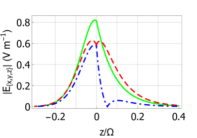
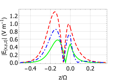
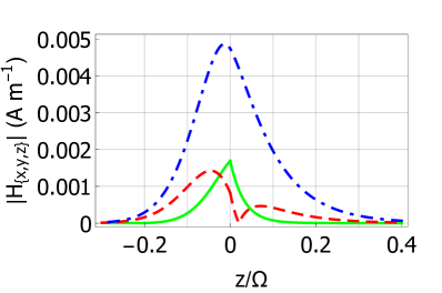
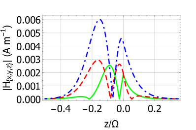
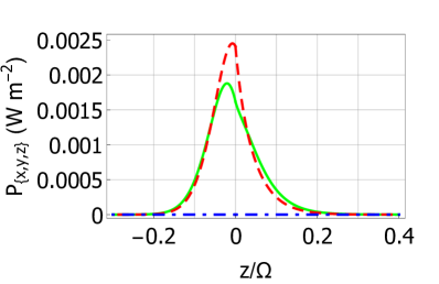
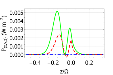
Figure 3: Field profiles for (left) a DT surface wave and (right) a DTV surface wave. Components of the quantities $|\underline{E}(z\hat{\underline{u}}_{\,z})\mbox{ \tiny{${}^{\bullet}$} }\underline{n}|$, $|\underline{H}(z\hat{\underline{u}}_{\,z})\mbox{ \tiny{${}^{\bullet}$} }\underline{n}|$, and $\underline{P}(z\hat{\underline{u}}_{\,z})\mbox{ \tiny{${}^{\bullet}$} }\underline{n}$ are plotted versus $z/\Omega$, for $\varepsilon^{s}_{\cal A}=2.2$, $\varepsilon^{t}_{\cal A}=4$, and $\chi=0^{\circ}$ with $C_{\mathcal{B}3}=1$ V m^-1. Left: $\psi=53^{\circ}$, $q=1.786\,k_{\scriptscriptstyle 0}$; Right: $\psi=22.993^{\circ}$ , $q=1.6198\,k_{\scriptscriptstyle 0}$. Key: $\underline{n}=\hat{\underline{u}}_{x}$ green solid curves; $\underline{n}=\hat{\underline{u}}_{y}$ red dashed curves; $\underline{n}=\hat{\underline{u}}_{z}$ blue broken-dashed curves.

The nature of the surface-wave solutions presented in Fig. 2 is further illuminated in Fig. 3 wherein spatial profiles of the magnitudes of the Cartesian components of the electric and magnetic field phasors are provided for a DT surface wave and a DTV surface wave. As representative examples, $\psi=53^{\circ}$ and $q=1.786\,k_{\scriptscriptstyle 0}$ were selected for the DT surface wave, whereas $\psi=22.993^{\circ}$ and $q=1.6198\,k_{\scriptscriptstyle 0}$ were selected for the DTV surface wave. In both cases, for $z\lessapprox-0.2\,\Omega$ and $z\gtrapprox 0.05\,\Omega$, the magnitudes of the components of the electric and magnetic field phasors displayed in Fig. 3 decay exponentially as the distance $|{z}|$ from the interface plane increases. The rates of decay in material ${\cal A}$ and material ${\cal B}$ are similar. Hence, it may be inferred that the linear decay in Eq. (20) is dominated by the exponential decay for $z\gtrapprox 0.05\,\Omega$.

Insight in to the localization of the surface waves is also provided by profiles of the Cartesian components of the time-averaged Poynting vector

$$\underline{P}(\underline{r})=\frac{1}{2}\mbox{Re}\left\{\,\underline{E}(\underline{r})\times\underline{H}^{*}(\underline{r})\,\right\}$$ (39)

that are presented in Fig. 3. These profiles show that energy flow for both the DT and the DTV surface waves is concentrated in directions parallel to the interface plane $z=0$. Furthermore, the energy densities of the surface waves are concentrated not at the interface $z=0$, but at a distance of approximately $0.15\,\Omega$ from the interface in material ${\cal B}$ for the DTV wave, and a distance of approximately $0.02\,\Omega$ from the interface in material ${\cal B}$ for the DT wave.

Let us consider further the anatomy of the DTV surface-wave solution, as provided in Eq. (20) for $z>0$. Three contributions to $\left[\underline{f}(z)\right]$ may be identified, namely

$$\left[\underline{f}(z)\right]=\left[\underline{f}_{1}(z)\right]+\left[\underline{f}_{2}(z)\right]+\left[\underline{f}_{3}(z)\right],\qquad z>0,$$ (40)

wherein

$$\left.\begin{array}[]{l}\left[\underline{f}_{1}(z)\right]=C_{{\cal A}1}\left[\underline{v}_{{\cal A}}\right]\,\exp\left(i\alpha_{{\cal A}}z\right)\vspace{6pt}\\ \left[\underline{f}_{2}(z)\right]=C_{{\cal A}2}\left[\underline{w}_{{\cal A}}\right]\,\exp\left(i\alpha_{{\cal A}}z\right)\vspace{6pt}\\ \left[\underline{f}_{3}(z)\right]=C_{{\cal A}2}\left\{iz\left[\underline{v}_{{\cal A}}\right]\right\}\,\exp\left(i\alpha_{{\cal A}}z\right)\end{array}\right\}.$$ (41)

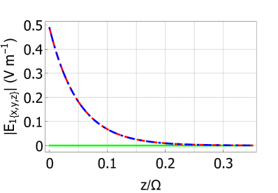
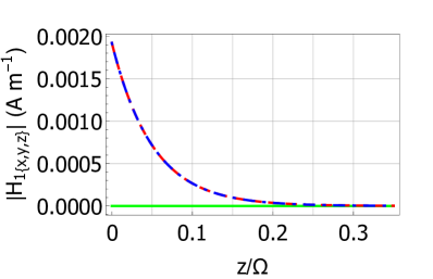
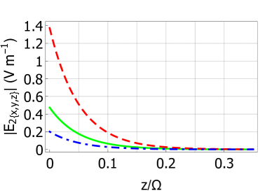
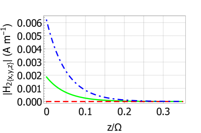
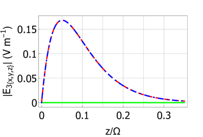
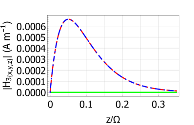
Figure 4: Field profiles for the contributions to the DTV surface-wave solution represented in Fig. 3 (right), per Eq. (40). Components of the quantities $|\underline{E}_{\ell}(z\hat{\underline{u}}_{\,z})\mbox{ \tiny{${}^{\bullet}$} }\underline{n}|$ and $|\underline{H}_{\ell}(z\hat{\underline{u}}_{\,z})\mbox{ \tiny{${}^{\bullet}$} }\underline{n}|$, where $\ell\in\left\{1,2,3\right\}$, are plotted versus $z/\Omega$, for $\varepsilon^{s}_{\cal A}=2.2$, $\varepsilon^{t}_{\cal A}=4$, and $\chi=0^{\circ}$ with $C_{\mathcal{B}3}=1$ V m^-1, with $\psi=22.993^{\circ}$ and $q=1.6198\,k_{\scriptscriptstyle 0}$. Key: $\underline{n}=\hat{\underline{u}}_{x}$ green solid curves; $\underline{n}=\hat{\underline{u}}_{y}$ red dashed curves; $\underline{n}=\hat{\underline{u}}_{z}$ blue broken-dashed curves.

The $x$ and $y$ components of the electric and magnetic field phasors are assembled to form the 4-vectors $\left[\underline{f}_{\ell}(z)\right]$ for $\ell=1,2,$ and 3, per Eq. (6). The corresponding $z$ components are delivered by means of Eqs. (9). Profiles of the magnitudes of the Cartesian components of the electric and magnetic field phasors comprising $\left[\underline{f}_{\ell}(z)\right]$, $\ell\in\left\{1,2,3\right\}$, are plotted for $z>0$ in Fig. 4, for the DTV surface-wave solution represented in Fig. 3. Close to the planar interface, i.e., for $z<0.05\Omega$, the magnitudes presented in Fig. 4 corresponding to the exponentially decaying contributions $\left[\underline{f}_{1}(z)\right]$ and $\left[\underline{f}_{2}(z)\right]$ are much larger than the magnitudes corresponding to the mixed linear-exponential contribution $\left[\underline{f}_{3}(z)\right]$. By comparing with the profiles of $|\underline{E}(z\hat{\underline{u}}_{\,z})\mbox{ \tiny{${}^{\bullet}$} }\underline{n}|$ and $|\underline{H}(z\hat{\underline{u}}_{\,z})\mbox{ \tiny{${}^{\bullet}$} }\underline{n}|$ with $\underline{n}\in\left\{\hat{\underline{u}}_{x},\hat{\underline{u}}_{y},\hat{\underline{u}}_{z}\right\}$ in Fig. 3 for $z>0$, we infer that the mixed linear-exponential contribution $\left[\underline{f}_{3}(z)\right]$ has a stronger effect on $|\underline{E}(z\hat{\underline{u}}_{\,z})\mbox{ \tiny{${}^{\bullet}$} }\hat{\underline{u}}_{z}|$ than on $|\underline{E}(z\hat{\underline{u}}_{\,z})\mbox{ \tiny{${}^{\bullet}$} }\hat{\underline{u}}_{x}|$ and $|\underline{E}(z\hat{\underline{u}}_{\,z})\mbox{ \tiny{${}^{\bullet}$} }\hat{\underline{u}}_{y}|$, and a stronger effect on $|\underline{H}(z\hat{\underline{u}}_{\,z})\mbox{ \tiny{${}^{\bullet}$} }\hat{\underline{u}}_{y}|$ than on $|\underline{H}(z\hat{\underline{u}}_{\,z})\mbox{ \tiny{${}^{\bullet}$} }\hat{\underline{u}}_{x}|$ and $|\underline{H}(z\hat{\underline{u}}_{\,z})\mbox{ \tiny{${}^{\bullet}$} }\hat{\underline{u}}_{z}|$.

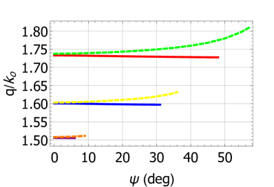
(a)

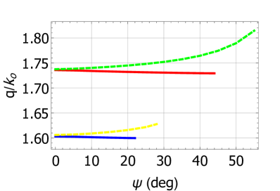
(b)

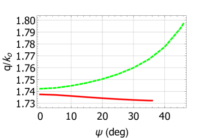
(c)

Figure 5: Plots of $q/k_{\scriptscriptstyle 0}$ versus $\psi$ for $\gamma=1$ and $\varepsilon^{s}_{\cal A}=2.2$, when (a) $\chi=10^{\circ}$, (b) $\chi=20^{\circ}$, and (c) $\chi=30^{\circ}$. The curves represent DT surface-wave solutions: there are 6 branches for (a), 4 for (b), and 2 for (c).

The influence of the orientation of the optic axis of material ${\cal A}$ is taken up in Figs. 5(a-c), wherein plots of $q/k_{\scriptscriptstyle 0}$ versus $\psi$ are provided for (a) $\chi=10^{\circ}$, (b) $\chi=20^{\circ}$, and (c) $\chi=30^{\circ}$. For these calculations, $\gamma=1$ and $\varepsilon^{s}_{\cal A}=2.2$. The DT surface-wave solutions are organized as 6 branches for $\chi=10^{\circ}$, 4 branches for $\chi=20^{\circ}$, and 2 branches for $\chi=30^{\circ}$. The characteristics of the $q/k_{\scriptscriptstyle 0}$ vs. $\psi$ curves in Figs. 5 and 2 are quite similar. The number of DT branches decreases as $\chi$ increases, with no DT surface-wave solutions at all being found for $\chi>45^{\circ}$.

Not a single DTV surface-wave solution exists in Fig. 5. Indeed, no DTV surface-wave solution was found by us for $\chi>0^{\circ}$. An analogous result holds for Dyakonov–Voigt surface waves [35].

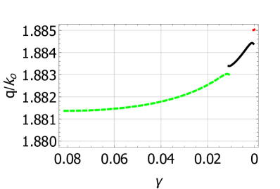
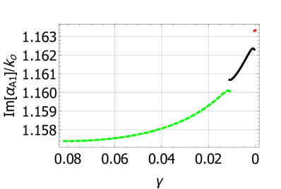
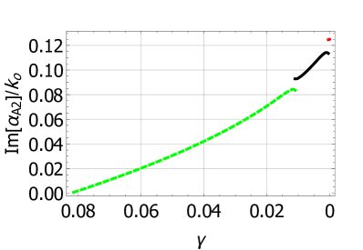
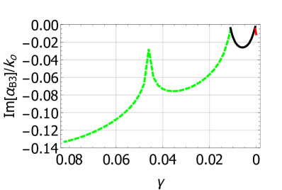
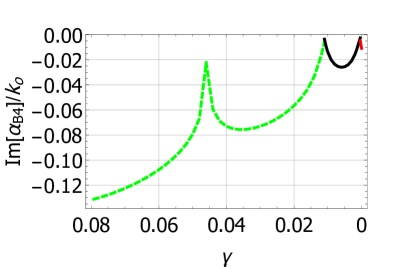
Figure 7: Plots of $q/k_{\scriptscriptstyle 0}$, $\mbox{Im}\left\{\alpha_{{\cal A}1}\right\}/k_{\scriptscriptstyle 0}$, $\mbox{Im}\left\{\alpha_{{\cal A}2}\right\}/k_{\scriptscriptstyle 0}$, $\mbox{Im}\left\{\alpha_{{\cal B}3}\right\}/k_{\scriptscriptstyle 0}$, and $\mbox{Im}\left\{\alpha_{{\cal B}4}\right\}/k_{\scriptscriptstyle 0}$ versus $\gamma$, for $\psi=66.5^{\circ}$, $\varepsilon^{s}_{\cal A}=2.2$, and $\chi=0^{\circ}$. The curves represent DT surface-wave solutions: there is only one branch for $\gamma<0.082$.

The influence of the amplitude of periodic variation in dielectric properties along the negative $z$ axis is taken up in Figs. 6 and 7. Plots of $q/k_{\scriptscriptstyle 0}$, $\mbox{Im}\left\{\alpha_{{\cal A}1}\right\}/k_{\scriptscriptstyle 0}$, $\mbox{Im}\left\{\alpha_{{\cal A}2}\right\}/k_{\scriptscriptstyle 0}$, $\mbox{Im}\left\{\alpha_{{\cal B}3}\right\}/k_{\scriptscriptstyle 0}$, and $\mbox{Im}\left\{\alpha_{{\cal B}4}\right\}/k_{\scriptscriptstyle 0}$, versus $\gamma$ are presented in Fig. 6 for $\psi=30^{\circ}$, $\chi=0^{\circ}$, and $\varepsilon^{s}_{\cal A}=2.2$. There are 4 branches of DT surface-wave solutions for $0.12<\gamma\leq 1$ and 2 branches for $0<\gamma<0.12$. The quantities $q/k_{\scriptscriptstyle 0}$, $\mbox{Im}\left\{\alpha_{{\cal A}1}\right\}/k_{\scriptscriptstyle 0}$, and $\mbox{Im}\left\{\alpha_{{\cal A}2}\right\}/k_{\scriptscriptstyle 0}$ all increase uniformly as $\gamma$ decreases, whereas $\mbox{Im}\left\{\alpha_{{\cal B}3}\right\}/k_{\scriptscriptstyle 0}$ and $\mbox{Im}\left\{\alpha_{{\cal B}4}\right\}/k_{\scriptscriptstyle 0}$ generally increase as $\gamma$ decreases. For the 2 branches that exist for $0<\gamma<0.12$, both $\mbox{Im}\left\{\alpha_{{\cal B}3}\right\}/k_{\scriptscriptstyle 0}$ and $\mbox{Im}\left\{\alpha_{{\cal B}4}\right\}/k_{\scriptscriptstyle 0}$ become null valued in the limit as $\gamma$ approaches zero. Accordingly, these 2 branches do not represent surface waves in the limiting case $\gamma\to 0$ because the conditions $\mbox{Im}\left\{\alpha_{{\cal B}3}\right\}/k_{\scriptscriptstyle 0}<0$ and $\mbox{Im}\left\{\alpha_{{\cal B}4}\right\}/k_{\scriptscriptstyle 0}<0$, which must be satisfied for surface-wave propagation, are not then satisfied.

In Fig. 7 plots analogous to those for Fig. 6 are provided for the case of $\psi=66.5^{\circ}$. In order to better illustrate the regime in which $\gamma$ approaches zero, the plots in Fig. 7 focus on the range $\gamma\in\left[0.082,0\right)$. In this case there is only one branch of DT surface-wave solutions. No DTV surface-wave solutions exist in $\gamma\in\left[1,0.082\right)$. All the quantities plotted in Fig. 7 generally increase as $\gamma$ decreases, albeit the curves for $q/k_{\scriptscriptstyle 0}$, $\mbox{Im}\left\{\alpha_{{\cal A}1}\right\}/k_{\scriptscriptstyle 0}$, and $\mbox{Im}\left\{\alpha_{{\cal A}2}\right\}/k_{\scriptscriptstyle 0}$ are discontinuous. The curves for $\mbox{Im}\left\{\alpha_{{\cal A}1}\right\}/k_{\scriptscriptstyle 0}$ and $\mbox{Im}\left\{\alpha_{{\cal A}2}\right\}/k_{\scriptscriptstyle 0}$ are similar, and so are the curves for $\mbox{Im}\left\{\alpha_{{\cal B}3}\right\}/k_{\scriptscriptstyle 0}$ and $\mbox{Im}\left\{\alpha_{{\cal B}4}\right\}/k_{\scriptscriptstyle 0}$. Unlike in Fig. 6, $\mbox{Im}\left\{\alpha_{{\cal B}3}\right\}/k_{\scriptscriptstyle 0}$ and $\mbox{Im}\left\{\alpha_{{\cal B}4}\right\}/k_{\scriptscriptstyle 0}$ do not become null valued as $\gamma$ approaches zero in Fig. 7; instead, both $\mbox{Im}\left\{\alpha_{{\cal B}3}\right\}/k_{\scriptscriptstyle 0}$ and $\mbox{Im}\left\{\alpha_{{\cal B}4}\right\}/k_{\scriptscriptstyle 0}$ are approximately equal to $-0.01$ as $\gamma$ approaches zero. In the limiting case $\gamma\to 0$, material ${\cal B}$ becomes a homogeneous material and the corresponding surface-wave solution represents a Dyakonov surface wave [2, 4]. Indeed, analytic formulas yield the angular existence domain $66.42^{\circ}<\psi<67.45^{\circ}$, and the corresponding $q/k_{\scriptscriptstyle 0}$ range $1.8850<q/k_{\scriptscriptstyle 0}<1.8895$, for the corresponding Dyakonov wave that exists at $\gamma=0$; the values of $\psi$ and $q/k_{\scriptscriptstyle 0}$ for the surface-wave solution represented in Fig. 7 lie within these ranges as $\gamma$ approaches zero.

4 Closing remarks

The theory underpinning the propagation of Dyakonov–Tamm (DT) surface waves and Dyakonov–Tamm–Voigt (DTV) surface waves was formulated for the canonical boundary-value problem involving the planar interface of a homogeneous uniaxial dielectric material and a periodically nonhomogeneous isotropic dielectric material. Numerical studies were carried out with values corresponding to a realistic rugate filter [30, 31] for the highest and lowest refractive indexes of the periodically nonhomogeneous partnering material. Multiple DT surface waves were found to exist at a fixed propagation direction in the interface plane, depending upon the constitutive parameters of the partnering materials. These multiple solutions can be organized as continuous branches when regarded as functions of the propagation angle in the interface plane. Provided that the optic axis of the uniaxial partnering material lies in the interface plane, a single DTV surface-wave solution exists at a unique propagation direction on each solution branch.

The existence of multiple DT branch solutions — which is consistent with theoretical [8, 9, 13, 14, 15], and experimental [16, 17] studies of DT surface waves supported by the planar interface of a homogeneous isotropic material and a periodically-nonhomogeneous anisotropic material — is a feature that could be usefully exploited in optical sensing applications [12], for example.

The unusual localization characteristics of DTV surface waves mirror those of Dyakonov–Voigt surface waves [40, 35] and surface-plasmon-polariton–Voigt waves [41]. While the existence of DTV surface waves is established theoretically herein for an idealized scenario, i.e., the canonical boundary-value problem, further studies are required to elucidate the excitation of such waves and their propagation for partnering materials of finite thicknesses.

Acknowledgments. This work was supported by EPSRC (grant number EP/S00033X/1) and US NSF (grant number DMS-1619901). AL thanks the Charles Godfrey Binder Endowment at the Pennsylvania State University and the Otto Mønsted Foundation for partial support of his research endeavors.

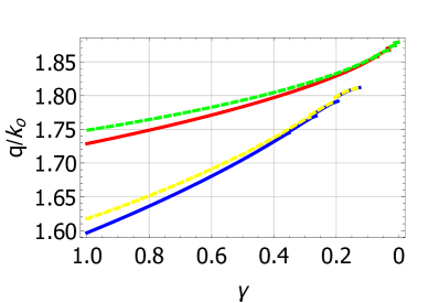
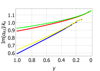
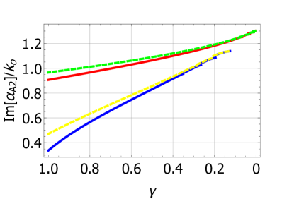
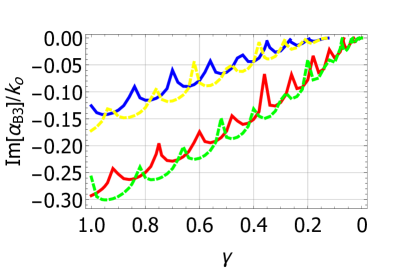
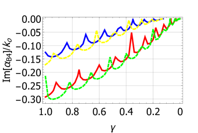
Figure 6: Plots of $q/k_{\scriptscriptstyle 0}$, $\mbox{Im}\left\{\alpha_{{\cal A}1}\right\}/k_{\scriptscriptstyle 0}$, $\mbox{Im}\left\{\alpha_{{\cal A}2}\right\}/k_{\scriptscriptstyle 0}$, $\mbox{Im}\left\{\alpha_{{\cal B}3}\right\}/k_{\scriptscriptstyle 0}$, and $\mbox{Im}\left\{\alpha_{{\cal B}4}\right\}/k_{\scriptscriptstyle 0}$ versus $\gamma$, for $\psi=30^{\circ}$, $\varepsilon^{s}_{\cal A}=2.2$, and $\chi=0^{\circ}$. The curves represent DT surface-wave solutions: there are 4 branches for $0.12<\gamma\leq 1$ and 2 branches for $0<\gamma<0.12$.

References

- [1] A.D. Boardman (editor), Electromagnetic Surface Modes, Wiley, Chicester, UK, 1982.
- [2] J.A. Polo Jr., T.G. Mackay, A. Lakhtakia, Electromagnetic Surface Waves: A Modern Perspective, Elsevier, Waltham, MA, USA, 2013.
- [3] F.N. Marchevskiĭ, V.L. Strizhevskiĭ, S.V. Strizhevskiĭ, Singular electromagnetic waves in bounded anisotropic media, Sov. Phys. Solid State 26 (1984) 911–912.
- [4] M.I. D’yakonov, New type of electromagnetic wave propagating at an interface, Sov. Phys. JETP 67 (1988) 714–716.
- [5] O. Takayama, L. Crasovan, D. Artigas, L. Torner, Observation of Dyakonov surface waves, Phys. Rev. Lett. 102 (2009) 043903.
- [6] O. Takayama, L.C. Crasovan, S.K. Johansen, D. Mihalache, D. Artigas, L. Torner, Dyakonov surface waves: A review, Electromagnetics 28 (2008) 126–145.
- [7] D.B. Walker, E.N. Glytsis, T.K. Gaylord, Surface mode at isotropic-uniaxial and isotropic-biaxial interfaces, J. Opt. Soc. Am. A 15 (1998) 248–260.
- [8] A. Lakhtakia, J.A. Polo Jr., Dyakonov–Tamm wave at the planar interface of a chiral sculptured thin film and an isotropic dielectric material, J. Eur. Opt. Soc. Rapid Publ. 2 (2007) 07021.
- [9] J.A. Polo Jr., A. Lakhtakia, Dyakonov–Tamm waves guided by the planar interface of an isotropic dielectric material and an electro-optic ambichiral Reusch pile, J. Opt. Soc. Am. B 28 (2011) 567–576.
- [10] O. Takayama, D. Artigas. L. Torner, Practical dyakonons, Opt. Lett. 37 (2012) 4311–4313.
- [11] O. Takayama, D. Artigas. L. Torner, Coupling plasmons and dyakonons, Opt. Lett. 37 (2012) 1983–1985.
- [12] A. Lakhtakia. M. Faryad, Theory of optical sensing with Dyakonov–Tamm waves, J. Nanophoton. 8 (2014) 083072.
- [13] A. Lakhtakia, M. Faryad, Dyakonov–Tamm waves guided jointly by an ordinary, isotropic, homogeneous, dielectric material and a hyperbolic, dielectric, structurally chiral material, J. Modern Opt. 61 (2014) 1115–1119.
- [14] F. Chiadini, V. Fiumara, T.G. Mackay, A. Scaglione, A Lakhtakia, Temperature-mediated transition from Dyakonov–Tamm surface waves to surface-plasmon-polariton waves, J. Opt. (UK) 19 (2017) 085002.
- [15] T.G. Mackay, A. Lakhtakia, High-phase-speed Dyakonov–Tamm surface waves, J. Nanophoton. 11 (2017) 030501.
- [16] D.P. Pulsifer, M. Faryad, A. Lakhtakia, Observation of the Dyakonov–Tamm wave, Phys. Rev. Lett. 111 (2013) 243902.
- [17] D.P. Pulsifer, M. Faryad, A. Lakhtakia, A.S. Hall, L. Liu, Experimental excitation of the Dyakonov–Tamm wave in the grating-coupled configuration, Opt. Lett. 39 (2013) 2125–2128.
- [18] W. Voigt, On the behaviour of pleochroitic crystals along directions in the neighbourhood of an optic axis, Phil. Mag. 4 (1902) 90–97.
- [19] G.N. Borzdov, Waves with linear, quadratic and cubic coordinate dependence of amplitude in crystals, Pramana–J. Phys. 46 (1996) 245–257.
- [20] M. Grundmann, C. Sturm, C. Kranert, S. Richter, R. Schmidt-Grund, C. Deparis, J. Zúiga-Pérez, Optically anisotropic media: New approaches to the dielectric function, singular axes, microcavity modes and Raman scattering intensities, Physica Status Solidi RRL 11 (2017) 1600295.
- [21] S. Pancharatnam, The propagation of light in absorbing biaxial crystals — I. Theoretical, Proc. Ind. Acad. Sci. A 42 (1955) 86–109.
- [22] B.N. Grechushnikov, A.F. Konstantinova, Crystal optics of absorbing and gyrotropic media, Comput. Math. Applic. 16 (1988) 637–655.
- [23] G.S. Ranganath, Optics of absorbing anisotropic media, Curr. Sci. (India) 67 (1994) 231–237.
- [24] J. Gerardin, A. Lakhtakia, Conditions for Voigt wave propagation in linear, homogeneous, dielectric mediums, Optik 112 (2001) 493–495.
- [25] H.C. Chen, Theory of Electromagnetic Waves, McGraw–Hill, New York, NY, USA, 1983.
- [26] T.G. Mackay, A. Lakhtakia, Electromagnetic Anisotropy and Bianisotropy: A Field Guide, 2nd Edition, World Scientific, Singapore, 2019.
- [27] T.H. O’Dell, The Electrodynamics of Magneto-electric Media, North-Holland, Amsterdam, The Netherlands, 1970.
- [28] J.F. Nye, Physical Properties of Crystals, Clarendon Press, Oxford, UK, 1985.
- [29] M. Born. E. Wolf, Principles of Optics, 6th Edition, Pergamon Press, Oxford, UK, 1980.
- [30] B.V. Bovard, Rugate filter theory: an overview, Appl. Opt. 32 (1993) 5427–5442.
- [31] P.W. Baumeister, Optical Coating Technology, SPIE Press, Bellingham, WA, USA, 2004.
- [32] J. Billard, Contribution a l’Etude de la Propagation des Ondes Electromagnetiques Planes dans Certains Milieux Materiels (2ème these), PhD Dissertation (Université de Paris 6, France), pp. 175–178, 1966.
- [33] D.W. Berreman, Optics in stratified and anisotropic media: 44-matrix formulation, J. Opt. Soc. Am. 62 (1972) 502–510.
- [34] M. Faryad, A. Lakhtakia, On surface-plasmon-polariton waves guided by the interface of a metal and a rugate filter with a sinusoidal refractive-index profile, J. Opt. Soc. Am. B 27 (2010) 2218–2223.
- [35] C. Zhou, T.G. Mackay, A. Lakhtakia, On Dyakonov–Voigt surface waves guided by the planar interface of dissipative materials, J. Opt. Soc. Am. B 36 (2019) 3218–3225.
- [36] W.E. Boyce, R.C. DiPrima, Elementary Differential Equations and Boundary Value Problems, 9th Edition, Wiley, Hoboken, NJ, USA, 2010.
- [37] H. Hochstadt, Differential Equations—A Modern Approach, Dover Press, New York, NY, USA, 1975.
- [38] V.A. Yakubovich, V.M. Starzhinskii, Linear Differential Equations with Periodic Coefficients, Wiley, Hoboken, NJ, USA, 1975.
- [39] Y. Jaluria, Computer Methods for Engineering, Taylor & Francis, Washington DC, USA, 1996.
- [40] T.G. Mackay, C. Zhou, A. Lakhtakia, Dyakonov–Voigt surface waves, Proc. R. Soc. A 475 (2019) 20190317.
- [41] C. Zhou, T.G. Mackay, A. Lakhtakia, Surface-plasmon-polariton wave propagation supported by anisotropic materials: multiple modes and mixed exponential and linear localization characteristics, Phys. Rev. A 100 (2019) 033809.