Towards Sharper First-Order Adversary with Quantized Gradients

Abstract

Despite the huge success of Deep Neural Networks (DNNs) in a wide spectrum of machine learning and data mining tasks, recent research shows that this powerful tool is susceptible to maliciously crafted adversarial examples. Up until now, adversarial training has been the most successful defense against adversarial attacks. To increase adversarial robustness, a DNN can be trained with a combination of benign and adversarial examples generated by first-order methods. However, in state-of-the-art first-order attacks, adversarial examples with sign gradients retain the sign information of each gradient component but discard the relative magnitude between components. In this work, we replace sign gradients with quantized gradients. Gradient quantization not only preserves the sign information, but also keeps the relative magnitude between components. Experiments show white-box first-order attacks with quantized gradients outperform their variants with sign gradients on multiple datasets. Notably, our BLOB_QG attack achieves an accuracy of $88.32\%$ on the secret MNIST model from the MNIST Challenge and it outperforms all other methods on the leaderboard of white-box attacks.

1 Introduction

Although Deep Neural Networks (DNN) are powerful tools in a wide range of applications, they are vulnerable to adversarial examples, which are crafted by adding small perturbations to benign examples [20]. Perturbations are so small that they are undetected by a human observer while they confuse well-trained DNNs to make wrong predictions, see Figure 1. Consequently, the lack of robustness of DNNs has raised significant concerns for safety in critical technologies such as autonomous driving and malware prevention [18, 6].

Figure 1: Perturbed MNIST by PQGD

One approach to increase adversarial robustness of DNNs is to train the model with data augumented by adversarial examples. In particular, [13] suggests the following Empirical Risk Minimization (ERM) as the objective:

$$\min_{\theta} \rho(\theta)$$ (1)

$$\textrm{where}\quad\rho(\theta) =\mathbb{E}_{(x,y)\sim\mathcal{D}}\big{[}\max_{\delta\in\mathcal{S}}L(\theta,x+\delta,y)\big{]}$$

Where $\theta$ denotes the parameters of DNNs, data examples $x$ with labels $y$ are from the data distribution $\mathcal{D}$ and $L(\theta,x,y)$ is the loss function of DNN. $\mathcal{S}$ is a set of allowed perturbations for crafting adversarial examples. In this paper, we consider the well studied $\ell_{\infty}$ perturbations, i.e., given some small threshold $\epsilon$, we have $\|\delta\|_{\infty}\leq\epsilon$ and it implies small visible changes in images for each pixel. Most of the first-order attacks used for adversarial training are crafted under $\ell_{\infty}$ perturbations. Solving the inner maximization problem equals to finding adversarial examples that the neural network fails to classify correctly while the outer minimization problem tends to increase the robustness against such adversaries.

Raw Gradients To solve the inner maximization problem of ERM in Eq. 1, one class of approach uses first-order methods to compute the perturbation $\delta$ and generate the adversarial example $x+\delta$. However, raw gradients $\nabla_{x}L(\theta,x,y)$ cannot be directly applied to images $x$, because magnitudes of raw gradients are at a different scale to the image pixels. For example, for the MNIST dataset, most components of raw gradients concentrate at values ranging from $10^{-5}$ to $10^{-4}$, while the pixel value of MNIST images belongs to the set $\{0,1/256,\ldots,1\}$.

Sign Gradients  To make use of raw gradients and apply them to pixel values, reseachers consider taking the sign of each raw gradient. In particular, the Fast Gradient Sign Method (FGSM) [7] linearizes the inner maximization problem with

$$x_{FGSM}=x+\epsilon\cdot\textrm{sgn}(\nabla L(\theta,x,y))$$ (2)

Note that $\textrm{sgn}(\nabla L(\theta,x,y))$ takes the sign of gradients $\nabla L(\theta,x,y)$, i.e., gradient values belong to the set of $\{-1,1\}$. A more sophisticated approach to generate adversarial examples is to use multi-step FGSM with a smaller step size $\alpha$, e.g., Iterative FGSM [11] and Projected Gradient Descent (PGD) attack [13]. Evidence in [13] has shown that the PGD attack is the universal first-order adversary.

Quantized Gradient  One limitation of sign gradients is that it discards the relative magnitude between each component of the raw gradient. When a component of raw gradient has its absolute value much larger than another component, it plays a more important role in solving the inner maximization problem. However, sign gradients only make the two components share the same absolute value of 1. Because a smaller step size $\alpha$ is used to generate adversarial examples, we consider taking gradient values from a wider range of integers than $\{-1,1\}$. Inspired by the success of quantized gradients [1] in distributed optimization, we introduce Quantized Gradients in first-order attacks to preserve the relative magnitude. Not only do quantized gradients retain the sign of each component, they also round each component to an integer proportional to its magnitude to preserve the relative magnitude. See Table 1 for the comparison between raw gradients, sign gradients and quantized gradients.

Gradient Scheme	Applicable on Pixels	Sign Preservation	Relative Magnitude Preservation
Raw Gradients	✗	✓	✓
Sign Gradients	✓	✓	✗
Quantized Gradients	✓	✓	✓

Table 1: Comparison of different gradient schemes

Our contributions are summarized as follows:

• We introduce generalized quantized gradients which can replace the sign gradients in existing first order attacks. Specifically, in this paper, we propose Projected Quantized Gradients Descent (PQGD) and DAA-BLOB with quantized gradients (BLOB_QG) as extensions of state-of-the-art first-order attacks PGD and DAA-BLOB.

• We show that PQGD and BLOB_QG are sharper attacks than PGD and DAA-BLOB, respectively, on multiple datasets. In particular, BLOB_QG achieves an accuracy of 88.32% on the secret MNIST model of the MNIST challenge and it outperforms all other methods on the leaderboard of white-box attacks. See Section 4.2.

• We study the effect of maximum allowed perturbation and number of steps on PQGD. Particularly, when maximum allowed perturbation is larger or step number is smaller, adversarial examples generated by PQGD are sharper than PGD. See details in Section 4.3 and 4.4.

• Our technique is simple to implement as it only requires tuning a single hyperparameter $b$.

2 Preliminaries

Given an $L-$class neural network classifier $f\mathrel{\mathop{\mathchar 58\relax}}\mathcal{R}^{d}\to\mathcal{R}^{L}$, for each $d-$dimensional data example $x$ and its corresponding ground truth label $y$, a $f$ is trained to match the predicted label $\hat{y}=\operatorname*{arg\,max}_{k}f_{k}(x)$ with the true label $y$ where $f_{k}(x)$ is the $k$th component of $f(x)$. To attack a well-trained classifier, an adversarial example $x_{adv}$ is crafted so that $\hat{y}_{adv}\neq\hat{y}$ where $\hat{y}_{adv}=\operatorname*{arg\,max}_{k}f_{k}(x_{adv})$ given perturbations $\|x_{adv}-x\|_{\infty}\leq\epsilon$.

Attacks can be divided into two main categories as summarized below:

• Targeted Attack and Untargeted Attack  By specifying a label $y^{\prime}\neq\hat{y}$, an adversarial example $x_{adv}$ is generated with its predicted label $\hat{y}_{adv}=y^{\prime}$ under the $\ell_{\infty}$ constraint. It is known as the targeted attack. On the other hand, an untargeted attack only requires $\hat{y}_{adv}$ to be any label except $\hat{y}$.

• White-box Attack and Black-box Attack  If the attack has access to all information of the network and training dataset, it is known as the white-box attack. FGSM and PGD attacks belong to this category because gradients are computed from network parameters and dataset. In contrast, the capability of attackers is more restricted in the black-box attack setting. In this scenario, attackers do not know the network parameters and network architecture, also access to any large training dataset is forbidden. See [14, 15] for a detailed description of black-box attacks.

In this paper, we consider white-box untargeted attacks under $\ell_{\infty}$ perturbations. We now present a state-of-the-art first-order attack known as Projected Gradient Descent attack.

Projected Gradient Descent (PGD) [13] is shown to be the universal first-order adversary. That is, a neural network trained with adversarial examples crafted using PGD is robust to any first-order attack. Given a chosen parameter $\alpha$, a training example $x$ and its label $y$, PGD is similar to the Iterative FGSM attack [11] and applies the following updates at iteration $t$ :

$$x^{(t+1)}=\Pi_{clip}(x^{(t)}+\alpha\cdot\textrm{sgn}(\nabla L(\theta,x^{(t)},y)))$$ (3)

Note that PGD is different from iterative FGSM in that $x_{0}$ is randomly perturbed in the vicinity of $x$, while iterative FGSM has $x_{0}=x$. On the other hand, FGSM uses $\epsilon$ as the step size while PGD uses $\alpha$ where $\alpha$ is much smaller than $\epsilon$ in practice. For example, to craft MNIST adversarial examples, one has $\epsilon=0.3$ and $\alpha=0.01$.

3 Proposed Method

In this section, we extend first-order attacks with quantized gradients.

3.1 Motivation

Because of the $\ell_{\infty}$ constraint on the perturbation, each component of the perturbation is valid to take any value from the interval of $[-\epsilon,\epsilon]$. Using the sign gradient allows the perturbation at each iteration to take values from the set $\{-\alpha,+\alpha\}$. One challenge in PGD attacks is to determine other valid perturbations in each iteration leads to better attack. We seek for a solution to the problem. Note that existing works attempt to craft first-order attacks with sign gradients, so the absolute value of the perturbation at each iteration is equal to the step size $\alpha$. Our research uses different perturbation values for each component to craft a shaper attack, for this reason our work is orthogonal to existing research on first-order attacks.

We first introduce the technique of gradient quantization and propose a generalized gradient quantization to show that existing sign gradient attack can be replaced with the quantized gradient. We inspect the distribution of perturbation values of quantized gradients, sign gradients and raw gradients. Finally, we analyze the time complexity of our approach compared with vanilla sign gradients.

3.2 Gradient Quantization

Our approach attempts to preserve the relative magnitude between each component in the raw gradient while it is still applicable on pixel value as shown in Table 1. Given a positive integer hyperparameter $b$, data example $x$ and its corresponding label $y$, the loss function $L$ and network parameters $\theta$, we calculate quantized gradient $\mathbf{qg}$ as follows:

1. Calculate the gradient of loss function $\mathbf{g}=\nabla_{x}L(\theta,x,y)$

2. Take the max value of components in the gradient $M=\max_{i}{\mathinner{\!\left\lvert g_{i}\right\rvert}}$

3. Return the quantized gradient $\mathbf{qg}=\zeta(b\cdot g/M)$

.

Where function $\zeta(\cdot)$ aims to round each component to its nearest integer except when the absolute value of the component is less than 1. Specifically, it takes the following form:

$$\zeta(v_{i})=\begin{cases}\textrm{sgn}(v_{i})&\text{if}\,\mathinner{\!\left\lvert v_{i}\right\rvert}<1,\\ \textrm{round}({v_{i}})&\text{otherwise.}\end{cases}$$ (4)

The $\zeta$ function enforces each component of $\mathbf{qg}$ to be non-zero integer. Function $\textrm{round}({v_{i}})$ rounds $v_{i}$ to its nearest integer.

Relationship to Sign Gradients In the special case where $b=1$, quantized gradient $\mathbf{qg}$ degenerates to sign gradient which is used in the current FGSM and PGD framework.

Note that only one hyperparameter $b$ needs to be tuned when computing the quantized gradient $\mathbf{qg}$. When $b$ is set to a large integer, the relative magnitude between each component of the raw gradient is preserved. Each component of the perturbation is rescaled to an integer belonging to $[-b,b]$.

Indeed, gradient quantization is equivalent to finding a scheme to assign different step size to each component of the perturbation. We later show this method of assignment helps to craft more effective adversarial examples, where fewer iterations are needed to generate sharper adversarial examples than sign gradients. For adversarial training, it is too expensive to augument adversarial examples which needs many iterations to generate. If adversarial examples of similar effectiveness can be generated using fewer iterations, adversarial training can benefit from such examples.

Connection to QSGD We briefly review how quantized gradients are used in distributed optimization. In distributed optimization, one of the bottlenecks in performance is the limited bandwidth required to collect gradients from several parallel machines. Quantized Stochastic Gradient Descent (QSGD)[1] is proposed to conserve the bandwidth with a good convergence gurantee. To be specific, each component of the gradient is quantized and randomly rounded to a discrete set of values. Given any gradient $\mathbf{v}\in\mathcal{R}^{d}$ and a hyperparameter $s$, the quantized gradient $Q_{s}(\mathbf{v})$ is defined as:

$$Q_{s}(v_{i})=\|\mathbf{v}\|_{2}\cdot sgn(v_{i})\cdot\xi_{i}(\mathbf{v},s)$$ (5)

Given some positive integer $l$ such that $\mathinner{\!\left\lvert v_{i}\right\rvert}/\|\mathbf{v}\|_{2}\in\big{[}l/s,(l+1)/s\big{]}$, $\xi_{i}(\mathbf{v},s)$ is given by

$$\xi_{i}(\mathbf{v},s)=\begin{cases}l/s&\text{with probability}\,p\\ (l+1)/s&\text{otherwise}\end{cases}$$ (6)

where $p=1-(\frac{\mathinner{\!\left\lvert v_{i}\right\rvert}}{\|\mathbf{v}\|_{2}}\cdot s-l)$. Experiments show that QSGD significantly outperforms its full-precision variant in terms of convergence speed.

Although quantized gradients used in attacks bear some resemblance to QSGD, there are a few differences between the two quantization techniques.

• QSGD is a randomized approach whereas our method is deterministic. In particular, QSGD randomly rounds every component to the nearest floor integer or ceiling integer, while our approach rounds every component using the deterministic function $\zeta(\cdot)$.

• QSGD uses $\ell 2$-norm of the gradient to divide each component. On the other hand, we enforce the $\ell_{\infty}$ constraint on the perturbation. So we use $\|\mathbf{g}\|_{\infty}=\max_{i}{\mathinner{\!\left\lvert g_{i}\right\rvert}}$ to divide each component.

• QSGD has its component $Q_{s}(v_{i})\in[0,1]$, while our approach constrains each component of $\mathbf{qg}$ as any non-zero integer.

3.3 Generalized Gradient Quantization

Here, we introduce generalized gradient quantization for first-order attacks.

Recall that at each iteration PGD update has the form of Eq. 3. To integrate quantized gradients with PGD, we replace the sign gradient $\text{sgn}(\nabla_{x}L(\theta,x,y))$ with $\mathbf{qg}$. It takes the following form:

$$x^{(t+1)}=\Pi_{clip}(x^{(t)}+\alpha\cdot\mathbf{qg})$$ (7)

We name our approach Projected Quantized Gradient Descent (PQGD). To facilitate other existing first-order attacks with sign gradients, i.e., for attacks with the form $x^{(t+1)}=\Pi_{clip}(x^{(t)}+\alpha\cdot sgn(\cdot))$, we replace $sgn(\cdot)$ with the quantized gradients to improve the effectiveness of attacks. We call this approach generalized gradient quantization.

Distributionally Adversarial Attack (DAA) is an example of a state-of-the-art first-order white-box attack, which appears on the leaderboard of the MNIST challenge. While DAA is proposed to solve the optimal adversarial data distribution [25], PGD views each data example independently. DAA is interpreted as Wasserstein Gradient Flows, and the update of DAA using the Lagranigian Blob Method (DAA-BLOB) at iteration $t$ is given as:

$$\mathbf{eg}=\nabla_{x^{(t)}_{i}} L(\theta,x^{(t)}_{i},y_{i})+$$ (8)

$$\frac{c}{M}\big{[}\sum_{j=1}^{M} K(x^{(t)}_{i},x^{(t)}_{j})\nabla_{x^{(t)}_{j}}L(\theta,x^{(t)}_{j},y_{j})+$$

$$\nabla_{x^{(t)}_{j}} K(x^{(t)}_{i},x^{(t)}_{j})\big{]}$$

$$x^{(t+1)}_{i}=\Pi_{clip}(x^{(t)}_{i}+\alpha\cdot\textrm{sgn}(\mathbf{eg})$$ (9)

where $K(\cdot,\cdot)$ is a kernel function. We define the following quantized gradient for DAA-BLOB.

$$\mathbf{eqg}=\zeta(b\cdot\mathbf{eg}/M_{eg})\quad\text{where}\quad M_{eg}=\max_{i}{\mathinner{\!\left\lvert eg_{i}\right\rvert}}.$$ (10)

DAA-BLOB with quantized gradient (BLOB_QG) has the following update in each iteration:

$$x^{(t+1)}=\Pi_{clip}(x^{(t)}+\alpha\cdot\mathbf{eqg})$$ (11)

We name this approach DAA-BLOB with quantized gradient (BLOB_QG).

3.4 Inspection of Quantized Gradient

(a) sign gradients

(b) quantized gradients (b=100)

(c) quantized gradients (b=200)

(d) quantized gradients (b=500)

(e) quantized gradients (b=1000)

(f) raw gradient

Figure 2: Histograms of sign gradients, raw gradient and quantized gradients of MNIST model with various values of $b$.

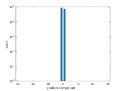
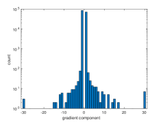
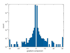
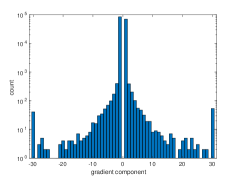
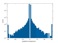
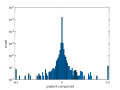
We plot the histogram of sign gradients, raw gradients and quantized gradients of the adversarial trained MNIST model with various values of $b$ (Fig. 2). Recall that an iterative attack has a projection operation at the end of each iteration. Therefore, the value change of each gradient component should be within the range of $[-\epsilon/\alpha,\epsilon/\alpha]$. Using MNIST as an example, we have a maximum allowed perturbation of $\epsilon=0.3$ and the learning rate of $\alpha=0.01$, so for the absolute value of gradient component larger than $\frac{\epsilon}{\alpha}=30$, the value will be clipped inside the range of $[-30,30]$.

Figure 2(a) shows the histogram of the sign gradient, which is used in PGD and other first-order attacks. Values of components of sign gradients concentrate on $\{-1,1\}$ because only the sign of each component is preserved. In Figure 2(b) to Figure 2(e), quantized gradients are spread out on the range of $[-30,30]$ and have a shape similar to the raw gradients shown in Figure 2(f). Not only is the sign of each component kept for quantized gradients, but the relative magnitude between each component is preserved.

Recall that we use function $\zeta(\cdot)$ to constrain each gradient component as non-zero integers. Thus, if we do not apply the constraint, most of the gradient components will have a value of $0$. Accordingly these components do not contribute to the crafting of adversarial examples. Therefore we enforce the components to be non-zero integers and they are restricted to the range $\{-1,1\}$, whose count dominates count of the other integer values within the range $[-30,30]$ as shown in Figure 2.

3.5 Complexity Analysis

We analyze the computational complexity of the quantized gradient here. Compared with vanilla gradients $\nabla_{x}L(\theta,x,y)$ has a time complexity of at least $\mathcal{O}(d)$ where $d$ is the dimension of data point $x$. Since computing the maximum $M$ and applying the function $\zeta$ takes time of $\mathcal{O}(d)$. Because of this, computing the quantized gradient shares the same time complexity as computing the raw gradient. Therefore, our technique introduces low computational overheads.

In addition, our approach of gradient quantization is easy to implement. For instance, in our python implementation, we use around 10 lines of code.

4 Experiment

The purpose of our experiment is to test the effectiveness of existing first-order attacks with quantized gradient (PQGD and BLOB_QG) on adversarial trained models compared to the attacks with sign gradients, e.g., PGD and DAA-BLOB.

4.1 Experiment Settings

Our code is based on the implementation of PGD and DAA-BLOB. The code of PGD can be found at code site and the implementation of DAA-BLOB can be found at code site. We use PGD, DAA-BLOB, Interval Attacks [22] and Surrogate attack [8] as the baselines in our experiment.

We compare our methods and baseline on the following datasets: MNIST [12], Cifar10[10], and Fashion-MNIST[23]. We mirror the architecture for MNIST and Cifar10 from the architecture used in [13] while we use the same architecture for Fashion-MNIST as that in [25]. We use default training configurations including batch size, learning rate and optimization settings. Cross entropy loss is used in all of our experiments.

Practical Issues  Since PGD and DAA-BLOB use randomly perturbed data examples to craft adversarial examples, adversarial examples generated in different runs are not exactly the same. An approach to take advantage of all different runs is to merge various adversarial examples that are misclassified by the classifier during different restarts.

4.2 Empirical Results

PGD		PQGD_100		PQGD_200		BLOB		BLOB_QG_100		BLOB_QG_200
Worst	Avg	Worst	Avg	Worst	Avg	Worst	Avg	Worst	Avg	Worst	Avg
92.56%	92.79%	92.27%	92.37%	92.17%	92.33%	90.48%	90.56%	90.07%	90.18%	90.08%	90.15%

Table 2: Performance Comparison of MIT MadryLab’s secret MNIST model without restart under 200-step attacks (0.3/1.0 $\ell_{\infty}$ perturbations). PQGD_100 denotes PQGD with $b=100$. BLOB is the DAA-BLOB approach. BLOB_QG_100 denotes DAA-BLOB with quantized gradients and $b=100$.

PGD	Interval Attack	BLOB	Surrogate	BLOB_QG_100	BLOB_QG_200	BLOB_QG_200 (100 runs)
89.49%	88.42%	88.56%	88.36%	88.40%	88.35%	88.32%

Table 3: Empirical worst-case accuracy of MIT MadryLab’s secret MNIST model under 200-step attacks (0.3/1.0 $\ell_{\infty}$ perturbations). In the last entry, we have BLOB_QG with 100 restarts. All other approaches are with 50 restarts. BLOB is the DAA-BLOB approach. BLOB_QG_100 denotes DAA-BLOB with quantized gradients and $b=100$.

MNIST We present the result of comparisons between our approach and baseline attacks on secret MNIST model in Tables 2 and 3. The secret MNIST model is taken from the Madry Lab’s MNIST-Challenge competition. We test attacks with quantized gradients with various values of $b$.

In Table 2, we compute the worst accuracy and average accuracy of five independent runs under a 200-step attack for each approach on the secret MNIST model. It shows results consistent with experiments from previous works [25] where DAA-BLOB outperforms PGD. Replacing sign gradients with quantized gradients boosts the performance of PGD and DAA-BLOB. Specifically, using quantized gradients in PGD decreases the worst accuracy of the secret MNIST model from 92.56% to 92.17% while using quantized gradients in DAA-BLOB decreases the worst accuracy from 90.48% to 90.07%.

We compare BLOB_QG with state-of-the-art methods appearing on the leaderboard of the MNIST challenge. Our BLOB_QG approach with $b=200$ and 100 restarts achieves a worst accuracy of $88.32\%$ and outperforms all other methods on the leaderboard of white-box attacks (In Table 3).

PGD		PQGD_100		PQGD_200		BLOB		BLOB_QG_100		BLOB_QG_200
Worst	Avg	Worst	Avg	Worst	Avg	Worst	Avg	Worst	Avg	Worst	Avg
71.11%	71.21%	70.79%	70.85%	70.66%	70.75%	67.90%	67.98%	67.33%	67.45%	67.30%	67.39%

Table 4: Performance Comparison of the adversarial trained Fashion-MNIST model without restart under 100-step attacks (0.2/1.0 $\ell_{\infty}$ perturbations). PQGD_100 denotes PQGD with $b=100$. BLOB is the DAA-BLOB approach. BLOB_QG_100 denotes DAA-BLOB with quantized gradients and $b=100$.

BLOB	BLOB_QG_100	BLOB_QG_200	BLOB_QG_500	BLOB_QG_1000
66.24%	65.78%	65.69%	65.61%	65.64%

Table 5: Empirical worst-case accuracy of the adversarial trained Fashion-MNIST model under 200-step attacks with 10 restarts (0.2/1.0 $\ell_{\infty}$ perturbations). BLOB is the DAA-BLOB approach. BLOB_QG_100 denotes DAA-BLOB with quantized gradients and $b=100$.

Fashion-MNIST We compare PQGD and BLOB-QG with baseline attacks on an adversarial trained Fashion-MNIST model in Tables 4 and 5. The adversarial Fashion-MNIST model is trained with adversarial examples generated by a 40-step PGD attack.

We observe results of Fashion-MNIST, which are consistent with those of MNIST. Existing attacks with quantized gradients create sharper attacks than those with sign gradients.

Perturbation	PGD	PQGD_100	PQGD_200	PQGD_500	PQGD_1000
8.0/255.0	45.31%	45.32%	45.32%	45.33%	45.57%
16.0/255.0	14.02%	14.24%	14.11%	13.98%	13.87%

Table 6: Performance Comparison of the adversarial trained Cifar10 model from Madry Lab with no restart under 100-step attack (with 8.0 and 16.0/255.0 $\ell_{\infty}maximumallowedperturbations$). PQGD_100 denotes PQGD with $b=100$.

Cifar10  We compare the performance of adversarial examples generated by PGD and PQGD on the adversarial trained Cifar10 model from the Madry Lab (in Table 6). We test a single run of 100-step attacks of PGD and PQGD under 8.0/255.0 and 16.0/255.0 $\ell_{\infty}$ maximum allowed perturbations.

As shown in Table 6, for a maximum allowed perturbation of 8.0/255.0. PQGD with $b=100,200,500$ achieves a similar performance to PGD. However, PQGD with $b=1000$ produces a worse result than PGD with an accuracy of $45.57\%$. On the other hand, for maximum allowed perturbations of 16.0/255.0, PQGD decreases the accuracy of adversarial trained models from $14.02\%$ to $13.87\%$. Interestingly, PQGD with $b=1000$ outperforms PGD under the $\ell_{\infty}$ maximum allowed perturbation of 16.0/255.0 whereas PGD outperforms PQGD under the maximum allowed perturbation of 8.0/255.0.

4.3 Effect Of Maximum Allowed Perturbation On Gradient Quantization

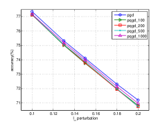
We plot the average accuracy of five independent runs of 100-step PQGD and PGD with different maximum allowed perturbations on the MNIST and Fashion-MNIST dataset (Fig. 3).

(a) MNIST

(b) Fashion-MNIST

Figure 3: Effect of Maximum Allowed Perturbation on the averaged accuracy of applying PQGD and PGD attacks on adversarial trained models

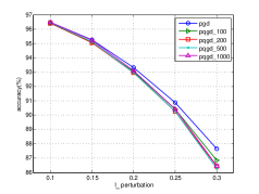
The effect of maximum allowed perturbations on the performance of gradient quantization on the MNIST dataset is shown in Figure 3(a). Here we test PGD and PQGD on an adversarial trained MNIST model. The results show that when maximum allowed perturbation is small, i.e., 0.1/1.0 $\ell_{\infty}$ perturbation, PGD and PQGD with various $b$ achieve similar accuracy on the adversarial trained MNIST model. When maximum allowed perturbation increases, PQGD with various $b$ is sharper than PGD. Consequently, when the maximum allowed perturbation is sufficiently large, i.e., 0.3/1.0 $\ell_{\infty}$ perturbation, PQGD with several choices of $b$ outperforms PGD by a small margin.

The effect of the maximum allowed perturbation on the performance of the gradient quantization on the Fashion-MNIST dataset (Fig.3(b)). For the Fashion-MNIST dataset, we obtain a similar outcome to the MNIST dataset. Specifically, PQGD with different $b$ outperforms PGD for all maximum allowed $\ell_{\infty}$ perturbations ranging from 0.1/1.0 to 0.2/1.0.

We conclude that when the maximum allowed perturbation is small, PQGD achieves comparable performance as PGD, as demonstrated in the results of Figure 3 and Table 6. In contrast when the maximum allowed perturbation increases, PQGD creates a sharper attack than PGD. Therefore, gradient quantization is more effective when the maximum allowed perturbation is larger.

4.4 Effect Of Number Of Steps On Gradient Quantization

We plot the average accuracy of five independent runs of PQGD and PGD, with different steps on the MNIST and Fashion-MNIST dataset (Fig. 4). Specifically, we test PQGD and PGD under a 0.3/1.0 $\ell_{\infty}$ maximum allowed perturbation on the adversarial trained MNIST model while we test approaches under a 0.2/1.0 $\ell_{\infty}$ maximum allowed perturbation on the adversarial trained Fashion-MNIST model.

(a) MNIST

(b) Fashion-MNIST

Figure 4: Effect of the number of steps on the averaged accuracy when applying PQGD and PGD attacks on adversarial trained models

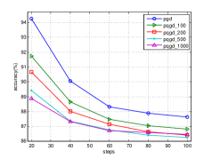
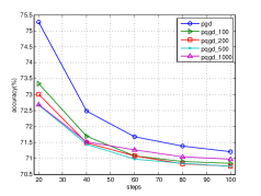
As shown in Figures 4(a) and 4(b), PQGD outperforms PGD with each choice of $b$ and for every number of steps ranging from 20 to 100. Interestingly, PQGD produces a much sharper attack than PGD when number of steps is small, e.g., 20 steps. It verifies our pervious claim that quantized gradients make use of the relative magnitude to boost the efficiency of crafting adversarial examples.

In the MNIST dataset, PQGD with $b=1000$ achieves an average accuracy of $88.89\%$ on our adversarial trained MNIST model while PGD reaches an average accuracy of $94.26\%$ when number of steps is $20$. PGD produces similar performance results to PQGD at step $20$, when the number of steps increases to $60$. In the Fashion-MNIST dataset, we observe similar effects of number of steps on the performance of PQGD. When the number of steps is fixed to $20$, PQGD with $b=500$ has an average accuracy of $72.68\%$ on the adversarial trained Fashion-MNIST model, while PGD has an averaged accuracy of $75.27\%$.

(a) 8.0/255.0

(b) 16.0/255.0

Figure 5: Effect of the number of steps on the accuracy of applying PQGD and PGD attacks on adversarial trained Cifar10 models under different allowed perturbations

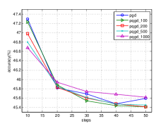
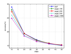
Figure 5 shows the effects of the number of steps on the performance of PQGD and PGD on the adversarial trained Cifar10 model from the Madry lab under $\ell_{\infty}$ allowed perturbations of $8.0/255.0$ and $16.0/255.0$. Under both allowed perturbations, PQGD performs better than PGD when number of steps is small, which is consistent with the result of MNIST and Fashion-MNIST datasets.

When the number of steps is $10$, under $8.0/255.0$ $\ell_{\infty}$ allowed perturbation, PQGD with $b=1000$ achieves an accuracy of $46.68\%$ on the adversarial trained Cifar10 model, while PGD has an accuracy of $47.3\%$. On the other hand, under $16.0/255.0$ $\ell_{\infty}$ allowed perturbation, PQGD with $b=1000$ has an accuracy of $24.91\%$ on the adversarial trained Cifar10 model, while PGD has an accuracy of $28.98\%$.

As the number of steps increases, the advantage of PQGD decreases compared with PGD. When the step number increases to $40$, PQGD and PGD demonstrate a similar performance on the adversarial trained Cifar10 model.

4.5 Choice of Hyperparameter $b$

The only hyperparameter we need to tune in our approach is $b$. We test PQGD and BLOB_QG with a wide spectrum of $b$. In previous sections, we only present part of results because of the space constraint. We observe that on each dataset for small $b$, i.e. $b<100$, attacks with quantized gradients exhibit limited improvement over their sign gradients. When $b$ is moderate, i.e., $100\leq b\leq 1000$, gradient quantization achieves the best performance. Therefore we present results when $b=100,200,500$ and $1000$ in previous sections. When $b$ is sufficiently large, i.e.,$b>1000$, attacks with quantized gradients gain advantage when the step size is small (Fig. 4 and 5). However when step number increases, the accuracy of attacks saturates at a relatively high level, and it will sometimes performs even worse than the vanilla PGD and DAA-BLOB approach.

5 Related Works

White-box Attack: Recall the definition of the white-box attack where the attacker has complete access to the underlying classifier information, including network architecture and parameters, training data and labels, even the defense mechanism deployed by the underlying system.

One of the earliest white-box attacks is FGSM[7], which is used to show the linear nature of DNN causes the vulnerability of DNN to adversarial examples. While FGSM is an attack based on $\ell_{\infty}$ distance, [16] introduced an attack under $\ell_{0}$ distance known as Jacobian-based Saliency Map Attack (JSMA). C&W attack [4] is introduced as an attack which can be applied under $\ell_{0}$, $\ell_{2}$ and $\ell_{\infty}$ distances. It is shown to significantly outperform FGSM and JSMA under the corresponding distance metrics. Research by [21] shows a surprising observation whereby adversarial training with single step attack such as FGSM leads to a degenerate global minimum. They resolved the issue by using attacks crafted from different neural networks. PGD is the universal first-order adversary [13], and a DNN model trained with PGD is supposed to be robust to any first-order attack.

Our work is an extension of PGD. We replace the sign gradient in each iteration of PGD with quantized gradients. PQGD and BLOB_QG belong to the category of white-box attacks because it has access to the network parameters and architecture, training data and its corresponding label.

Adversarial Training  Adversarial training was first introduced in [7] and [13] who formally define it through a lens of modified empirical risk minimization (Eq. 1). Evidence in [2] have shown that adversarial training is a state-of-the-art approach to increase the robustness of a model against adversarial examples.

Other Defenses Gradient masking is a defense that causes the target network to generate corrupted gradients [16]. Existing literatures including Thermometer Encoding [3], Input Transformation [9], stochastic activation pruning [5] Pre-Input Randomization Layer [24] PixelDefend [19], and Defense Distillation [17] fall into this category. Research by [2] shows that there are inherent limitations of these approaches and these defenses can be bypassed using more elaborated attack.

6 Conclusion

In this work, we revisit sign gradients, which are widely used in the white-box attacks, e.g., FGSM, PGD and DAA-BLOB. We argue that existing first-order attacks with sign gradients discards the information of relative magnitude between components in the raw gradient and thus affects the process of crafting effective adversarial examples. We propose quantized gradients to preserve the relative magnitude between components of raw gradients and we integrate existing first order attacks with them. Experiments show that iterative first order attacks with quantized gradients outperforms the attacks with sign gradients.

References

- [1] Dan Alistarh, Demjan Grubic, Jerry Li, Ryota Tomioka, and Milan Vojnovic. QSGD: communication-efficient SGD via gradient quantization and encoding. In Advances in Neural Information Processing Systems 30: Annual Conference on Neural Information Processing Systems 2017, 4-9 December 2017, Long Beach, CA, USA, pages 1707–1718, 2017.
- [2] Anish Athalye, Nicholas Carlini, and David A. Wagner. Obfuscated gradients give a false sense of security: Circumventing defenses to adversarial examples. In Proceedings of the 35th International Conference on Machine Learning, ICML 2018, Stockholmsmässan, Stockholm, Sweden, July 10-15, 2018, pages 274–283, 2018.
- [3] Jacob Buckman, Aurko Roy, Colin Raffel, and Ian J. Goodfellow. Thermometer encoding: One hot way to resist adversarial examples. In 6th International Conference on Learning Representations, ICLR 2018, Vancouver, BC, Canada, April 30 - May 3, 2018, Conference Track Proceedings, 2018.
- [4] Nicholas Carlini and David A. Wagner. Towards evaluating the robustness of neural networks. In 2017 IEEE Symposium on Security and Privacy, SP 2017, San Jose, CA, USA, May 22-26, 2017, pages 39–57, 2017.
- [5] Guneet S. Dhillon, Kamyar Azizzadenesheli, Zachary C. Lipton, Jeremy Bernstein, Jean Kossaifi, Aran Khanna, and Animashree Anandkumar. Stochastic activation pruning for robust adversarial defense. In 6th International Conference on Learning Representations, ICLR 2018, Vancouver, BC, Canada, April 30 - May 3, 2018, Conference Track Proceedings, 2018.
- [6] Ivan Evtimov, Kevin Eykholt, Earlence Fernandes, Tadayoshi Kohno, Bo Li, Atul Prakash, Amir Rahmati, and Dawn Song. Robust physical-world attacks on machine learning models. CoRR, abs/1707.08945, 2017.
- [7] Ian J. Goodfellow, Jonathon Shlens, and Christian Szegedy. Explaining and harnessing adversarial examples. In 3rd International Conference on Learning Representations, ICLR 2015, San Diego, CA, USA, May 7-9, 2015, Conference Track Proceedings, 2015.
- [8] Sven Gowal, Jonathan Uesato, Chongli Qin, Po-Sen Huang, Timothy Mann, and Pushmeet Kohli. An alternative surrogate loss for pgd-based adversarial testing. arXiv preprint arXiv:1910.09338, 2019.
- [9] Chuan Guo, Mayank Rana, Moustapha Cissé, and Laurens van der Maaten. Countering adversarial images using input transformations. In 6th International Conference on Learning Representations, ICLR 2018, Vancouver, BC, Canada, April 30 - May 3, 2018, Conference Track Proceedings, 2018.
- [10] Alex Krizhevsky and Geoffrey Hinton. Learning multiple layers of features from tiny images. Technical report, Citeseer, 2009.
- [11] Alexey Kurakin, Ian J. Goodfellow, and Samy Bengio. Adversarial machine learning at scale. In 5th International Conference on Learning Representations, ICLR 2017, Toulon, France, April 24-26, 2017, Conference Track Proceedings, 2017.
- [12] Yann LeCun, Léon Bottou, Yoshua Bengio, Patrick Haffner, et al. Gradient-based learning applied to document recognition. Proceedings of the IEEE, 86(11):2278–2324, 1998.
- [13] Aleksander Madry, Aleksandar Makelov, Ludwig Schmidt, Dimitris Tsipras, and Adrian Vladu. Towards deep learning models resistant to adversarial attacks. In 6th International Conference on Learning Representations, ICLR 2018, Vancouver, BC, Canada, April 30 - May 3, 2018, Conference Track Proceedings, 2018.
- [14] Nicolas Papernot, Patrick D. McDaniel, and Ian J. Goodfellow. Transferability in machine learning: from phenomena to black-box attacks using adversarial samples. CoRR, abs/1605.07277, 2016.
- [15] Nicolas Papernot, Patrick D. McDaniel, Ian J. Goodfellow, Somesh Jha, Z. Berkay Celik, and Ananthram Swami. Practical black-box attacks against machine learning. In Proceedings of the 2017 ACM on Asia Conference on Computer and Communications Security, AsiaCCS 2017, Abu Dhabi, United Arab Emirates, April 2-6, 2017, pages 506–519, 2017.
- [16] Nicolas Papernot, Patrick D. McDaniel, Somesh Jha, Matt Fredrikson, Z. Berkay Celik, and Ananthram Swami. The limitations of deep learning in adversarial settings. In IEEE European Symposium on Security and Privacy, EuroS&P 2016, Saarbrücken, Germany, March 21-24, 2016, pages 372–387, 2016.
- [17] Nicolas Papernot, Patrick D. McDaniel, Xi Wu, Somesh Jha, and Ananthram Swami. Distillation as a defense to adversarial perturbations against deep neural networks. In IEEE Symposium on Security and Privacy, SP 2016, San Jose, CA, USA, May 22-26, 2016, pages 582–597, 2016.
- [18] Mahmood Sharif, Sruti Bhagavatula, Lujo Bauer, and Michael K. Reiter. Accessorize to a crime: Real and stealthy attacks on state-of-the-art face recognition. In Proceedings of the 2016 ACM SIGSAC Conference on Computer and Communications Security, Vienna, Austria, October 24-28, 2016, pages 1528–1540, 2016.
- [19] Yang Song, Taesup Kim, Sebastian Nowozin, Stefano Ermon, and Nate Kushman. Pixeldefend: Leveraging generative models to understand and defend against adversarial examples. In 6th International Conference on Learning Representations, ICLR 2018, Vancouver, BC, Canada, April 30 - May 3, 2018, Conference Track Proceedings, 2018.
- [20] Christian Szegedy, Wojciech Zaremba, Ilya Sutskever, Joan Bruna, Dumitru Erhan, Ian J. Goodfellow, and Rob Fergus. Intriguing properties of neural networks. In 2nd International Conference on Learning Representations, ICLR 2014, Banff, AB, Canada, April 14-16, 2014, Conference Track Proceedings, 2014.
- [21] Florian Tramèr, Alexey Kurakin, Nicolas Papernot, Ian J. Goodfellow, Dan Boneh, and Patrick D. McDaniel. Ensemble adversarial training: Attacks and defenses. In 6th International Conference on Learning Representations, ICLR 2018, Vancouver, BC, Canada, April 30 - May 3, 2018, Conference Track Proceedings, 2018.
- [22] Shiqi Wang, Yizheng Chen, Ahmed Abdou, and Suman Jana. Mixtrain: Scalable training of formally robust neural networks. CoRR, abs/1811.02625, 2018.
- [23] Han Xiao, Kashif Rasul, and Roland Vollgraf. Fashion-mnist: a novel image dataset for benchmarking machine learning algorithms. arXiv preprint arXiv:1708.07747, 2017.
- [24] Cihang Xie, Jianyu Wang, Zhishuai Zhang, Zhou Ren, and Alan L. Yuille. Mitigating adversarial effects through randomization. In 6th International Conference on Learning Representations, ICLR 2018, Vancouver, BC, Canada, April 30 - May 3, 2018, Conference Track Proceedings, 2018.
- [25] Tianhang Zheng, Changyou Chen, and Kui Ren. Distributionally adversarial attack. CoRR, abs/1808.05537, 2018.