Lane Boundary Geometry Extraction from Satellite Imagery

Abstract.

Automated driving is becoming a reality where HD Map plays an important role in path planning and vehicle localization. Lane boundary geometry is one of the key components of HD Map. It is typically created from ground level LiDAR and imagery data, which have their limitations such as prohibitive cost, infrequent update, traffic occlusions, and incomplete coverage. In this paper, we propose a novel method to automatically extract lane information from satellite imagery using pixel-wise segmentation, which addresses the aforementioned limitations. We will also publish a dataset consists of satellite imagery and the corresponding lane boundaries as ground truth to train, test, and evaluate our method.

1. Introduction and Motivation

Highly accurate, precise, and detailed lane-level maps, as described in Open Lane Model by the Navigation Data Standard (Standard, 2016), is critical in enhancing driving safety and empowering automated driving. Lane-level maps enhances vehicle sensor functionality for contextual analysis of the environment, assist vehicle in executing controlled maneuvers beyond sensing range, and provide precise vehicle positioning and orientation on HD Maps. It works in conjunction with signs, barriers, poles, and surface markings to provide the vehicle a more comprehensive and accurate knowledge of the environment. One of the most important attribute in lane-level maps is lane boundary and geometry. Given millions of kilometers of roads in the world, it is cost-prohibitive and time-consuming to manually create and maintain such lane information at a centimeter-level. Ground-level imagery and LiDAR are two of the primary data sources to automatically extract lane information (Hillel et al., 2014).  (Broggi and Berte, 1995) proposed the method to detect roads from airborne imagery using color and edge information;   (Yang et al., 2013; Pazhayampallil and Kuan, 2013; Huval et al., 2015) proposed to detect road surface and lane markings from LiDAR using the highly accurate and precise 3D measurements in a LiDAR point cloud. Moreover, point cloud aligned with perspective imagery can generate training data (Gu et al., 2015) to assist lane-marking detection in perspective imagery. Object occlusion is one of the biggest challenge of road/lane extraction in both LIDAR point cloud and ground-level imagery. As an example, in Figure 1, a truck that drives along side the data acquisition vehicle at a similar speed casts a ”wall” in the middle of the road.

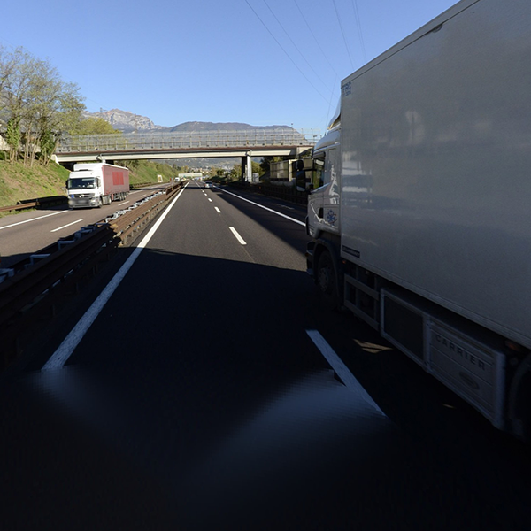
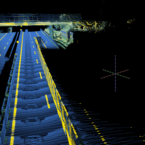
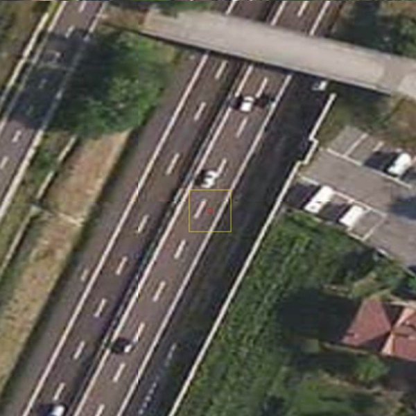
(a)	(b)	(c)

Figure 1. Object occlusion in perspective view (a), a wall caused by occlusion in LIDAR point cloud (b), and satellite image (c).

Recently, a lot of work has been done to automate lane-level map generation using vehicle-sensor meta data crowd-sourced from large fleet of vehicles (Chen and ZHUKOV, 2016) in addition to ground level data such as imagery (Chen et al., 2014; Chen and Yang, 2015; Chen, 2015), LiDAR (ZAVODNY and Chen, 2016), GPS, and Inertial Measurement Unit(IMU) collected by mobile mapping vehicles.

Extracting road/lane information from airborne imagery has its advantage over terrestrial data due to its comprehensive coverage, low-cost, ease to update. The history of road extraction from orthogonal imagery (e.g. satellite and aerial) can be traced back to more than forty years ago; however, limited by image resolution (typically over 2 meters per pixel), traditional approaches rely on edge detection, color segmentation, linear feature detection, and topological linking (Trinder and Wang, 1998; Bajcsy and Tavakoli, 1976) to extract road networks from overhead imagery. In recent years, more machine-learning based approaches are proposed to detect patch/pixel-wise road region (Mnih and Hinton, 2010; Heitz and Koller, 2008; Chaudhuri et al., 2012; Mokhtarzade and Zoej, 2007; Hu et al., 2007). These road centric approaches still cannot model the lane-level features even though the common satellite image resolution has improved to 0.5 meter per pixel.

Now, satellite imagery can have a resolution of 0.5 meter per pixel or less, which allows us to utilize the classic approaches with much detailed imagery to model lane-level features (Mattyus et al., 2015; Máttyus et al., 2016; Seo et al., 2012; Pink and Stiller, 2010). There are still two challenges after the lane boundary line is successfully detected: the representation of the lane model and the evaluation metric of model accuracy and performance. In paper (Pink and Stiller, 2010), the road model is represented as a collection of unstructured lines without attributes; while in paper (Seo et al., 2012), the definition of accuracy is based on the percentage of pixel-wise overlap comparing to their manually drawn line masks in the input images. Hence, their claimed accuracy is less persuasive.

Autonomous vehicles are becoming more of a reality. The increasing demand of HD mapping can be predicted, especially for interstate transportation (i.e. autonomous truck (Freedman, 2017). The three largest highway networks in the world, U.S., China, and India, are $103$, $446$, and $79$ thousand kilometers (Administration, 2013; Technology, 2014) long, respectively, which motivates us to concentrate on highway-level road network in this paper. We propose a novel, automated lane boundary extraction technique from satellite imagery. Our approach consists of two stages: pixel-wise line segmentation and hypotheses-grouping classification linking. The pixel-wise line segmentation approach contains patch-based lane-marking classification, and for each positive patch, we segment line pixels to generate line candidates. Hypotheses-linking connects each line candidate by minimizing the proposed cost function to generate structured lane model. A formalized road-model-accuracy-metric is designed to evaluate the results rigorously. We also manually extracted lane boundary ground truth from our dataset. Along with satellite imagery, it can be used for training, testing, and evaluation for comparative studies.

2. Methodology

Our lane-boundary-geometry extraction approach contains two stages. In training, similar to (Gu et al., 2015), we use the ground truth lane boundary geometry and the corresponding satellite imagery from Bing Tile Server as input, project lane boundary lines to imagery, crop image into small patches, and train our patch level classifier. In extraction, our approach uses pre-trained classifier, target route/trajectory, and corresponding satellite imagery as input, detects patch-level lane marking candidates (Costea and Leordeanu, 2016), segment the pixel-wise lane marking candidates, and links (Seo et al., 2012) the pixel-wise candidates to generate lane boundary geometry.

2.1. Patch and Patch Level Classification

The objective of this step is to build a classifier that can determine whether an image patch contains any lane marking pixel. Even though the ground truth road model is organized in chunk-wise structure , due to the specificity of the tile system, generating training patches in chunks unnecessarily queries the image server twice (each tile always contains two to three chunks at high resolution level). Hence, our solution is designed as tile-wise - for each tile along trajectory, project all control points of each functional line and connect them. To reduce noise (i.e. lane marking pixel of adjacent road surfaces), the surface region is bounded by road boundaries (given in the ground truth dataset). Samples contain lane marking pixels in red and road surface region in green are illustrated in Figure 2.

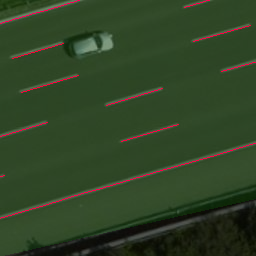
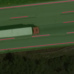
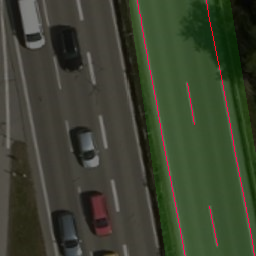
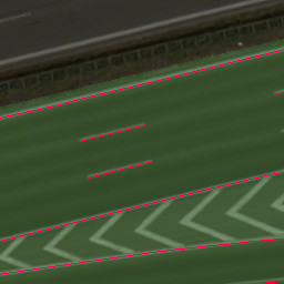
Figure 2. Satellite tile images fused with ground truth lane boundary geometry at tile pixel $[557869,363521]$, $[557909,363513]$, $[558036,363507]$ and $[557879,363518]$ at level $20$ from left to right. Road region highlighted in green, bounded by road boundaries. Lane marking highlighted in red.

A sliding window is designed to crop training patches from corresponding satellite image within the road surface. The label for each patch is determined by whether there is any lane marking pixel hit in the current patch. To reduce misleading ground truth patches (the patch contains two independent lines), an appropriate window size should be thinner than lane width in real scale, which is $3.5$ meters . In this project, the ground resolution is approximately $0.15$ meter per pixel at tile level $20$, which means the patch size should be less than $24$. Examples of positive (contain lane marking pixel) and negative patches are shown in Figure 3.

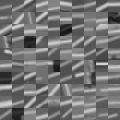
(a)	(b)

Figure 3. 100 sample patches of original orientation lane-marking patches (a) and non-lane-marking patches (b).

Given a satellite tile image (shown in Figure 4 (a)), its corresponding probability map of patch level lane marking with certain configuration (patch size is $12$ pixels, use pixel representation feature and Random Forest classifier) is illustrated in Figure 4 (b).

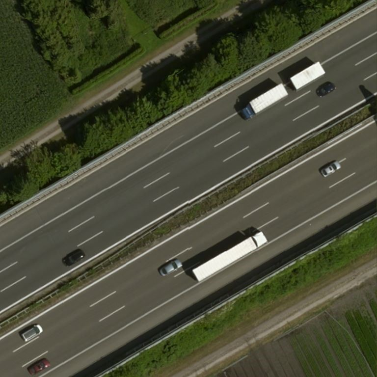
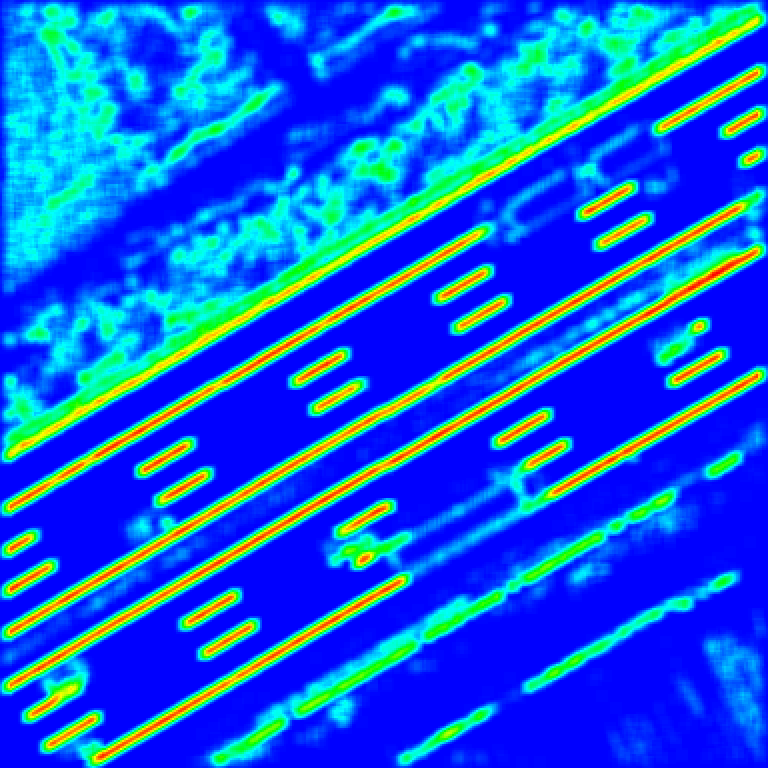
(a) (b)

Figure 4. Original satellite tile image (a) and its patch level lane marking probability map (b) at location $48.2203\degree,11.5126\degree$.

2.2. Pixel-wise Lane Marking Segmentation

Our patch level classification returns a probability map as output, which contains high probability lane marking regions like the red area shown in Figure 4(b). However, since each region is always several pixels wide (depending on patch size and step length), this wide range obviously could not meet the requirement considering the definition of HD Maps (Bittel et al., 2015).

To segment and locate precise lane marking pixels, we consider pixels with the highest intensity in each slice of lane marking region perpendicular to road trajectory as lane-marking candidate. Then, we fit a line segment through the lane marking pixel candidates. For example, in Figure 5, assuming the trajectory is up, for each row of this region, the highest intensity points are $151$, $154$, and $150$, respectively, which means the lane marking line segment should be the centerline of this region.

Even though the satellite image resolution has already matched the lane marking width, limited by image compression, hardware constraints(lens, CMOS), and optical limitations (i.e. angular resolution), tiny/thin object will always be blurred at its boundaries when captured. Furthermore, to segment more precise lane marking pixel locations, we introduce sub pixel-wise segmentation. For each slice of the lane marking region, fit a Gaussian model (green lines in Figure 5) and find the peak of each model (yellow circles in Figure 5). Then, the lane marking pixel location becomes sub-pixel-wise instead of the naive pixel-wise of each slice of the lane marking region. Theoretically, line accuracy can be improved by at most half a pixel. The pixel-wise lane marking segmentation result is illustrated in Figure 6.

Figure 5. Pixel-wise and sub pixel-wise lane marking segmentation visualization, each number inside pixel represents its intensity value converted from the raw RGB image.

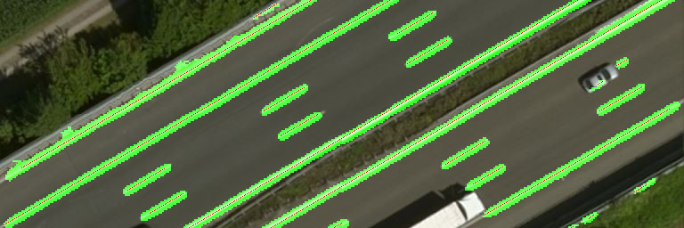
Figure 6. Lane marking region candidates (green regions) and pixel-wise lane marking pixel candidates (red dots) overview (top) and zoom view (bottom).

2.3. Line Candidates Grouping, Classification and Linking

The previous step generates unstructured line segments without relative position and function label (solid/dashed line). Because of occlusion (i.e. trees, vehicles, buildings, and their shadows) and poorly painted lane markings(examples shown in Figure 7 (a)), less true lane marking lines will be detected, while more misleading lines (false positive) will be detected if lane-marking-like objects appear (i.e. guardrail, curb, wall shown in Figure 7 (b)).

(a)
(b)

Figure 7. Phenomenons cause mis-detection: bad painting quality and shadow (a), misleading objects that cause false positive: high reflective metal guardrail and cement curb (b).

The method of of transforming the unstructured lines to structured lines with function labels contains three steps: grouping line candidates from each chunk, classify the function of each line group, and link the missing lines.

In the grouping step, whether or not to push a line into a group depends on the relative distance between the current line to all other line candidates in the current chunk, in the neighboring chunk(s), and their relative distances to road centerline/vehicle trajectory. For example, line candidates (gray) from four continuous chunks and vehicle trajectory (blue dashed) are illustrated in Figure 8 (a). After the grouping step, five groups are generated and colored in Figure 8 (b). On a certain portion of the road, for each group, the function label is determined by the ratio of the total length of detected line segments belong to this group, to the total length of road contains this line group. Typically, consider reasonable mis-detection and wrong detection, the length ratio of dashed line is below $40\%$ and the ratio of solid line is above $80\%$. In the task of modeling highway roads, there is an assumption that each road portion can have at most two solid lines bounding the (drivable) road surface. Figure 8 (c) illustrates the groups after the classification step, solid lines and dashed lines are colored in dark red and dark green, respectively, lines out of solid lines (drivable road surface) are colored in gray and will be ignored. In the final step, if one chunk does not contain a line that belongs to the group which passes this chunk, a synthetic line will be interpolated (light green lines shown in Figure 8 (d)).

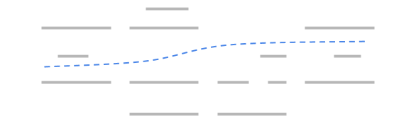
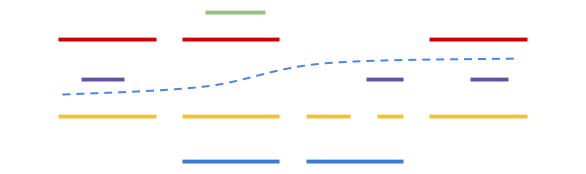
(a)	(b)
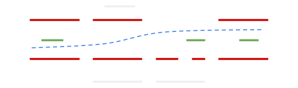
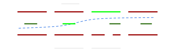
(c)	(d)

Figure 8. Illustrations of Line Candidates grouping, classification and linking steps.

Notice that in this grouping, classification, and linking procedure, numerous thresholds and constrains (i.e. distance threshold, search range, etc.) are needed to control the process. Generally speaking, if we abstract all these variables into one degree: loose (longer search range, wider distance threshold) and tight (shorter search range, narrower distance threshold) to reflect the abstract performance of the model, the tightness-to-performance chart is illustrated in Figure 9. As we can see, it is a trade off between function accuracy and geometry accuracy .

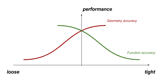
Figure 9. Constrains tightness to modeling performance chart.

Furthermore, if any constraint (additional information) is provided when extracting the lane boundary geometry - for example, if we know the number of lanes for a certain portion of the road - this process can be fine tuned to generate a much better result.

3. Lane Boundary Ground Truth Collection

In paper (Seo et al., 2012), the author uses manually-drew, pixel-based ground truth, represented in ’mask’ format (Seo, 2012), to evaluate his accuracy. The author does not have detailed description and statistic of his dataset. The number of ground truth masks is 50, which also limits its persuasion.

To code our lane boundary geometry dataset, we built an interactive tool which allows us to manually draw lane boundaries from scratch and present background image from various sources (i.e. point cloud projection, satellite imagery, etc.). The user interface is shown in Figure 11. An lane boundary geometry extraction from LiDAR point cloud pipeline will be executed at the very beginning to generate near-perfect lane boundaries to boost our modeling efficiency from $29.2$ meters per minute to $12.8$ meters per minute. Then we use our tool to edit (delete, move, insert, etc.) the control points on lane boundary lines to make align them with the background imagery perfectly.

As one of the contributions, we will publish this line based lane boundary geometry ground truth on our FTP server once the paper is accepted. In this section, we are going to discuss the road selection, coding rules, lane boundary geometry representation, and potential system errors. More lane boundary geometry data of diversified scenarios (luminance condition, country, etc.) will be published as future work.

3.1. Lane Boundary Data Description

We collect lane boundary geometry on Germany Autobahn A99 (Bundesautobahn 99), from location $48.2206\degree 11.5153\degree$ to $48.2057\degree 11.4586\degree$, divided into seven portions (five for training and two for testing) to exclude overpass structures and other unexpected scenarios.

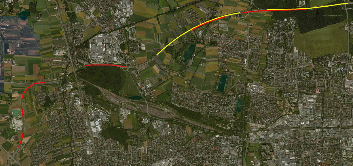
Figure 10. Illustration of our ground truth portions highlighted on aerial imagery, red for training and yellow for testing.

This dataset contains training data (approximately $10.14$ kilometers) and testing data ($6.07$ kilometers), which follows similar coding rules but two key differences in coding the dashed line and the coordinate system due to the particularity of this research. In training set (coverage shown in Figure 10, highlighted in red), dashed lines are represented as isolated line segments (two end points), shown in Figure 11(b), and aligned with satellite imagery coordinates. In testing dataset (coverage shown in Figure 10, highlighted in yellow), dashed lane markings belong to one set of continuous/sequential control points if they are semantically treated as one line and aligned with point cloud, as shown in Figure 11(c). All control points are placed right in the middle of their corresponding lane marking.

Also, in this dataset, we code road boundaries (i.e. guardrail, curb) and use them to separate road surface from non-road surface (to exclude lane-marking like objects outside the road surface).

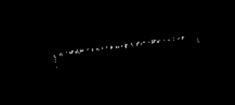
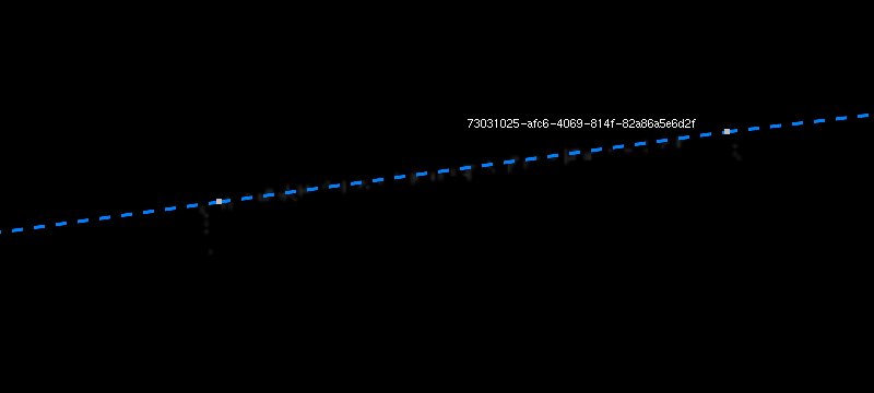
(a)	(b)
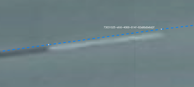
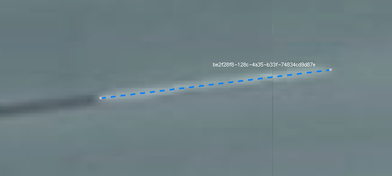
(c)	(d)

Figure 11. Lane boundary line in point cloud view (a), test lane boundary line (continuous dashed line) in point cloud view (b), test lane boundary line in satellite imagery mode (misalignment between two systems can be obtained)(c) and train lane boundary line (isolated dashed line) in satellite imagery view (d). UUID denotes the line id.

3.2. Data Annotation

To represent lane boundary geometry and lane boundary lines for user convenience, lane boundary lines are evenly divided into $12$-meter chunks. Each chunk is wrapped up in a single JSON file that follows this structure:

Chunk JSON file id: INT map version: INT lines: line id: STRING: UUID type: STRING: [’solid’/’dashed’/’trajectory’] points: FLOAT: [n by (latitude, longitude)] matrix

3.3. Errors in latitude, longitude, and altitude

Aerial imagery and point cloud are stored/represented in two coordinate systems - Mercator projection coordinate system (Bing, 2012) and Cartesian coordinate system (Atanacio-Jiménez et al., 2011; Schwarz, 2010) - because of their acquisition techniques. Aerial image tile system is designed by demand years ago, but it inevitably has heavy distortion.

To avoid distortion, point cloud processing procedures and our labeling tool are designed to process data in Cartesian coordinate system. The different coordinate systems lead to a slight distance error when coded on these two layers - point cloud representation in a Cartesian local tangent plane: North-East-Up (NEU) and imagery represented in Mercator projection. Assume location $[\phi,\lambda,0]$ at zoom level $l$, the Euclidean distance $d_{p}(\phi,\lambda,d_{x},d_{y})$ between the points back-projected through Mercator projection and Cartesian coordinate transformations of pixel shift $d_{x},d_{y}$ is complicated.

After simplification, $d_{p}$ can be represented as the function of latitude $\phi$, pixel shift $[d_{x},dy]$, and zoom level $l$, and the illustration of function $d_{p}(\phi,d_{x},d_{y},l)$ at certain zoom level $l=20$ and certain $dy=0$ is shown in Figure 12. According to precision requirements from most ’HD’ definitions (HERE, 2015; TomTom, 2015; TMTpost, 2016), the error caused by fusion of two coordinate systems (less than $5$ cm all around the world at tile level $20$) does not have an impact on the final accuracy.

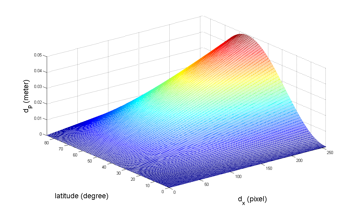
Figure 12. Illustration of $d_{p}(\phi,d_{x},d_{y},l)$ when $l=20$ and $d_{y}=0$.

4. Experiments

In the proposed methodology, we test numerous patch configurations (patch feature, size) and machine learning techniques to find the appropriate classifier and run our end-to-end program to extract lane boundary geometry using this optimum classifier. In this section, we are going to present both patch level accuracy and final extracted model accuracy by using the metrics described in the next sub-section.

4.1. Accuracy Definition

Lane boundaries is a collection of numeric and functional polylines/splines in control point representation (Schindler et al., 2012), we cannot simply report the accuracy in pixel-wise representation as (Seo et al., 2012) proposes.

Considering the features of lane boundary and the misalignment between ground truth and modeling coordinates, we propose two metrics for a persuasive performance score: function level and geometry level accuracy. Theoretically, the misalignment between two coordinates causes transformation from one model to another to shift, scale, rotate, and even skew. In our task, scaling, rotating, and skewness are unnoticeable so they can be ignored, only shift transformation will be considered.

Given ground truth lines $L_{i}=\{l_{i,1},l_{i,2},....,l_{i,n}\}$ and predicted lines $L^{\prime}_{i}=\{l^{\prime}_{i,1},l^{\prime}_{i,2},....,l^{\prime}_{i,m}\}$ from $i$th chunk, the first step is to match $l\in L_{i}$ and $l^{\prime}\in L^{\prime}_{i}$. Let $d(l,l^{\prime})$ denotes the distance between pair lines $l$ and $l^{\prime}$ with sign (for example, left for negative) and $Pair(l_{i},L^{\prime}_{i})$ denotes the paired line in $L^{\prime}_{i}$ of $l_{i}$. Align two models by using each $l_{i}$ and each $l^{\prime}_{i}$, find the

$$\operatorname{argmin}_{all\>pairs}(\sum_{l_{i,j}\in L_{i}}(d(l_{i,j},Pair(l_{i,j},L^{\prime}_{i}))))$$

Figure 13 shows two pairs: green dashed arrow and red dashed arrow. By comparing the total length of the green and red solid arrows, the best match is green dashed arrow. Given distance threshold $T_{d}$ from requirement (for example, HD Maps), a correct detection of $l^{\prime}_{i}$ and $l_{i}$ is counted if their functions are matched and $d(l^{\prime}_{i},l_{i})<T_{d}$. Then, the accuracy of the predicted model compared to ground truth can be represented in

$$\operatorname{\textit{precision}}_{\operatorname{function}}=\frac{number\>of\>correct\>detections}{(\parallel\textbf{L}\parallel)}$$

$$\operatorname{\textit{recall}}_{\operatorname{function}}=\frac{number\>of\>correct\>detections}{(\parallel\textbf{L}^{\prime}\parallel)}$$

$$\textbf{L}=\{L_{i}\},\textbf{L}^{\prime}=\{L^{\prime}_{i}\},i\in road$$

To calculate geometry accuracy, for each pair $\{l_{i,j}:Pair(l_{i,j},L^{\prime}_{i})\}$ in $L_{i}$, the $\operatorname{\textit{shift}}$ is defined as $AVG_{i}(d(l_{i}:Pair(l_{i,j},L^{\prime}_{i}))),L^{\prime}_{i}\>and\>L_{i}\in\textbf{L}$, and the $\operatorname{\textit{performance}}_{geometry}$ is defined as $AVG_{i}(1-\frac{\sigma(d(l_{i}:Pair(l_{i,j},L^{\prime}_{i})))}{\sigma_{max}(\parallel L_{i}\parallel)})$, while $\sigma_{max}=\sigma(L_{max})$ is used to normalized precision for each chunk, where $L_{max}=M\cup N$, set $M$ contains $\operatorname{\textit{floor}}(\frac{\parallel L_{i}\parallel)}{2})$’s $T_{d}$ and set $N$ contains $\operatorname{\textit{ceiling}}(\frac{\parallel L_{i}\parallel)}{2})$’s $-T_{d}$ (for example, if $\parallel L_{i}\parallel)$ equals $4$, then $\sigma_{max}(\parallel L_{i}\parallel)=\sigma([T_{d},T_{d},-T_{d},-T_{d}])$). With this $\{\operatorname{\textit{perfomance}}:\operatorname{\textit{shift}}\}$ metric, we can present the lane boundary geometry reasonably if the alignment between two source coordinates is unknown. Also, we can tweak the parameters of end-to-end program to generate expected model depends on the project requirement. For example, if alignment is not a requirement and we want to address the LiDAR shadow issue from point cloud, we would need to tweak the configurations with the lowest performance.

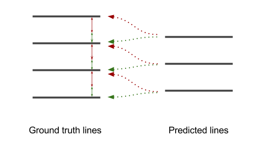
Figure 13. Ground truth lane boundary lines (left) and predicted lane boundary lines (road) pairing.

4.2. Patch level accuracy

To find the best patch level classifier, we crop tile image with given ground truth data as described in Section 2.1, with configurable variables such as as patch size ($8,12,16,24$), patch feature (pixel representation and gradient based features such as Histogram of Oriented Gradients (HOG), Local Binary Pattern (LBP)), and numerous machine learning techniques (Random Forest (RF), Support Vector Machine (SVM), Artificial Neural Network (ANN) and Convolutional Neural Network (CNN)) to evaluate their precision and recall. Figure 14 shows the performances of different training configurations of $10$-fold Cross Validation.

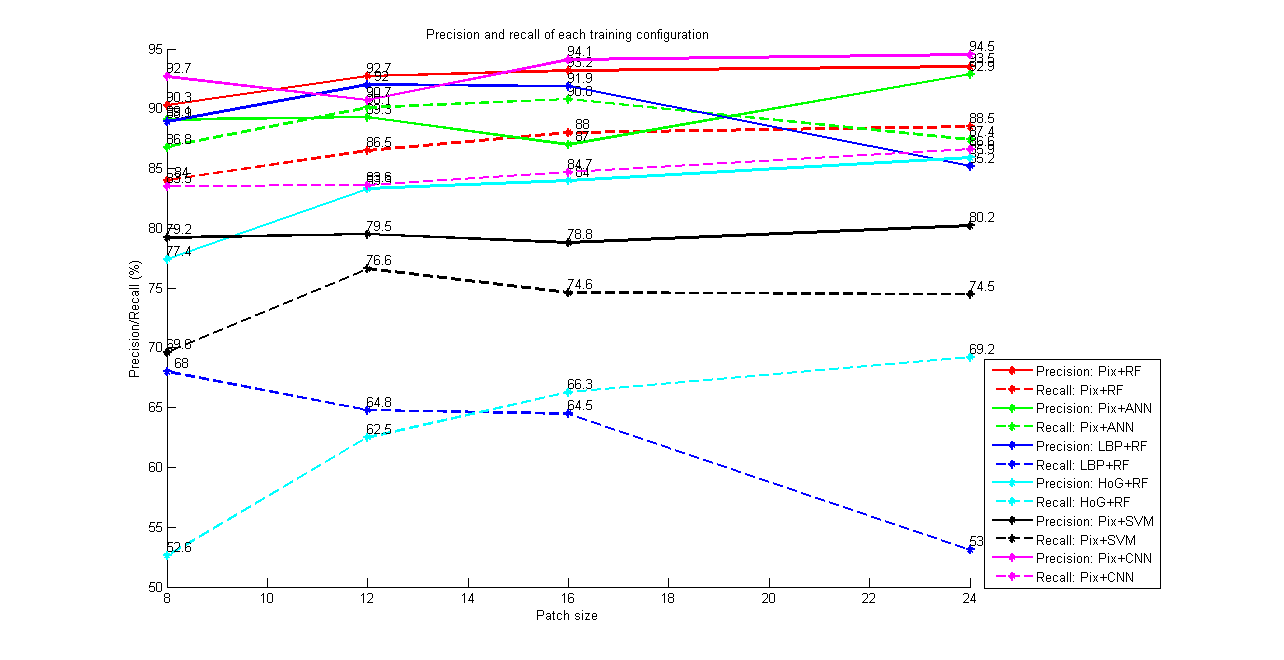
Figure 14. Patch level precision and recall of each training configuration.

According to our evaluation result, the change in patch size does not have a big impact on patch level performance. Considering the computational cost, a patch size of $12$ is used in our final patch level classifier to generate a dense/smooth lane marking probability map shown in Figure 4 (b).

4.3. Lane Boundary Geometry Accuracy

With the pre-trained classifier and our end-to-end solution, we tweaked parameters and thresholds as mentioned in Section 2.3 to evaluate the performance of our approach on the testing set. The function level and geometry performances are shown in Table 1 below.

Table 1. Model level performance with different conditions.

Sample of ground truth lane boundaries and final extracted lane boundaries rendered on satellite imagery is shown in Figure 15 (a). Each chunk is bounded by blue rectangle, yellow stars denote road trajectory, ground truth model is rendered in red, and the resulting lane boundary geometry is rendered in green.

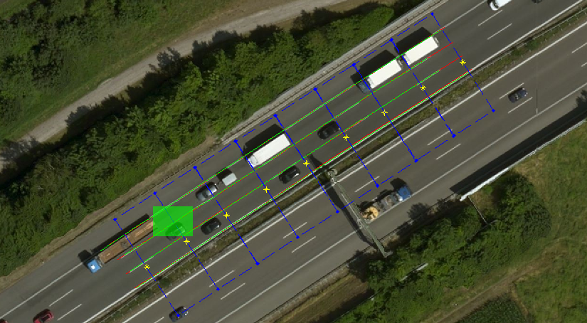
Figure 15. Result visualization overview (top) and zoom view of the green box (bottom).

The shift from experiment result shows the misalignment between ground truth coordinate (from point cloud) and testing data coordinate (from satellite imagery) is negligible on testing data, which was also validated by our observation. Benefited from the above-average conditions of the testing road (good painting quality, light traffic), the extracted lane boundaries achieved impressive results when measured against the ground truth before and after the linking stage at geometry level. Function level precision improves $10.83\%$ by the linking stage while geometry level performance only dropped $1.63\%$ due to the interpolated, synthetic lane boundaries. Even though the median error of the results is lower than $5$ cm, limited by original satellite imagery resolution, we can claim that our lane boundary geometry accuracy is $30$ cm .

5. Concluding Remarks and Future Directions

In this paper we present a novel approach to automatically extract lane boundary geometry from reasonably high resolution satellite imagery. It complements the existing ground-level based methods with advantages such as cost-effectiveness, wider coverage, and better updatability. We also designed a comprehensive lane boundary geometry evaluation metric and published our lane boundary geometry dataset.

The following areas will be investigated for further improvement:

1. Elevation information is not available in satellite imagery. This can be solved with additional data source such as DEM and the High Definition Digital Elevation Model (HD DEM) database (Zang et al., 2017).

2. We will combine both ground level and airborne data to extract lane boundary geometry. Alignment of these two data sets is critical for the fusion. Some feature points visible in both model could register the two data sets. For example, road surface markings and pole like objects are good control point candidates.

3. By adding absolute/relative spatial information to each pixel (Pinheiro and Collobert, 2014), a machine learning based (especially Recurrent Convolutional Neural Networks) lane marking pixel classification may substitute the approach of combining machine learning based lane marking patch classification and pixel-wise segmentation proposed in this paper.

4. Other than limited access roads such as highway and expressway, there is a large number of urban road networks that also need to be modeled in high definition for fully automated driving. Occlusions and shadows of urban roads in satellite imagery make it very challenging to apply our approach. In addition, the complex geometry and topology of urban road may require a different lane model for automation.

References

- (1)
- Administration (2013) Federal Highway Administration. 2013. Highway Statistics 2013. (2013). https://www.fhwa.dot.gov/policyinformation/statistics/2013/hm220.cfm
- Atanacio-Jiménez et al. (2011) Gerardo Atanacio-Jiménez, José-Joel González-Barbosa, Juan B Hurtado-Ramos, Francisco J Ornelas-Rodríguez, Hugo Jiménez-Hernández, Teresa García-Ramirez, and Ricardo González-Barbosa. 2011. LIDAR velodyne HDL-64E calibration using pattern planes. International Journal of Advanced Robotic Systems 8, 5 (2011), 59.
- Bajcsy and Tavakoli (1976) Ruzena Bajcsy and Mohamad Tavakoli. 1976. Computer recognition of roads from satellite pictures. IEEE Transactions on Systems, Man, and Cybernetics 9 (1976), 623–637.
- Bing (2012) Bing. 2012. Bing Maps Tile System. (2012). https://msdn.microsoft.com/en-us/library/bb259689.aspx
- Bittel et al. (2015) Sebastian Bittel, Vitali Kaiser, Marvin Teichmann, and Martin Thoma. 2015. Pixel-wise segmentation of street with neural networks. arXiv preprint arXiv:1511.00513 (2015).
- Broggi and Berte (1995) Alberto Broggi and Simona Berte. 1995. Vision-based road detection in automotive systems: A real-time expectation-driven approach. Journal of Artificial Intelligence Research 3 (1995), 325–348.
- Chaudhuri et al. (2012) D Chaudhuri, NK Kushwaha, and A Samal. 2012. Semi-automated road detection from high resolution satellite images by directional morphological enhancement and segmentation techniques. IEEE journal of selected topics in applied earth observations and remote sensing 5, 5 (2012), 1538–1544.
- Chen (2015) X. Chen. 2015. Detecting common geographic features in images based on invariant components. (Sept. 8 2015). https://www.google.com/patents/US9129163 US Patent 9,129,163.
- Chen et al. (2014) X. Chen, R.B. Hui, and N. Alwar. 2014. Determining a geometric parameter from a single image. (Nov. 25 2014). https://www.google.com/patents/US8896686 US Patent 8,896,686.
- Chen and Yang (2015) X. Chen and X. Yang. 2015. Detecting ground geographic features in images based on invariant components. (Feb. 10 2015). https://www.google.com/patents/US8953838 US Patent 8,953,838.
- Chen and ZHUKOV (2016) X. Chen and V. ZHUKOV. 2016. Detecting road condition changes from probe data. (June 7 2016). https://www.google.com/patents/US9361797 US Patent 9,361,797.
- Costea and Leordeanu (2016) Dragos Costea and Marius Leordeanu. 2016. Aerial image geolocalization from recognition and matching of roads and intersections. arXiv preprint arXiv:1605.08323 (2016).
- Freedman (2017) David Freedman. 2017. 10 Breakthrough Technologies. MIT Technology Review.
- Gu et al. (2015) Xiaodong Gu, Andi Zang, Xinyu Huang, Alade Tokuta, and Xin Chen. 2015. Fusion of color images and LiDAR data for lane classification. In Proceedings of the 23rd SIGSPATIAL International Conference on Advances in Geographic Information Systems. ACM, 69.
- Heitz and Koller (2008) Geremy Heitz and Daphne Koller. 2008. Learning spatial context: Using stuff to find things. In European conference on computer vision. Springer, 30–43.
- HERE (2015) HERE. 2015. HERE introduces HD maps for highly automated vehicle testing. (2015). http://360.here.com/2015/07/20/here-introduces-hd-maps-for-highly-automated-vehicle-testing/
- Hillel et al. (2014) Aharon Bar Hillel, Ronen Lerner, Dan Levi, and Guy Raz. 2014. Recent progress in road and lane detection: a survey. Machine vision and applications 25, 3 (2014), 727–745.
- Hu et al. (2007) Jiuxiang Hu, Anshuman Razdan, John C Femiani, Ming Cui, and Peter Wonka. 2007. Road network extraction and intersection detection from aerial images by tracking road footprints. IEEE Transactions on Geoscience and Remote Sensing 45, 12 (2007), 4144–4157.
- Huval et al. (2015) Brody Huval, Tao Wang, Sameep Tandon, Jeff Kiske, Will Song, Joel Pazhayampallil, Mykhaylo Andriluka, Pranav Rajpurkar, Toki Migimatsu, Royce Cheng-Yue, and others. 2015. An empirical evaluation of deep learning on highway driving. arXiv preprint arXiv:1504.01716 (2015).
- Mattyus et al. (2015) Gellert Mattyus, Shenlong Wang, Sanja Fidler, and Raquel Urtasun. 2015. Enhancing Road Maps by Parsing Aerial Images Around the World. In Proceedings of the IEEE International Conference on Computer Vision. 1689–1697.
- Máttyus et al. (2016) Gellért Máttyus, Shenlong Wang, Sanja Fidler, and Raquel Urtasun. 2016. HD Maps: Fine-grained Road Segmentation by Parsing Ground and Aerial Images. In Proceedings of the IEEE Conference on Computer Vision and Pattern Recognition. 3611–3619.
- Mnih and Hinton (2010) Volodymyr Mnih and Geoffrey E Hinton. 2010. Learning to detect roads in high-resolution aerial images. In European Conference on Computer Vision. Springer, 210–223.
- Mokhtarzade and Zoej (2007) Mehdi Mokhtarzade and MJ Valadan Zoej. 2007. Road detection from high-resolution satellite images using artificial neural networks. International journal of applied earth observation and geoinformation 9, 1 (2007), 32–40.
- Pazhayampallil and Kuan (2013) Joel Pazhayampallil and Kai Yuan Kuan. 2013. Deep Learning Lane Detection for Autonomous Vehicle Localization. (2013).
- Pinheiro and Collobert (2014) Pedro Pinheiro and Ronan Collobert. 2014. Recurrent convolutional neural networks for scene labeling. In International Conference on Machine Learning. 82–90.
- Pink and Stiller (2010) Oliver Pink and Christoph Stiller. 2010. Automated map generation from aerial images for precise vehicle localization. In Intelligent Transportation Systems (ITSC), 2010 13th International IEEE Conference on. IEEE, 1517–1522.
- Schindler et al. (2012) Andreas Schindler, Georg Maier, and Florian Janda. 2012. Generation of high precision digital maps using circular arc splines. In Intelligent Vehicles Symposium (IV), 2012 IEEE. IEEE, 246–251.
- Schwarz (2010) Brent Schwarz. 2010. LIDAR: Mapping the world in 3D. Nature Photonics 4, 7 (2010), 429.
- Seo (2012) Young-Woo Seo. 2012. Augmenting cartographic resources and assessing roadway state for vehicle navigation. Carnegie Mellon University.
- Seo et al. (2012) Young-Woo Seo, Chris Urmson, and David Wettergreen. 2012. Ortho-image analysis for producing lane-level highway maps. In Proceedings of the 20th International Conference on Advances in Geographic Information Systems. ACM, 506–509.
- Standard (2016) Navigation Data Standard. 2016. Navigation Data Standard - Open Lane Model Documentation. Technical Report. Navigation Data Standard.
- Technology (2014) Roadtraffic Technology. 2014. The world’s biggest road networks. (2014). http://www.roadtraffic-technology.com/features/featurethe-worlds-biggest-road-networks-4159235/
- TMTpost (2016) TMTpost. 2016. Baidu Driverless Cars Run In Wuzhen, Powered By Four Leading Technologies. (2016). https://medium.com/@TMTpost/baidu-driverless-cars-run-in-wuzhen-poweredby-four-leading-technologies-tmtpost-53c0b3072cec
- TomTom (2015) TomTom. 2015. HD MAP - HIGHLY ACCURATE BORDER-TO-BORDER MODEL OF THE ROAD. (2015). http://automotive.tomtom.com/uploads/assets/972/1474451229-hd-map-product-info-sheet.pdf
- Trinder and Wang (1998) John C Trinder and Yandong Wang. 1998. Automatic road extraction from aerial images. Digital Signal Processing 8, 4 (1998), 215–224.
- Yang et al. (2013) Bisheng Yang, Lina Fang, and Jonathan Li. 2013. Semi-automated extraction and delineation of 3D roads of street scene from mobile laser scanning point clouds. ISPRS Journal of Photogrammetry and Remote Sensing 79 (2013), 80–93.
- Zang et al. (2017) Andi Zang, Xin Chen, and Goce Trajcevski. 2017. High-Definition Digital Elevation Model System (Vision Paper). In Proceedings of International Conference on Scientific and Statistical Database Management. ACM.
- ZAVODNY and Chen (2016) A.G. ZAVODNY and X. Chen. 2016. Method and apparatus for processing and aligning data point clouds. (Aug. 23 2016). https://www.google.com/patents/US9424672 US Patent 9,424,672.