Small sample corrections for Wald tests in Latent Variable Models

Abstract

Latent variable models (LVMs) are commonly used in psychology and increasingly used for analyzing brain imaging data. Such studies typically involve a small number of participants ($n$<100), where standard asymptotic results often fail to appropriately control the type 1 error. This paper presents two corrections improving the control of the type 1 error of Wald tests in LVMs estimated using maximum likelihood (ML). First, we derive a correction for the bias of the ML estimator of the variance parameters. This enables us to estimate corrected standard errors for model parameters and corrected Wald statistics. Second, we use a Student’s $t$-distribution instead of a Gaussian distribution to account for the variability of the variance estimator. The degrees of freedom of the Student’s $t$-distributions are estimated using a Satterthwaite approximation. A simulation study based on data from two published brain imaging studies demonstrates that combining these two corrections provides superior control of the type 1 error rate compared to the uncorrected Wald test, despite being conservative for some parameters. The proposed methods are implemented in the R package lavaSearch2 available at https://cran.r-project.org/web/packages/lavaSearch2.

keywords: latent variable models, maximum likelihood, repeated measurements, small sample inference, Wald test.

1 Introduction

Understanding brain mechanisms is essential to improve prevention and treatment of brain disorders. For instance, it has been hypothesized that the serotonin system is a key factor in major depressive disorders (MDD) and most antidepressants attempt to act on this system. Unfortunately, less than half of the patients respond to first-line antidepressant treatment. A deeper understanding of the serotonin brain system is therefore needed. While it is not yet possible to non-invasively measure the extracellular level of serotonin in the brain, medical imaging allows one to simultaneously visualize the brain structure (using Magnetic Resonance Imaging - MRI) and quantify the binding potential of certain serotonin receptors (using Positron Emission Tomography - PET), e.g. see Figure 1.

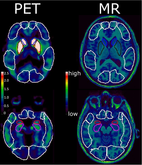
Figure 1: Single-subject serotonin 4 receptor binding and five regions of interest (ROI): amygdala (red areas), caudate (blue), hippocampus (purple), neocortex (white) and putamen (black). Images at left show ROIs overlaid on a brain image depicting voxel-level serotonin 4 receptor binding (color scale units, serotonin 4 receptor binding). Images at right show the same regions overlaid on a high-resolution structural MR image, for spatial orientation.

Recently, Latent variable models (LVMs) have been used to identify the brain serotonin level from the binding potentials measured in several brain regions and relate this level to patient group, test performance, or genotype status (Fisher et al., (2015), Fisher et al., (2017), Stenbæk et al., (2017), Deen et al., (2017), Perfalk et al., (2017), da Cunha-Bang et al., (2018)). These models were estimated by maximum likelihood (ML) and statistical inference was most often performed based on the asymptotic distribution of Wald statistics. However, the sample size in these studies is rather limited (respectively 68, 144, 24, 34, 41, 43), especially in light of the number of parameters required to obtain a satisfying model fit (respectively 29, 29, 48, 31, 37, 40). The application of asymptotic results is thus questionable, e.g., one may be worried that the type 1 error is not at its nominal level. This has been shown using simulation studies for the global fit tests (i.e., likelihood ratio test, Herzog et al., (2007)), for which corrections have been proposed (Satorra and Bentler,, 1994; Bentler and Yuan,, 1999; Wu and Lin,, 2016; Jiang and Yuan,, 2017; Maydeu-Olivares,, 2017). To our knowledge, the small sample properties of the Wald test in LVMs has not been carefully studied and software packages for LVMs, such as the R package lavaan (Rosseel,, 2012) or Mplus (Muthén and Muthén,, 2017), implement several small sample corrections for the global fit tests, but no corrections for the Wald tests.

Current solutions for small sample inference include profile likelihood (Pek and Wu,, 2015), the use of resampling procedures: bootstrap, permutation, jackknife, or the use of Bayesian techniques such as Monte Carlo Markov Chains (MCMC). The main drawback of these methods is that they are computationally intensive. In addition, each method has specific pros and cons. For instance, bootstrap and jackknife may not appropriately control the type 1 error rate because they rely on asymptotic results, e.g., Parr, (1983) and Carpenter and Bithell, (2000). Although permutation procedures appropriately control the type 1 error rate, they can test only very specific combinations of the model parameters. McNeish, (2016) have shown that MCMC is highly sensitive to the specification of the prior distributions of the parameters in small samples and may, therefore, not be straightforward to use. In this article we focus on LVMs estimated by ML and propose an analytical approach to approximate the distribution of the Wald statistics. This approach does not require any user input nor any additional model fit. It modifies the usual asymptotic distribution of the Wald statistic in two ways, similar to the correction proposed by Kenward and Roger, (1997) for mixed models: (i) correcting the bias of the ML-estimator for variance parameters and (ii) modeling the distribution of the Wald statistics using Student’s $t$-distributions instead of Gaussian distributions.

The remainder of the article is structured as follows: we formally introduce LVMs and discuss the validity of the traditional testing procedure in section 2. In section 3, we illustrate the use of LVM and the inflated type 1 error rate of the traditional testing procedure in three applications. Our small sample correction is presented in sections 4 and 5. They, respectively, extend (i) and (ii) when testing a single hypothesis in LVMs. Extension to multiple hypotheses and robust standard errors are discussed in section 6. The control of the type 1 error rate after correction is assessed in section 7 using simulations studies inspired from the three applications. These are re-analyzed with the proposed correction in section 8. We end the article with a discussion. The proposed correction is implemented in an R package called lavaSearch2, available on CRAN (https://cran.r-project.org/web/packages/lavaSearch2). An overview of the functionnalities and code examples can be found in the vignette of the package. The code used for the simulation studies and for the illustrations is available at https://github.com/bozenne/Article-lvm-small-sample-inference.

2 Inference in linear LVMs

We consider a sample of $n$ independent and identically distributed (iid) replicates $(\boldsymbol{Y}_{i},\boldsymbol{X}_{i})_{i\in\{1,\ldots,n\}}$ generated by $m$ endogenous random variables $\boldsymbol{Y}=(Y_{1},\dots,Y_{m})$ and $l$ exogenous random variables $\boldsymbol{X}=(X_{1},\dots,X_{l})$. A LVM is defined by a measurement model linking the endogenous variables to a set of latent variables $\boldsymbol{\eta}$ and to the exogenous variables:

$$\boldsymbol{Y}_{i} =\boldsymbol{\nu}+\boldsymbol{\eta}_{i}\Lambda+\boldsymbol{X}_{i}K+\boldsymbol{\varepsilon}_{i}\text{, where }\boldsymbol{\varepsilon}_{i}\sim\mathcal{N}\left(0,\Sigma_{\varepsilon}\right)$$ (1)

and by a structural model relating the latent variables to the exogenous variables:

$$\boldsymbol{\eta}_{i} =\boldsymbol{\alpha}+\boldsymbol{\eta}_{i}B+\boldsymbol{X}_{i}\Gamma+\boldsymbol{\zeta}_{i}\text{, where }\boldsymbol{\zeta}_{i}\sim\mathcal{N}\left(0,\Sigma_{\zeta}\right)$$ (2)

where $B$ is a matrix with 0 on its diagonal and such that $1-B$ is invertible. We denote by $p$ the number of parameters, by $\boldsymbol{\theta}$ the vector containing the model parameters (we use the bold notation to denote row vectors), and by $\mathcal{S}_{\boldsymbol{\theta}}$ the set of model parameters. The conditional distribution of $\boldsymbol{Y}$ given $\boldsymbol{X}$ follows from equations (1) and (2):

$$\boldsymbol{Y}_{i}|\boldsymbol{X}_{i}\sim\mathcal{N}\left(\boldsymbol{\mu}(\boldsymbol{\theta},\boldsymbol{X}_{i}),\Omega(\boldsymbol{\theta})\right)$$

where $$\boldsymbol{\mu}(\boldsymbol{\theta},\boldsymbol{X}_{i})=\boldsymbol{\nu}+\boldsymbol{\alpha}(1-B)^{-1}\Lambda+\boldsymbol{X}_{i}\Gamma(1-B)^{-1}\Lambda+\boldsymbol{X}_{i}K$$

and $$\Omega(\boldsymbol{\theta})={\Lambda}^{\intercal}(1-B)^{-\intercal}\Sigma_{\zeta}(1-B)^{-1}\Lambda+\Sigma_{\varepsilon}$$ (3)

The parameters can either be involved in the conditional mean, both in the conditional mean and variance, or only in the conditional variance. Parameters of the first type, i.e., parameters $\boldsymbol{\nu}$, $\boldsymbol{\alpha}$, $K$ and $\Gamma$, will be called mean parameters and denoted $\boldsymbol{\theta}_{\mu}$. Parameters satisfying the latter type, i.e., parameters in $\Sigma_{\varepsilon}$ and $\Sigma_{\zeta}$, will be called variance parameters and denoted $\boldsymbol{\theta}_{\Sigma}$. Estimation can be carried out using ML, see Holst and Budtz-Jørgensen, (2013) for more details. ML is known to give asymptotically unbiased, efficient and normally distributed estimates. For a given parameter $\theta\in\mathcal{S}_{\boldsymbol{\theta}}$, we can use a Wald statistic:

$$t_{\theta}=\frac{\hat{\theta}}{\sigma_{\hat{\theta}}}$$ (4)

to assess whether $\theta=0$. Under the null hypothesis, $t_{\theta}$ is asymptotically normally distributed with mean 0 and variance 1. Here $\hat{\theta}$ denotes the value of $\theta$ estimated using ML and $\sigma_{\hat{\theta}}$ is the standard deviation of the estimator (the variance-covariance matrix of the estimator of $\boldsymbol{\theta}$ will be denoted $\Sigma_{\boldsymbol{\hat{\theta}}}$). In most applications $\sigma_{\hat{\theta}}$ is not known but we can plug the ML estimate of the standard error, $\hat{\sigma}_{\hat{\theta}}$, in equation (4) to obtain a tractable test statistic:

$$\hat{t}_{\theta}=\frac{\hat{\theta}}{\hat{\sigma}_{\hat{\theta}}}$$ (5)

This has two consequences in finite samples: (i) the variance of $\hat{t}_{\theta}$ will typically be greater than 1 and (ii) $\hat{t}_{\theta}$ may not be normally distributed due to the variability of $\hat{\sigma}_{\hat{\theta}}$. Indeed, if $\hat{\sigma}^{2}_{\hat{\theta}}$ follows a $\chi^{2}$ distribution and is independent of $\hat{\theta}$, then $\hat{t}_{\theta}$ follows a Student’s $t$-distribution (up to a multiplicative factor). Regarding (i), using a first order Taylor expansion and taking the expectation, we can express the first order bias of $\hat{\sigma}_{\hat{\theta}}$:

$$\mathbb{E}\left[\hat{\sigma}_{\hat{\theta}}-\sigma_{\hat{\theta}}\right]=\mathbb{E}\left[\boldsymbol{\hat{\theta}}-\boldsymbol{\theta}\right]{\frac{\partial\sigma_{\hat{\theta}}}{\partial\boldsymbol{\theta}}}^{\intercal}+o_{p}(n^{-\frac{1}{2}})$$ (6)

In correctly specified models, $\sigma_{\hat{\theta}}$ can be consistently estimated using the appropriate element in the inverse of the expected information matrix (denoted $\mathcal{I}(\boldsymbol{\theta})$). As shown in supplementary material LABEL:SM-SM:Information, the expected information relative to the parameters $\theta$ and $\theta^{\prime}$ in a LVM can be expressed as:

$$\mathcal{I}(\theta,\theta^{\prime})= \frac{n}{2}tr\left(\Omega(\boldsymbol{\theta})^{-1}\frac{\partial\Omega(\boldsymbol{\theta})}{\partial\theta}\Omega(\boldsymbol{\theta})^{-1}\frac{\partial\Omega(\boldsymbol{\theta})}{\partial\theta^{\prime}}\right)+\sum_{i=1}^{n}\frac{\partial\boldsymbol{\mu}(\boldsymbol{\theta},\boldsymbol{X}_{i})}{\partial\theta}\Omega(\boldsymbol{\theta})^{-1}{\frac{\partial\boldsymbol{\mu}(\boldsymbol{\theta},\boldsymbol{X}_{i})}{\partial\theta^{\prime}}}^{\intercal}$$ (7)

Since $\sigma_{\hat{\theta}}$ is an element of the inverse of $\mathcal{I}(\boldsymbol{\theta})$, it depends on the variance parameters via $\Omega(\boldsymbol{\theta})$ so $\frac{\partial\sigma_{\hat{\theta}}}{\partial\boldsymbol{\theta}}$ is typically non-zero. In small samples, the ML estimator of the variance parameters is in general biased (Harville,, 1977); it follows that the first term of equation (6) is non-zero and $\hat{\sigma}_{\hat{\theta}}$ is biased in finite samples. We expect that the ML estimator of the variance parameters will be biased downward and $\sigma_{\hat{\theta}}$ will increase with the variance parameters, so $\hat{\sigma}_{\hat{\theta}}$ will be biased downward.

3 Applications to real data

We consider three applications involving simple to complex LVMs (see Figure 2 for the corresponding path diagrams). The first investigates the correspondance between mixed models and LVMs and the next two were chosen from the studies on the serotonin system mentioned in the introduction. The latter two applications are representative of scientific questions encountered in that field: can we correlate a genetic variable to indirect measurements of the brain serotonin system? Can we study the relationship between indirect measurements of the brain serotonin system and indirect measurements of the cognitive ability of a subject?

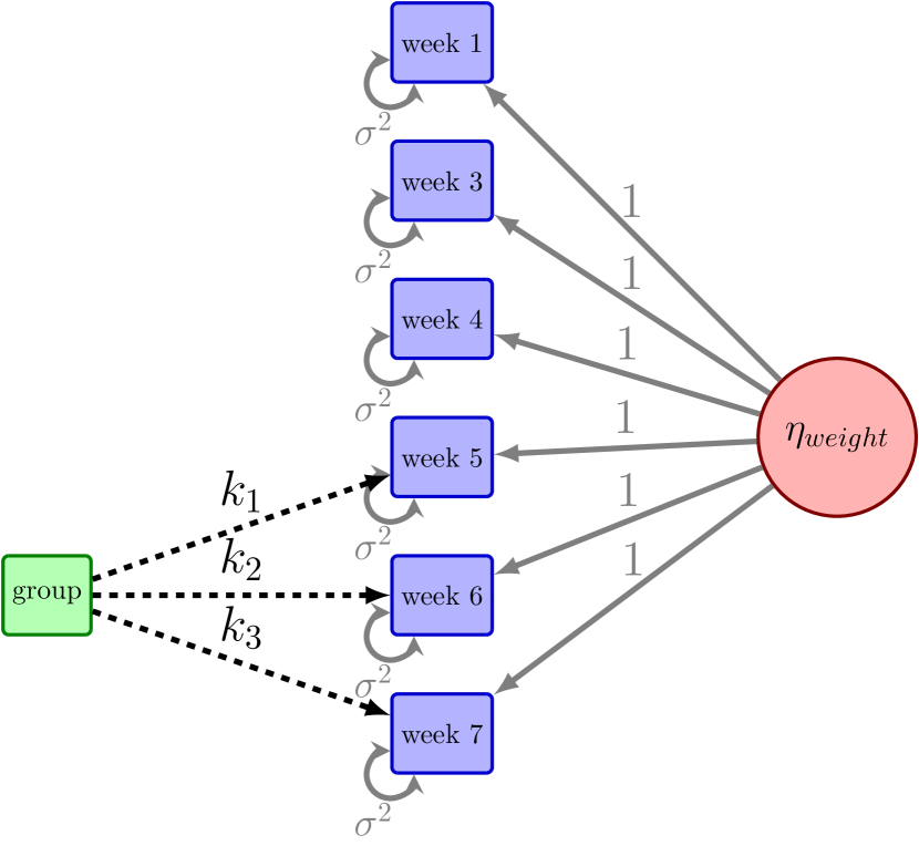
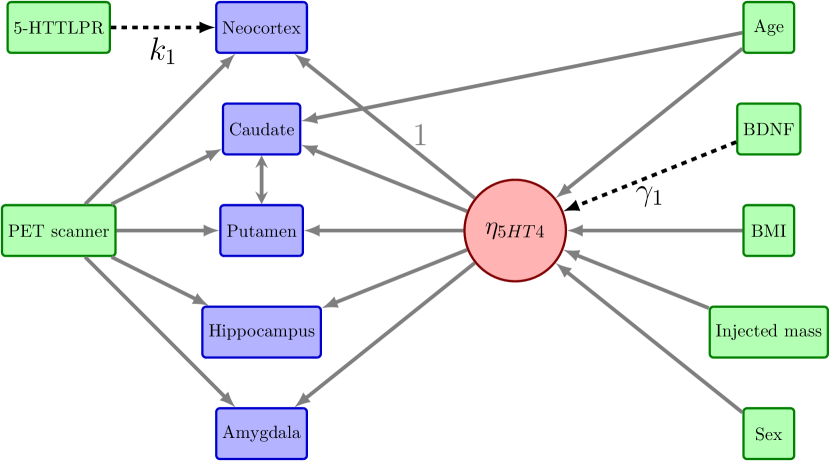
Application A : Growth of guinea pigs

Application B : serotonin 4 receptor and genetric polymorphisms (Fisher et al.,, 2015)

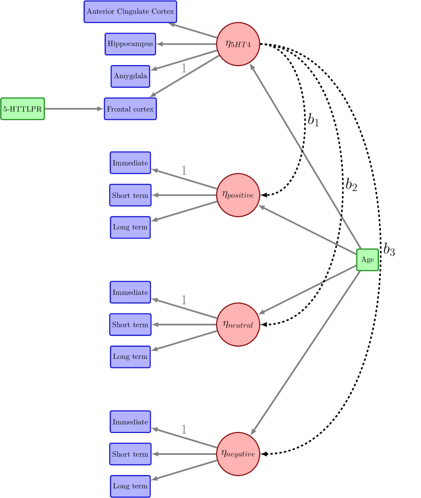
Application C : serotonin 4 receptor and verbal memory recall (Stenbæk et al.,, 2017)

Figure 2: Path diagram of the LVM associated with each application: the observed variables are displayed in blue (outcomes) and green (covariates) while the latent variable is displayed in red. The union of the full and dotted arrows represent the relationships between variables modeled by the LVM. The black dotted arrows denote the parameters of interest and symbols above the full arrows represent constraints, e.g., in 2Application B the residual variances are constrained to have the same value and the loadings to be 1.

Growth of guinea pigs (Application A): this application originates from a practical class on mixed models (http://publicifsv.sund.ku.dk/j̃ufo/RepeatedMeasures2017.html) where the students are asked to monitor the growth of two groups of guinea pigs over seven weeks using a random intercept model. One group of pigs received vitamin E at the beginning of week 5, while the other group serves as a control (see supplementary material LABEL:SM-SM:figPig for a graphical display of the data) so the treatment effect is only modeled from week 5 to 7 using a different parameter for each week. The dataset used is small: each group contains only five animals. The random intercept model is equivalent to a LVM where the loadings are set to 1 (i.e. $\Lambda=(\lambda_{1},\ldots,\lambda_{6})=(1,\ldots,1)$) and the residual variances are assumed constant over time:

$$Y_{it} =\left\{\begin{array}[]{cc}\nu_{t}+\eta_{i}+\varepsilon_{it}\text{, if }t<5\\ \nu_{t}+\eta_{i}+\text{group}_{i}k_{t-4}+\varepsilon_{it}\text{, if }t\geq 5\end{array}\right.\text{ where }\varepsilon_{it}\sim\mathcal{N}\left(0,\sigma^{2}\right)\text{ and }\eta_{i}\sim\mathcal{N}\left(0,\tau\right)$$

The corresponding path diagram is shown in the upper left panel of Figure 2.

The interest lies in assessing whether vitamin E affects the growth of the pigs. This can be performed by testing whether all treatment parameters are 0 (i.e. $k_{1}=k_{2}=k_{3}=0$) using a Wald test. In a mixed model, we obtained a Wald statistic of 4.25 and a p-value of 0.0102 while the Wald statistic of the LVM was 5.02 and the corresponding p-value was 0.00176. The large discrepancy is due to the fact that, in mixed models, restricted maximum likelihood (REML) is preferred over ML when estimating the model because it corrects the bias of the ML estimator of the variance parameters. Kenward and Roger, (1997) proposed an additional correction by modeling the distribution of the Wald statistic using a Student’s $t$-distribution and estimating its degrees of freedom by the method of moments. This has become the gold standard procedure in mixed models and is what has been used here. This correction is not available for LVM, leading, in this example, to an inflated type 1 error rate: 0.102 instead of 0.05, according to simulation studies.

Serotonin 4 receptor binding and genetic polymorphisms (Application B): Fisher et al., (2015) were interested in whether two genetic variants, i.e., BDNF val66met and 5-HTTLPR polymorphisms, were associated with brain serotonin levels. The authors collected genetic data and PET brain imaging data, using two scanners, from 68 healthy humans. The final dataset contained 73 observations because five participants were scanned twice. The serotonin 4 receptor binding, a proxy for brain serotonin levels, was computed in five brain regions (amygdala, caudate, hippocampus, neocortex and putamen). Preliminary regression analyses suggested an association between the BDNF val66met genotype and serotonin 4 receptor levels in all brain regions, whereas the effect of the 5-HTTLPR polymorphisms was found to be specific to only the neocortex region. Data were subsequently analyzed in a LVM where the regional serotonin 4 binding measurements were linked to a single latent variable, representing an unobservable brain serotonin level. This latent variable was affected by BDNF val66met genotype status to model a global effect ($\Gamma$ parameter), whereas the 5-HTTPLR effect was directly modeled on the neocortex region ($K$ parameter). Covariates assumed to affect the serotonin level were related to the latent variable. To remove systematic differences in serotonin measurements, a direct effect of the scanner on each brain region was modeled. The path diagram of the LVM is displayed in lower left panel of Figure 2. The LVM had 29 parameters.

Inference was performed using cluster robust standard errors, i.e., the score was computed at the participant level when using the sandwich estimator. The effects of the BDNF val66met and 5-HTTLPR polymorphisms were estimated to be, respectively, $\hat{\gamma}_{2}=0.074$ ($\text{p-value}=0.005$) and $\hat{k}_{1}=-0.073$ ($\text{p-value}=7.2\,10^{-6}$). In a LVM estimated under the constraint of no genetic effects as a generative model, a simulation study showed that the actual type 1 error rate was 0.074 for the effect of the BDNF val66met and 0.061 for the effect of the 5-HTTLPR polymorphisms.

Serotonin 4 receptor binding and verbal memory recall (Application C): Stenbæk et al., (2017) investigated the relationship between episodic memory and serotonin 4 receptor binding. They collected data from 24 healthy volunteers who underwent a PET scan and a verbal affective memory test (VAMT). PET and memory measures were acquired proximal to each other but not at the same time. In the VAMT test, subjects are asked to remember words immediately after having learned them (immediate memory), five minutes after (short term memory), and 30 minutes after (long term memory). Words were divided into three categories: positive, negative, and neutral valence words. The serotonin 4 receptor binding was measured in four brain regions known to be involved in affective processing and memory (amygdala, anterior cingulate cortex, frontal cortex and hippocampus). Four latent variables were constructed: three that combine the immediate, short term, and long term memory for each type of word and one that combines the serotonin 4 receptor binding across the brain regions (respectively, $\eta_{positive}$, $\eta_{neural}$, $\eta_{negative}$, and $\eta_{5HT4}$). Associations between the latent variables were adjusted for age. The path diagram of the LVM is shown in Figure 2 (right panel). The resulting LVM had 48 parameters.

With this LVM, they found an effect of the binding construct ($\eta_{5HT4}$) on the memory constructs ($\eta_{positive}$, $\eta_{neutral}$, $\eta_{negative}$) with, respectively, $\hat{b}_{1}=-7.3$ ($\text{p-value}=0.0005$), $\hat{b}_{2}=-6.7$ ($\text{p-value}=0.004$), and $\hat{b}_{3}=-3.7$ ($\text{p-value}=0.07$). Using a LVM estimated under the constraint of no relation between memory and serotonin 4 receptor binding, a simulation study found that the type 1 error was 0.063 for $b_{1}$, 0.085 for $b_{2}$, and 0.084 for $b_{3}$.

4 Bias correction for the ML-estimator of the variance parameters

We now develop a method to correct the small sample bias of the estimated variance parameters, $\boldsymbol{\hat{\theta}}_{\Sigma}$. Denoting the observed residuals by $\boldsymbol{\xi}_{i}(\boldsymbol{\hat{\theta}})=\boldsymbol{Y}_{i}-\boldsymbol{\mu}(\boldsymbol{\hat{\theta}},\boldsymbol{X}_{i})$, it is well known that in a standard linear model the variance of the observed residuals underestimates the (true) conditional variance of $Y$. We show in supplementary material LABEL:SM-SM:varResiduals that this result generalizes to LVMs. Indeed, given that $\mathbb{E}\left[{\boldsymbol{\xi}_{i}(\boldsymbol{\theta})}^{\intercal}\boldsymbol{\xi}_{i}(\boldsymbol{\theta})\right]=\Omega(\boldsymbol{\theta})$ and $\mathcal{I}(\boldsymbol{\theta})^{-1}=\Sigma_{\boldsymbol{\hat{\theta}}}$, the variance of the observed residuals can be decomposed into:

$$\mathbb{E}\left[{\boldsymbol{\xi}_{i}(\boldsymbol{\hat{\theta}})}^{\intercal}\boldsymbol{\xi}_{i}(\boldsymbol{\hat{\theta}})\right] =\Omega(\boldsymbol{\theta})-\Psi_{i}+o_{p}(n^{-1})\quad\text{ where }\Psi_{i}={\frac{\partial\boldsymbol{\mu}(\boldsymbol{\theta},\boldsymbol{X}_{i})}{\partial\boldsymbol{\theta}}}^{\intercal}\Sigma_{\boldsymbol{\hat{\theta}}}\frac{\partial\boldsymbol{\mu}(\boldsymbol{\theta},\boldsymbol{X}_{i})}{\partial\boldsymbol{\theta}}$$ (8)

Since the first order bias, $\Psi_{i}$, is positive definite, the variance of the observed residuals is a downward biased estimate of $\Omega(\boldsymbol{\theta})$. This result is similar to the one found by Kauermann and Carroll, (2001) for Generalized Estimating Equation models. Denoting $\Psi=\frac{1}{n}\sum_{i=1}^{n}\Psi_{i}$, we obtain by averaging over the samples:

$$\mathbb{E}\left[\frac{1}{n}\sum_{i=1}^{n}{\boldsymbol{\xi}_{i}(\boldsymbol{\hat{\theta}})}^{\intercal}\boldsymbol{\xi}_{i}(\boldsymbol{\hat{\theta}})\right]=\Omega(\boldsymbol{\theta})-\Psi+o_{p}(n^{-1})$$

Example (standard linear model): consider the generative mechanism $Y_{i}=\boldsymbol{X}_{i}\beta+\varepsilon_{i}$ with $\varepsilon_{i}\sim\mathcal{N}\left(0,\sigma^{2}\right)$, where $Y$ is a univariate endogenous variable, $\boldsymbol{X}$ contains $p$ exogenous variables and $\varepsilon_{i}$ are independent and identically normally distributed. As shown in supplementary material LABEL:SM-SM:LM-correctBias, formula (8) gives that $\Psi_{i}=\sigma^{2}\boldsymbol{X}_{i}\left({\boldsymbol{X}}^{\intercal}\boldsymbol{X}\right)^{-1}{\boldsymbol{X}}^{\intercal}_{i}$ and $\Psi=\frac{p}{n}\sigma^{2}$. Note that the first order bias of the ML estimator can be removed by considering the estimator $\left(\hat{\sigma}^{c}\right)^{2}=\hat{\sigma}^{2}+\hat{\Psi}=(1+\frac{p}{n})\hat{\sigma}^{2}$.

This example motivates the use of $\Psi$ to correct the small sample bias of the ML estimator. We only attempt to correct the bias of the variance parameters, $\boldsymbol{\theta}_{\Sigma}$, because simulation studies show a much smaller bias for the other parameters (e.g., see supplementary material LABEL:SM-SM:tableBiasML). To do so, we assume that $\Omega(\boldsymbol{\hat{\theta}})$ and $\mathbb{E}\left[\frac{1}{n}\sum_{i=1}^{n}{\boldsymbol{\xi}_{i}(\boldsymbol{\hat{\theta}})}^{\intercal}\boldsymbol{\xi}_{i}(\boldsymbol{\hat{\theta}})\right]$ have the same first order bias. Then, given $\Psi$, we can defined a corrected ML-estimator of $\Omega$: $\hat{\Omega}^{c}=\Omega(\boldsymbol{\hat{\theta}})+\Psi$. From equation (3) and considering $(\Lambda,B)$ fixed, we get that $\Omega(\boldsymbol{\theta})$ is linearly related to the variance parameters, so we can find a matrix $Z$ (depending only on $\Lambda$ and $B$) such that $vec(\hat{\Omega}^{c})=Z\,\boldsymbol{\theta}_{\Sigma}+\mathbf{r}$, where $\mathbf{r}$ is a possible residual error and $vec$ is the column stacking operator transforming $\hat{\Omega}^{c}$ into a vector. Given $Z$, we obtain a new estimate of $\boldsymbol{\theta}_{\Sigma}$ by solving the least squares problem. This leads to the following iterative procedure to estimate $\Psi$ and get bias-corrected estimates of $\boldsymbol{\theta}_{\Sigma}$ and $\mathcal{I}(\boldsymbol{\theta})$:

Initialize: $\hat{\mathcal{I}}^{(0)}\leftarrow\hat{\mathcal{I}}(\boldsymbol{\theta})$

for k=1 to $\infty$ do

       (i) Compute for each subject $i$ the bias $\hat{\Psi}_{i}^{(k)}$ by plugging $\left(\hat{\mathcal{I}}^{(k-1)}\right)^{-1}$ and $\frac{\partial\boldsymbol{\mu}(\boldsymbol{\hat{\theta}},\boldsymbol{X}_{i})}{\partial\boldsymbol{\theta}}$ into equation (8).

       [2mm] (ii) Compute the average bias $\hat{\Psi}^{(k)}=\frac{1}{n}\sum_{i=1}^{n}\hat{\Psi}_{i}^{(k)}$.

       [2mm] (iii) Estimate $\hat{\Omega}^{(k)}$ by $\Omega(\boldsymbol{\hat{\theta}})+\hat{\Psi}^{(k)}$.

       [2mm] (iv) Find $\boldsymbol{\hat{\theta}}_{\Sigma}^{(k)}$ satisfying $\hat{\Omega}^{(k)}={\hat{\Lambda}}^{\intercal}(1-\hat{B})^{-\intercal}\Sigma_{\zeta}\left(\boldsymbol{\hat{\theta}}_{\Sigma}^{(k)}\right)(1-\hat{B})^{-1}\hat{\Lambda}+\Sigma_{\varepsilon}\left(\boldsymbol{\hat{\theta}}_{\Sigma}^{(k)}\right)$.

       [2mm] (v) Compute the corrected derivatives $\frac{\partial\hat{\Omega}^{(k)}}{\partial\boldsymbol{\theta}}$ using $\boldsymbol{\hat{\theta}}_{\Sigma}^{(k)}$.

       [2mm] (vi) Compute $\hat{\mathcal{I}}^{(k)}$ by plugging $\hat{\Omega}^{(k)}$, $\frac{\partial\boldsymbol{\mu}(\boldsymbol{\hat{\theta}},\boldsymbol{X}_{i})}{\partial\boldsymbol{\theta}}$, and $\frac{\partial\hat{\Omega}^{(k)}}{\partial\boldsymbol{\theta}}$ into equation (7).

      

end for

Algorithm 1

In practice, the algorithm is stopped when the difference between two consecutive estimates of $\hat{\Omega}^{(k)}$ is small, e.g., in our software implementation we require that the Frobenius norm of the difference is smaller than $10^{-5}$. We can check that algorithm 1 gives a sequence of $\hat{\Psi}^{(k)}$ that are semi-definite positive. Indeed, if at step (i) $\hat{\mathcal{I}}^{(k-1)}$ is definite positive then $\hat{\Psi}^{(k)}_{i}$ is semi-definite positive. This in turn would imply that $\hat{\Psi}^{(k)}$ is semi-definite positive, $\hat{\Omega}^{(k)}$ is definite positive, and so is $\hat{\mathcal{I}}^{(k)}$. We obtain the stated property by induction. Showing the convergence and monotonicity of $\Psi^{(k)}$ is more difficult, so we only consider specific cases:

Example (standard linear model): supplementary material LABEL:SM-SM:LM-correctBias shows that the estimated bias of the residual variance at iteration $k$ is $\hat{\Psi}^{(k)}=\frac{p}{n}\left(\hat{\sigma}^{(k-1)}\right)^{2}$. The corresponding corrected residual variance is $\left(\hat{\sigma}^{(k)}\right)^{2}=\hat{\sigma}^{2}\sum_{\kappa=0}^{k}\frac{p^{\kappa}}{n^{\kappa}}\xrightarrow[k\rightarrow\infty]{}\frac{n}{n-p}\hat{\sigma}^{2}$. The corrected residual variance tends toward the usual unbiased estimate of $\sigma^{2}$. The convergence is fast, especially when $n$ is large, since there is a factor $\frac{p}{n}$ between the contribution of the current iteration and the contribution of the next iteration. The same applies to $\hat{\Psi}^{(k)}$. Note that $\hat{\Psi}^{(k)}$ and $\left(\hat{\sigma}^{(k)}\right)^{2}$ are increasing sequences.

Example (mean-variance model): we consider a LVM where no parameter appears both in the conditional mean and variance. This corresponds to common factor models where $\boldsymbol{\alpha}=0$ and $\Gamma=0$, or mixed models where $B=0$ and $\Lambda$ is known (e.g. equals 1 for random intercept models as in application A). In both cases, $\frac{\partial\Omega(\boldsymbol{\theta})}{\partial\theta}$ and $\frac{\partial\mu(\boldsymbol{\theta})}{\partial\theta}$ cannot be simultaneously non-0 for a given parameter, so we obtain from formula (7) that the information matrix is block diagonal. We show in supplementary material LABEL:SM-SM:algo1 that, if the number of mean parameters is smaller than $n$, Algorithm 1 converges and $\hat{\Psi}^{(k)}$ increases (in the sense of the spectral norm) over iterations.

The corrected estimates of the variance parameters obtained by Algorithm 1 can be substituted in $\boldsymbol{\hat{\theta}}$ to the initial estimates to obtain $\boldsymbol{\hat{\theta}}^{c}$. As an important side product, we also obtain a corrected expected information matrix, denoted $\hat{\mathcal{I}}^{c}$, that can be used to calculate a corrected Wald statistic.

Example (standard linear model): in this model, the variance of the ML estimator of the regression parameters is $\mathbb{V}ar[\hat{\beta}]=\frac{\sigma^{2}}{{X}^{\intercal}X}$. Using $\hat{\mathcal{I}}^{c}$ instead of $\hat{\mathcal{I}}$ is equivalent to plug-in $\left(\hat{\sigma}^{c}\right)^{2}$, an unbiased estimate of $\sigma^{2}$, instead of $\hat{\sigma}^{2}$, a downward biased estimate of $\sigma^{2}$. Whereas using Algorithm 1 leads to a satisfactory estimator for $\mathbb{V}ar[\hat{\beta}]$, the estimator of $\mathbb{V}ar[\left(\hat{\sigma}^{c}\right)^{2}]$ can still be improved. Indeed, the variance of $\left(\hat{\sigma}^{c}\right)^{2}=\frac{\sigma^{2}}{n-p}\sum_{i=1}^{n}\frac{\varepsilon_{i}^{2}}{\sigma^{2}}$ equals $\frac{2\sigma^{4}}{n-p}$ since $\sum_{i=1}^{n}\frac{\varepsilon_{i}^{2}}{\sigma^{2}}\sim\chi^{2}_{n-p}$. However, the variance estimator obtained after inverting $\hat{\mathcal{I}}^{c}$ is $\frac{2\left(\hat{\sigma}^{c}\right)^{4}}{n}$ which is downward biased in finite samples. We will return to this problem in section 5.3.

5 Modelling the distribution of the Wald statistics using Student’s $t$-distributions

In this section we propose a method to account for the uncertainty in $\hat{\sigma}^{2}_{\hat{\theta}}$ when deriving the distribution of the Wald statistic.

5.1 Satterthwaite approximation

In a standard linear model, $\hat{\sigma}^{2}_{\hat{\theta}}$ is known to be $\chi^{2}$ distributed. Indeed $\hat{\sigma}^{2}_{\hat{\theta}}$ is proportional to the residual variance, which can be expressed as the sum of the residuals squared. This motivates the use of a Student’s $t$-distribution instead of a Gaussian distribution for the Wald statistic. In multivariate models like LVMs, the distribution of $\hat{\sigma}^{2}_{\hat{\theta}}$ is not generally known. However, it can still be approximated using a $\chi^{2}$ distribution by finding $(\tau,df)\in(\mathbb{R},\mathbb{R}^{+})$ such that $\tau\hat{\sigma}^{2}_{\hat{\theta}}\stackrel{{\scriptstyle approx.}}{{\sim}}\chi^{2}(df)$. Here $\tau$ and $df$ can be identified from the method of moments: using that a $\chi^{2}$ distribution with $df$ degrees of freedom has expectation $df$ and variance $2df$, we get that $\mathbb{E}\left[\tau\hat{\sigma}^{2}_{\hat{\theta}}\right]=df$ and $\mathbb{V}ar\left[\tau\hat{\sigma}^{2}_{\hat{\theta}}\right]=2df$. Therefore, $\tau$ and $df$ should satisfy:

$$\tau =\frac{df}{\mathbb{E}\left[\hat{\sigma}^{2}_{\hat{\theta}}\right]}\qquad\qquad\qquad df=2\frac{\mathbb{E}\left[\hat{\sigma}^{2}_{\hat{\theta}}\right]^{2}}{\mathbb{V}ar\left[\hat{\sigma}^{2}_{\hat{\theta}}\right]}$$ (9)

Denoting $\theta^{*}=\frac{\hat{\theta}}{\sigma_{\hat{\theta}}}$ and $\sigma^{*2}_{\hat{\theta}}=\frac{df\hat{\sigma}^{2}_{\hat{\theta}}}{\sigma^{2}_{\hat{\theta}}}$, one can re-write the test statistic $\hat{t}_{\theta}$ as $\frac{\theta^{*}}{\sigma^{*}_{\hat{\theta}}/\sqrt{df}}$. Under the null hypothesis, $\theta^{*}\sim\mathcal{N}\left(0,1\right)$ and $\sigma^{*2}_{\hat{\theta}}\sim\chi^{2}(df)$, $\hat{t}_{\theta}$ follows a Student’s $t$-distribution with $df$ degrees of freedom. This approximation is a classical technique in mixed models and it has been implemented in many software tools, e.g., SAS PROC MIXED or the R package lmerTest (Kuznetsova et al., (2017)).

5.2 Application to LVMs

Although we can directly substitute the estimate $\hat{\sigma}^{2}_{\hat{\theta}}$ in equation (9) for $\mathbb{E}\left[\hat{\sigma}^{2}_{\hat{\theta}}\right]$, we need an estimator for $\mathbb{V}ar\left[\hat{\sigma}^{2}_{\hat{\theta}}\right]$ in order to estimate $df$. For a given $\theta\in\mathcal{S}_{\boldsymbol{\theta}}$, $\hat{\sigma}^{2}_{\hat{\theta}}=c_{j}\mathcal{I}(\boldsymbol{\hat{\theta}})^{-1}{c_{j}}^{\intercal}$ where $j$ is the index of $\theta$ in $\mathcal{S}_{\boldsymbol{\theta}}$ and $c_{j}$ is a vector with a 1 at the $j$-th position and 0 otherwise. From equation (7) we see that $\mathcal{I}(\boldsymbol{\theta})$ depends only on the model parameters (and on $\boldsymbol{X}_{i}$, which are fixed values). Using that $\boldsymbol{\hat{\theta}}$ is asymptotically normally distributed with variance $\Sigma_{\boldsymbol{\hat{\theta}}}$, we can apply the multivariate delta method to obtain an estimator for $\mathbb{V}ar[\hat{\sigma}^{2}_{\hat{\theta}}]$:

$$n^{1/2}\left(\hat{\sigma}^{2}_{\hat{\theta}}-\sigma^{2}_{\hat{\theta}}\right) \sim\mathcal{N}\left(0,\nabla_{\boldsymbol{\theta}}\sigma^{2}_{\hat{\theta}}\;\Sigma_{\boldsymbol{\hat{\theta}}}\;{\nabla_{\boldsymbol{\theta}}\sigma^{2}_{\hat{\theta}}}^{\intercal}\right)$$

Here, $\nabla_{\boldsymbol{\theta}}$ denotes the vector of partial derivatives relative to each parameter in $\boldsymbol{\theta}$. Therefore $df$ can be estimated using the following procedure:

• for each $k\in\{1,\ldots,p\}$, compute $\frac{\partial\mathcal{I}(\boldsymbol{\hat{\theta}})}{\partial\theta_{k}}$, the first derivative of the information matrix (see supplementary material LABEL:SM-SM:dInformation).

• for each $k\in\{1,\ldots,p\}$, compute $\frac{\partial\hat{\sigma}^{2}_{\hat{\theta}_{j}}}{\partial\theta_{k}}=-c_{j}\mathcal{I}(\boldsymbol{\hat{\theta}})^{-1}\frac{\partial\mathcal{I}(\boldsymbol{\hat{\theta}})}{\partial\theta_{k}}\mathcal{I}(\boldsymbol{\hat{\theta}})^{-1}{c_{j}}^{\intercal}$. Combining all the partial derivatives into a vector gives $\nabla_{\boldsymbol{\theta}}\hat{\sigma}^{2}_{\hat{\theta}_{j}}$.

• estimate the degrees of freedom of $\hat{\sigma}^{2}_{\hat{\theta}}$ as $2\frac{\left(\hat{\sigma}^{2}_{\hat{\theta}_{j}}\right)^{2}}{\nabla_{\boldsymbol{\theta}}\hat{\sigma}^{2}_{\hat{\theta}_{j}}\;\hat{\Sigma}_{\boldsymbol{\hat{\theta}}}\;{\nabla_{\boldsymbol{\theta}}\hat{\sigma}^{2}_{\hat{\theta}_{j}}}^{\intercal}}$.

Example (standard linear model): we denote by $\sigma^{2}_{\hat{\beta}}=\frac{\sigma^{2}}{{X}^{\intercal}X}$ the variance of the estimated regression parameter. The variance of $\hat{\sigma}^{2}_{\hat{\beta}}$ obtained with the delta method is $2\frac{\hat{\sigma}^{4}_{\hat{\beta}}}{n}$. The Satterthwaite approximation gives $df=2\frac{\hat{\sigma}^{4}_{\hat{\beta}}}{2\hat{\sigma}^{4}_{\hat{\beta}}/n}=n$ as the estimate of the degrees of freedom for the Wald statistic (supplementary material LABEL:SM-SM:LM-correctSatterthwaite). Although this approximation is better than using a standard normal distribution, it does not match the true value of $n-p$ for the degrees of freedom. The estimator of the residual variance in the standard linear models is $\chi^{2}$ distributed with $n-p$ degrees of freedom because the score equation induces $p$ constraints between the observed residuals.

5.3 Effective sample size

So far, we have neglected the loss in degrees of freedom caused by the estimation of the parameters, i.e., using the actual sample size $n$ is an upward biased estimator of the number of independent residuals. This number is used when computing the first term of the information matrix (equation (7)) and, as illustrated in the previous example, the bias also affects the estimation of the degrees of freedom of the Wald statistic. We define the effective sample size as the sum of the dependence of each observed residual on the corresponding observation:

$$\mathbf{n}^{c} =\sum_{i=1}^{n}\frac{\partial\boldsymbol{\xi}_{i}(\boldsymbol{\hat{\theta}})}{\partial\boldsymbol{Y}_{i}}=\mathbf{n}-\sum_{i=1}^{n}\frac{\partial\boldsymbol{\mu}(\boldsymbol{\hat{\theta}},\boldsymbol{X}_{i})}{\partial\boldsymbol{Y}_{i}}$$ (10)

where $\mathbf{n}^{c}=(n_{1}^{c},\ldots,n_{m}^{c})$ is the vector of effective sample sizes, with one element per endogenous variable, and $\mathbf{n}=(n,\ldots,n)$. If the observations would not affect the fit, then each element of would equal $n$. However the constraints on the residuals reduce the variation of $\boldsymbol{\xi}_{i}(\boldsymbol{\hat{\theta}})$ relative to $\boldsymbol{Y}_{i}$ leading to each element of $\mathbf{n}^{c}$ being smaller than $n$. We see that $\mathbf{n}^{c}$ depends on $\frac{\partial\boldsymbol{\mu}(\boldsymbol{\hat{\theta}},\boldsymbol{X}_{i})}{\partial\boldsymbol{Y}_{i}}$, the generalized leverage, as defined by Wei et al., (1998).

Example (standard linear model): we recover the standard result that the effective sample size is $n^{c}=n-p$ (supplementary material LABEL:SM-SM:LM-correctDF). The estimator of the variance of $\left(\hat{\sigma}^{c}\right)^{2}$ becomes $\frac{2\hat{\sigma}^{2}}{n-p}$ and the degrees of freedom of the Wald statistic obtained with the Satterthwaite approximation are $n-p$: we now have unbiased estimators of the variance of $\left(\hat{\sigma}^{c}\right)^{2}$ and of the associated degrees of freedom.

Example (mean-variance model): the effective sample size relative to the $t$-th endogenous variable can be expressed as:

$$n-\sum_{i=1}^{n}{\frac{\partial\mu_{t}(\hat{\boldsymbol{\theta}},\boldsymbol{X}_{i})}{\partial\hat{\boldsymbol{\theta}}_{\mu}}}^{\intercal}\left(\sum_{i=1}^{n}\frac{\partial\mu(\hat{\boldsymbol{\theta}},\boldsymbol{X}_{i})}{\partial\hat{\boldsymbol{\theta}}_{\mu}}\Omega(\boldsymbol{\theta})^{-1}\frac{\partial\mu(\hat{\boldsymbol{\theta}},\boldsymbol{X}_{i})}{\partial\hat{\boldsymbol{\theta}}_{\mu}}\right)^{-1}\frac{\partial\mu(\hat{\boldsymbol{\theta}},\boldsymbol{X}_{i})}{\partial\hat{\boldsymbol{\theta}}_{\mu}}\Omega(\boldsymbol{\theta})^{-1}c_{t}$$

where $c_{t}$ is an $m$ dimensional vector containing 1 at the $t$-th position and 0 otherwise.

Algorithm 1 can be modified to compute the effective sample size and obtain corrected degrees of freedom for the Wald statistics (supplementary material LABEL:SM-SM:effectiveSampleSize).

6 Extensions

The Satterthwaite approximation can also be used when considering a linear combination $c$ of parameters by substituting $c\boldsymbol{\theta}$ to $\theta$ and $c\Sigma_{\boldsymbol{\hat{\theta}}}{c}^{\intercal}$ to $\sigma^{2}_{\hat{\theta}}$ in the expressions presented in section 5.2. When simultaneously testing several null hypotheses that can be defined via a non-singular contrast matrix $C$ of rank $Q$, the Wald statistic becomes:

$$\mathcal{F}_{C\boldsymbol{\theta}}=\frac{1}{Q}{(C\boldsymbol{\theta})}^{\intercal}(C\Sigma_{\boldsymbol{\hat{\theta}}}{C}^{\intercal})^{-1}(C\boldsymbol{\theta})$$ (11)

A Satterthwaite approximation can also be derived for this test statistic (e.g., see supplementary material LABEL:SM-SM:multivariateWaldDef).

Consider a partition of the observations into $G$ clusters called $\mathcal{G}_{1},\ldots,\mathcal{G}_{G}$. Denoting $\mathcal{U}(\boldsymbol{\theta}|\boldsymbol{Y}_{i},\boldsymbol{X}_{i})$ the individual score (see supplementary material LABEL:SM-SM:score for the mathematical expression), we can define the score of the $g$-th cluster: $\mathcal{U}_{\mathcal{G}_{g}}(\boldsymbol{\theta})=\sum_{i\in\mathcal{G}_{g}}\mathcal{U}(\boldsymbol{\theta}|\boldsymbol{Y}_{i},\boldsymbol{X}_{i})$. When performing inference in a misspecified model, White, (1982) has shown that the robust estimator:

$$\Sigma^{robust}_{\boldsymbol{\hat{\theta}}}=\mathcal{I}(\boldsymbol{\theta})^{-1}\left(\sum_{g=1}^{G}{\mathcal{U}_{\mathcal{G}_{g}}(\boldsymbol{\theta})}^{\intercal}\mathcal{U}_{\mathcal{G}_{g}}(\boldsymbol{\theta})\right)\mathcal{I}(\boldsymbol{\theta})^{-1}$$ (12)

can consistently estimate the variance of $\boldsymbol{\hat{\theta}}$. One important assumption is that the clusters are iid (assumption A1 in White, (1982)). Robust standard error can then used to obtain a robust Wald test where the type 1 error is controlled (asymptotically) even when the normality assumption is violated or when the covariance structure is partially misspecified (e.g., in application B, we did not model the correlation between measurements obtained from the same patients). However, in finite samples, one can expect that the robust Wald test suffers from the same limitations as the traditional Wald test. Fortunately, we can apply our bias correction to the estimator of $\Sigma^{robust}_{\boldsymbol{\hat{\theta}}}$ by plugging the corrected score and information matrix in equation (12). As an approximation, we set the degrees of freedom of the robust standard errors to be identical to the ones of the (non-robust) standard errors.

7 Simulation study

We performed three simulation studies to investigate the impact of the proposed corrections on the bias of the estimates and on the control of the type 1 error. The LVMs used in the simulation studies are simplified versions of the LVMs used in the real data applications (see Figure 3 for the corresponding path diagrams). A simulation study was characterized by (i) a generative model, i.e., the model defining the distribution used to simulate the data, (ii) an investigator model, i.e., the model fitted to the simulated data, (iii) the set of null hypotheses, each testing whether one of the model parameters equals 0.

For each study, 20 000 samples were generated using the generative model. Each sample was used to estimate the parameters of the investigator model. Then, each null hypothesis was tested separately with a Wald test using 1) the standard procedure (uncorrected information matrix, Gaussian distribution), 2) the bias correction (corrected information matrix), 3) the Satterthwaite approximation (Student’s $t$-distribution with degrees of freedom estimated according to section 5), 4) the complete correction, i.e. bias correction and Satterthwaite approximation. In each case, the type 1 error was computed as the relative frequency of p-values lower than 0.05. The small sample bias was assessed for ML estimates and after application of the bias correction (ML-corrected estimates). When performing the simulation in small samples, the estimation algorithms did not always converge. The convergences issues and how they were handled is detailed in supplementary material LABEL:SM-SM:cvIssues.

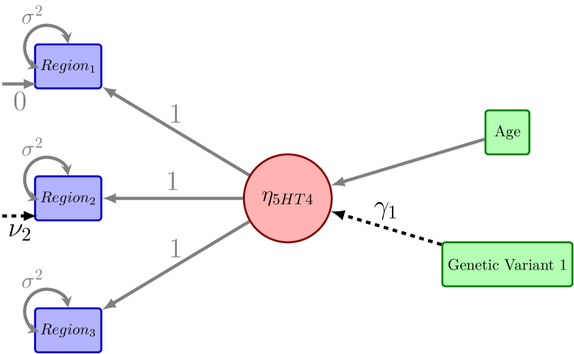
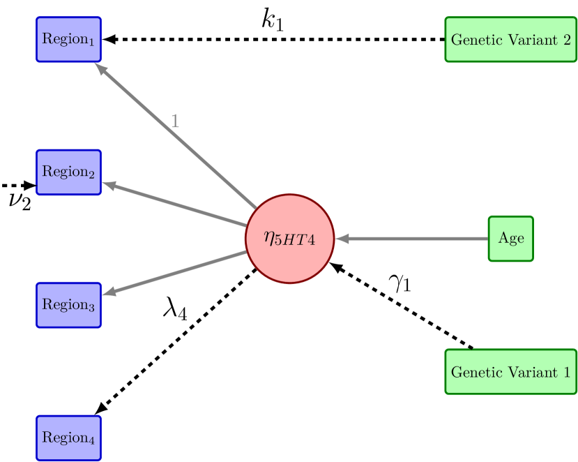
Study A : mixed model

Study B : single factor model

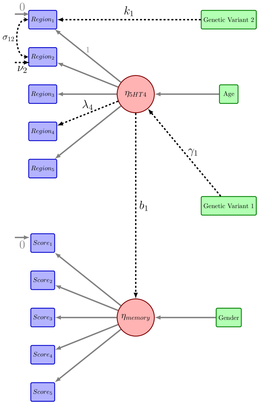
Study C : two latent variable model

Figure 3: Path diagram of the LVM associated with each simulation: endogenous variables are represented in blue, latent variables in red, and exogenous variables in green. The full arrows represent the generative model and symbols above these arrows represent constraints, e.g. in 3Study B the residual variances of $Y_{1}$, $Y_{2}$, $Y_{3}$ are constrained to have the same value. The values of the parameters in the generative model were 0 for the intercept and 1 for all the other parameters. The union of the full and dotted arrows represent the investigator models. Wald tests were performed for the parameters represented by a dotted arrow, e.g. $\nu_{2}$, $\gamma_{1}$ in 3Study B.

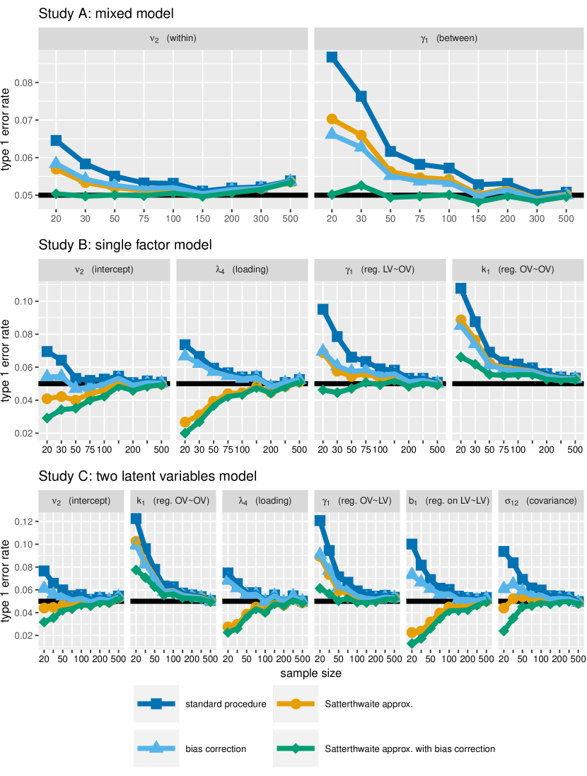
Figure 4: Type 1 error rate of the Wald test for study A, B and C at various sample sizes. The type 1 error rates for the parameters that are not shown on the graph (e.g., testing $\lambda_{2}=1$) are similar to the ones shown (e.g., testing $\lambda_{4}=0$). At a given sample size, 20000 simulations were performed, meaning that the type 1 error rate is expected to fluctuate between 0.047 and 0.053.

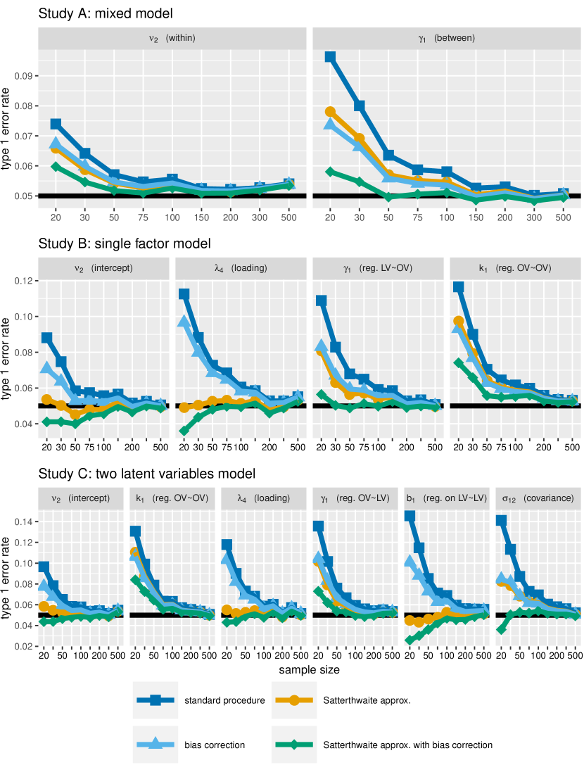
Figure 5: Type 1 error rate of the robust Wald test for study A, B and C at various sample sizes. The type 1 error rates for the parameters that are not shown on the graph (e.g., testing $\lambda_{2}=1$) are similar to the ones shown (e.g., testing $\lambda_{4}=0$). At a given sample size, 20000 simulations were performed, meaning that the type 1 error rate is expected to fluctuate between 0.047 and 0.053.

Wald test in a mixed model (Study A): the first LVM is equivalent to a random intercept model, where the endogenous variable is measured on three brain regions per subject. The resulting LVM has 7 parameters. The first null hypothesis tests whether the conditional expectation of the endogenous variable is the same between the first and second repetition (within subject parameter $\nu_{2}$). The second null hypothesis tests whether there is an effect of Genetic Variant 1 on all repetitions of the endogenous variable (between subject parameter $\gamma_{1}$).

The ML estimates of the variance parameters showed a small bias that was removed by our correction (table LABEL:SM-tab:biasMM in supplementary material LABEL:SM-SM:tableBiasML). Without correction, a moderate inflation of the type 1 error rate was observed for the Wald tests, e.g., $+0.015$ for $\nu_{2}$ and $+0.037$ for $\gamma_{1}$ when $n=20$ (first row of Figure 4). The bias correction combined with the Satterthwaite approximation provided a satisfactory control of the type 1 error rate, e.g., $0.050$ for $\nu_{2}$ and $\gamma_{1}$ when $n=20$.

Robust Wald test in a single factor model (Study B): Compared to the first simulation, the second LVM relaxes the assumption of common variance and covariance between the measurements, adds another polymorphism (Genetic Variant 2) and a fourth brain region. The resulting LVM had 15 parameters. Two additional null hypotheses are considered: whether the new region is correlated with the first one ($\lambda_{4}$) and whether there is an effect of Genetic Variant 2 on the first region ($k_{1}$).

The simulation indicates that the ML-estimator of the residual variance and of the variance of the latent variable were downward biased (table LABEL:SM-tab:biasFactor in supplementary material LABEL:SM-SM:tableBiasML), i.e. the estimated variance are too small. For instance, for $n$=20, the average bias was -0.125 for the residual variance and -0.150 for the variance of the latent variable (1 is the true value). The proposed correction was partially able to correct the bias, e.g. for $n$=20, the average bias became -0.029 for the residual variance and to -0.018 for the variance of the latent variable. Without correction, the inflation of the type 1 error rate in the robust Wald test was dependent on the coefficient (second row of Figure 5): $+0.038$ for $\nu_{2}$, $+0.063$ for $\lambda_{4}$, $+0.059$ for $\gamma_{1}$, and $+0.067$ for $k_{1}$ when $n=20$. The complete correction provided a satisfactory control for $\nu_{2}$ and $\gamma_{1}$ (type 1 error of $0.041$ and $0.056$, respectively for $n=20$) but was slightly too liberal for $k_{1}$ (type 1 error of $0.074$) and slightly too conservative for $\lambda_{4}$ (type 1 error of $0.036$).

Wald test in a LVM with two latent variables (Study C): we now add a new latent variable ($\eta_{memory}$) and an additional measurement per latent variable. The resulting LVM had 36 parameters. The new null hypotheses tests whether, conditional on the latent variable, there is a residual covariance between the first two regions ($\sigma_{12}$) and whether the first latent variable influences the second ($b_{1}$).

The results were similar to study B: the covariance parameter $\sigma_{12}$ did not show any bias, whereas the correction reduced the bias for the other parameters (table LABEL:SM-tab:biasLVM in supplementary material LABEL:SM-SM:tableBiasML). The inflation of the type 1 error was especially noticeable because the model involved more parameters (third row of Figure 4). The bias correction alone reduced the inflation of the type 1 error rate by $0.01$ to $0.03$. When combined with the Satterthwaite correction, the resulting procedure was satisfying for $\gamma_{1}$ (type 1 error of $0.061$ when $n=20$), conservative for $\nu_{2}$, $\lambda_{4}$, $b_{1}$, and $\sigma_{12}$ (type 1 error of respectively $0.032$, $0.023$, $0.013$, $0.024$ when $n=20$), but still liberal for $k_{1}$ (type 1 error of $0.078$ when $n=20$).

Distribution of the Wald statistic in small samples: the simulation results show that the proposed correction does not always control the type 1 error rate exactly at the nominal level. This may be due to the fact that the estimated Wald statistics are not $t$-distributed or that our estimators of the variance and degrees of freedom behave poorly in small samples. In supplementary material LABEL:SM-SM:validityStudent, we compare the distribution of the Wald statistic obtained after correction to the empirical one (obtained by simulation). We found that our estimators performed well in scenario A. However, in scenario B and C, the corrected variance was slightly biased downward and the Satterthwaite estimator of the degrees of freedom performed poorly for some parameters. The Student’s $t$-distribution appeared to be a good approximation of the empirical distribution except for two types of parameters ($b_{1}$, $\sigma_{12}$).

8 Application of the small sample correction to real data

We now re-run the Wald tests presented at the end of section 3 using the small sample correction developped in sections 4, 5, and 6. Table 1 gives an overview of the statistical tests performed with or without correction and the associated type 1 error (obtained by simulation).

		ML				ML with correction
Application	parameter	$\sigma$	$df$	p-value	type 1 error	$\sigma$	$df$	p-value	type 1 error
A	$k_{1},k_{2},k_{3}$		$\infty$	$1.76\text{\times}{10}^{-03}$	10.22%		49.1	$1.23\text{\times}{10}^{-02}$	4.49%
B	$\gamma_{2}$	0.026	$\infty$	$5.11\text{\times}{10}^{-03}$	7.41%	0.027	65.4	$9.03\text{\times}{10}^{-03}$	5.59%
	$k_{1}$	0.016	$\infty$	$7.23\text{\times}{10}^{-06}$	6.14%	0.017	67.5	$4.80\text{\times}{10}^{-05}$	4.78%
C	$b_{1}$	2.106	$\infty$	$5.45\text{\times}{10}^{-04}$	6.32%	2.143	13.5	$4.53\text{\times}{10}^{-03}$	2.02%
	$b_{2}$	2.355	$\infty$	$4.21\text{\times}{10}^{-03}$	8.50%	2.429	10.0	$1.96\text{\times}{10}^{-02}$	3.71%
	$b_{3}$	2.041	$\infty$	$7.20\text{\times}{10}^{-02}$	8.41%	2.130	7.7	$1.24\text{\times}{10}^{-01}$	3.42%

Table 1: Statistical inference without (column ML) and with (column ML with correction) the proposed correction in the three applications (A, B, and C) considered. The parameter $\sigma$ refers to the standard error associated with the estimated parameter and $df$ refers to the degrees of freedom of the Wald statistic. The type 1 error is computed by simulation under the null hypothesis.

Growth of guinea pigs (Application A): the correction we proposed in this article shares similarities with the KR correction: we attempt to correct the bias of the ML estimator when estimating the variance parameters and to use a Student’s $t$-distribution to model the distribution of the Wald statistic. The techniques used however differ, e.g., our bias-corrected ML estimator is not identical to the REML estimator. Nevertheless, the estimates of the residual variance and the variance of the random intercept obtained with our correction were similar to those obtained with REML (relative difference <1%, Table 2). They were 19% and 11% larger than their corresponding ML estimates. The corrected test statistic was 4.02 with a corresponding p-value of 0.0123. Although our method does not replicate the results obtained with the KR correction exactly, it gives estimates of the same order of magnitude. To further validate our correction, we performed the same simulation study as in the uncorrected case and found a type 1 error of 0.045 with the proposed correction.

	ML	ML with correction	REML
residual variance	0.148	0.177	0.176
variance random intercept	0.349	0.389	0.389
statistic	5.024	4.019	4.247
degrees of freedom	$\infty$	49.11	43.59
p-value	0.0018	0.0123	0.0102

Table 2: Comparison of the ML estimates, the proposed correction, and the REML estimates (using KR correction, Kenward and Roger, (1997)) in application A.

Serotonin 4 receptor binding and genetic polymorphisms (Application B): compared to the ML-estimates of the variances parameters, the corrected (non-robust) variance estimates were larger by 23.9% (neocortex), 4.5% (caudate), 4.0% (putamen), 3.8% (hippocampus), 3.8% (amygdala), and 10.9% (latent variable). When using cluster robust standard errors, the corrected p-values were 0.009 for the effect of the BDNF val66met (+76% compared to the original p-value) and $4.8\;10^{-5}$ for the effect of 5-HTTLPR (+564%). The same simulation study as in the uncorrected case gives, after correction, a type 1 error of 0.056 for the BDNF val66met effect and 0.048 for the 5-HTTLPR effect. Since the type 1 error estimated by simulations is close to the nominal level after correction and the corrected p-values are still below the critical level, this new analysis supports the conclusions of the original article.

Serotonin 4 receptor binding and verbal memory recall (Application C): the bias correction increased the estimates of the variance parameters by a factor ranging between 4.8% to 21.2% (endogenous variables) and 9.1% to 10.2% (latent variables). The corrected p-values were 0.0045 for $b_{1}$ (+731% compared to the original p-value), 0.02 for $b_{2}$ (+366%), and 0.12 for $b_{3}$ (+72%). The same simulation study as in the uncorrected case gives, after correction, a type 1 of 0.02 for $b_{1}$, 0.037 for $b_{2}$, and 0.034 for $b_{3}$ after correction. This new analysis supports the existence of an association between serotonin 4 receptor binding and recall of positive and neutral words ($b_{1}$ and $b_{2}$). The parameter $b_{3}$ did not reach significance before correction, where the testing procedure is liberal, so we should retain the null hypothesis for $b_{3}$.

In these applications, although the correction did not affect the conclusion of the statistical tests (when using a significance threshold of 0.05), the corrected p-values were better calibrated and therefore better reflected the strength of evidence against the null hypothesis.

9 Discussion

Concerns have been raised in the applied scientific literature about the lack of statistical power and the lack of reliability of studies involving small samples, e.g., see Button et al., (2013) and Bakker et al., (2012). Compared to $t$-tests or linear regressions, multivariate approaches such as LVMs can be used to increase the power of testing procedures. They also provide a common framework to test the hypotheses of the investigator and to assess modeling assumptions. Although exact tests can be performed on univariate models, only approximate tests are tractable with LVMs. Using simulation studies, we performed a detailed investigation of control of the type 1 error rate when using Wald tests in LVMs with small samples. The overall conclusion from these simulations was that the type 1 error rate is inflated in small samples. For a sample size of 20, the type 1 error rate varied between 0.06 to 0.12 for Wald test and between 0.07 and 0.14 for robust Wald test. The nominal level of 0.05 was reach when the sample size reached 100 to 200, depending on the type of model parameter.

We proposed two corrections to obtain a better control of the type 1 error rate: a correction for the bias of the ML-estimator of the variance parameters and the use of a Student’s $t$-distribution instead of a normal distribution to account for the uncertainty in the estimate of the variance of the model parameters. The proposed corrections have some desirable features: (1) when combined, they match the traditional corrections performed in univariate linear models, (2) they match the uncorrected ML inference in large samples, (3) they are fast to compute, require no user input, and can be applied to a large variety of models, and (4) the first correction reduced the bias of the variance estimates and improved the control of the type 1 error in all studies. Regarding (3), our implementation had a very reasonable run time: 75 ms to 475 ms in Study A, 200 ms to 900 ms in Study B, and 1.5s to 6s in Study C. It converged in very few iterations, except with very small samples and complex LVMs. One drawback of the proposed testing procedure is that it is not parametrisation-invariant, meaning that different identifiability constrains (e.g., setting to 1 a loading in the measurement model or the variance of the latent variable) may lead to different p-values. This is a well known issue when using Wald tests, and not a specificity of our corrections. Alternative test statistics (e.g. likelihood ratio test) should be considered if this property is required (Larsen et al.,, 2003).

A careful inspection of the simulation results showed that using a $t$-distribution to model the distribution of the Wald statistics was a good approximation for most parameters. We think that the inexact control of the type 1 error in small samples is mainly due to the poor performance of our estimator of the degrees of freedom. The estimation of the standard error could also be improved; indeed our bias-correction does not completely remove the bias from the estimator of the variance parameter. A better bias correction may be achieved using the formula of Cox and Snell, (1968) for the small sample bias of the ML estimator. It gives an estimate of the small sample bias up to $o_{p}(n^{-1})$ but involves complex calculations (third order derivative of the likelihood). The extension of the correction to robust standard errors could also be improved. Indeed the small sample correction has been derived assuming that the model was correctly specified (more precisely that $\mathbb{E}\left[{\boldsymbol{\xi}_{i}(\boldsymbol{\theta})}^{\intercal}\boldsymbol{\xi}_{i}(\boldsymbol{\theta})\right]=\Omega(\boldsymbol{\theta})$ and $\mathcal{I}(\boldsymbol{\theta})^{-1}=\Sigma_{\boldsymbol{\hat{\theta}}}$) and the current approximation for the degrees of freedom does not depend on the choice of the clusters $\mathcal{G}_{1},\ldots,\mathcal{G}_{G}$. The estimation of the degree of freedom will perform poorly when the clusters contain many observations. We investigated other approximations (e.g., Pan and Wall, (2002)) but did not obtain satisfying results. Finally, we note that the Satterthwaite correction was derived for the expected information matrix. In theory, a similar correction could be derived for the observed information matrix, but it would require more tedious derivations and complexify the software implementation. Nevertheless, this may be necessary in specific contexts, e.g., see Savalei, (2010) for a case where the expected information does not give consistent standard errors (missing data problems). In our software package implementing the proposed corrections, we provide a function called calibrateType1 that can be used to assess the type 1 error of the corrected and uncorrected Wald tests via simulations - under the assumption that the investigator model is correctly specified. We hope that this will help to detect inflations in the type 1 error rate and improve the reliability of studies involving small samples.

As pointed out by one reviewer, alternative estimation techniques such as instrumental variables (IV, Bollen, (1996)), generalized least squares (GLS), and weighted least squares (WLS, Yuan and Bentler, (1997)) could compare favorably to ML in small samples. Although a comprehensive comparison between these estimation techniques is beyond the scope of the present article, we performed an additional simulation to compare ML, IV, GLS, and WLS on Study B under a correctly specified model (see supplementary material LABEL:SM-SM:comparison). We found that GLS and IV showed an inflation of the type 1 error in small samples that is similar in magnitude to ML (uncorrected). WLS failed to estimate the model parameter for $n=20$ and $n=30$; it also had the worst control of the type 1 error. This poor behavior of WLS in small samples is consistent with the existing litterature (Olsson et al.,, 2000). Given the appealing properties of IV (Bollen et al.,, 2007), it would be of interest to propose a small sample correction for IV estimation.

10 Acknowledgement

B.O. was supported by the Lundbeck foundation (R231-2016-3236). This project has received funding from the European Union’s Horizon 2020 research and innovation programme under the Marie Sklodowska-Curie grant agreement No 746850.

References

References

- Bakker et al., (2012) Bakker, M., van Dijk, A., and Wicherts, J. M. (2012). The rules of the game called psychological science. Perspectives on Psychological Science, 7(6):543–554.
- Bentler and Yuan, (1999) Bentler, P. M. and Yuan, K.-H. (1999). Structural equation modeling with small samples: Test statistics. Multivariate behavioral research, 34(2):181–197.
- Bollen, (1996) Bollen, K. A. (1996). An alternative two stage least squares (2SLS) estimator for latent variable equations. Psychometrika, 61(1):109–121.
- Bollen et al., (2007) Bollen, K. A., Kirby, J. B., Curran, P. J., Paxton, P. M., and Chen, F. (2007). Latent variable models under misspecification: two-stage least squares (2SLS) and maximum likelihood (ML) estimators. Sociological Methods & Research, 36(1):48–86.
- Button et al., (2013) Button, K. S., Ioannidis, J. P., Mokrysz, C., Nosek, B. A., Flint, J., Robinson, E. S., and Munafò, M. R. (2013). Power failure: why small sample size undermines the reliability of neuroscience. Nature Reviews Neuroscience, 14(5):365.
- Carpenter and Bithell, (2000) Carpenter, J. and Bithell, J. (2000). Bootstrap confidence intervals: when, which, what? a practical guide for medical statisticians. Statistics in medicine, 19(9):1141–1164.
- Cox and Snell, (1968) Cox, D. R. and Snell, E. J. (1968). A general definition of residuals. Journal of the Royal Statistical Society. Series B (Methodological), pages 248–275.
- da Cunha-Bang et al., (2018) da Cunha-Bang, S., Fisher, P. M., Hjordt, L. V., Perfalk, E., Beliveau, V., Holst, K., and Knudsen, G. M. (2018). Men with high serotonin 1b receptor binding respond to provocations with heightened amygdala reactivity. NeuroImage, 166:79–85.
- Deen et al., (2017) Deen, M., Hansen, H. D., Hougaard, A., da Cunha-Bang, S., Nørgaard, M., Svarer, C., Keller, S. H., Thomsen, C., Ashina, M., and Knudsen, G. M. (2017). Low 5-ht1b receptor binding in the migraine brain: A pet study. Cephalalgia.
- Fisher et al., (2017) Fisher, P., Ozenne, B., Svarer, C., Adamsen, D., Lehel, S., Baaré, W., Jensen, P., and Knudsen, G. (2017). Bdnf val66met association with serotonin transporter binding in healthy humans. Translational psychiatry, 7(2):e1029.
- Fisher et al., (2015) Fisher, P. M., Holst, K. K., Adamsen, D., Klein, A. B., Frokjaer, V. G., Jensen, P. S., Svarer, C., Gillings, N., Baare, W. F., Mikkelsen, J. D., et al. (2015). Bdnf val66met and 5-httlpr polymorphisms predict a human in vivo marker for brain serotonin levels. Human brain mapping, 36(1):313–323.
- Harville, (1977) Harville, D. A. (1977). Maximum likelihood approaches to variance component estimation and to related problems. Journal of the American Statistical Association, 72(358):320–338.
- Herzog et al., (2007) Herzog, W., Boomsma, A., and Reinecke, S. (2007). The model-size effect on traditional and modified tests of covariance structures. Structural Equation Modeling, 14(3):361–390.
- Holst and Budtz-Jørgensen, (2013) Holst, K. K. and Budtz-Jørgensen, E. (2013). Linear latent variable models: the lava-package. Computational Statistics, 28(4):1385–1452.
- Jiang and Yuan, (2017) Jiang, G. and Yuan, K.-H. (2017). Four new corrected statistics for SEM with small samples and nonnormally distributed data. Structural Equation Modeling: A Multidisciplinary Journal, 24(4):479–494.
- Kauermann and Carroll, (2001) Kauermann, G. and Carroll, R. J. (2001). A note on the efficiency of sandwich covariance matrix estimation. Journal of the American Statistical Association, 96(456):1387–1396.
- Kenward and Roger, (1997) Kenward, M. G. and Roger, J. H. (1997). Small sample inference for fixed effects from restricted maximum likelihood. Biometrics, pages 983–997.
- Kuznetsova et al., (2017) Kuznetsova, A., Brockhoff, P. B., and Christensen, R. H. B. (2017). lmertest package: tests in linear mixed effects models. Journal of Statistical Software, 82(13).
- Larsen et al., (2003) Larsen, P. V., Jupp, P., et al. (2003). Parametrization-invariant wald tests. Bernoulli, 9(1):167–182.
- Maydeu-Olivares, (2017) Maydeu-Olivares, A. (2017). Maximum likelihood estimation of structural equation models for continuous data: Standard errors and goodness of fit. Structural Equation Modeling: A Multidisciplinary Journal, 24(3):383–394.
- McNeish, (2016) McNeish, D. (2016). On using bayesian methods to address small sample problems. Structural Equation Modeling: A Multidisciplinary Journal, 23(5):750–773.
- Muthén and Muthén, (2017) Muthén, L. K. and Muthén, B. O. (2017). Mplus user’s guide. eighth edition.
- Olsson et al., (2000) Olsson, U. H., Foss, T., Troye, S. V., and Howell, R. D. (2000). The performance of ML, GLS, and WLS estimation in structural equation modeling under conditions of misspecification and nonnormality. Structural equation modeling, 7(4):557–595.
- Pan and Wall, (2002) Pan, W. and Wall, M. M. (2002). Small-sample adjustments in using the sandwich variance estimator in generalized estimating equations. Statistics in medicine, 21(10):1429–1441.
- Parr, (1983) Parr, W. C. (1983). A note on the jackknife, the bootstrap and the delta method estimators of bias and variance. Biometrika, 70(3):719–722.
- Pek and Wu, (2015) Pek, J. and Wu, H. (2015). Profile likelihood-based confidence intervals and regions for structural equation models. Psychometrika, 80(4):1123–1145.
- Perfalk et al., (2017) Perfalk, E., da Cunha-Bang, S., Holst, K. K., Keller, S., Svarer, C., Knudsen, G. M., and Frokjaer, V. G. (2017). Testosterone levels in healthy men correlate negatively with serotonin 4 receptor binding. Psychoneuroendocrinology, 81:22–28.
- Rosseel, (2012) Rosseel, Y. (2012). lavaan: An R package for structural equation modeling. Journal of Statistical Software, 48(2):1–36.
- Satorra and Bentler, (1994) Satorra, A. and Bentler, P. M. (1994). Corrections to test statistics and standard errors in covariance structure analysis. Latent Varaibles Analysis: Applications to Developmental Research.
- Savalei, (2010) Savalei, V. (2010). Expected versus observed information in SEM with incomplete normal and nonnormal data. Psychological methods, 15(4):352.
- Stenbæk et al., (2017) Stenbæk, D. S., Fisher, P. M., Ozenne, B., Andersen, E., Hjordt, L. V., McMahon, B., Hasselbalch, S. G., Frokjaer, V. G., and Knudsen, G. M. (2017). Brain serotonin 4 receptor binding is inversely associated with verbal memory recall. Brain and behavior, 7(4).
- Wei et al., (1998) Wei, B.-C., Hu, Y.-Q., and Fung, W.-K. (1998). Generalized leverage and its applications. Scandinavian Journal of statistics, 25(1):25–37.
- White, (1982) White, H. (1982). Maximum likelihood estimation of misspecified models. Econometrica: Journal of the Econometric Society, pages 1–25.
- Wu and Lin, (2016) Wu, H. and Lin, J. (2016). A scaled f distribution as an approximation to the distribution of test statistics in covariance structure analysis. Structural Equation Modeling: A Multidisciplinary Journal, 23(3):409–421.
- Yuan and Bentler, (1997) Yuan, K.-H. and Bentler, P. M. (1997). Mean and covariance structure analysis: Theoretical and practical improvements. Journal of the American statistical association, 92(438):767–774.