Quaternion Hardy Functions for Local Images Feature Representation

Abstract

This paper is concerned with the applications of local features of the quaternion Hardy function. The feature information can be provided by the polar form of the quaternion Hardy function, such as the local attenuation and local phase vector. By using the generalized Cauchy-Riemann equations of local features, four various kinds of edge detectors are newly developed. The experiment results show that the amplitude-based edge detectors perform the envelope of test images while the phase-based edge detectors give the detail of the test images. Our proposed algorithms greatly outperform existing schemes.

Keywords: Quaternion; quaternion analytic signal; edge detection; Poisson operator.

AMS Mathematical Subject Classification: 44A15; 35F15; 70G10

1 Introduction

The edge detection is a preprocessing step in image analysis and computer vision. It aims to preserve the important structural properties in an image, hence, it is an crucial part in the computer vision-based applications. Such as color edge detection [1], motion [22], heart rate detection [2], and so on [27, 31]. There are a variety of edge detectors which have been devised [3]. The classical differentiation based edge detection identifies pixel locations with brightness changes by gradient operators, such as the Canny edge detection which is the popular choice for applications. The disadvantage of the differentiation based edge detection methods is the noise-sensitivity. In our paper, our approaches are based on the quaternion Hardy function, which is obtained by quaternion analytic signal being holomorphically extended into the upper (lower) half-space of two quaternion variables.

The analytic signal has lots of applications in signal and image processing [4, 18, 5]. The polar form of an analytic signal provides the signal features, such as the local amplitude and phase, which contain structural information of the signal, this fact enlightens us to apply them on image edge detection. By an original signal convoluting with the Poisson and conjugate Poisson integral, respectively, the analytic signal can be analytic continued into the upper (lower) Hardy space to be a Hardy function. Therefore Hardy function can handle various types of noises. Motivated by their excellent properties, high dimension extension was studied in several complex variable space [18, 19], quaternion space [16, 9, 6] and Clifford space [24, 28]. Generalizations under various transformations were analyzed, such as quaternion Fourier transform(QFT) [7, 6, 19] and quaternion linear canonical transform[23].

By convoluting Riesz kernel in higher dimensions, M.Felsberg and G.Sommer in 2001 [9] first studied the monogenic signal. Later, in 2004, they [16] proposed the monogenic scale-space, which is extension of the Hardy space in the higher dimension. The relationship between the local features of the monogenic scale function in the intrinsically 1D cases are deduced in [16], they satisfied the Cauchy-Riemann equations. In this paper, they also proposed a edge detection approach based on the phase of intrinsically 1D monogenic signals, it is called the differential phase congruency (DPC) method. While in the case of the function is not intrinsically 1D, the study was derived by Yan et al [28], The modified differential phase congruency (MDPC) was analyzed as the edge detector in their paper [28].

In [6],the quaternion analytic signal is one of the generalization of the analytic signal in high dimension. It corresponds to a boundary value of a quaternion Hardy function which is holomorphic in two quaternion variables $s_{1}=t_{1}+{\bf i}y_{1},s_{2}=t_{2}+{\bf j}y_{2}$. The quaternion Hardy function also provides the local features: the local attenuation, local phase and the local phase-vector. To the best of our knowledge, the relations between the features of quaternion Hardy function have not been carried out. In this paper, we will study the connection between them. The contributions of this paper are summarized as follows.

• By the generalized Cauchy-Riemann equations, the relations between the features of quaternion Hardy function are derived.

• The Phase-Based and Amplitude-based methods for edge detection filters are proposed. Theoretical and experiment results are established, respectively.

The remainder of the paper is organized as follows. Section 2 reviews some basic concepts. Section 3 gives the relationship of the features of quaternion Hardy function and proposes four novel edge detection approaches which are based on the features of quaternion Hardy function. Section 4 shows the experiment results. Section 5 gives the conclusion and future work.

2 Preliminaries

This section is devoted to the exposition of basic preliminary material which we use extensively throughout of this paper.

2.1 Quaternion Algebra

The notation $\mathbb{H}$ means the Hamiltonian skew field of quaternions, which can represent multidimensional signal as a holistic signal [10, 11, 12, 13, 14, 15]. A quaternion-value number takes a form

$$Q:=Q_{0}+{{\bf i}}Q_{1}+{{\bf j}}Q_{2}+{{\bf k}}Q_{3},$$ (1)

where $Q_{k}\in\mathbb{R},k=0,1,2,3,$ $\{1,{\bf i},{\bf j},{\bf k}\}$ is a quaternion orthogonal basis, and obeys the Hamilton’s multiplication rules:

$${\bf i}^{2}={\bf j}^{2}={\bf k}^{2}={\bf i}{\bf j}{\bf k}=-1.$$

Denote the various notations of quaternion-value number $Q$ as follows

• the Scalar part : ${\rm{Sc}}[Q]:=Q_{0}$,

• the ${\bf i}$ part : ${\rm{Vec}({\bf i})}[Q]:=Q_{1}$,

• the ${\bf j}$ part : ${\rm{Vec}({\bf j})}[Q]:=Q_{2}$,

• the ${\bf k}$ part : ${\rm{Vec}({\bf k})}[Q]:=Q_{3}$,

• the Vector part: $\underline{Q}$:=${\bf i}Q_{1}+{\bf j}Q_{2}+{\bf k}Q_{3}.$

$Q^{\ast}:=Q_{0}-{\bf i}Q_{1}-{\bf j}Q_{2}-{\bf k}Q_{3}.$ is denoted the conjugate of a quaternion $Q$. $|Q|:=\sqrt{QQ^{\ast}}=\sqrt{Q^{\ast}Q}=\sqrt{Q_{0}^{2}+Q_{1}^{2}+Q_{2}^{2}+Q_{3}^{2}}.$ is the modulus of $Q\in\mathbb{H}$. It is easy to verify that for $0\not=Q_{0}+\underline{Q}\in\mathbb{H}$, the inverse of $Q$ can be defined by

$$Q=(Q_{0}+\underline{Q})^{-1}:=\frac{\overline{Q_{0}+\underline{Q}}}{|QQ_{0}+\underline{Q}|^{2}}.$$

From Eq.$(\ref{u1})$, it follows that a quaternion-value function $f:\mathbb{R}^{2}\to\mathbb{H}$ can be expressed as

$$g(t_{1},t_{2})=g_{0}(t_{1},t_{2})+{\bf i}g_{1}(t_{1},t_{2})+{\bf j}g_{2}(t_{1},t_{2})+{\bf k}g_{3}(t_{1},t_{2}),$$

where $f_{n}\in\mathbb{R},n=0,1,2,3$. Let $L^{p}(\mathbb{R}^{2},\mathbb{H}),$ ( integers $p\geq$ 1) be the space of all quaternion-value function in $\mathbb{R}^{2},$ whose quaternion-value modules are defined by

$$L^{p}(\mathbb{R}^{2},\mathbb{H}):=\{g|g:\mathbb{R}^{2}\to\mathbb{H},\|g\|_{p}:=\left(\int_{\mathbb{R}^{2}}|g(t_{1},t_{2})|^{p}dt_{1}dt_{2}\right)^{\frac{1}{p}}<\infty\}.$$

There are different kinds of Quaternion Fourier transform (QFT) [8, 21]. In this paper, we derive the main results associated with the following QFT[8, 21] , which is defined by

$$\mathcal{F}[g](\omega_{1},\omega_{2}):=\int_{\mathbb{R}^{2}}e^{-{{\bf i}}\omega_{1}t_{1}}g(t_{1},t_{2})e^{{-{\bf j}}\omega_{2}t_{2}}dt_{1}dt_{2}.$$

where $g\in L^{1}(\mathbb{R}^{2},\mathbb{H}).$

2.2 Quaternion Hardy scale Space

There are various ways to analysis analytic signal to higher dimensional space [6, 29]. In this paper, the generalization is motivated by [6] using the quaternion analysis. Firstly, let’s recall definitions and properties of the quaternion partial and total Hilbert transforms associated with QFT [20, 23] .

Definition 2.1

[23] The quaternion partial Hilbert transform QPHT $\mathcal{H}_{1}$ and the quaternion total Hilbert transform QTHT $\mathcal{H}_{2}$ of $f$ are given by

$$\mathcal{H}_{1}[g(\cdot,t_{2})](t_{1}) := \frac{1}{\pi}p.v.\int_{\mathbb{R}}\frac{g(\tau,t_{2})}{t_{1}-\tau}d\tau,$$ (2)

$$\mathcal{H}_{1}[g(t_{1},\cdot)](t_{2}) := \frac{1}{\pi}p.v.\int_{\mathbb{R}}\frac{g(t_{1},\tau)}{t_{2}-\tau}d\tau,$$ (3)

$$\mathcal{H}_{2}[g(\cdot,\cdot)](t_{1},t_{2}) := \frac{1}{\pi^{2}}p.v.\int_{\mathbb{R}^{2}}\frac{g(\tau,\nu)}{(t_{1}-\tau)(t_{2}-\nu)}d\tau d\nu,$$ (4)

where $f$ is a generally quaternion-value function such that Eqs. $(\ref{deH1}),(\ref{deH2})$ and $(\ref{H3})$ are well defined.

Taking the QFT of Eqs. $(\ref{deH1}),(\ref{deH2})$ and $(\ref{H3})$ , we obtain that

$$\mathcal{F}[\mathcal{H}_{1}[g(\cdot,t_{2})](t_{1})](\omega_{1},\omega_{2}) = -\frac{1}{|\omega_{1}|}\mathcal{F}[\partial g/\partial t_{1}](\omega_{1},\omega_{2}).$$

$$\mathcal{F}[\mathcal{H}_{1}[g(t_{1},\cdot)](t_{2})](\omega_{1},\omega_{2}) = -\frac{1}{|\omega_{2}|}\mathcal{F}[\partial g/\partial t_{2}](\omega_{1},\omega_{2}).$$

$$\mathcal{F}[\mathcal{H}_{2}[g]](\omega_{1},\omega_{2}) = -\frac{1}{|\omega_{1}\omega_{2}|}\mathcal{F}[\partial^{2}g/\partial t_{1}\partial t_{2}](\omega_{1},\omega_{2}).$$

Hence, the QPHT $\mathcal{H}_{i}$ ($i=1,2$) and QTHT $\mathcal{H}_{2}$ have functions of the edge detectors [21].

The quaternion analytic signal [20] was defined by an original signal and its QPHT and QTHT as following.

Definition 2.2 (Quaternion Analytic Signal)

[20] The quaternion analytic signal $g_{q}$ of $g$ can be defined by

$$g_{q}(t_{1},t_{2}):=g(t_{1},t_{2})+{\bf i}\mathcal{H}_{1}[g(\cdot,t_{2})](t_{1})+\mathcal{H}_{1}[g(t_{1},\cdot)](t_{2}){\bf j}+{\bf i}\mathcal{H}_{2}[g](t_{1},t_{2}){\bf j},$$

where $g(t_{1},t_{2})$ is a quaternion-value function such that $g_{q}$ is well defined, that is, Eqs. $(\ref{deH1}),(\ref{deH2})$ and $(\ref{H3})$ are well defined.

Remark 2.1

When $f\in L^{2}(\mathbb{R}^{2},\mathbb{R}),$ then the definition is the same as in papers [7, 6].

Let $g\in L^{2}(\mathbb{R}^{2},\mathbb{H})$, we have

$$\mathcal{F}[g_{q}](\omega_{1},\omega_{2})=(1+sgn(\omega_{1}))(1+sgn(\omega_{2}))\mathcal{F}[g](\omega_{1},\omega_{2}).$$

Let us now study quaternion Hardy scales space, which is the Hardy space in quaternion algebra setting.

Definition 2.3

[20](Quaternion Hardy Scales Space $\mathbb{QS}(\mathbb{CS}_{{\bf i}{\bf j}}^{+},\mathbb{H})$) Quaternion Hardy scales Space $\mathbb{QS}(\mathbb{CS},\mathbb{H})$ is the class of quaternion Hardy functions (QHF) $g(s_{1},s_{2})$ which are defined on the upper half space $\mathbb{CS}$ and satisfies the following conditions:

1. $\frac{\partial}{\partial\overline{s_{1}}}g=0,$

2. $g\frac{\partial}{\partial\overline{s_{2}}}=0,$

3. $\int_{\mathbb{R}^{2}}|g(t_{1}+{\bf i}y_{1},tx_{2}+{\bf j}y_{2})|^{2}dt_{1}dt_{2}<C,$ for $y_{1}>0,y_{2}>0$,

where $\mathbb{CS}:=\{(s_{1},s_{2})|s_{1}:=t_{1}+{\bf i}y_{1},s_{2}:=t_{2}+{\bf j}y_{2},y_{1}>0,y_{2}>0\}.$

Due to the non-commutativity of the quaternions, the operators $\frac{\partial}{\partial\overline{s_{1}}}$ and$\frac{\partial}{\partial\overline{s_{2}}}$ are applied to quaternion-value function from the left and right,respectively. The parameters $y_{1}$ and $y_{2}$ are regarded as the scales.

Studying the Riemann-Hilbert problem in $\mathbb{CS},f\in L^{2}(\mathbb{R}^{2},\mathbb{H}),$

$$\frac{\partial}{\partial\overline{z_{1}}}g(s_{1},s_{2})=0,\quad(s_{1},s_{2})\in\mathbb{CS}.$$

$$g(s_{1},s_{2})\frac{\partial}{\partial\overline{s_{2}}}=0,\quad(s_{1},s_{2})\in\mathbb{CS}.$$

$$\mathcal{F}[g](\omega_{1},\omega_{2})=\left(1+sign(\omega_{1})\right)\left(1+sign(\omega_{2})\right)\mathcal{F}[h](\omega_{1},\omega_{2}),\quad(\omega_{1},\omega_{2})\in\mathbb{R}^{2},$$

The solutions are obtained by

$$g(s_{1},s_{2})=\frac{1}{2\pi{\bf i}}\int_{\mathbb{R}^{2}}\frac{4h(x,y)}{(x-s_{1})(y-s_{2})}dxdy\frac{1}{2\pi{\bf j}},$$ (5)

where $\frac{h(x,y)}{(x-s_{1})(y-s_{2})}=\frac{(\overline{(x-s_{1})}h(x,y)\overline{(y-s_{2}))})}{|x-s_{1}|^{2}|y-s_{2}|^{2}},$ and hence from the Plemelj-Sokhotzkis formulae for quaternion [20],

$$g(t_{1},t_{2})=h(t_{1},t_{2})+{\bf i}\mathcal{H}_{1}[h(\cdot,t_{2})](t_{1})+\mathcal{H}_{1}[h(t_{1},\cdot)](t_{2}){\bf j}+{\bf i}\mathcal{H}_{2}[h](t_{1},t_{2}){\bf j},$$

which tells us that the quaternion analytic signal $g$ corresponds to the boundary value of a quaternion Hardy function in $\mathbb{CS}.$

Theorem 2.1

[20] A quaternion-value signal $f_{q}\in L^{2}(\mathbb{R}^{2},\mathbb{H}),$ is a quaternion analytic signal of $f\in L^{2}(\mathbb{R}^{2},\mathbb{H})$ if and only if $f_{q}$ is boundary value of the quaternion Hardy function in $\mathbb{CS}.$ i.e.. There exits quaternion Hardy function (QHF) $f_{q}(s_{1},s_{2})\in\mathbb{Q}(\mathbb{CS},\mathbb{H}),$ such that

$$f_{q}(s_{1},s_{2})=\frac{1}{2\pi{\bf i}}\int_{\mathbb{R}^{2}}\frac{4f(x,y)}{(x-s_{1})(y-s_{2})}dsdt\frac{1}{2\pi{\bf j}}=r+{\bf i}m_{1}+m_{2}{\bf j}+{\bf i}m_{3}{\bf j},$$

and

$$f_{q}(t_{1},t_{2})=\lim_{y_{1}\rightarrow 0^{+},y_{2}\rightarrow 0^{+}}f_{q}(t_{1}+{\bf i}y_{1},t_{2}+{\bf j}y_{2}).$$ (6)

That is,

$$f(t_{1},t_{2})=\lim_{y_{1}\rightarrow 0^{+},y_{2}\rightarrow 0^{+}}r(t_{1}+{\bf i}y_{1};t_{2}+{\bf i}y_{2}),$$

$$\mathcal{H}_{1}[f(\cdot,t_{2})](t_{1})=\lim_{y_{1}\rightarrow 0^{+},y_{2}\rightarrow 0^{+}}m_{1}(t_{1}+{\bf i}y_{1};t_{2}+{\bf i}y_{2}),$$

$$\mathcal{H}_{1}[f(t_{1},\cdot)](t_{2})=\lim_{y_{1}\rightarrow 0^{+},y_{2}\rightarrow 0^{+}}m_{2}(t_{1}+{\bf i}y_{1};t_{2}+{\bf i}y_{2}),$$

$$\mathcal{H}_{2}[f](t_{1},t_{2})=\lim_{y_{1}\rightarrow 0^{+},y_{2}\rightarrow 0^{+}}m_{3}(t_{1}+{\bf i}y_{1};t_{2}+{\bf i}y_{2}),$$

where the functions $r$ and $m_{n},n=1,2,3$ are constructed by the Poisson $P_{y_{1}}(t_{1}):=\frac{y_{1}}{y_{1}^{2}+t_{1}^{2}}$and the conjugate Poisson $Q_{y_{1}}(t_{1}):=\frac{t_{1}}{y_{1}^{2}+t_{1}^{2}}$ integrals, respectively. $*$ denotes the 2D convolution operator of quaternion-value functions $f$ and $g$ in $\mathbb{R}^{2},$ i.e., $f*g(t_{1},t_{2})=\int_{\mathbb{R}^{2}}f(x,y)g(t_{1}-x,t_{2}-y)dxdy$. That is,

$$r(t_{1}+{\bf i}y_{1};t_{2}+{\bf i}y_{2}) = r*P_{y_{1}}(t_{1})P_{y_{2}}(t_{2})$$

$$= \frac{1}{\pi^{2}}\int_{\mathbb{R}^{2}}\frac{y_{1}y_{2}r(x,y)}{(y_{1}^{2}+(t_{1}-x)^{2})(y_{2}^{2}+(t_{2}-y)^{2})}dxdy$$

$$m_{1}(t_{1}+{\bf i}y_{1};t_{2}+{\bf i}y_{2}) = r*Q_{y_{1}}(t_{1})P_{y_{2}}(t_{2})$$

$$= \frac{1}{\pi^{2}}\int_{\mathbb{R}^{2}}\frac{x_{1}y_{2}r(x,y)}{(y_{1}^{2}+(t_{1}-x)^{2})(y_{2}^{2}+(t_{2}-y)^{2})}dxdy,$$

$$m_{2}(t_{1}+{\bf i}y_{1};t_{2}+{\bf i}y_{2}) = r*P_{y_{1}}(t_{1})Q_{y_{2}}(t_{2})$$

$$= \frac{1}{\pi^{2}}\int_{\mathbb{R}^{2}}\frac{y_{1}t_{2}r(x,y)}{(y_{1}^{2}+(t_{1}-x)^{2})(y_{2}^{2}+(t_{2}-y)^{2})}dxdy,$$

$$m_{3}(t_{1}+{\bf i}y_{1};t_{2}+{\bf i}y_{2}) = r*Q_{y_{1}}(t_{1})Q_{y_{2}}(t_{2})$$

$$= \frac{1}{\pi^{2}}\int_{\mathbb{R}^{2}}\frac{x_{1}x_{2}r(x,y)}{(y_{1}^{2}+(t_{1}-x)^{2})(y_{2}^{2}+(t_{2}-y)^{2})}dxdy.$$

2.3 Local Features

In this paper, we study the case under the quaternion sense, in which the quaternion analytic signal $g(t_{1},t_{2})$ is defined by a real signal $r\in L^{2}(\mathbb{R}^{2},\mathbb{R})$,

$$g(t_{1},t_{2})=r(t_{1},t_{2})+{\bf i}\mathcal{H}_{1}[r(\cdot,t_{2})](t_{1})+\mathcal{H}_{1}[r(t_{1},\cdot)](t_{2}){\bf j}+{\bf i}\mathcal{H}_{2}[r](t_{1},t_{2}){\bf j},$$

and by Theorem 2.1, its quaternion Hardy function is obtained as follows:

$$g(s_{1},s_{2})=r(s_{1},s_{2})+{\bf i}m_{1}(s_{1},s_{2})+m_{2}(s_{1},s_{2}){\bf j}+{\bf i}m_{3}(s_{1},s_{2}){\bf j}.$$

And find applications of the local features of quaternion Hardy function in image processing.

Definition 2.4

[Local Features][20] Suppose that quaternion Hardy function $g(s_{1},s_{2})=r(s_{1},s_{2})+\underline{m}(s_{1},s_{2})\in\mathbb{QS}(\mathbb{CS},\mathbb{H})$ has the polar representation

$$g(s_{1},s_{2}) = A(s_{1},s_{2})e^{\frac{\underline{m}(s_{1},s_{2})}{|\underline{m}(s_{1},s_{2})|}\theta}=e^{a(s_{1},s_{2})+\underline{p}(s_{1},s_{2})},$$

where

$$A(s_{1},s_{2}):=|f(s_{1},s_{2})|=\sqrt{r(s_{1},s_{2})^{2}+|\underline{m}(s_{1},s_{2})|^{2}}$$

is called the local amplitude, the energetic information of $r$ is contained in it.

$$a(s_{1},s_{2}):=\ln A(s_{1},s_{2})=\frac{1}{2}\ln(r^{2}(s_{1},s_{2})+|\underline{m}|^{2}(s_{1},s_{2}))$$ (8)

is called the local attenuation,

$$\theta(s_{1},s_{2}):=\arctan\left(\frac{|\underline{m}(s_{1},s_{2})|}{r(s_{1},s_{2})}\right)$$ (9)

is called the local phase, the value of which is is between $0$ and $\pi$. The structural information of $r(s_{1},s_{2})$ is included in it.

$$\underline{p}(s_{1},s_{2}):=\frac{\underline{m}(s_{1},s_{2})}{|\underline{m}(s_{1},s_{2})|}\theta(s_{1},s_{2}),$$ (10)

is called the local phase vector.

We are now ready to proceed the main results.

3 Phase-Based and Amplitude-based approaches

3.1 Theoretical Basis

Suppose a complex function $C(t_{1},t_{2})=r(t_{1},t_{2})+{\bf i}m(t_{1},t_{2})=e^{a(t_{1},t_{2})+{\bf i}\theta(t_{1},t_{2})}$ is holomorphic and no zero points in the complex space, then the local attenuation $a(t_{1},t_{2})=\frac{1}{2}\ln(r^{2}+m^{2})$ and the local phase $\theta(x_{1},x_{2})=\arctan\left(\frac{m}{r}\right)$ are satisfied the Cauchy-Riemann equations as following, we have

$$\frac{\partial a}{\partial t_{2}}+\frac{\partial\theta}{\partial t_{1}}=0,$$

$$\frac{\partial a}{\partial t_{1}}-\frac{\partial\theta}{\partial t_{2}}=0.$$

In fact, if $g(s_{1},s_{2})=r(s_{1},s_{2})+\underline{m}(s_{1},s_{2})=e^{a(s_{1},s_{2})+\underline{p}(s_{1},s_{2})}$ is holomorphic respective to $s_{1},s_{2}$ in the upper half space $\mathbb{CS}$, in general, $a(s_{1},s_{2})+\underline{p}(s_{1},s_{2})$ is not holomorphic.

Example 3.1

Let $E(s_{1},s_{2})={s_{1}^{\ast}s_{2}^{\ast}\over|s_{1}|^{2}|s_{2}|^{2}}$ be the Cauchy kernel in $\mathbb{H}\setminus\{0\}$, which is holomorphic in $\mathbb{H}\setminus\{0\}$. Then, by straightforward computations, we have

$$a(s_{1},s_{2})+\underline{p}(z_{1},z_{2})$$

$$= \ln(\sqrt{t^{2}_{1}+y^{2}_{1}})+\ln(\sqrt{t^{2}_{2}+y^{2}_{2}})+\frac{-{\bf i}t_{2}y_{1}-{\bf j}t_{1}y_{2}+{\bf k}y_{1}y_{2}}{|-{\bf i}t_{2}y_{1}-{\bf j}t_{1}y_{2}+{\bf k}y_{1}y_{2}|}$$

$$\arctan\left(\frac{|-{\bf i}t_{2}y_{1}-{\bf j}t_{1}y_{2}+{\bf k}y_{1}y_{2}|}{t_{1}t_{2}}\right).$$

Applying the generalized Cauchy-Riemann operators ${\partial\over\partial\overline{s_{1}}}$, ${\partial\over\partial\overline{s_{2}}}$ on it left side and right side, respectively, we obtain

$${\partial\over\partial\overline{s_{1}}}(a(s_{1},s_{2})+\underline{p}(s_{1},s_{2}))\neq 0.\quad(m(s_{1},s_{2})+\underline{p}(s_{1},s_{2})){\partial\over\partial\overline{s_{2}}}\neq 0.$$

Therefore, $(a(s_{1},s_{2})+\underline{p}(s_{1},s_{2}))$ is not quaternion holomorphic respective to $s_{1},s_{2}.$

Problem 3.1

What is relations of the local features of quaternion Hardy function in high dimensions ?

Corollary 3.1 gives the answers for Problem 3.1. Theorem 3.1 shows the more detail relations between four components of $f$ and its local attenuation $a$ in higher dimensional spaces. Before we give our main results, we first need some lemmas.

Remark 3.1

For convenience, let

$$\underline{p}:=\underline{p}(s_{1},s_{2}),\underline{m}:=\underline{m}(s_{1},s_{2}),\theta:=\theta(s_{1},s_{2}).a:=a(s_{1},s_{2}),r:=r(s_{1},s_{2}).$$

Lemma 3.1

Set $\underline{p}(s_{1},s_{2})=\frac{\underline{m}(s_{1},s_{2})}{|\underline{m}(s_{1},s_{2})|}\theta(s_{1},s_{2}),$ which is defined in Eq. (10), Then we obtain

$$\frac{\partial\underline{p}}{\partial t_{i}}=\left(\theta-\sin\theta\cos\theta\right)\frac{\partial\frac{\underline{m}}{|\underline{m}|}}{\partial t_{i}}+\frac{r\frac{\partial\underline{m}}{\partial t_{i}}-\underline{m}\frac{\partial r}{\partial t_{i}}}{r^{2}+|\underline{m}|^{2}}.$$ (11)

$$\frac{\partial\underline{p}}{\partial y_{i}}=\left(\theta-\sin\theta\cos\theta\right)\frac{\partial\frac{\underline{m}}{|\underline{m}|}}{\partial y_{i}}+\frac{r\frac{\partial\underline{m}}{\partial y_{i}}-\underline{m}\frac{\partial r}{\partial y_{i}}}{r^{2}+|\underline{m}|^{2}}.$$ (12)

• Proof: By Eq. (10), we obtain

  $$\frac{\partial\underline{p}}{\partial t_{i}} = \frac{\partial}{\partial t_{i}}(\frac{\underline{m}}{|\underline{m}|}\theta)=\frac{\partial\frac{\underline{m}}{|\underline{m}|}}{\partial t_{i}}\theta+\frac{\underline{m}}{|\underline{m}|}\frac{\partial}{\partial t_{i}}\theta.$$ (13)

  By straightforward computation, we have

  $$\frac{\underline{m}}{|\underline{m}|}\frac{\partial}{\partial t_{i}}(\arctan\left(\frac{|\underline{m}|}{r}\right))=\frac{r\frac{\partial\underline{m}}{\partial t_{i}}-\underline{m}\frac{\partial r}{\partial t_{i}}}{r^{2}+|\underline{m}|^{2}}-\frac{r|\underline{m}|}{r^{2}+|\underline{m}|^{2}}\frac{\partial\frac{\underline{m}}{|\underline{m}|}}{\partial t_{i}}.$$ (14)

  Combining Eq. (13) and Eq. (14), we obtain Eq. (11). Similarly, we have Eq. (12).

Lemma 3.2

Let $f(s_{1},s_{2})=r(s_{1},s_{2})+\underline{m}(s_{1},s_{2})=e^{a(s_{1},s_{2})+\underline{p}(s_{1},s_{2})}\in\mathbb{QS}(\mathbb{CS},\mathbb{H})$, where $a(s_{1},s_{2})$ and $\underline{p}(s_{1},s_{2})$ are defined by (8) and (10), respectively. If $f$ has no zeros in the half space $\mathbb{CS}$. Then we have

$$\left(\frac{\partial}{\partial t_{1}}e^{\underline{p}}\right)e^{-\underline{p}}=\frac{u\frac{\partial\underline{m}}{\partial t_{1}}-\underline{m}\frac{\partial r}{\partial t_{1}}}{r^{2}+|\underline{m}|^{2}}-\sin^{2}\theta\frac{\partial\frac{\underline{m}}{|\underline{m}|}}{\partial t_{1}}\frac{\underline{m}}{|\underline{m}|}.$$ (15)

$$\left(\frac{\partial}{\partial y_{1}}e^{\underline{p}}\right)e^{-\underline{p}}=\frac{r\frac{\partial\underline{m}}{\partial y_{1}}-\underline{m}\frac{\partial r}{\partial y_{1}}}{r^{2}+|\underline{m}|^{2}}-\sin^{2}\theta\frac{\partial\frac{\underline{m}}{|\underline{m}|}}{\partial y_{1}}\frac{\underline{m}}{|\underline{m}|}.$$ (16)

$$e^{-\underline{p}}\left(\frac{\partial}{\partial t_{2}}e^{\underline{p}}\right)=\frac{r\frac{\partial\underline{m}}{\partial t_{i}}-\underline{m}\frac{\partial r}{\partial t_{i}}}{r^{2}+|\underline{m}|^{2}}-\frac{\underline{m}}{|\underline{m}|}\sin^{2}\theta\frac{\partial\frac{\underline{m}}{|\underline{m}|}}{\partial t_{2}}.$$ (17)

$$e^{-\underline{p}}\left(\frac{\partial}{\partial y_{2}}e^{\underline{p}}\right)=\frac{r\frac{\partial\underline{m}}{\partial y_{2}}-\underline{m}\frac{\partial r}{\partial y_{2}}}{r^{2}+|\underline{m}|^{2}}-\frac{\underline{m}}{|\underline{m}|}\sin^{2}\theta\frac{\partial\frac{\underline{m}}{|\underline{m}|}}{\partial y_{2}}.$$ (18)

• Proof:

  Using the generalized Euler formula $e^{\underline{p}}=e^{\frac{\underline{m}}{|\underline{m}|}\theta}=\cos\theta+\frac{\underline{m}}{|\underline{m}|}\sin\theta$, we have

  $$\left(\frac{\partial}{\partial t_{1}}e^{\underline{p}}\right)e^{-\underline{p}}$$ (19)

  $$= \frac{\partial}{\partial t_{1}}\left(\cos\theta+\frac{\underline{m}}{|\underline{m}|}\sin\theta\right)\left(\cos\theta-\frac{\underline{m}}{|\underline{m}|}\sin\theta\right)$$

  $$= \left(-\sin\theta\frac{\partial\theta}{\partial t_{1}}+\frac{\partial\frac{\underline{m}}{|\underline{m}|}}{\partial t_{1}}\sin\theta+\frac{\underline{m}}{|\underline{m}|}\cos\theta\frac{\partial\theta}{\partial t_{1}}\right)\left(\cos\theta-\frac{\underline{m}}{|\underline{m}|}\sin\theta\right)$$

  $$= \frac{\underline{m}}{|\underline{m}|}\frac{\partial\theta}{\partial t_{1}}+\sin\theta\cos\theta\frac{\partial\frac{\underline{m}}{|\underline{m}|}}{\partial t_{1}}-\sin^{2}\theta\frac{\partial\frac{\underline{m}}{|\underline{m}|}}{\partial t_{1}}\frac{\underline{m}}{|\underline{m}|}.$$

  From (19), we know that $(\frac{\partial}{\partial t_{1}}e^{\underline{p}})e^{-\underline{p}}$ is decided by $\frac{\underline{m}}{|\underline{m}|}\frac{\partial\theta}{\partial t_{1}}+\sin\theta\cos\theta\frac{\partial\frac{\underline{m}}{|\underline{m}|}}{\partial t_{1}}-\sin^{2}\theta\frac{\partial\frac{\underline{m}}{|\underline{m}|}}{\partial t_{1}}\frac{\underline{m}}{|\underline{m}|}$. Since $\underline{p}=\frac{\underline{m}}{|\underline{m}|}\theta$, we have

  $$\frac{\partial\underline{p}}{\partial t_{1}}=\frac{\partial\theta}{\partial t_{1}}\frac{\underline{m}}{|\underline{m}|}+\theta\frac{\partial\frac{\underline{m}}{|\underline{m}|}}{\partial t_{1}}.$$ (20)

  From Eq.(11), therefore, we obtain Eq.(15). Similarly, we obtain (16),(17),(18).

The next theorem contains one of main results.

Theorem 3.1

Let $f(s_{1},s_{2})=r(s_{1},s_{2})+\underline{m}(s_{1},s_{2})=e^{a(s_{1},s_{2})+\underline{p}(s_{1},s_{2})}\in\mathbb{QS}(\mathbb{CS},\mathbb{H})$, where $a(s_{1},s_{2})$ and $\underline{p}(s_{1},s_{2})$ are defined by (8) and (10), respectively. If $f$ has no zeros in the upper half space $\mathbb{CS}$. Then we have

$$\frac{\partial a}{\partial t_{1}}-\bigg{\{}\frac{u\frac{\partial m_{1}}{\partial y_{1}}-m_{1}\frac{\partial r}{\partial y_{1}}}{r^{2}+|\underline{m}|^{2}}-\sin^{2}\theta\frac{\partial\frac{m_{2}}{|\underline{m}|}}{\partial y_{1}}\frac{m_{3}}{|\underline{m}|}+\sin^{2}\theta\frac{\partial\frac{m_{3}}{|\underline{m}|}}{\partial y_{1}}\frac{m_{2}}{|\underline{m}|}\bigg{\}}=0.$$ (21)

$$\frac{\partial a}{\partial y_{1}}+\bigg{\{}\frac{r\frac{\partial m_{1}}{\partial t_{1}}-m_{1}\frac{\partial r}{\partial t_{1}}}{r^{2}(s_{1},s_{2})+|\underline{m}(s_{1},s_{2})|^{2}}-\sin^{2}\theta\frac{\partial\frac{m_{2}}{|\underline{m}|}}{\partial t_{1}}\frac{m_{3}}{|\underline{m}|}+\sin^{2}\theta\frac{\partial\frac{m_{3}}{|\underline{m}|}}{\partial t_{1}}\frac{m_{2}}{|\underline{m}|}\bigg{\}}=0.$$ (22)

$${\rm Vec({\bf j})}[\frac{\partial(e^{\underline{p}})e^{-\underline{p}}}{\partial t_{1}}+{\bf i}\frac{\partial(e^{\underline{p}})e^{-\underline{p}}}{\partial y_{1}}]=0.$$

$${\rm Vec({\bf k})}[\frac{\partial(e^{\underline{p}})e^{-\underline{p}}}{\partial t_{1}}+{\bf i}\frac{\partial(e^{\underline{p}})e^{-\underline{p}}}{\partial y_{1}}]=0.$$

$$\frac{\partial a}{\partial t_{2}}-\bigg{\{}\frac{r\frac{\partial m_{2}}{\partial y_{2}}-m_{2}\frac{\partial r(s_{1},s_{2})}{\partial y_{2}}}{r^{2}+|\underline{m}|^{2}}-\sin^{2}\theta\frac{\partial\frac{m_{1}}{|\underline{m}|}}{\partial y_{2}}\frac{m_{3}}{|\underline{m}|}+\sin^{2}\theta\frac{\partial\frac{m_{3}}{|\underline{m}|}}{\partial y_{2}}\frac{m_{1}}{|\underline{m}|}\bigg{\}}=0.$$ (23)

$$\frac{\partial a}{\partial y_{2}}+\bigg{\{}\frac{r\frac{\partial m_{2}}{\partial t_{2}}-m_{2}\frac{\partial r}{\partial t_{2}}}{r^{2}+|\underline{m}|^{2}}-\sin^{2}\theta\frac{\partial\frac{m_{1}}{|\underline{m}|}}{\partial t_{2}}\frac{m_{3}}{|\underline{m}|}+\sin^{2}\theta\frac{\partial\frac{m_{3}}{|\underline{m}|}}{\partial t_{2}}\frac{m_{1}}{|\underline{m}|}\bigg{\}}=0=0,$$ (24)

$${\rm Vec({\bf i})}[\frac{e^{-\underline{p}}\partial(e^{\underline{p}})}{\partial t_{2}}+\frac{e^{-\underline{p}}\partial(e^{\underline{p}})}{\partial y_{2}}{\bf j}]=0.$$ (25)

$${\rm Vec({\bf k})}[\frac{e^{-\underline{p}}\partial(e^{\underline{p}})}{\partial t_{2}}+\frac{e^{-\underline{p}}\partial(e^{\underline{p}})}{\partial y_{2}}{\bf j}]=0.$$ (26)

• Proof of Theorem 3.1: Since $f(s_{1},s_{2})=e^{m+\underline{p}}\in\mathbb{QS}(\mathbb{C}_{{\bf i}{\bf j}}^{+}))$, we have

  $$\left(\frac{\partial}{\partial t_{1}}+{\bf i}\frac{\partial}{\partial y_{1}}\right)e^{a+\underline{p}}=0.$$

  By straightforward computation, we have

  $$e^{a}\frac{\partial a}{\partial t_{1}}e^{\underline{p}}+e^{a}\frac{\partial e^{\underline{p}}}{\partial t_{1}}+e^{a}[{\bf i}\frac{\partial a}{\partial y_{1}}]e^{\underline{p}}+e^{a}({\bf i}\frac{\partial e^{\underline{p}}}{\partial y_{1}})=0.$$

  That is

  $$\frac{\partial a}{\partial t_{1}}+\frac{\partial e^{\underline{p}}}{\partial t_{1}}e^{-\underline{p}}+{\bf i}\frac{\partial a}{\partial y_{1}}+({\bf i}\frac{\partial e^{\underline{p}}}{\partial y_{1}})e^{-\underline{p}}=0.$$ (27)

  Therefore, the scale part of (27) is zero, and $\partial\frac{\left(\frac{\underline{m}}{|m|}\right)^{2}}{\partial t_{1}}=0,$ we have

  $${\rm Sc}\left[\frac{\partial a}{\partial t_{1}}+\frac{\partial e^{\underline{p}}}{\partial t_{1}}e^{-\underline{p}}+{\bf i}\frac{\partial m}{\partial y_{1}}+({\bf i}\frac{\partial e^{\underline{p}}}{\partial y_{1}})e^{-\underline{p}}\right]$$ (28)

  $$= \frac{\partial a}{\partial t_{1}}+{\rm Sc}[({\bf i}\frac{\partial e^{\underline{p}}}{\partial y_{1}})e^{-\underline{p}}]=0$$

  Moreover, from (15),

  $${\rm Sc}\bigg{[}\bigg{(}{\bf i}\frac{\partial(e^{\underline{p}})e^{-\underline{p}}}{\partial y_{1}}\bigg{)}\bigg{]}=-\bigg{\{}\frac{r\frac{\partial m_{1}}{\partial y_{1}}-m_{1}\frac{\partial r}{\partial y_{1}}}{r^{2}+|\underline{m}|^{2}}-\sin^{2}\theta\frac{\partial\frac{m_{2}}{|\underline{m}|}}{\partial y_{1}}\frac{m_{3}}{|\underline{m}|}+\sin^{2}\theta\frac{\partial\frac{m_{3}}{|\underline{m}|}}{\partial y_{1}}\frac{m_{2}}{|\underline{m}|}\bigg{\}}.$$

  we get the desired result (21).

  The three vector parts of Eq. (27) are all zero. Using Lemma 3.2 we find that

  $${\rm Vec({\bf i})}\left[\frac{\partial a}{\partial t_{1}}+\frac{\partial e^{\underline{p}}}{\partial t_{1}}e^{-\underline{p}}+{\bf i}\frac{\partial a}{\partial y_{1}}+({\bf i}\frac{\partial e^{\underline{p}}}{\partial y_{1}})e^{-\underline{p}}\right]$$ (29)

  $$= {\rm Vec({\bf i})}\left[\frac{\partial e^{\underline{p}}}{\partial t_{1}}e^{-\underline{p}}+{\bf i}\frac{\partial a}{\partial y_{1}}\right]$$

  $$= \frac{\partial a}{\partial y_{1}}+{\rm Sc}\left[(-{\bf i})\frac{\partial e^{\underline{p}}}{\partial t_{1}}e^{-\underline{p}}\right]=0.$$

  from (16), we obtain Eq.(22).

  $${\rm Vec({\bf j})}\left[\frac{\partial a}{\partial t_{1}}+\frac{\partial e^{\underline{p}}}{\partial t_{1}}e^{-\underline{p}}+{\bf i}\frac{\partial a}{\partial y_{1}}+({\bf i}\frac{\partial e^{\underline{p}}}{\partial y_{1}})e^{-\underline{p}}\right]$$

  $$= {\rm Vec({\bf j})}\left[\frac{\partial e^{\underline{p}}}{\partial t_{1}}e^{-\underline{p}}+({\bf i}\frac{\partial e^{\underline{p}}}{\partial y_{1}})e^{-\underline{p}}\right]=0.$$

  $${\rm Vec({\bf k})}\left[\frac{\partial a}{\partial t_{1}}+\frac{\partial e^{\underline{p}}}{\partial t_{1}}e^{-\underline{p}}+{\bf i}\frac{\partial a}{\partial y_{1}}+({\bf i}\frac{\partial e^{\underline{p}}}{\partial y_{1}})e^{-\underline{p}}\right]$$

  $$= {\rm Vec({\bf k})}\left[\frac{\partial e^{\underline{p}}}{\partial t_{1}}e^{-\underline{p}}+({\bf i}\frac{\partial e^{\underline{p}}}{\partial y_{1}})e^{-\underline{p}}\right]=0.$$

  Since

  $$e^{a+\underline{p}}\left(\frac{\partial}{\partial t_{2}}+{\bf j}\frac{\partial}{\partial y_{2}}\right)=0.$$

  Using the similar steps as in above, we have

  $$\frac{\partial a}{\partial t_{2}}+{\rm Sc}\left[e^{-\underline{p}}(\frac{\partial e^{\underline{p}}}{\partial y_{2}}){\bf j}\right]=0$$ (30)

  $$\frac{\partial a}{\partial y_{2}}-{\rm Sc}\left[e^{-\underline{p}}(\frac{\partial e^{\underline{p}}}{\partial t_{2}}){\bf j}\right]=0$$ (31)

  $${\rm Vec({\bf i})}\left[(e^{-\underline{p}}\frac{\partial e^{\underline{p}}}{\partial t_{2}})+e^{-\underline{p}}(\frac{\partial e^{\underline{p}}}{\partial y_{2}}){\bf j}\right]=0$$

  $${\rm Vec({\bf k})}\left[e^{-\underline{p}}(\frac{\partial e^{\underline{p}}}{\partial t_{2}})+e^{-\underline{p}}(\frac{\partial e^{\underline{p}}}{\partial y_{2}}){\bf j}\right]=0$$

  Using Lemma 3.2 and Eqs.(17), (18), we obtain Eqs.(23),(24),(25),(26).This completes the proof.

From Theorem 3.1, combing the Eqs.(28), (29), (30), (31), (19), (20), we have the following corollary, which show the relations of the local features of quaternion Hardy function.

Corollary 3.1

Let $f(s_{1},s_{2})=r(s_{1},s_{2})+\underline{m}(s_{1},s_{2})=e^{a(s_{1},s_{2})+\underline{p}(s_{1},s_{2})}\in\mathbb{QS}(\mathbb{C},\mathbb{H})$, If $f$ has no zeros in the upper half space $\mathbb{CS}$. Then we have

$$\frac{\partial a}{\partial t_{1}}+{\rm Vec({\bf i})}\left[\frac{\partial\underline{p}}{\partial y_{1}}-\theta\frac{\partial\frac{\underline{m}}{|\underline{m}|}}{\partial y_{1}}+\sin\theta\cos\theta\frac{\partial\frac{\underline{m}}{|\underline{m}|}}{\partial y_{1}}-\sin^{2}\theta\frac{\partial\frac{\underline{m}}{|\underline{m}|}}{\partial y_{1}}\frac{\underline{m}}{|\underline{m}|}\right]=0$$ (32)

$$\frac{\partial a}{\partial t_{2}}+{\rm Vec({\bf j})}\left[\frac{\partial\underline{p}}{\partial y_{2}}-\theta\frac{\partial\frac{\underline{m}}{|\underline{m}|}}{\partial y_{2}}+\sin\theta\cos\theta\frac{\partial\frac{\underline{m}}{|\underline{m}|}}{\partial y_{2}}-\frac{\underline{m}}{|\underline{m}|}\sin^{2}\theta\frac{\partial\frac{\underline{m}}{|\underline{m}|}}{\partial y_{2}}\right]=0$$ (33)

$$\frac{\partial a}{\partial y_{1}}-{\rm Vec({\bf i})}\left[\frac{\partial\underline{p}}{\partial t_{1}}-\theta\frac{\partial\frac{\underline{m}}{|\underline{m}|}}{\partial t_{1}}+\sin\theta\cos\theta\frac{\partial\frac{\underline{m}}{|\underline{m}|}}{\partial t_{1}}-\sin^{2}\theta\frac{\partial\frac{\underline{m}}{|\underline{m}|}}{\partial t_{1}}\frac{\underline{m}}{|\underline{m}|}\right]=0$$ (34)

$$\frac{\partial a}{\partial y_{2}}-{\rm Vec({\bf j})}\left[\frac{\partial\underline{p}}{\partial t_{2}}-\theta\frac{\partial\frac{\underline{m}}{|\underline{m}|}}{\partial t_{2}}+\sin\theta\cos\theta\frac{\partial\frac{\underline{m}}{|\underline{m}|}}{\partial t_{2}}-\frac{\underline{m}}{|\underline{m}|}\sin^{2}\theta\frac{\partial\frac{\underline{m}}{|\underline{m}|}}{\partial t_{2}}\right]=0$$ (35)

From this corollary, we also notice that

• Eqs. 32 and 33 show that the partial derivatives of the local attenuation $\frac{\partial a}{\partial t_{1}}$ and $\frac{\partial a}{\partial t_{2}}$ do not equal the the minus of the scale derivatives of the local phase-vector ${\partial\underline{p}\over\partial y_{1}}$ and ${\partial\underline{p}\over\partial y_{2}}$.

• Eqs. 34 and 35 show that the partial derivative of the local phase-vector ${\partial\underline{p}\over\partial t_{1}}$ and ${\partial\underline{p}\over\partial t_{2}}$ can not be given by the scale partial derivatives of the local attenuation $\frac{\partial a}{\partial y_{1}}$ and $\frac{\partial a}{\partial y_{2}}.$

3.2 Concrete Approaches

Let’s first introduce the Quaternion Differential Local Attenuation (QDLA) approach, which is based on the partial differentiation of the local attenuation in the $t_{1}$ and $t_{2}$ variables.

Method 3.1 (QDLA)

For $f=r+{\bf i}m_{1}+{\bf j}m_{2}+{\bf k}m_{3}\in\mathbb{QS}(\mathbb{CS},\mathbb{H})$ has no zeros in the half space $\mathbb{CS}$, the Quaternion Differential Local Attenuation (QDLA) approach has the formula

$$\frac{\partial a}{\partial t_{1}} = \frac{u\frac{\partial r}{\partial t_{1}}+|\underline{m}|\frac{\partial|\underline{m}|}{\partial t_{1}}}{r^{2}+|\underline{m}|^{2}}.$$

$$\frac{\partial a}{\partial t_{2}} = \frac{r\frac{\partial r}{\partial t_{2}}+|\underline{m}|\frac{\partial|\underline{m}|}{\partial t_{2}}}{r^{2}+|\underline{m}|^{2}}.$$

From Eqs. (21) and (23), the local maxima of the local amplitude is equivalent to Eqs. (Step 3.) and (Step 3.) for QHF, then we propose the next approach, named Modified Quaternion Differential Local Attenuation (MQDLA), which based on the local phase.

Method 3.2 (MQDLA)

For $f=r+{\bf i}m_{1}+{\bf j}m_{2}+{\bf k}m_{3}\in\mathbb{QS}(\mathbb{CS},\mathbb{H})$ has no zeros in the half space $\mathbb{CS}$, the MQDLA approach has the formula

$$p1=\frac{r\frac{\partial m_{1}}{\partial y_{1}}-m_{1}\frac{\partial r}{\partial y_{1}}}{r^{2}+|\underline{m}|^{2}}-\sin^{2}\theta\frac{\partial\frac{m_{2}}{|\underline{m}|}}{\partial y_{1}}\frac{m_{3}}{|\underline{m}|}+\sin^{2}\theta\frac{\partial\frac{m_{3}}{|\underline{m}|}}{\partial y_{1}}\frac{m_{2}}{|\underline{m}|}.$$ (36)

$$p2=\frac{r\frac{\partial m_{2}}{\partial y_{2}}-m_{2}\frac{\partial r}{\partial y_{2}}}{r^{2}+|\underline{m}(s_{1},s_{2})|^{2}}-\sin^{2}\theta\frac{\partial\frac{m_{1}}{|\underline{m}|}}{\partial y_{2}}\frac{m_{3}}{|\underline{m}|}+\sin^{2}\theta\frac{\partial\frac{m_{3}}{|\underline{m}|}}{\partial y_{2}}\frac{m_{1}}{|\underline{m}|}.$$ (37)

Then local attenuation has four variables, let us derivative the local attenuation with respect to the scales $y_{1},y_{2}$ to get the Scale Derivative Local Amplitude (SDLA) approach, which bases on the local amplitude.

Method 3.3 (SDLA)

For $f=r+{\bf i}m_{1}+{\bf j}m_{2}+{\bf k}m_{3}\in\mathbb{QS}(\mathbb{CS},\mathbb{H})$ has no zeros in the half space $\mathbb{CS}$, the SDLA approach has the formula

$$\frac{\partial a}{\partial y_{1}} = \frac{u\frac{\partial r}{\partial y_{1}}+|\underline{m}|\frac{\partial|\underline{m}|}{\partial y_{1}}}{r^{2}+|\underline{m}|^{2}}.$$

$$\frac{\partial a}{\partial y_{2}} = \frac{r\frac{\partial r}{\partial y_{2}}+|\underline{m}|\frac{\partial|\underline{m}|}{\partial y_{2}}}{r^{2}+|\underline{m}|^{2}}.$$

From Eqs. (22) and (24), the scale partial derivatives of the local attenuation$\frac{\partial a}{\partial y_{1}}$ and $\frac{\partial a}{\partial y_{2}}$ are equivalent to Eqs. (Step 3.) and (Step 3.) for QHF, respectively, then we propose the next approach, named Modified Scale Derivative Local Amplitude (MDSLA) approach, which bases on the local phase.

Method 3.4 (MSDLA)

For $f=r+{\bf i}m_{1}+{\bf j}m_{2}+{\bf k}m_{3}\in\mathbb{QS}(\mathbb{CS},\mathbb{H})$ has no zeros in the half space $\mathbb{CS}$, , the MSDLA approach has the formula

$$M1:=\frac{-r\frac{\partial m_{1}}{\partial t_{1}}+m_{1}\frac{\partial r}{\partial t_{2}}}{r^{2}+|\underline{m}|^{2}}+\sin^{2}\theta\frac{\partial\frac{m_{2}}{|\underline{m}|}}{\partial t_{1}}\frac{m_{3}}{|\underline{m}|}-\sin^{2}\theta\frac{\partial\frac{m_{3}}{|\underline{m}|}}{\partial t_{1}}\frac{m_{2}}{|\underline{m}|}$$ (38)

$$M2:=\frac{-r\frac{\partial m_{2}}{\partial t_{2}}+m_{2}\frac{\partial r}{\partial t_{2}}}{r^{2}+|\underline{m}|^{2}}+\sin^{2}\theta\frac{\partial\frac{m_{1}}{|\underline{m}|}}{\partial t_{2}}\frac{m_{3}}{|\underline{m}|}-\sin^{2}\theta\frac{\partial\frac{m_{3}}{|\underline{m}|}}{\partial t_{2}}\frac{m_{1}}{|\underline{m}|}$$ (39)

4 Experiments

In this section, In order to have an idea of the performance, the new approaches are not only compared to edge detection algorithms taken from the image processing toolbox of Matlab: Canny and Sobel edge detectors, but also compared ours to the phase congruency edge detectors, DPC [16] and MDPC [28]. The Comparative results of the proposed approaches $($ QDLA, MQDLA, SDLA, MSDLA $)$ and the Canny , Sobel, DPC, MDPC approachs are visualized in Fig. 3.

The approach of MDPC and DPC is used the Non-maximum suppress [25] to get thinner edge boundary,the radius is chosen r=1.5, for the MDPC, the lower and upper thresholds are 1.0 and 3.5, respectively. While for the DPC, the lower and upper thresholds are 2.0 and 3.5, respectively. And all parameters of Canny and Sobel are automatically generated by the Matlab algorithms in order to obtain a comparison of fully automatic approaches.

4.1 Algorithms

The flow of the image edge detection is shown in Figure 1 .

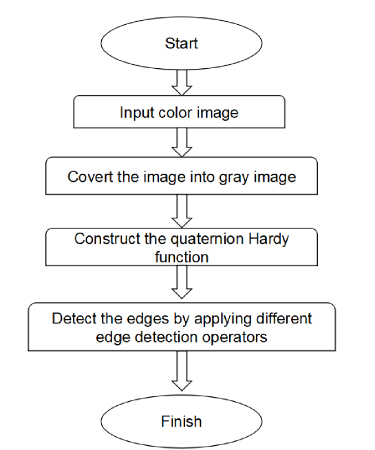
Figure 1: Flow chart for image edge detection.

Step 1.

Input image $r(t_{1},t_{2})$.

Step 2.

Poisson filtering : $r(t_{1}+{\bf i}y_{1},t_{2}+{\bf j}y_{2})=r*P_{y_{1}}(t_{1})P_{y_{2}}(t_{2})$ and and $m_{1}(t_{1}+{\bf i}y_{1},t_{2}+{\bf j}y_{2})=r*Q_{y_{1}}(x_{1})P_{y_{2}}(t_{2}),$ $m_{2}(t_{1}+{\bf i}y_{1},t_{2}+{\bf j}y_{2})=r*P_{y_{1}}(x_{1})Q_{y_{2}}(t_{2}),$ $m_{3}(t_{1}+{\bf i}y_{1},t_{2}+{\bf j}y_{2})=r*Q_{y_{1}}(x_{1})Q_{y_{2}}(t_{2}),$ for fixed scales $y_{1}=0.3,y_{1}=0.3$. From this step, we obtain the quaternion Hardy function

$$r_{q}(s_{1},s_{2})=r(s_{1},s_{2})+{\bf i}m_{1}(s_{1},s_{2})+m_{2}(s_{1},s_{2}){\bf j}+{\bf i}m_{3}(s_{1},s_{2}){\bf j}.$$

Step 3.

Select one of the algorithms to evaluate to obtain the gradient maps of these approach.:

QDLA approach

$$\frac{\partial a}{\partial t_{1}} = \frac{r\frac{\partial r}{\partial t_{1}}+|\underline{m}|\frac{\partial|\underline{m}|}{\partial t_{1}}}{r^{2}+|\underline{m}|^{2}}.$$

$$\frac{\partial a}{\partial t_{2}} = \frac{r\frac{\partial r}{\partial t_{2}}+|\underline{m}|\frac{\partial|\underline{m}|}{\partial t_{2}}}{r^{2}+|\underline{m}|^{2}}.$$

MQDLA approach

$$p1=\frac{r\frac{\partial m_{1}}{\partial y_{1}}-m_{1}\frac{\partial u}{\partial y_{1}}}{r^{2}+|\underline{m}|^{2}}-\sin^{2}\theta\frac{\partial\frac{m_{2}}{|\underline{m}|}}{\partial y_{1}}\frac{m_{3}}{|\underline{m}|}+\sin^{2}\theta\frac{\partial\frac{m_{3}}{|\underline{m}|}}{\partial y_{1}}\frac{m_{2}}{|\underline{m}|}.$$

$$p2=\frac{r\frac{\partial m_{2}}{\partial y_{2}}-m_{2}\frac{\partial r}{\partial y_{2}}}{r^{2}+|\underline{m}|^{2}}-\sin^{2}\theta\frac{\partial\frac{m_{1}}{|\underline{m}|}}{\partial y_{2}}\frac{m_{3}}{|\underline{m}|}+\sin^{2}\theta\frac{\partial\frac{m_{3}}{|\underline{m}|}}{\partial y_{2}}\frac{m_{1}}{|\underline{m}|}.$$

SDLA approach

$$\frac{\partial a}{\partial y_{1}} = \frac{r\frac{\partial r}{\partial y_{1}}+|\underline{m}|\frac{\partial|\underline{m}|}{\partial y_{1}}}{r^{2}+|\underline{m}|^{2}}.$$

$$\frac{\partial a}{\partial y_{2}} = \frac{r\frac{\partial r}{\partial y_{2}}+|\underline{m}|\frac{\partial|\underline{m}|}{\partial y_{2}}}{r^{2}+|\underline{m}|^{2}}.$$

MSDLA approach

$$M1:=\frac{-r\frac{\partial m_{1}}{\partial t_{1}}+m_{1}\frac{\partial r}{\partial t_{2}}}{r^{2}+|\underline{m}|^{2}}+\sin^{2}\theta\frac{\partial\frac{m_{2}}{|\underline{m}|}}{\partial t_{1}}\frac{m_{3}}{|\underline{m}|}-\sin^{2}\theta\frac{\partial\frac{m_{3}}{|\underline{m}|}}{\partial t_{1}}\frac{m_{2}}{|\underline{m}|}$$

$$M2:=\frac{-r\frac{\partial m_{2}}{\partial t_{2}}+m_{2}\frac{\partial r}{\partial t_{2}}}{r^{2}+|\underline{m}|^{2}}+\sin^{2}\theta\frac{\partial\frac{m_{1}}{|\underline{m}|}}{\partial t_{2}}\frac{m_{3}}{|\underline{m}|}-\sin^{2}\theta\frac{\partial\frac{m_{3}}{|\underline{m}|}}{\partial t_{2}}\frac{m_{1}}{|\underline{m}|}$$

Step 4.

For test images in Fig.2 , the non-maximum suppress is applied to these gradient maps such that the edges become thinner, the radius r=1.5 is chosen. For MSDLA detector, the lower and upper threshold values are 15 and 27, respectively. For the other approaches, the lower and upper threshold values are 3.8 and 5.5, respectively.

4.2 Experiment results

4.2.1 Visual comparisons

1. There are four original test images, namely fish, building, lane and liver (Figure 2), are applied for various edge detectors. The experiment results of various approaches with the fixed scales $y_{1}=0.3$ and $y_{2}=0.3$ are shown in Figure 3 . Some conclusions are reasonably drawn from these results (Figure 3).

   

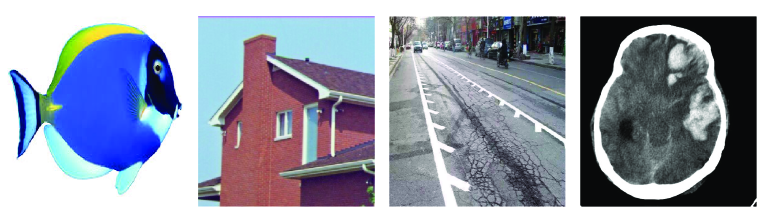
   Figure 2: The original test images : fish, building, lane and liver.

   

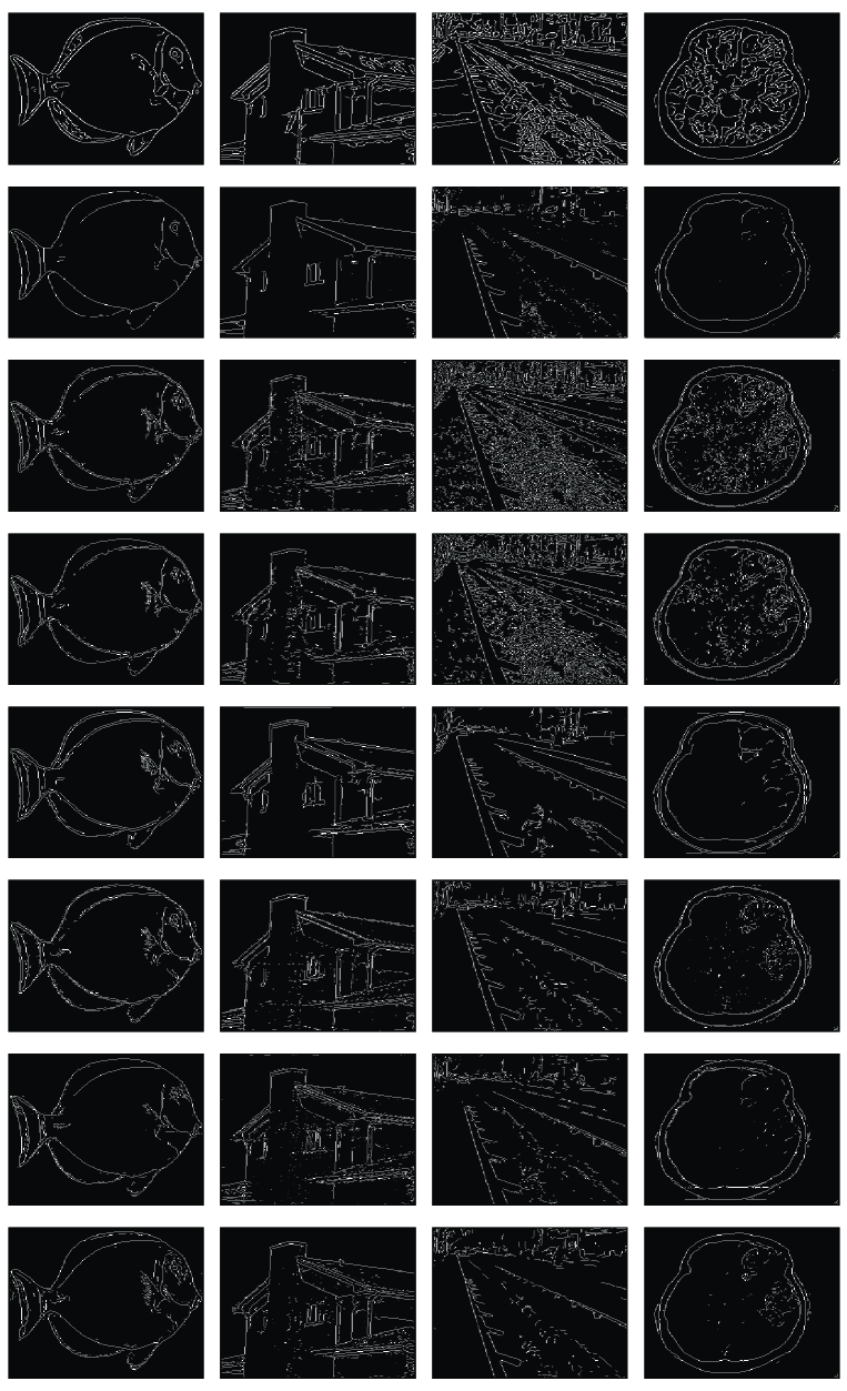
   Figure 3: Comparative Results of Candy, Sobel, DPC, MDPC, QDLA,MQDLA, SDLA, MSDLA approaches, from top to the bottom.

   • Firstly, Fig 3 show us that the phase based approaches DPC, MDPC and our approaches, SDLA, MQDLA, MSDLA can achieve good performance in dealing with details. They can detect a pectoral fin of the fish, shadow region of the building and the white area of the liver. The canny and Sobel did not detect them, because Canny regard them as noise and denoise them. While the Sobel can not find them, because the color contrast between between the shadow region, pectoral fin and their surrounding area is relatively small.

   • Secondly, for the lane, our approaches and Sobel can detect the lane lines very well, while DPC,MDPC and Candy detect too much other information, hence can not figure out the lane lines.

   • Thirdly, the MSDLA has the best performance of all approaches visually.

   Table 1: Scales values $y_{1}$, $y_{2}$ and $s$ for (SDLA,MSDLA,QDLA,MQDLA) and (MDPC, DPC) approaches, respectively.

   Noise	SDLA, MSDLA, QDLA, MQDLA	MDPC, DPC
   Possion noise	$y_{1}=4.5,$ $y_{2}=4.5$	$s=3.5$
   Gaussian noise	$y_{1}=4.5,$ $y_{2}=4.5$	$s=4.5$
   Salt and pepper noise	$y_{1}=5.8,$ $y_{2}=5.8$	$s=6$
   Speckle noise	$y_{1}=4.5,$ $y_{2}=4.5$	$s=5.5$

2. Four different kinds of noise are added to the test images, the scales values of the phased-based approaches (MQDLA, MSDLA, DPC, MDPC) and amplitude-based aproaches (QDLA, SDLA) are showed in Table 1 shows. The SNR denotes the ” signal to noise ratio ”. Figs.5, 6 and 7 show the comparative results. We can have the following conclusion.

   • The MSDLA and SDLA approaches give the better performance than other approaches in detecting edge from the visual comparison. The MSDLA still detect clearly the internal edges of the images corrupted Possion and Gaussian noises, respectively. The Our approaches give the better performance in detecting the noised lane lines than others.

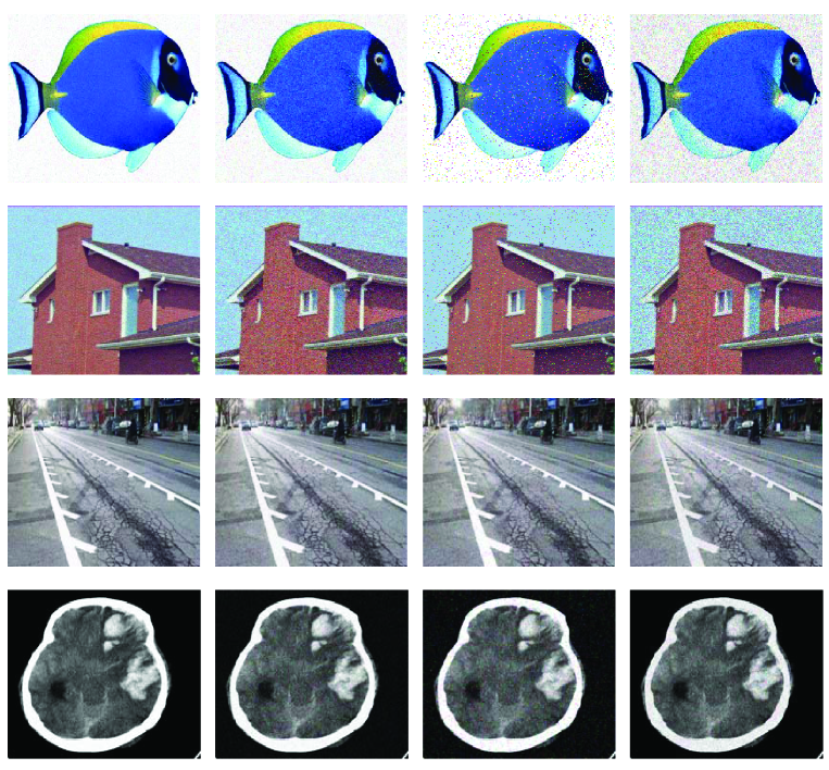
Figure 4: Adding from left to right by Possion, Gaussian, Salt and pepper, Speckle noises on test images.

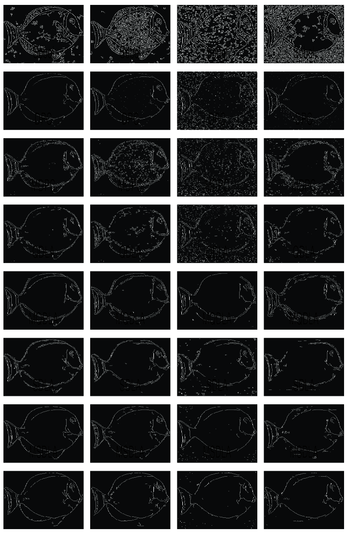
Figure 5: Comparative Results of Candy, Sobel, DPC, MDPC, QDLA,MQDLA, SDLA, MSDLA approaches on fish image from top to the bottom. The first column is added by the Possion, the second is added by the Gaussian, the third column is added by the Salt and pepper, the last column is added by the Speckle noises.

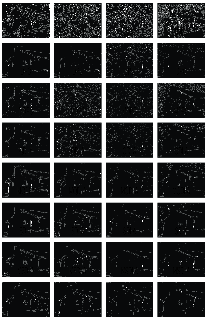
Figure 6: Comparative Results of Candy, Sobel, DPC, MDPC, QDLA,MQDLA, SDLA, MSDLA approaches on building image from top to the bottom. The first column is added by the Possion, the second is added by the Gaussian, the third column is added by the Salt and pepper, the last column is added by the Speckle noises.

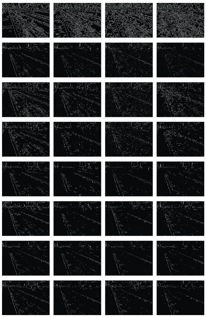
Figure 7: Comparative Results of Candy, Sobel, DPC, MDPC, QDLA,MQDLA,SDLA, MSDLA approaches on lane image from top to the bottom. The first column is added by the Possion, the second is added by the Gaussian, the third column is added by the Salt and pepper, the last column is added by the Speckle noises.

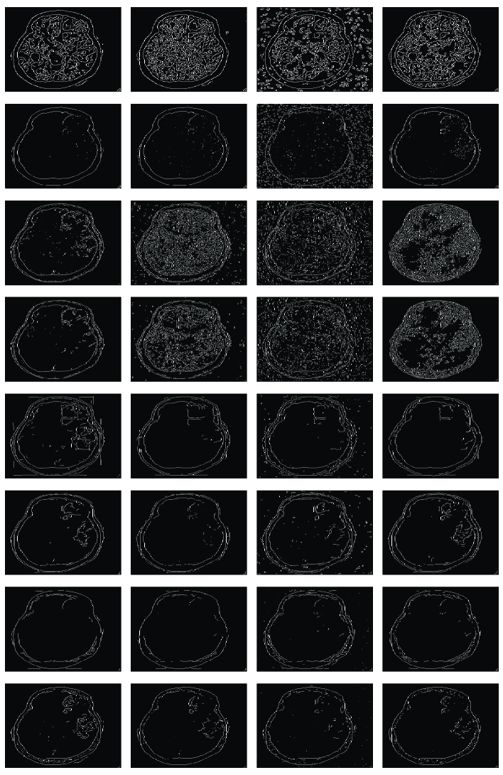
Figure 8: Comparative Results of Candy, Sobel, DPC, MDPC, QDLA,MQDLA, SDLA, MSDLA approaches on liver image from top to the bottom. The first column is added by the Possion, the second is added by the Gaussian, the third column is added by the Salt and pepper, the last column is added by the Speckle noises.

4.2.2 Quantitative analyses

• In this subsection, two well-known objective image quality metrics, namely the peak-signal-to-noise ratio (PSNR) and the structural similarity index measure (SSIM)[33] are analysed. The PSNR is a ratio between maximum power of the signal and the power of corrupting noise. The higher value of PSNR means the better image quality. The SSIM is correlated with the quality perception of the human visual system. The SSIM value is between 0 and 1. 0 means no correlation between images, and 1 means two images are exactly the same.

• The PSNR results of various edge detection approaches of the clear image and different types of noises are shown in tables 2, 4, 6 and 8. The following conclusions are yielded.

  • The MSDLA, Sobel and the SDLA are top three approaches.

  • For the Salt and pepper noise, our proposed approaches MSDLA, SDLA and QDLA outperform than others.

• The SSIM values between the edge detection results of the clear image and different types of noises are shown in tables 3, 5, 7 and 9 show . From the SSIM values in these tables, we have the following conclusions.

  • From table 3, the three top approaches for house image are the MSDLA, the QDLA, the Sobel.

  • From table 5, the three top approaches for fish image are the MSDLA, the SDLA, the Sobel.

  • Form table 7, the three top approaches for lane image are the MSDLA, the MQDLA and the QDLA for Gaussian, Salt and pepper, and Speckle noises. For Possion noise, the top three approaches are Sobel , the MSDLA and the MQDLA.

  • Form table 9, the three top approaches for liver image are the SDLA, the QDLA, the Sobel.

  • For the Salt and pepper noise, Our proposed approaches MSDLA, SDLA, QDLA outperform than others.

Table 2: PSNR comparison values for the building image corrupted by different types of noises.

Building Image	Possion noise	Gaussian noise	Salt and pepper noise	Speckle noise
SNR	21.9366	15.1953	15.1704	12.1711
QDLA	12.8536	12.4640	12.1802	12.0699
MQDLA	12.3692	11.9885	11.8352	11.6404
SDLA	13.8576	13.2010	12.7853	13.4110
MSDLA	22.2653	13.4446	18.6807	13.0943
DPC	11.3587	8.7472	8.4344	8.9117
MDPC	12.2731	10.5810	9.0634	10.6015
Sobel	17.8588	15.3887	11.2699	14.2133
Canny	10.4607	7.6753	7.7588	7.2481

Table 3: SSIM comparison values for the building image corrupted by different types of noises.

Building Image	Possion noise	Gaussian noise	Salt and pepper noise	Speckle noise
SNR	21.0366	15.1953	15.1704	13.1711
QDLA	0.7022	0.6383	0.5699	0.5573
MQDLA	0.6052	0.5512	0.4785	0.4803
SDLA	0.7154	0.6952	0.5591	0.6212
MSDLA	0.9299	0.6957	0.7240	0.6557
DPC	0.4412	0.1357	0.0778	0.1997
MDPC	0.5505	0.3541	0.1036	0.3495
Canny	0.5133	0.2679	0.2594	0.2645
Sobel	0.8831	0.7297	0.2528	0.5842

Table 4: PSNR comparison values for the fish image corrupted by different types of noises.

Fish Image	Possion noise	Gaussian noise	Salt and pepper noise	Speckle noise
SNR	25.0937	18.8141	18.8221	17.7628
QDLA	14.5343	13.2038	13.0903	12.4840
MQDLA	13.5543	13.0246	12.0444	13.2878
SDLA	16.3664	15.1091	14.6779	14.6604
MSDLA	15.7743	14.5419	14.2802	14.6199
DPC	13.6042	10.9823	10.3732	11.4006
MDPC	14.2133	12.5110	11.1096	12.6723
Sobel	21.1900	18.0154	11.5467	16.5963
Canny	12.1900	8.7313	8.8579	7.3773

Table 5: SSIM comparison values for the fish image corrupted by different types of noises.

Fish Image	Possion noise	Gaussian noise	Salt and pepper noise	Speckle noise
SNR	25.0937	18.8141	18.8221	17.7628
QDLA	0.8035	0.7365	0.7107	0.6848
MQDLA	0.7522	0.7132	0.6001	0.7125
SDLA	0.8238	0.8001	0.7009	0.7665
MSDLA	0.8131	0.7569	0.7038	0.7529
DPC	0.7396	0.4992	0.1867	0.5401
MDPC	0.7749	0.6554	0.2915	0.6604
Canny	0.6342	0.4562	0.3292	0.3106
Sobel	0.9320	0.8285	0.3157	0.7463

Table 6: PSNR comparison values for the lane image corrupted by different types of noises.

Lane Image	Possion noise	Gaussian noise	Salt and pepper noise	Speckle noise
SNR	22.0935	15.2766	13.6430	22.0774
QDLA	14.3320	13.2512	13.6430	12.9391
MQDLA	14.9426	13.6255	13.0074	12.9169
SDLA	15.6826	14.2150	13.9144	14.1387
MSDLA	15.6777	14.5740	13.6209	13.7620
DPC	8.0192	7.6057	7.2626	7.2760
MDPC	8.5859	8.2340	7.8697	8.0899
Sobel	17.7746	14.7715	12.1496	13.9127
Canny	11.6715	8.3611	7.6715	7.3495

Table 7: SSIM comparison values for the lane image corrupted by different types of noises.

Lane Image	Possion noise	Gaussian noise	Salt and pepper noise	Speckle noise
SNR	22.0935	15.2766	13.6430	22.0774
QDLA	0.7217	0.6685	0.6295	0.6294
MQDLA	0.7618	0.6489	0.6100	0.5989
SDLA	0.7329	0.6424	0.6069	0.6466
MSDLA	0.7743	0.6919	0.6529	0.6437
DPC	0.2441	0.1472	0.0811	0.1301
MDPC	0.2871	0.1882	0.1195	0.1859
Canny	0.7118	0.4349	0.3675	0.3387
Sobel	0.8062	0.6236	0.3300	0.5377

Table 8: PSNR comparison values for the liver image corrupted by different types of noises.

Liver Image	Possion noise	Gaussian noise	Salt and pepper noise	Speckle noise
SNR	23.1723	14.2158	9.9592	14.3338
QDLA	13.8431	14.6314	13.1914	14.3338
MQDLA	13.9111	13.9586	12.4828	12.8169
SDLA	15.9428	15.8476	14.2909	14.7327
MSDLA	15.5237	16.0723	15.1567	15.3658
DPC	11.5193	8.1548	8.7022	8.4423
MDPC	12.6735	9.2078	9.1819	9.1214
Sobel	23.3218	19.4960	12.3385	17.7509
Canny	12.7378	9.8212	8.6939	9.9151

Table 9: SSIM comparison values for the liver image corrupted by different types of noises.

Liver Image	Possion noise	Gaussian noise	Salt and pepper noise	Speckle noise
SNR	23.1723	14.2158	9.9592	14.3338
QDLA	0.7253	0.7921	0.6924	0.7936
MQDLA	0.7207	0.6958	0.6820	0.6661
SDLA	0.8161	0.8026	0.7456	0.7863
MSDLA	0.8073	0.8075	0.7439	0.7787
DPC	0.5531	0.2835	0.2178	0.4564
MDPC	0.6307	0.4184	0.2814	0.4913
Canny	0.7760	0.6437	0.3858	0.6142
Sobel	0.9465	0.8695	0.3638	0.8350

5 Conclusion and Future Work

In this paper, firstly, by using the generalized Cauchy$-$Riemann equations, we not only obtain the relations between the local features of quaternion Hardy function in higher dimensional spaces in Corollary 3.1, but also in Theorem 3.1 gives the more detail relations between the four components of $f$ and its local attenuation in higher dimensional spaces. Secondly, there are different types of edge detection filters, which are connected between components of the quaternion Hardy function and its local features. Finally, the comparison examples have numerically confirmed that our proposed approaches perform better than the conventional ones. on one hand, our proposed approaches can not only detect the whole smooth region, but also the local small change region. On the other hand, our approaches have a good performance in denoising various types of the noised images.

In the future, Kou [23] defined the generalized quaternion analytic signal in invoking the quaternion linear canonical transform, which has six parameters, when these parameters chosen the special values, the quaternion linear canonical transform reduces to quaternion Fourier transform, and Kou [23] applied the generalized quaternion analytic signal to do envelope of the image, which inspires us to develop more image processing applications by using the generalized quaternion analytic signal.

Acknowledgments

Kit Ian Kou acknowledges financial support by The Science and Technology Development Fund, Macau SAR (File no. FDCT/085/2018/A2).Xiaoxiao Hu acknowledges financial support from the Research Development Foundation of Wenzhou Medical University (QTJ18012)

References

- [1] Q. Li, P.L. Shui, Noise-robust color edge detection using anisotropic morphological directional derivative matrix ,Signal Processing,165(2019), pp. 90–103.
- [2] L.-C Wang, S.-Q. Geng, B.-Y. Liu, Y. Jin, Ballistocardiogram heart rate detection: Improved methodology based on a three-layer filter , Measurement, 19(2020), DOI: 10.1016/j.measurement.2019.106956.
- [3] Y. Li, S. Wang, Q Tian and X.-Q.Ding, A survey of recent advances in visual feature detection , Neurocomputing, (149)2015, pp. 736–751.
- [4] E. Gengel, A. Pikovsky, Phase demodulation with iterative Hilbert transform embeddings, Signal Processing, 165(2019), pp. 115–129.
- [5] A. Venkitaraman, S. Chatterjee and p. Handel, On Hilbert transform, analytic signal, and modulation analysis for signals over graphs , Signal Processing, 156(2019), pp. 106–115.
- [6] S. Bernstein, J.-L. Bouchot, M. Reinhardt and B. Heise, Generalized analytic signals in image processing: Comparison, theory and applications, in Quaternion and Clifford Fourier Transforms and Wavelets, Springer, 2013, pp. 221–246.
- [7] T. Bulow and G. Sommer, Hypercomplex signals-a novel extension of the analytic signal to the multidimensional case, IEEE Transactions on Signal Processing, 49 (2001), pp. 2844–2852.
- [8] T. A. Ell, N. Le Bihan and S. J. Sangwine, Quaternion Fourier transforms for signal and image processing, John Wiley & Sons, 2014.
- [9] M. Felsberg and G. Sommer, The monogenic signal, IEEE Transactions on Signal Processing, 49 (2001), pp. 3136–3144.
- [10] C. Zou, K. I. Kou and Y. Wang, Quaternion Collaborative and Sparse Representation With Application to Color Face Recognition, IEEE Transactions on Image Processing, 25(7)(2016), pp. 3287-3302.
- [11] Y. H. Xia and K. I. Kou, Linear Quaternion Differential Equations: Basic Theory and Fundamental Results, Studies in Applied Mathematics, 141(1)(2018), pp. 3-45.
- [12] C. Safarian and T. Ogunfunmi, The quaternion minimum error entropy algorithm with fiducial point for nonlinear adaptive systems, Signal Processing, 163 (2019), pp. 188–200.
- [13] L.H. Jin, Z.L. Zhu, E.M. Song and X.Y. Xu, An effective vector filter for impulse noise reduction based on adaptive quaternion color distance mechanism , Signal Processing, 155 (2019), pp. 334–345.
- [14] Y. Liu, Y. Zheng, J. Lu, J. Cao and L. Rutkowski, Constrained quaternion-variable convex optimization: a quaternion-valued recurrent neural network approach, IEEE Transactions on Neural Networks and Learning Systems, DOI: 10.1109/TNNLS.2019.2916597, 2019.
- [15] Y. Liu, D. Zhang, J. Lou, J. Lu and J. Cao, Stability analysis of quaternion-valued neural networks: Decomposition and direct approaches, IEEE Transactions on Neural Networks and Learning Systems, 29(9)(2018), pp. 4201-4211.
- [16] M. Felsberg and G. Sommer, The monogenic scale-space: A unifying approach to phase-based image processing in scale-space, Journal of Mathematical Imaging and vision, 21 (2004), pp. 5–26.
- [17] S. L. Hahn, Multidimensional complex signals with single-orthant spectra, Proceedings of the IEEE, 80 (1992), pp. 1287–1300.
- [18] S. L. Hahn, Hilbert Transforms in Signal Processing, Artech House, Norwood, MD, 1996.
- [19] S. L. Hahn and K. M. Snopek, Wigner distributions and ambiguity functions of 2-d quaternionic and monogenic signals, IEEE Transactions on Signal Processing, 53 (2005), pp. 3111–3128.
- [20] X. Hu and K. I. Kou, Phase-based edge detection algorithms. Mathematical Methods in the Applied Sciences, 2017, pp. 1-20.
- [21] X. Hu and K. I. Kou, Quaternion fourier and linear canonical inversion theorems, Mathematical Methods in the Applied Sciences, 40 (2017), pp. 2421-2440.
- [22] R. Jain, R. Kasturi, and B. G. Schunck, Machine vision, vol. 5, McGraw-Hill New York, 1995.
- [23] K. I. Kou, M.-S. Liu, J. P. Morais and C. Zou, Envelope detection using generalized analytic signal in 2d qlct domains, Multidimensional Systems and Signal Processing, (2016), pp. 1–24.
- [24] K.-I. Kou and T. Qian, The paley–wiener theorem in rn with the clifford analysis setting, Journal of Functional Analysis, 189 (2002), pp. 227–241.
- [25] P. Kovesi, Image features from phase congruency, Videre: Journal of computer vision research, 1 (1999), pp. 1–26.
- [26] E. M Stein and W. Guido, Introduction to fourier analysis on Euclidean spaces, Princeton University Press, 1990.
- [27] M. Sonka, V. Hlavac and R. Boyle, Image processing, analysis, and machine vision, Cengage Learning, 2014.
- [28] Y. Yang, K. I. Kou and C. Zou, Edge detection methods based on modified differential phase congruency of monogenic signal, Multidimensional Systems and Signal Processing, (2017), pp. 1–21.
- [29] Y. Yang, T. Qian and F. Sommen, Phase derivative of monogenic signals in higher dimensional spaces, Complex Analysis and Operator Theory, 6 (2012), pp. 987–1010.
- [30] B. Zitova and J. Flusser, Image registration methods: a survey, Image and Vision Computing, 21 (2003), pp. 977–1000.
- [31] C. Zuppinger, Edge-detection for contractility measurements with cardiac spheroids, Stem Cell-Derived Models in Toxicology, (2017), pp. 211–227.
- [32] A. Hore and D. Ziou, Image quality metrics: PSNR vs. SSIM , IEEE In Pattern Recognition (ICPR), 20th International Conference on 2010 Aug 23, pp. 2366-2369 (2010).
- [33] Z. Wang, A. C. Bovik, H. R. Sheikh and E. P.Simoncelli, Image quality assessment: from error visibility to structural similarity, IEEE Transactions on Image Processing, 13(4)(2004),pp. 600-612.